Identifying Influential and Vulnerable Nodes in Interaction Networks through Estimation of Transfer Entropy Between Univariate and Multivariate Time Series

Abstract

Transfer entropy (TE) is a powerful tool for measuring causal relationships within interaction networks. Traditionally, TE and its conditional variants are applied pairwise between dynamic variables to infer these causal relationships. However, identifying the most influential or vulnerable node in a system requires measuring the causal influence of each component on the entire system and vice versa. In this paper, I propose using outgoing and incoming transfer entropy—where outgoing TE quantifies the influence of a node on the rest of the system, and incoming TE measures the influence of the rest of the system on the node. The node with the highest outgoing TE is identified as the most influential, or “hub”, while the node with the highest incoming TE is the most vulnerable, or “anti-hub”. Since these measures involve transfer entropy between univariate and multivariate time series, naive estimation methods can result in significant errors, particularly when the number of variables is comparable to or exceeds the number of samples. To address this, I introduce a novel estimation scheme that computes outgoing and incoming TE only between significantly interacting partners. The feasibility of this approach is demonstrated by using synthetic data, and by applying it to a real data of oral microbiota. The method successfully identifies the bacterial species known to be key players in the bacterial community, demonstrating the power of the new method.

I Introduction

Causal inference in interacting dynamic systems is a critical area of study that aims to understand the cause-and-effect relationships within complex systems [1, 2, 3, 4, 5, 6, 7, 8, 9, 10, 11, 12, 13, 14, 15, 16]. These systems can be found in various fields, including neuroscience, economics, and ecology. The goal is to distinguish true causal interactions from mere correlations, which is essential for predicting system behavior and designing effective interventions

Information theory offers rigorous foundation for causal inference by quantifying the information shared between a pair of variables $X$ and $Y$ through mutual information $I(X,Y)$ defined as:

$$I(X,Y)\equiv\left\langle\log_{2}\left(\frac{P(X,Y)}{P(X)P(Y)}\right)\right\rangle$$ (1)

where $P(X)$ and $P(Y)$ are the marginal probability distributions for the random variables $X$ and $Y$, $P(X,Y)$ are their joint probability distribution, and $\langle\rangle$ denote the expectation value. In systems with more than two variables, one often seeks the direct correlation between $X$ and $Y$ after accounting for other variables. Denoting all variables other than $X$ and $Y$ by $Z$, the conditional mutual information $I(X,Y/Z)$ is defined as:

$$I(X,Y/Z)\equiv\left\langle\log_{2}\left(\frac{P(X,Y/Z)}{P(X/Z)P(Y/Z)}\right)\right\rangle,$$ (2)

which quantifies the direct correlation between $X$ and $Y$.

In dynamic systems, given two time series $X(t)$ and $Y(t)$, where the integer $t$ is an index for a discretized time, one might initially attempt to quantity the causal influence of $X$ on $Y$ using $I(X_{-},Y(t))$, where $X_{-}\equiv(X(1),X(2),\cdots X(t-1))$ represents the past history of $X$. However, as previously mentioned, $I(X_{-},Y(t))$ only quantifies the shared information between the history of $X$ and the present state of $Y$, not the causal influence of $X$ on $Y$. It is possible that $Y$ actually causes $X$, which could still result in a non-zero value of $I(X_{-},Y(t))$. Therefore, to quantify the true causal influence of $X$ on $Y$, we must correct for the effect due to the history of $Y$, using the measure:

$$T_{X\to Y}={I}(X_{-},Y(t)/Y_{-}).$$ (3)

This is known as transfer entropy (TE) from $X$ to $Y$ [1]. Transfer entropy can also be expressed as:

$$T_{X\to Y}=H(Y(t)/Y_{-})-H(Y(t)/X_{-},Y_{-}),$$ (4)

where

$$H(Y(t)/Y_{-}) \equiv \langle-\log_{2}P(Y(t)/Y_{-})\rangle$$

$$H(Y(t)/X_{-},Y_{-}) \equiv -\langle\log_{2}P(Y(t)/X_{-},Y_{-})\rangle.$$ (5)

Here, the conditional entropies $H(Y(t)/Y_{-})$ and $H(Y(t)/X_{-},Y_{-})$ represent the uncertainties of $Y(t)$ after observing the history of $Y$ and after observing the histories of both $X$ and $Y$, respectively. Thus, $T_{X\to Y}$ can be interpreted as the reduction in the uncertainty of $Y(t)$ after observing the history of $X$, given that we already know the history of $Y$. It can be proved that $T_{X\to Y}$ as well as $H(Y(t)/Y_{-})$ and $H(Y(t)/X_{-},Y_{-})$ are all non-negative (see Appendex A). Specifically, this implies that if $Y(t)$ is completely determined by $Y_{-}$ such that $H(Y(t)/Y_{-})=0$, then $T_{X\to Y}=0$. The intuitive interpretation is clear: If there is no uncertainty on $Y(t)$ after we observe $Y_{-}$, then obviously there is no additional uncertainty to be removed by knowing $X_{-}$.

In systems with more than two time series, we are often interested in the direct causal influence of $X$ on $Y$ after accounting for indirect effects due to other variables. Denoting the multivariate time series of variables other than $X$ and $Y$ by $Z$, the direct causal influence of $X$ on $Y$ is quantified by: quantity [9, 10, 11, 12]

$$T_{(X\to Y)/Z}\equiv I(X_{-},Y(t)/Y_{-},Z_{-}).$$ (6)

This measure is called multivariate transfer entropy, conditional transfer entropy, causation entropy, or full conditional mutual information [9, 10, 11, 12, 13, 14, 15, 16].

Although there are nuances in interpreting transfer entropy and its conditional variant as information flow or causal influence quantification [17], these measures have been widely used to uncover causal relationships in complex networks, including neural networks [18, 19, 20], social networks [21], and gene regulatory networks [22, 23].

However, in all these applications, the causal relationship between each pair of variables in the network was estimated. In this work, I focus on finding the most influential components in the network, the hubs, and most vulnerable component, which I will refer to as “anti-hub”. Identifying hubs and anti-hubs is crucial for understanding, managing, and optimizing complex systems across various domains, from biology and ecology to engineering and social sciences. To find such influential or vulnerable components, we must quantify the causal relation of each node to the rest of the system and vice versa. I refer to these measures as “outgoing TE (OutTE)” and “incoming TE (InTE)”, respectively. Here, we only have two variables in the system so that we can use Eq.(3), but with the source variable being univariate and the target variable being multivariate, or vice versa. As will be elaborated further, naive estimates of such quantities can lead to significant estimation errors, particularly when the number of variables is comparable to or larger than the length of the time series. In this work, I will introduce the novel estimation method for the OutTE and InTE, where estimation is performed only between significantly interacting partners.

The outline of the paper is as follows. In section II, I will illustrate the estimation problem of outTE and inTE using synthetic data from simple models, showing how estimation error increases as the number of unrelated nodes increases. In section III, I will introduce the novel estimation method for the OutTE and InTE, which overcomes the estimation problem. In section IV, I will apply my method to microbiota data, showing that the new estimation method successfully identifies the bacterial species known to be key players in the bacterial community. The section V concludes the paper.

II Estimation problem of Outgoing and Incoming Transfer entropies.

The focus of this work is on identifying hub and anti-hub nodes in an interaction network–nodes that exert significant influences on the rest of the system, and the those that are most influenced by the rest of the system, respectively. To identify hub nodes, we need to compute OutTE for each node $X$, ${\rm OutTE}(X)\equiv T_{X\to{\rm rest}}$, where “rest” denotes the collection of all nodes except $X$. We then select the nodes with the largest values of ${\rm OutTE}$. Similarly, anti-hubs are identified by computing ${\rm InTE}(X)\equiv T_{{\rm rest}\to X}$ and selecting the nodes with the largest values of ${\rm InTE}$. However, in practice, the true values of these quantities are not available and must be estimated from data, which can introduce estimation errors.

For example, consider microbiota data obtained from the saliva of a subject observed for a year [24], which will be discussed further in a later section. There are 879 nodes, where each node represents an operational taxonomic unit (OTU) in the microbiota, and the time-series length is 226 days. Transfer entropy from each of the node to the remaining 878 nodes can be estimated using a publically available tool [25], and the result of such an estimate is zero for all of the 879 nodes! This suggests that the estimate $\widehat{\rm OutTE}(X)$ is much smaller than the true value ${\rm OutTE}(X)$, where $\hat{\theta}$ denotes the estimate of a measure $\theta$ obtained from the data. In fact, the conditional entropies $H(Y(t)/Y_{-})$ and $H(Y(t)/(X_{-},Y_{-})$ in Eq.(5) tend to underestimate the true values when the sample size is small, due to insufficient observation of events (Appendix B). From the fact that $\hat{H}(Y(t)/Y_{-})\geq\widehat{H}(Y(t)/X_{-},Y_{-})$ (Appendix A), we see that if the underestimation is so severe that $\hat{H}(Y(t)/Y_{-})\simeq 0$, then $H(Y(t)/X_{-},Y_{-})\simeq 0$, leading to $\hat{T}_{X\to Y}=\hat{H}(Y(t)/Y_{-})-\hat{H}(Y(t)/X_{-},Y_{-})\simeq 0$.

To illustrate this problem, consider a simple system consisting of a sender S and a recipient R, as shown in Fig. 1. The state of each node, denoted as $S(t)$ and $R(t)$, is either $0$ or $1$. $S(t)$ is completely random, chosen between 0 and 1 with equal probability. $R(0)$ is also random, but $R(t)$ for $t>0$ is completely determined by $S(t-1)$ and $R(t-1)$ according to the rule $R(t)=S(t-1)\oplus R(t-1)$. In the absence of the knowledge of the sender’s state, the dynamics of the recipient node is completely random, leading to $H(R(t)/R_{-})=1$ bit. Additionally, since $R(t)$ is entirely determined by $S(t-1)$ and $R(t-1)$, $H(R(t)/R_{-},S_{-})=0$, leading to $T_{S\to R}=1$ bit. In contrast, ${T}_{R\to S}$ is zero bits, as $H(S(t)/S_{-})=H(S(t)/R_{-},S_{-})=0$, resulting in $T_{R\to S}=0$. Note that the dynamics here is Markovian since the entire dynamics depends only on the previous states of S and R.

Now, consider the estimates of the information-theoretic measures from data. Suppose we have four observations of state transitions $(S,R)$:

$$(0,0) \to (0,0),\quad(0,1)\to(1,1),\quad(1,0)\to(1,1),\quad(1,1)\to(1,0).$$ (7)

In this case, the empirical conditional probability distribution $\hat{P}(R(t)/S_{-},R_{-})$ happens to coincide with the true conditional probability distribution $P(R(t)/S_{-},R_{-})$, so the estimated transfer entropy equals the true value. Therefore, $\hat{T}_{S\to R}=1$ bit and ${\hat{T}}_{R\to S}=0$ bits.

Now, suppose other nodes labeled ${\rm C}_{1},{\rm C}_{2},\cdots{\rm C}_{n}$ take random values of $0$ or $1$ and are entirely disconnected from the rest of the system. I will call these “confounding nodes” (see Fig. 1). The true values of OutTE(S) and OutTE(R) remain unaffected, as the dynamics of ${\rm C}_{1},{\rm C}_{2},\cdots{\rm C}_{n}$ are independent of S and R. However, they can severely affect the estimated values. Let us assume just one confounding node C is added to the example in Eq.(7) so that the four observation for the transitions of the states $(S,R,C)$ become:

$$(0,0,1) \to (0,0,1),\quad(0,1,0)\to(1,1,1),\quad(1,0,0)\to(1,1,0),\quad(1,1,1)\to(1,0,0)$$ (8)

Now the dynamics of $(R,C)$ estimated by the data above is completely deterministic. That is, the only four observed transitions for $(R,C)$ are

$$(0,1) \to (0,1),\quad(1,0)\to(1,1),\quad(0,0)\to(1,0),\quad(1,1)\to(0,0),$$ (9)

which are all unique. This leads to $\hat{H}(R(t),C(t))/R_{-},C_{-})=\hat{H}(R(t),C(t))/R_{-},C_{-},S_{-})=0$, resulting in $\widehat{\rm OutTE}(S)=\hat{T}_{S\to(R,C)}=0$, which represents a drastic underestimation compared to the true value of ${\rm OutTE}(S)=1$. This artifact arises when the number of variables is comparable to or larger than the number of samples. In such situations, most observed transitions become rare events, typically appearing only once in the data, leading to the underestimation of the values of conditional entropy (Appendix B).

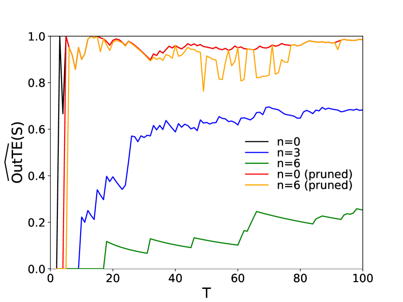
Figure 2: $\widehat{\rm OutTE}(S)$ in the SR model as a function of $T$, for $n=0,3,6$ without pruning (black, blue, and green lines, respectively), and with pruning (red and orange lines for $n=0$ and $6$, respectively).

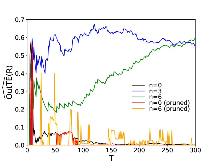
Figure 3: $\widehat{\rm OutTE}(R)$ in the SR model as a function of $T$, for $n=0,3,6$ without pruning (black, blue, and green lines, respectively), and with pruning (red and orange lines for $n=0$ and $6$, respectively).

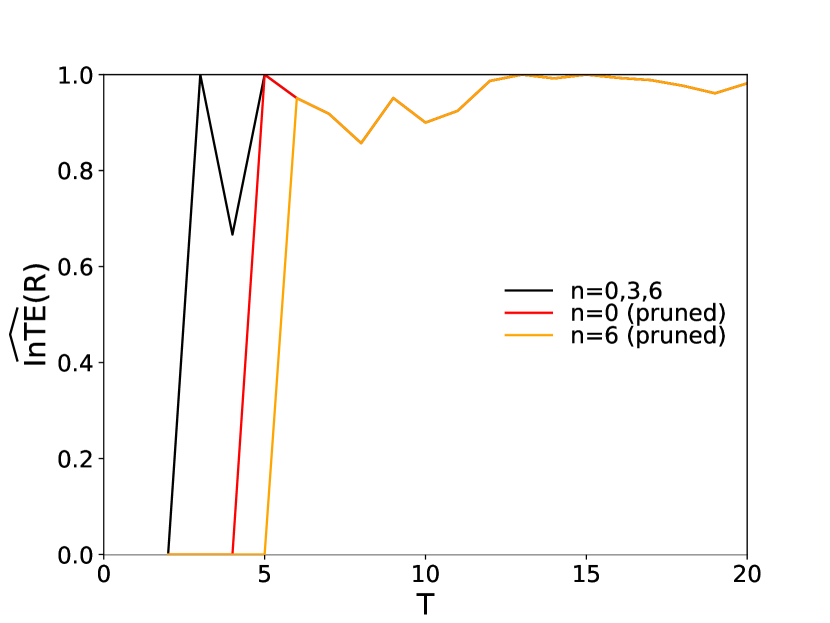
Figure 5: $\widehat{\rm InTE}(R)$ in the SR model as a function of $T$, for $n=0,3,6$ without pruning (black line), and with pruning (red and orange lines for $n=0$ and $6$, respectively).

A synthetic time series of length 300 were generated using the probability distribution of the model in Fig 1, referred to as the SR model. The estimated values $\widehat{\rm OutTE}$ and $\widehat{\rm InTE}$ were computed from the empirical distribution when partial series up to length $T$ was used. I assumed Markovian dynamics from the start, so the number of observed transition is $T-1$. Computations were performed using the JIDT toolkit [25]. The graphs of $\widehat{\rm OutTE}(S)$, $\widehat{\rm OutTE}(R)$, $\widehat{\rm InTE}(S)$ and $\widehat{\rm InTE}(R)$ are shown in Figs. 2, 3, 4, and 5, respectively, for the number of confounding nodes $n=0$ (black line) , $3$ (blue line), and $6$ (green line). We observe that $\widehat{\rm OutTE}(S)$ is smaller than the true value of ${\rm OutTE}(S)=1$ bit for small sample sizes, but begins to converge to the true value around $T\simeq 10$ for $n=0$. As the confounding nodes are added, the underestimation becomes more severe for a given $T$, and convergence becomes slower. In the case of ${\rm OutTE}(R)$, whose true value is zero, we now face an overestimation problem in the presence of confounding nodes (Fig. 3), because although both $\hat{H}(S(t),C_{1}(t),\cdots,C_{n}(t)/S(t-1),C(t-1),\cdots,C_{n}(t-1))$ and $\hat{H}(S(t),C_{1}(t),\cdots,C_{n}(t)/R(t-1),S(t-1),C(t-1),\cdots,C_{n}(t-1))$ decrease as $T$ increases, the latter term decreases faster. However, since $\hat{H}(S(t),C_{1}(t),\cdots,C_{n}(t))/(S(t-1),C_{1}(t-1),\cdots,C_{n}(t-1))\geq\hat{H}(S(t),C_{1}(t),\cdots,C_{n}(t))/(R(t-1),S(t-1),C_{1}(t-1),\cdots,C_{n}(t-1))\geq 0$, we expect that $\lim_{T\to\infty}\widehat{\rm OutTE}(R)=0$ for a given $n$. In the case of ${\rm InTE}(S)$, whose true value is zero, we again encounter an overestimation problem as the confounding nodes are added (Fig. 4). Finally, the estimate of ${\rm InTE}(R)$, whose true value is one bit, remains unaffected by the presence of the confounding nodes, as shown by the black line in Fig. 5. Note that the first term in Eq. (4), $H(R(t)/R_{-})$, does not depend on the confounding nodes, nor does its estimate $\hat{H}(R(t)/R_{-})$. The only possible dependence on the confounding nodes originates from the estimate $\hat{H}(R(t)/R_{-},S_{-},{C_{1}}_{-},\cdots,{C_{N}}_{-})$. However, the values of $R(t-1)$ and $S(t-1)$ uniquely determine the value of $R(t)$ in this model, and the addition of confounding nodes does not change this determinism. Therefore, $\hat{H}(R(t)/R_{-},S_{-},{C_{1}}_{-},\cdots,{C_{N}}_{-})=0$ regardless of the number of confounding nodes, leading to ${\rm InTE}(R)\equiv T_{(S,C_{1},\cdots,C_{N})\to R}=\hat{H}(R(t)/R_{-})$, which is independent of the confounding nodes.

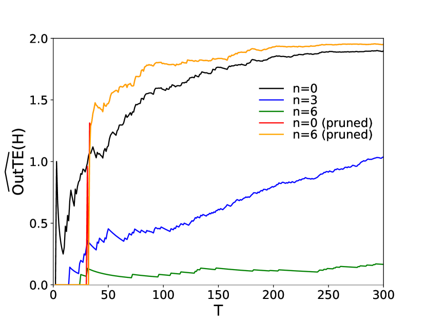
Figure 7: $\widehat{\rm OutTE}(H)$ in the HSAR model as a function of $T$, for $n=0,3,6$ without pruning (black, blue, and green lines, respectively) and with pruning (red and orange lines for $n=0$ and $6$, respectively).

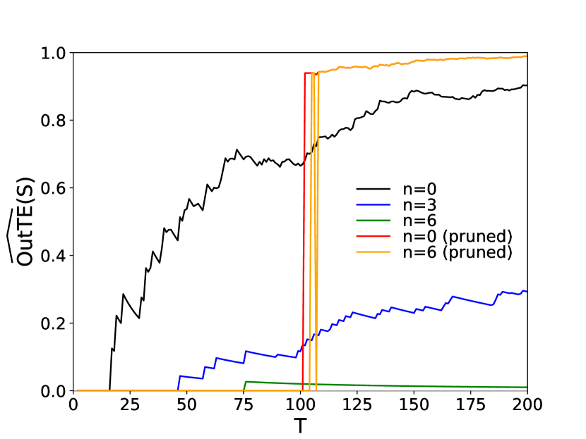
Figure 8: $\widehat{\rm OutTE}(S)$ in the HSAR model as a function of $T$, for $n=0,3,6$ without pruning (black, blue, and green lines, respectively), and with pruning (red and orange lines for $n=0$ and $6$, respectively).

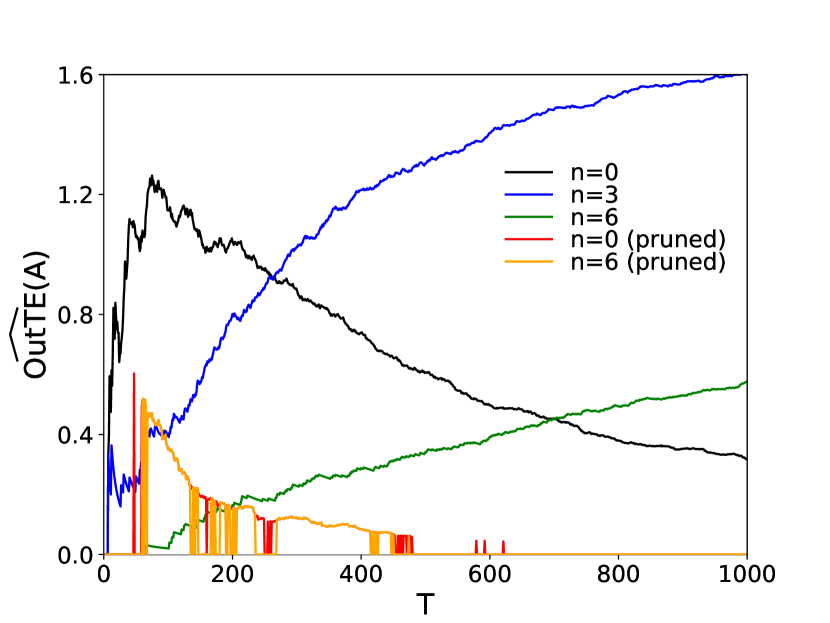
Figure 9: $\widehat{\rm OutTE}(A)$ in the HSAR model as a function of $T$, for $n=0,3,6$ without pruning (black, blue, and green lines, respectively), and with pruning (red and orange lines for $n=0$ and $6$, respectively).

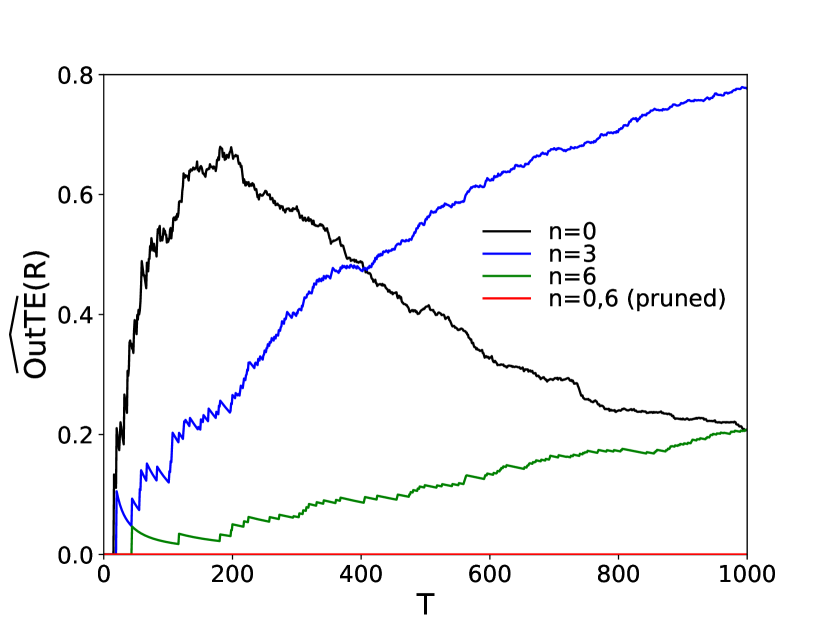
Figure 10: $\widehat{\rm OutTE}(R)$ in the HSAR model as a function of $T$, for $n=0,3,6$ without pruning (black, blue, and green lines, respectively), and with pruning (red and orange lines for $n=0$ and $6$, respectively).

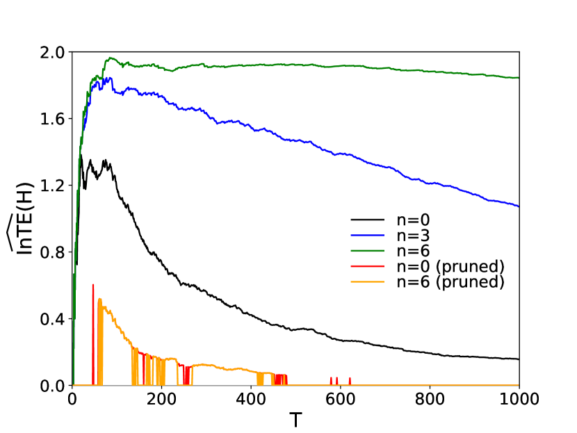
Figure 11: $\widehat{\rm InTE}(H)$ in the HSAR model as a function of $T$, for $n=0,3,6$ without pruning (black, blue, and green lines, respectively), and with pruning (red and orange lines for $n=0$ and $6$, respectively).

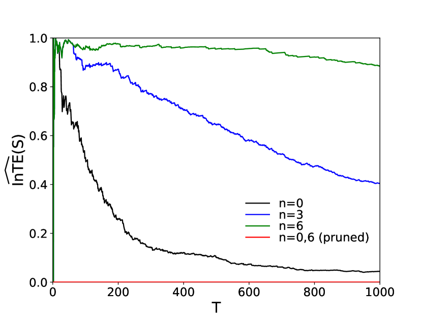
Figure 12: $\widehat{\rm InTE}(S)$ in the HSAR model as a function of $T$, for $n=0,3,6$ without pruning (black, blue, and green lines, respectively), and with pruning (red and orange lines for $n=0$ and $6$, respectively).

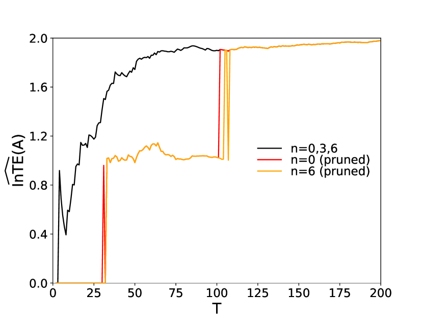
Figure 13: $\widehat{\rm InTE}(A)$ in the HSAR model as a function of $T$, for $n=0,3,6$ without pruning (black lines), and with pruning (red and orange lines for $n=0$ and $6$, respectively).

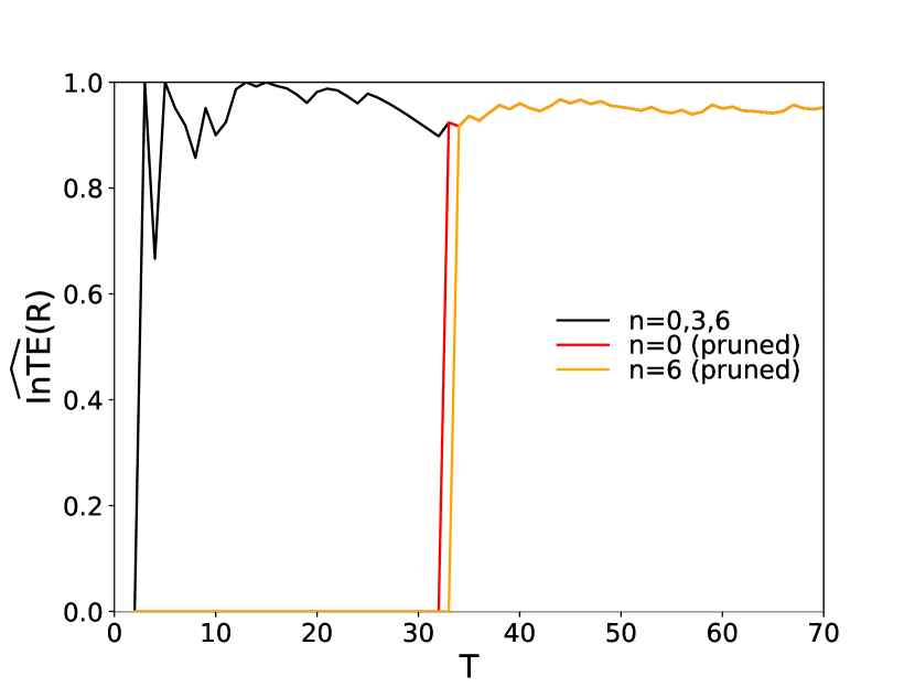
Figure 14: $\widehat{\rm InTE}(R)$ in the HSAR model as a function of $T$, for $n=0,3,6$ without pruning (black lines), and with pruning (red and orange lines for $n=0$ and $6$, respectively).

I conducted a similar analysis on a system containing a hub H, a sender node S, an anti-hub A, and a receiver node R, shown in Fig. 6, which I will call HSAR model. Here the hub node sends two independent bits of information to two nodes A and R, and S sends one bit of information to A, so that A receives one bit of information from H and another from S, and R receives ont bit of information from H. The estimates $\widehat{\rm OutTE}(H)$, $\widehat{\rm OutTE}(S)$, $\widehat{\rm OutTE}(A)$, $\widehat{\rm OutTE}(R)$, $\widehat{\rm InTE}(H)$, $\widehat{\rm InTE}(S)$, $\widehat{\rm InTE}(A)$, and $\widehat{\rm InTE}(R)$, are shown in Figs.7, 8, 9, 10, 11, 12, 13, and 14 for the number $n$ of confounding nodes $n=0,3,6$, with black, blue, and green lines, respectively. The results are qualitatively similar to those of the previous model with the sender and the receiver.

III The Method for accurate estimation of Outgoing and Incoming transfer entropy

In the previous examples, the estimation errors were due to the proliferation of variables caused by confounding nodes. If we had eliminated unrelated nodes beforehand, the estimation error would have been reduced. Therefore, instead of estimating estimating OutTE from a node to all other nodes, and InTE to the node from all others, we first take a pruning step where only nodes causally related the node of interest are selected. That is, we construct a directed binary network where an edge $X\to Y$ exists if and only if $\widehat{T}_{(X\to Y)/Z}$ is statistically significant. The construction of such a network using the exact computation of $\widehat{T}_{(X\to Y)/Z}$, along with rigorous statistical tests, is computationally costly, and various approximation schemes have been proposed to estimate $T_{(X\to Y)/Z}$ and construct the causal network [26, 27, 28, 12, 10, 16]. Here, I used the method developed in ref. [16], where for each target node, the set of source nodes with statistically meaningful causal influence is constructed step by step. This method has been implemented as a publicly available Python package [29] and has been used for brain record data consisting of 100 nodes and 10,000 samples [16].

By computing OutTE and InTE only between the node of interest and those connected by edges in the binary network, estimation errors are significantly reduced, as shown in Figs. 2-5 for the SR model and Figs. 7-14 for the HSAR model for $n=0$ (red lines) and $n=6$ (orange lines). We find that the estimation error with pruning does not increase even if the number of confounding nodes increases from $0$ to $6$.

In the SR model, the pruned estimate $\widehat{\rm OutTE}(S)$ quickly converges to the true value of 1 bit around $T\simeq 10$ (Fig. 2) regardless of $n$, overcoming the underestimation problem. Pruning also reduces the overestimation problem of $\widehat{\rm OutTE}(R)$, even for $n=6$, where $\widehat{\rm OutTE}(R)<0.1$ for $T\geq 112$ (Fig. 3). The same applies to $\widehat{\rm InTE}(S)$, where $\widehat{\rm InTE}(S)<0.1$ for $T\geq 97$ even for $n=6$ (Fig. 4). In case of $\widehat{\rm InTE}(R)$ where confounding nodes do not cause problems, pruning increases the estimation error for extremely small sample sizes, which quickly diminishes once $T$ increases to 6 (Fig. 5).

In the HSAR model, the pruned estimate $\widehat{\rm OutTE}(H)$ underestimates the true value up to $T\simeq 30$ because the network construction algorithm could not detect the outgoing edges from the node $H$. However, the estimate quickly converges to the true value of 2 bits for $T\gtrsim 30$ regardless of $n$ (Fig. 7). In this region, pruning helps even for $n=0$, as it removes the confounding effect coming from the node S, which is unrelated H in terms of ${\rm OutTE}(H)$. The same behavior is observed in $\widehat{\rm OutTE}(S)$, where the estimate with pruning converges to the true value of 1 bit around $T\simeq 100$. Again, for $T\gtrsim 100$, pruning helps remove the confounding effect from the H node even for $n=0$ (Fig. 8). As with $\widehat{\rm OutTE(R)}$ in the SR model, pruning reduces the overestimation problem of $\widehat{\rm OutTE}(A)$ (Fig. 9), and it helps even for $n=0$, where the estimate without pruning tends to overestimate the true value of 0 bits due the confounding effect from the node R, which is unrelated A in terms of ${\rm OutTE}(A)$. $\widehat{\rm OutTE}(R)$ exhibits similar behavior, where the estimate coincides with the true value, as the network algorithm does not detect any meaningful connection from the node R to any other node for any sample size (Fig. 10). The difference of behavior of the network construction algorithm for ${\rm OutTE}(R)$ from that for ${\rm OutTE}(A)$ suggests that many incoming edges for A, which should not affect the true value of ${\rm OutTE}(A)$, somehow confuse the network construction algorithm for small sample sizes, leading to small but non-zero values of $\widehat{\rm OutTE}(A)$.

Regarding InTE, pruning removes the overestimation problem of $\widehat{\rm InTE}(H)$, even for $n=0$, where all of the S, R, and A nodes act as confounding nodes (Fig. 11). A similar behavior is observed in $\widehat{\rm InTE}(S)$, where the estimate with pruning coincides with the true value of 0 bits (Fig. 12). The difference between the effect of pruning on $\widehat{\rm InTE}(H)$ and $\widehat{\rm InTE}(S)$ is similar to that between $\widehat{\rm OutTE}(A)$ and $\widehat{\rm OutTE}(R)$. Pruning does not help for $\widehat{\rm InTE}(A)$ and $\widehat{\rm InTE}(R)$, where there were few estimation problem without pruning. However, introducing pruning does no harm for $T\gtrsim 100$ for $\widehat{\rm InTE}(A)$ and $T\gtrsim 30$ for $\widehat{\rm InTE}(R)$. The situation is the same as that of $\widehat{\rm InTE}(R)$ in SR model.

IV Application to Microbiota data

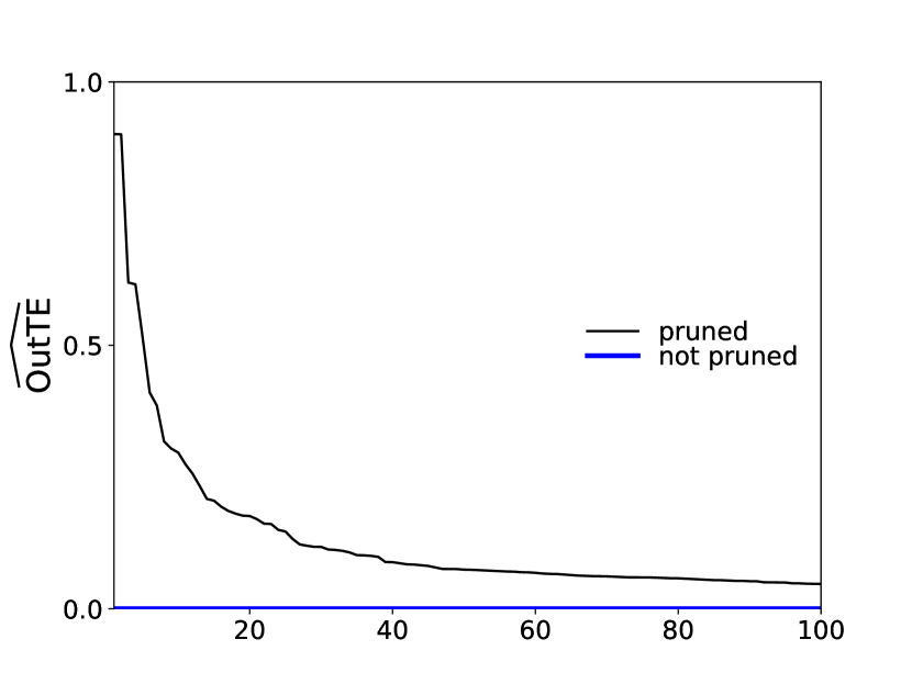
Figure 15: $\widehat{\rm OutTE}$ of OTUs in the saliva microbiota data, obtained with pruning, sorted in descending order of their values (black line) shown for top 100 OTUs, compared with estimates obtained without pruning (blue line).

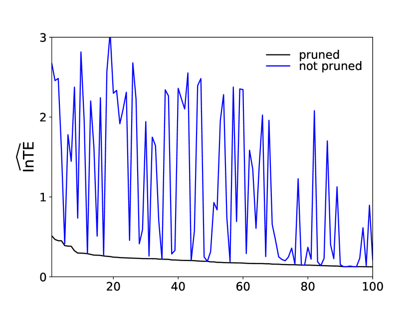
Figure 16: $\widehat{\rm InTE}$ of OTUs in the saliva microbiota data, obtained with pruning,sorted in descending order of their values (black line) shown for top 100 OTUs, compared with estimates obtained without pruning (blue line).

We now apply the current method to microbiota data obtained from a saliva sample observed for 226 days, consisting of 879 nodes, where each node represents an OTU [24]. The values of $\widehat{\rm OutTE}$ and $\widehat{\rm InTE}$ for all nodes are compared with and without pruning in Figs. 15 and  16, respectively, where the OTUs are sorted in descending order of estimates obtained with pruning. We observe that $\widehat{\rm OutTE}=0$ for all nodes without pruning, as mentioned earlier, whereas the values obtained with pruning vary between 0 and 0.9 (Fig. 15). In the case of $\widehat{\rm InTE}$, the estimated value is non-zero even without pruning. However, while the estimates obtained with pruning range between 0 and 0.5, those obtained without pruning can be as high as 3, and are unrelated to those obtained with pruning (Fig. 16), suggesting a large estimation error without pruning. Also, compared to $\widehat{\rm OutTE}$, where a few OTUs have very high values, such peaks are less pronounced for $\widehat{\rm InTE}$, where no values exceed 0.5. This difference in behavior can also be seen in the histograms, where 50 bins were used to count frequency of occurrence. The histogram of $\widehat{\rm OutTE}$ exhibits a power-law behavior (Fig. 15), whereas that of $\widehat{\rm InTE}$ fits the power-law less well (Fig. 16).

The top ten OTUs ranked by $\widehat{\rm OutTE}$ and $\widehat{\rm InTE}$ are shown in the table I. Some microbiota in the data are specified only at higher taxonomic levels. We find that two bacteria, Corynebacterium durum and Fusobacterium, stand out in terms of high $\widehat{\rm OutTE}$ values. C. durum is indeed known to play a crucial role in the community of oral microbiota. As a gram-positive bacterium, it is a prolific biofilm and extracellular matrix producer [30], and a decrease in this bacterium is associated with a disease [31]. Fusobacterium, particularly Fusobacterium nucleatum, is also well known as a key player in the community of oral bacteria [32, 33]. As a gram-negative bacterium, F. nucleatum is a major coaggregation bridge organism linking early and late colonizers in dental biofilm [34], and plays a role in carcinogenesis [35, 36]. No particular bacterium stands out in terms of $\widehat{\rm InTE}$ values. Furthermore, InTE measures vulnerability rather than influence, and it is unclear whether vulnerable species can be easily identified experimentally. Therefore, the biological relevance of the top microbiota in terms of $\widehat{\rm InTE}$ is less evident than for $\widehat{\rm OutTE}$.

Rank	OutTE		InTE
1	Corynebacterium Durum	0.90	Gemellales (order)	0.51
2	Fusobacterium (genus)	0.90	Oribacterium (genus)	0.47
3	Prevotella melaninogenica	0.62	Rothia mucilaginosa	0.45
4	Unknown	0.62	SR1 (phylum)	0.45
5	Coriobacteriaceae (family)	0.52	Flavobacterium succinicans	0.39

Table 1: Top ten microbiota with highest values of $\widehat{\rm OutTE}$ and $\widehat{\rm InTE}$.

V Conclusion

In this study, I introduced outgoing and incoming transfer entropy (OutTE and InTE) in interaction networks, as novel measures for quantifying causal influence of each component on the entire system and vice versa, aiming to identify the most influential (hub) and vulnerable (anti-hub) nodes. The new estimation method proposed here, which incorporates a pruning step to exclude unrelated nodes, significantly reduces estimation errors, particularly in scenarios where the number of variables approaches or exceeds the number of samples. This improvement is crucial for accurate causal inference in complex systems with numerous interacting components.

Through simulations using synthetic data, I demonstrated the effectiveness of the pruning-enhanced estimation method in accurately identifying the OutTE and InTE values. These results suggest that the method can reliably highlight key nodes in a network, providing valuable insights into the system’s dynamics. The application of this method to microbiota data from human saliva further validated its utility, successfully identifying bacterial species known to play critical roles in the oral microbiota community. Specifically, the identification of Corynebacterium durum and Fusobacterium as key players underscores the biological relevance of the OutTE measure in complex biological systems.

The proposed method offers a robust framework for the accurate estimation of causal influences in complex networks, with potential applications across various fields, including biology, neuroscience, and social sciences. Future work could focus on refining the causal network reconstruction algorithms to enhance the accuracy and efficiency of the initial pruning step. Additionally, applying this method to larger and more diverse datasets could further validate its utility and uncover new insights into the structure and function of complex systems.

Appendix A Proof of Nonnegativity of Various Information Theoretic Measures

Shannon entropy H quantifies uncertainty about the state of a system, defined as:

$${\rm H}(X)\equiv\left\langle-\log P(X)\right\rangle,$$ (10)

where the random variable $X$ represents the states of the system, and $P(X)$ denotes its probability distribution. footnoteHere the base of the log will be left arbitrary since the results does not depend on it. Since $P(X)$ is always less than or equal to one, we have $-\log P(X)\geq 0$, from which we get ${\rm H}(X)=\left\langle-\log P(X)\right\rangle\geq 0$.

The same argument applies to the conditional entropy $H(Y/X)$, as the conditional probability also satisfies the property of usual probability, $P_{Y/X}(y/x)\leq 1$, which results in:

$$H(Y/X)\equiv\left\langle-\log P(Y/X)\right\rangle\geq 0.$$ (11)

To prove the non-negativity of mutual information, we use Jensen’s inequality, which states that for any convex function $f(x)$ and any weights $p_{i}\ (i=1,\cdots m)$ (where $\sum_{i=1}^{m}p_{i}=1$), we have:

$$\sum_{i=1}^{m}p_{i}f(x_{i})\geq f(\sum_{i=1}^{m}p_{i}x_{i}).$$

Applying this inequaility to the convex function $f(x)=-\log(x)$, we get:

$$I(X,Y) = \sum_{x,y}P(X=x,Y=y)\left(-\log\frac{P(X=x)P(Y=y)}{P(X=x,Y=y)}\right)$$ (12)

$$\geq -\log\left(\sum_{x,y}P(X=x,Y=y)\frac{P(X=x)P(Y=y)}{P(X=x,Y=y)}\right)$$

$$= -\log\left(\sum_{x}P(X=x)\sum_{y}P(Y=y)\right)=0.$$

The same argument applies to conditional mutual information:

$$I(X,Y/Z) = \sum_{z}P(Z=z)\sum_{x,y}P(X=x,Y=y/Z=z)\left(-\log\frac{P(X=x/Z=z)P(Y=y/Z=z)}{P(X=x,Y=y/Z=z)}\right)$$ (13)

$$\geq 0,$$

where the last inequality follows by applying Eq. (12) for each $z$.

Since transfer entropy and conditional transfer entropy are conditional mutual information, they are all nonnegative.

Appendix B Underestimation of Conditional Entropy for Small Sample Sizes

Conditional entropy $H(Y/X)$ measures the amount of uncertainty remaining in a random variable $Y$ given that the value of another random variable $X$ is known. The true conditional entropy is defined as:

$$H(Y|X)=-\sum_{x}P(X=x)\sum_{y}P(Y=y|X=x)\log P(Y=y|X=x).$$

When estimating conditional entropy from a finite sample, the empirical conditional entropy $\hat{H}(Y/X)$ is calculated by substituting the true probabilities with their empirical estimates based on the observed data:

$$\hat{H}(Y/X)=-\sum_{x}\hat{P}(X=x)\sum_{y}\hat{P}(X=y|X=x)\log\hat{P}(X=y|X=x),$$

where empirical probabilities are calculated as:

$$\hat{P}(X=x)\equiv\frac{N(x)}{N},\quad\hat{P}(Y=y|X=x)\equiv\frac{N(x,y)}{N(x)}$$

with $N(x,y)$ being the number of times the pair $(x,y)$ occurs, and $N(x)$ the number of times $x$ occurs, and $N$ the total number of observations. In practice, the estimated conditional entropy $\hat{H}(Y|X)$ tends to be smaller than the true entropy $H(Y|X)$ when the sample size is small. This underestimation occurs due to insufficient observations, which leads to a biased estimation of probabilities.

The primary reason for the underestimation of conditional entropy lies in the concavity of the logarithm function and the bias introduced by finite sample sizes. Note that Jensen’s inequality can be written in the form

$$\langle f(X)\rangle\leq f(\langle X\rangle)$$ (14)

for any random variable $X$ and a concave function $f(x)$. The logarithm function $\log(x)$ is concave, which means that for any random variable $Z$:

$$\langle\log Z\rangle\leq\log\langle Z\rangle$$

In the context of conditional entropy, this inequality implies that the expected value of the logarithm of the estimated probability is less than the logarithm of the true probability. When probabilities are estimated from a small sample, the estimates $\hat{P}(Y=y|X=x)$ are typically more concentrated around zero for rare events, leading to a lower average entropy. That is, for small sample sizes, many possible pairs $(x,y)$ may not be observed at all, leading to $\hat{P}(Y=y|X=x)=0$ for these pairs. Since $\hat{P}(Y=y|X=x)\log\hat{P}(Y=y|X=x)$ is defined as $\lim_{p\to 0}p\log p=0$ when $\hat{P}(Y=y|X=x)=0$, this results in a lower estimated entropy. In contrast, the true probability $P(Y=y|X=x)$ might be nonzero, leading to a nonzero contribution to the true entropy $H(Y|X)$.

For example, consider a simple case where $X$ and $Y$ are binary variables, and the true conditional probabilities are:

$$P(Y=0|X=0)=1/2,\quad P(Y=1|X=0)=1/2$$

$$P(Y=0|X=1)=1/2,\quad P(Y=1|X=1)=1/2,$$

Suppose we have just two observations, with $(X,Y)=(0,0)$ and $(X,Y)=(1,1)$. The empirical conditional probabilities are:

$$\hat{P}(Y=0|X=0)=1,\quad\hat{P}(Y=1|X=0)=0$$

$$\hat{P}(Y=0|X=1)=0,\quad\hat{P}(Y=1|X=1)=1$$

The empirical conditional entropy $\hat{H}(Y|X)=0$ calculated from these estimates is less than the true conditional entropy $H(Y|X)=1$ calculated from the true probabilities, illustrating the underestimation bias.

Figure 1: The SR model with a sender node S and a receiver node R. The nodes ${\rm C}_{1},\cdots{\rm C}_{n}$ represent confounding nodes that are independent of the dynamics between S and R.

Figure 4: $\widehat{\rm InTE}(S)$ in the SR model as a function of $T$, for $n=0,3,6$ without pruning (black, blue, and green lines, respectively), and with pruning (red and orange lines for $n=0$ and $6$, respectively).

Figure 6: The HSAR model with a hub node H, a sender node S, an anti-hub node A, and a receiver node R. The nodes ${\rm C}_{1},\cdots{\rm C}_{n}$ represent confounding nodes that are independent of the dynamics among H, S, A, and R.

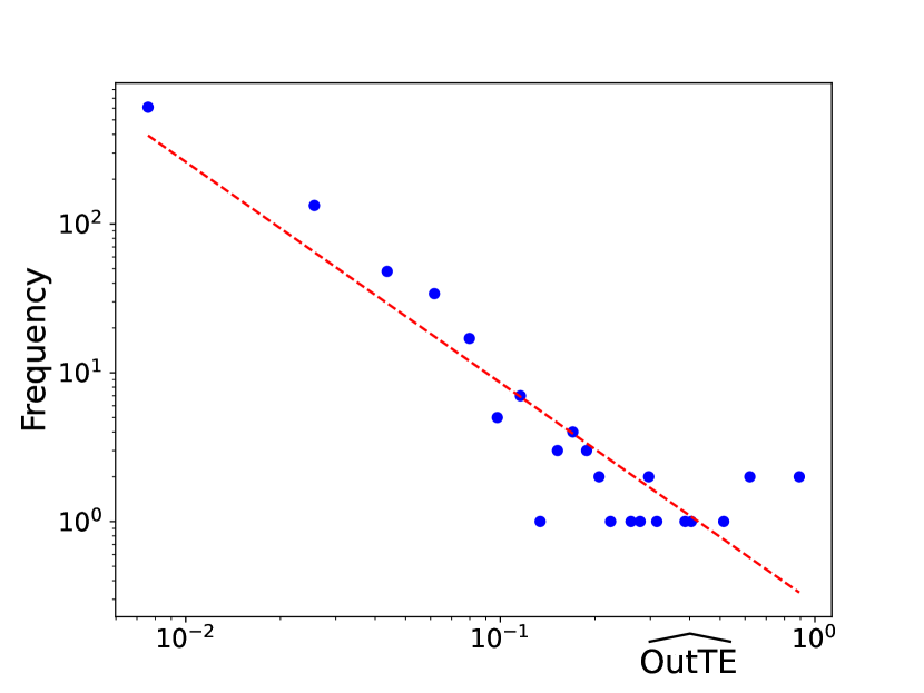
Figure 17: Histrogram of $\widehat{\rm OutTE}$ (blue filled circles) of OTUs in the saliva microbiota data, along with the a power law fit (red dashed line)

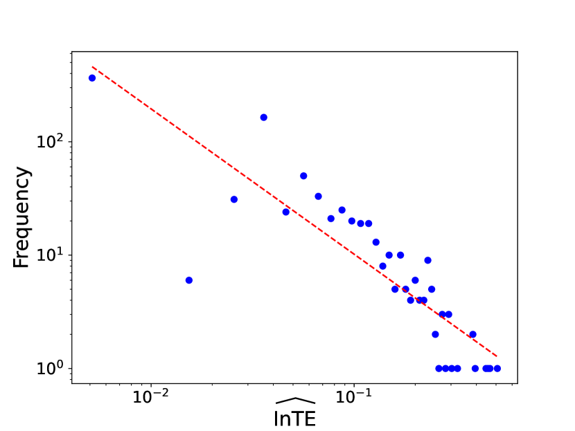
Figure 18: Histrogram of $\widehat{\rm INTE}$ (blue filled circles) of OTUs in the saliva microbiota data, along with the a power law fit (red dashed line)