Bayesian analysis of product feature allocation models

Abstract

Feature allocation models are an extension of Bayesian nonparametric clustering models, where individuals can share multiple features. We study a broad class of models whose probability distribution has a product form, which includes the popular Indian buffet process. This class plays a prominent role among existing priors, and it shares structural characteristics with Gibbs-type priors in the species sampling framework. We develop a general theory for the entire class, obtaining closed form expressions for the predictive structure and the posterior law of the underlying stochastic process. Additionally, we describe the distribution for the number of features and the number of hitherto unseen features in a future sample, leading to the $\alpha$-diversity for feature models. We also examine notable novel examples, such as mixtures of Indian buffet processes and beta Bernoulli models, where the latter entails a finite random number of features. This methodology finds significant applications in ecology, allowing the estimation of species richness for incidence data, as we demonstrate by analyzing plant diversity in Danish forests and trees in Barro Colorado Island.

Keywords: Bayesian nonparametrics, completely random measures, exchangeable feature probability function, Gibbs-type feature models, Indian buffet process

1 Introduction

Random feature allocations have emerged as an important area of Bayesian nonparametrics. The pioneering work of Griffiths and Ghahramani (2006) introduced the Indian buffet process (ibp), a stochastic mechanism for binary matrices, which is obtained by considering the infinite limit of a beta Bernoulli (bb) model. Unlike clustering problems, where each individual belongs to a single group, in feature allocation models every observation may possess a finite set of features or attributes. Shortly after its proposal, Thibaux and Jordan (2007) demonstrated that de Finetti’s celebrated theorem could be applied to the ibp, establishing its connection to the beta process of Hjort (1990). This pivotal finding linked ibps to the theory of completely random measures (Kingman, 1967), laying the groundwork for a new branch of Bayesian nonparametrics. These initial investigations sparked a rich stream of research, particularly within the machine learning community. ibp models have found widespread applicability across various domains, including Bayesian factor analysis and nonnegative matrix factorization (Griffiths and Ghahramani, 2006; Knowles and Ghahramani, 2011; Ayed and Caron, 2021), topic modeling (Williamson et al., 2010), relational models (Miller et al., 2009; Palla et al., 2012), and object recognition (Broderick et al., 2015). We refer to Teh and Jordan (2010) and Griffiths and Ghahramani (2011) for a comprehensive review of the early contributions. The relevance of ibps as a statistical tool is now firmly established; however, their limitations have also become apparent, as well as the need for a deeper theoretical understanding. For example, the logarithmic growth rate of the number of features in the two-parameter ibp (Griffiths and Ghahramani, 2011) spurred the proposal of a three-parameter generalization by Teh and Gorur (2009), which exhibits a power-law behavior; see also Broderick et al. (2012). Another major step was pursued by Broderick et al. (2013), who showed that most feature models are characterized by a combinatorial entity known as the exchangeable feature probability function (efpf). More recently, James (2017) studied a general class of feature models based on completely random measures, while another extensive class, relying on random scaling of the underlying process, is investigated in Camerlenghi et al. (2024). Another recent construction is discussed in Heaukulani and Roy (2020).

In this paper, we study the broad class of feature models defined by Battiston et al. (2018), who holds the merit of characterizing all efpfs with a product form as mixtures of the two most widely used feature models, namely the Indian buffet process (ibp, Teh and Gorur, 2009) and the beta Bernoulli (bb, Griffiths and Ghahramani, 2006). However, apart from this important representation theorem, a comprehensive statistical investigation is still lacking. We develop a general theory for this class of models, encompassing (i) the predictive structure, leading to a generalized Indian buffet metaphor, (ii) the posterior distribution of the underlying process, (iii) prior and posterior properties regarding the number of features, and (iv) the asymptotic behavior. Our findings are available in closed form, lead to computationally efficient inferential procedures, and enjoy a transparent interpretation. Moreover, this theoretical investigation allows us to identify three novel feature allocation models that stand out for their tractability: the gamma mixture of ibps, and the Poisson and negative binomial mixture of bbs. The latter two models entail a random but finite number of possible features, therefore being structurally different from existing ibp-like specifications that involve infinitely many features. Finally, we highlight several remarkable parallelisms between the class of Battiston et al. (2018) and Gibbs-type priors for species sampling models (Gnedin and Pitman, 2005; De Blasi et al., 2015). In light of these similarities, we will refer to this class as Gibbs-type feature models. In species sampling problems, Gibbs-type priors are perhaps the most natural generalization of the Dirichlet process of Ferguson (1973), owing to their balance between flexibility and analytical tractability. Notable examples are the Pitman–Yor process (Pitman and Yor, 1997), the normalized generalized gamma process (Lijoi et al., 2007b), and mixtures of Dirichlet multinomial processes (Gnedin, 2010; De Blasi et al., 2013). For similar reasons, we argue that Gibbs-type feature models are one of the most natural extensions of the ibp and the bb.

We demonstrate here the usefulness of feature models in ecological problems as a tool to measure biodiversity. There exists a rich literature about the quantification of biodiversity (Colwell, 2009; Magurran and McGill, 2011) with taxon richness, i.e., the number of different taxa present in a community, being perhaps the simplest and most natural definition. Richness estimation is, in turn, related to the notion of taxon accumulation curves (Gotelli and Colwell, 2001). A Bayesian nonparametric inferential framework for predicting unseen species has been laid down by Lijoi et al. (2007a) for Gibbs-type priors. See also Favaro et al. (2009) for the Pitman–Yor special case and Zito et al. (2023a) for a related model-based approach. These Bayesian methods are suitable for individual-based accumulation curves, that is, when species are observed one at a time. However, species are often captured or collected in chunks, and hence, each observation takes the form of a vector of binary variables accounting for the presence or absence of a species. Feature models are well-suited for this kind of data, called incidence data, leading to a Bayesian analysis of sample-based accumulation curves. Despite the development of classical estimators for this setting (e.g. Colwell et al., 2012; Chiu et al., 2014; Chao et al., 2014; Chakraborty et al., 2019; Chiu, 2022, 2023), the Bayesian nonparametric literature remains much more limited, except for the recent works of Masoero et al. (2022); Camerlenghi et al. (2024). Our theoretical investigation allows for the prediction of the number of unseen species, the modeling of accumulation curves, and the quantification of biodiversity. For instance, an important theoretical result of this paper, particularly relevant for ecological applications, is the definition of the $\alpha$-diversity, a biodiversity measure that extends the notion of Pitman (2003) to sample-based designs. In the proposed Poisson and negative binomial mixture of bb models, the $\alpha$-diversity coincides with the taxon richness, and its posterior distribution follows a Poisson and a negative binomial distribution, respectively. This leads to straightforward Bayesian estimators for the taxon richness whose uncertainty can be formally and easily quantified.

The paper is structured as follows. In Section 2, we review feature allocation models. In Section 3 we develop general theory for the class of Gibbs-type feature models. In Sections 4-5 we propose and study novel examples of Gibbs-type feature allocation models, distinguishing between models with an infinite number of features (mixtures of ibps) and those assuming finitely many features (mixtures of bbs). Simulation studies are discussed in Section 6, while Section 7 illustrates our methodology by analyzing two real datasets. The paper ends with a discussion; proofs, additional theorems, and simulation studies are collected in the supplementary material.

2 Feature allocation models

2.1 Preliminary concepts

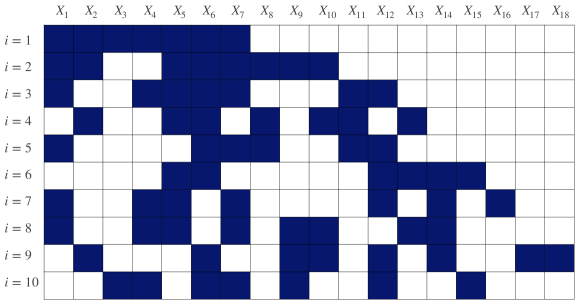
Figure 1: Matrix representation of a feature allocation, with $n=10$ individuals and $K_{n}=18$ observed features. Features are in order of appearance (Broderick et al., 2013). The blue squares correspond to $A_{i,\ell}=1$ (the $i$th individual displays feature $X_{\ell}$), the white squares correspond to $A_{i,\ell}=0$ (the $i$th does not express feature $X_{\ell}$).

Feature allocation models describe how features are distributed among a sample of $n$ individuals (Broderick et al., 2013). Let $[n]=\{1,\ldots,n\}$ be a set comprising the first $n$ natural numbers. An ordered feature allocation is a sequence of non-empty sets $B_{n,\ell}\subseteq[n]$, for $\ell=1,\ldots,K_{n}$, such that $B_{n,\ell}$ identifies the set of individuals exhibiting the $\ell$th feature. To distinguish these sets, we assign them a label. More precisely, suppose $\mathds{X}$ is the space of feature labels, and let $X_{\ell}\in\mathds{X}$ be the label associated with the set $B_{n,\ell}$, for $\ell=1,\ldots,K_{n}$. The labels $X_{\ell}$ are independent and identically distributed (i.i.d.) draws, that is $X_{\ell}\stackrel{{\scriptstyle\textup{iid}}}{{\sim}}P_{0}$, with $P_{0}$ being a diffuse distribution on $\mathds{X}$, ensuring that the labels are almost surely (a.s.) distinct. The association between feature allocations and labels can be encoded using binary random variables $A_{i,\ell}$ for $i=1,\dots,n$ and $\ell=1,\dots,K_{n}$, so that $A_{i,\ell}$ equals $1$ if the $i$th individual displays feature $X_{\ell}$ and $0$ otherwise. In other terms, the random set $B_{n,\ell}$ may be written as $B_{n,\ell}=\{i\in[n]:A_{i,\ell}=1\}$. A feature allocation can be represented through binary matrices, as depicted in Figure 1, where there are $n=10$ individuals and $K_{n}=18$ features. Each column of the binary matrix corresponds to a set $B_{n,\ell}$, with the $i$th element of the $\ell$th column representing the value $A_{i,\ell}$. We assume that each individual may exhibit only a finite number of features; that is, an individual belongs to a finite number of $B_{n,\ell}$’s. This implies that the total number of observed features $K_{n}$ is a.s. finite for any $n\geq 1$.

A feature allocation model is a probability distribution for a random ordered feature allocation $F_{n}=(B_{n,1},\dots,B_{n,K_{n}})$. Alternatively, one may consider the probability distribution for an unordered feature allocation $\tilde{F}_{n}=\{(\tilde{B}_{n,1},\tilde{K}_{n,1}),\ldots,(\tilde{B}_{n,H_{n}},\tilde{K}_{n,H_{n}})\}$, where $\tilde{B}_{n,h}\subseteq[n]$ are the $H_{n}\leq K_{n}$ distinct sets among the $B_{n,1},\ldots,B_{n,K_{n}}$, with $\tilde{K}_{n,h}$ being the number of sets equal to $\tilde{B}_{n,h}$. The unordered $\tilde{F}_{n}$ is sometimes used to define feature allocation models (see Broderick et al., 2013), but for our purposes, it is more convenient to deal with the ordered $F_{n}$. In any event, we assume that the probability of $\tilde{F}_{n}$ being equal to any unordered feature allocation $\tilde{f}_{n}$ is equally split between the $K_{n}!/\prod_{h=1}^{H_{n}}\tilde{K}_{n,h}!$ possible orders of the sets $B_{n,1},\ldots,B_{n,K_{n}}$. Hence, the following relationship holds

$$\mathds{P}(\tilde{F}_{n}=\tilde{f}_{n})=\frac{{K_{n}}!}{\prod_{h=1}^{H_{n}}\tilde{K}_{n,h}!}\mathds{P}(F_{n}=f_{n}),$$

where $f_{n}$ is one of the possible orderings of $\tilde{f}_{n}$.

In this paper, we focus on feature allocation models admitting an exchangeable feature probability function (efpf). This is a probabilistic object whose role is analogous to the exchangeable partition probability function (eppf) in the species sampling framework (Pitman, 1996), as carefully discussed in Broderick et al. (2013). Specifically, let $(M_{n,1},\ldots,M_{n,K_{n}})$ be the random vector of feature frequencies, where $M_{n,\ell}=\#B_{n,\ell}=\sum_{i=1}^{n}{A_{i,\ell}}$, for $\ell=1,\ldots,K_{n}$. We assume that the probability distribution of $F_{n}$ depends on the sample solely through the vector $\bm{M}^{(n)}=(M_{n,1},\ldots,M_{n,K_{n}})$, namely

$$\mathds{P}(F_{n}=f_{n})=\pi_{n}(m_{1},\ldots,m_{k}),$$

for every $f_{n}$ and for every $n\geq 1$, where $\pi_{n}$ is a $[0,1]$-valued symmetric function defined on $\bigcup_{k\geq 0}[n]^{k}$, and $(m_{1},\ldots,m_{k})$ are the feature frequencies for $f_{n}$. The function $\pi_{n}$ is termed exchangeable feature probability function, and it encapsulates all the relevant properties of the model. By construction, feature allocation models admitting an efpf are exchangeable, meaning that the distribution of $F_{n}$ is invariant under any permutation of the indexes of the $n$ individuals. It is also natural to require feature models to be Kolmogorov consistent, which means that the probability distribution of the feature allocation for $n$ individuals coincides with that for $n+1$ individuals once the last individual is integrated out. We refer to Broderick et al. (2013) for a detailed discussion.

2.2 Exchangeable Gibbs-type feature allocation models

Among the exchangeable and consistent models, the class of efpf in product form introduced by Battiston et al. (2018) represents a special subset that is still very rich and diversified. We refer to this class as exchangeable Gibbs-type feature allocation models, or Gibbs-type feature models for brevity, for the evident similarity with exchangeable Gibbs-type random partitions (Gnedin and Pitman, 2005). We consider efpfs of the following product form $\pi_{n}(m_{1},\ldots,m_{k})=V_{n,k}\prod_{\ell=1}^{k}W_{m_{\ell}}U_{n-m_{\ell}}$, where $V=(V_{n,k}:(n,k)\in\mathds{N}\times\mathds{N}_{0})$ and $W=(W_{j}:j\in\mathds{N})$, $U=(U_{j}:j\in\mathds{N}_{0})$ are two sequences of non-negative weights, with $\mathds{N}$ denoting the set of natural numbers and $\mathds{N}_{0}=\mathds{N}\cup\{0\}$. Apart from some limiting cases, an important result of Battiston et al. (2018) states that Gibbs-type feature models are necessarily of the form

$$\pi_{n}(m_{1},\ldots,m_{k})=V_{n,k}\prod_{\ell=1}^{k}(1-\alpha)_{m_{\ell}-1}(\theta+\alpha)_{n-m_{\ell}},$$ (1)

for $-\infty<\alpha<1$ and $-\alpha<\theta<\infty$, where $(x)_{m}=\Gamma(x+m)/\Gamma(x)$ is the Pochhammer symbol, and $\Gamma(x)$ is the gamma function. The array $V$ must satisfy the following recurrence relationship $V_{n,k}=\sum_{j=0}^{\infty}(k+j)!/\{j!k!\}\{(\theta+\alpha)_{n}\}^{j}(\theta+n)^{k}V_{n+1,k+j}$, which guarantees the consistency of the efpf. The limiting case $\alpha=1$ corresponds to no feature sharing, i.e., $M_{n,\ell}=1$ almost surely for $\ell=1,\dots,K_{n}$, whereas $\theta=-\alpha$ corresponds to complete feature sharing, that is $M_{n,\ell}=n$ almost surely, for $\ell=1,\dots,K_{n}$. These degenerate situations are uninteresting in practice.

The most popular and widely used feature allocation models are of Gibbs-type. A first noteworthy example is the three-parameter Indian buffet process (ibp), introduced in Teh and Gorur (2009), with parameters $(\gamma,\alpha,\theta)$ satisfying $\gamma>0$, $0\leq\alpha<1$, and $\theta>-\alpha$. The efpf is in product form (1) and the $V_{n,k}$’s are given by

$$V_{n,k}=\frac{1}{k!}\left\{\frac{\gamma}{(\theta+1)_{n-1}}\right\}^{k}\exp\left\{-\gamma g_{n}(\theta,\alpha)\right\},\quad\text{with}\quad g_{n}(\theta,\alpha):=\sum_{i=1}^{n}\frac{(\theta+\alpha)_{i-1}}{(\theta+1)_{i-1}}.$$ (2)

The choice $\alpha=0$ corresponds to the two-parameter ibp, while the one-parameter model is obtained by further considering $\theta=1$; see Griffiths and Ghahramani (2011). We stress that the distribution of $K_{n}$, in the ibp case, has unbounded support. A second notable example is the beta Bernoulli (bb), with parameters $(N,\alpha,\theta)$ such that $N\in\mathds{N}$, $\alpha<0$ and $\theta>-\alpha$ (Griffiths and Ghahramani, 2011). The efpf of a bb is also in product form (1), with the $V_{n,k}$’s given by

$$V_{n,k}=\binom{N}{k}\left\{\frac{-\alpha}{(\theta+\alpha)_{n}}\right\}^{k}\left\{\frac{(\theta+\alpha)_{n}}{(\theta)_{n}}\right\}^{N}\mathds{1}_{\{0,1,\ldots,N\}}(k),$$ (3)

where $\mathds{1}_{C}$ denotes the indicator function of a set $C$. The bb model prescribes that the observed number of features $K_{n}$ is bounded by $N$. Remarkably, a characterization theorem due to Battiston et al. (2018) establishes that the ibp and the bb are the building blocks of any Gibbs-type feature model. More precisely, for fixed values of $(\theta,\alpha)$, the set of Gibbs coefficients $V_{n,k}$ satisfying the aforementioned consistency condition are necessarily mixtures of the $\gamma$ and $N$ parameters of the ibp and the bb, respectively. This is better clarified in the following result.

Proposition 1 (Theorem 1.1 of Battiston et al. (2018)).

For fixed values of $(\theta,\alpha)$ such that $\theta>-\alpha$, the set of solutions of the recursions for the $V_{n,k}$’s is:

• for $0\leq\alpha<1$, mixtures over $\gamma\in\mathds{R}^{+}$ of the $V_{n,k}$’s of ibps with respect to a distribution $P_{\gamma}$;

• for $\alpha<0$, mixtures over $N\in\mathds{N}$ of the $V_{n,k}$’s of bbs with respect to a distribution $P_{N}$.

Hence, any Gibbs-type feature model is obtained by considering a prior distribution for the $\gamma$ and $N$ parameters of the ibp and bb models. This draws an elegant parallelism between Gibbs-type feature models and Gibbs-type partitions of Gnedin and Pitman (2005) since, in both cases, product form distributions are obtained as mixtures of a set of simple models. These analogies will be strengthened in Section 3, where we will show that the parameter $\alpha$ also controls the asymptotic growth rate for the number of distinct features $K_{n}$, as in species sampling models, leading to the analogous of the $\alpha$-diversity of Pitman (2003) for feature allocations.

2.3 Hierarchical representations and random measures

Gibbs-type feature models admit a hierarchical representation in terms of Bernoulli processes (bps) and random measures. For the two-parameter ibp, such a stochastic representation was established in the illuminating contribution of Thibaux and Jordan (2007). Let us consider the sequence of all possible feature labels $(\tilde{X}_{j})_{j\geq 1}$, where $\tilde{X}_{j}\stackrel{{\scriptstyle\textup{iid}}}{{\sim}}P_{0}$ for any $j\geq 1$. The labels $X_{1},\dots,X_{K_{n}}$ observed in a sample of $n$ individuals are a subset of the complete list of labels $(\tilde{X}_{j})_{j\geq 1}$. The $i$th individual is characterized by its expressed features, i.e., by the pairs $((\tilde{X}_{j},\tilde{A}_{i,j}))_{j\geq 1}$, where each $\tilde{A}_{i,j}=1$ if the $i$th individual exhibits feature $\tilde{X}_{j}$, and $\tilde{A}_{i,j}=0$ otherwise. Thus, the pairs $((\tilde{X}_{j},\tilde{A}_{i,j}))_{j\geq 1}$ may be organized through a counting measure $Z_{i}$ on the space $\mathds{X}$, which is given by

$$Z_{i}(\cdot)=\sum_{j\geq 1}\tilde{A}_{i,j}\delta_{\tilde{X}_{j}}(\cdot).$$ (4)

The feature allocation $F_{n}=(B_{n,1},\ldots,B_{n,K_{n}})$ and the binary variables $A_{i,\ell}$ can be then expressed through the counting measures $Z_{i}$, since we have $B_{n,\ell}=\{i\in[n]:Z_{i}(\{X_{\ell}\})=1\}$ and $A_{i,\ell}=Z_{i}(\{X_{\ell}\})$.

In Gibbs-type feature models, the $\tilde{A}_{i,j}$’s are conditionally independent Bernoulli random variables given a sequence of random probabilities $(\tilde{q}_{j})_{j\geq 1}$ such that $\sum_{j\geq 1}\tilde{q}_{j}<\infty$ almost surely. In other terms, we suppose that $\tilde{A}_{i,j}\mid\tilde{q}_{j}\stackrel{{\scriptstyle\textup{ind}}}{{\sim}}\text{Bernoulli}(\tilde{q}_{j})$. We organize these probabilities using another measure $\tilde{\mu}$ on $\mathds{X}$, namely

$$\tilde{\mu}(\cdot):=\sum_{j\geq 1}\tilde{q}_{j}\delta_{\tilde{X}_{j}}(\cdot).$$ (5)

We will say that, conditionally on $\tilde{\mu}$, the $Z_{i}$’s are i.i.d. Bernoulli processes with base measure $\tilde{\mu}$, written $Z_{i}\mid\tilde{\mu}\stackrel{{\scriptstyle\textup{iid}}}{{\sim}}\textsc{bp}(\tilde{\mu})$ for any $i\geq 1$. Hence, the infinite sequence of random measures $(Z_{i})_{i\geq 1}$ is exchangeable by virtue of de Finetti’s theorem (de Finetti, 1937). Summarizing, the following hierarchical representation holds:

$$\begin{split}Z_{i}\mid\tilde{\mu}&\stackrel{{\scriptstyle\mbox{\scriptsize{iid}}}}{{\sim}}\textsc{bp}(\tilde{\mu}),\qquad i\geq 1,\\ \tilde{\mu}&\sim Q,\end{split}$$ (6)

where $Q$ is the prior distribution of $\tilde{\mu}$, i.e., the de Finetti measure. The hierarchical generative scheme outlined in equations (4)-(5)-(6) is termed a feature frequency model, and it leads to a consistent and exchangeable efpf (Broderick et al., 2013). Gibbs-type feature models always admit such a hierarchical construction under specific prior distributions for the random measure $\tilde{\mu}$. This is a well-known fact for ibp and bb models, whose random measures are denoted by $\tilde{\mu}\mid\gamma$ and $\tilde{\mu}\mid N$. Hence, thanks to Proposition 1, the law of $\tilde{\mu}$ for any Gibbs-type feature model is a mixture over $\gamma$ or $N$ of the corresponding law for the ibp or bb model.

Let us firstly consider the bb model with parameters $(N,\alpha,\theta)$, in which there are $N$ possible features $\tilde{X}_{1},\dots,\tilde{X}_{N}$. The hierarchical representation of the beta Bernoulli process is straightforward as we have $\tilde{\mu}\mid N=\sum_{j=1}^{N}\tilde{q}_{j}\delta_{\tilde{X}_{j}}$, with $\tilde{q}_{j}\stackrel{{\scriptstyle\textup{iid}}}{{\sim}}{\rm Beta}(-\alpha,\theta+\alpha)$ and $\tilde{X}_{j}\stackrel{{\scriptstyle\textup{iid}}}{{\sim}}P_{0}$, for $j=1,\ldots,N$, recalling that $\alpha<0$ and $\theta>-\alpha$. See Lemma S4 in the supplementary material for a precise statement of this simple fact. The construction of the ibp, on the other hand, is more elaborate, and it involves infinitely many labels $\tilde{X}_{j}$ and probabilities $\tilde{q}_{j}$. Let us define the class of homogeneous completely random measures (crms, Kingman, 1967) without fixed atoms, which are characterized by a Laplace functional of the following type

$$\mathds{E}[e^{-\int_{\mathds{X}}f(x)\tilde{\mu}({\rm d}x)}]=\exp\left\{-\int_{\mathds{X}}\int_{0}^{\infty}\left[1-e^{-sf(x)}\right]\rho({\rm d}s)P_{0}({\rm d}x)\right\},$$

for any measurable function $f:\mathds{X}\to\mathds{R}_{+}$, where $\rho(\mathrm{d}s)$ is an intensity measure on $\mathds{R}_{+}$, identifying the distribution of the probabilities $(\tilde{q}_{j})_{j\geq 1}$, and $P_{0}$ is a diffuse distribution on $\mathds{X}$ from which the labels $\tilde{X}_{j}$ are sampled. We will write $\tilde{\mu}\sim\textsc{crm}(\rho;P_{0})$. We refer to Daley and Vere-Jones (2008) for a mathematical treatment of crms and Lijoi and Prünster (2010) for a presentation of crms as a unifying concept in Bayesian nonparametrics. In model (6) the random measure $\tilde{\mu}$ must have jumps $\tilde{q}_{j}\in(0,1)$, hence we require the intensity measure $\rho({\rm d}s)$ of the crm to be supported in $(0,1)$. As shown in Teh and Gorur (2009), in the ibp the measure $\tilde{\mu}\mid\gamma$ is distributed as a completely random measure and, more precisely, it follows a stable-beta process, whose intensity measure $\rho({\rm d}s)$ is

$$\rho(\mathrm{d}s)=\gamma\frac{\Gamma(1+\theta)}{\Gamma(1-\alpha)\Gamma(\theta+\alpha)}s^{-\alpha-1}(1-s)^{\theta+\alpha-1}{\rm d}s.$$ (7)

Note that $\gamma$ is sometimes called the total mass parameter because $\gamma=\mathds{E}\left[{\tilde{\mu}}(\mathds{X})\right]=\sum_{j\geq 1}\mathds{E}\left[\tilde{q}_{j}\right]$ is the expected sum of all the probabilities. The choice $\alpha=0$ leads to the beta process of Hjort (1990), as it was established by Thibaux and Jordan (2007). There exist several sampling strategies for the weights $\tilde{q}_{j}\in(0,1)$, for example based on size-biased constructions or the inverse of the Lévy measure (Teh and Gorur, 2009). Alternative and more recent approaches include stick-breaking representations (Broderick et al., 2012), or independent finite approximations (Lee et al., 2023; Nguyen et al., 2023).

3 Predictive structure of Gibbs-type feature models

3.1 A buffet metaphor for Gibbs-type feature models

We begin our theoretical investigation of Gibbs-type feature models by presenting the predictive distribution for the $(n+1)$th individual, given a sample of $n$ data points. In the notation of Section 2.3, we study the conditional distribution of $Z_{n+1}$, given a random sample $\bm{Z}^{(n)}=(Z_{1},\dots,Z_{n})$, where the latter entails $K_{n}=k$ observed features $X_{1},\ldots,X_{k}$ whose presence is encoded by the binary variables $A_{i,\ell}$’s. The relevant aspects of the distribution of $Z_{n+1}$ are conveyed by the vector of random variables $(Y_{n+1},A_{n+1,1},\ldots,A_{n+1,k})$ such that: (i) $Y_{n+1}$ is the number of new features displayed by the $(n+1)$th individual, i.e., the features hitherto unobserved in the sample $\bm{Z}^{(n)}$; (ii) each $A_{n+1,\ell}$ is a binary random variable such that $A_{n+1,\ell}=1$ if the $(n+1)$th individual displays feature $X_{\ell}$ and $A_{n+1,\ell}=0$ otherwise. Our first key result provides the predictive law of Gibbs-type feature models, i.e., the probability distribution

$$p_{n+1}(y,a_{1},\ldots,a_{k}):=\mathds{P}((Y_{n+1},A_{n+1,1},\ldots,A_{n+1,k})=(y,a_{1},\ldots,a_{k})\mid\bm{Z}^{(n)}).$$

We will write $\mathscr{B}(a;p)=p^{a}(1-p)^{1-a}$ to denote the probability mass function of a Bernoulli random variable with parameter $p\in(0,1)$ evaluated at $a\in\{0,1\}$.

Theorem 1 (Predictive law).

Suppose the efpf is in product form (1), then the predictive law is

$$p_{n+1}(y,a_{1},\ldots,a_{k})=\binom{k+y}{k}\frac{V_{n+1,k+y}}{V_{n,k}}\{(\theta+\alpha)_{n}\}^{y}(\theta+n)^{k}\prod_{\ell=1}^{k}\mathscr{B}\left(a_{\ell};\frac{m_{\ell}-\alpha}{\theta+n}\right).$$

An important remark is in order: given the sample $\bm{Z}^{(n)}$, the random variable $Y_{n+1}$ is independent on the binary random variables $A_{n+1,1},\ldots,A_{n+1,k}$, which are also mutually independent. This is a consequence of the product form representation (1). In the second place, the count $Y_{n+1}$ of new features depends on the sample $\bm{Z}^{(n)}$ through the sample size $n$ and the number of observed features $K_{n}=k$, but not the frequencies $m_{1},\dots,m_{k}$. It is also noteworthy that what distinguishes Gibbs-type feature models is only the distribution of the number of new features $Y_{n+1}$. In fact, the probability distribution of the variables referring to the previously observed features, $A_{n+1,1},\ldots,A_{n+1,k}$, is common to all Gibbs-type feature models and does not depend on the chosen set of $V_{n,k}$’s. We will provide more precise comments on the distribution of $Y_{n+1}$ when presenting specific examples in Sections 4–5.

As an immediate consequence of Theorem 1, one can easily determine the probability that the $(n+1)$th individual does not exhibit new features. Such a probability may be interpreted as a sample-based version of the sample coverage (Good, 1953; Good and Toulmin, 1956), that is, the probability of re-observing a feature among those in the sample. However, it is worth noting that other definitions of sample coverage have been proposed in the feature setting; see, for example, Chiu (2023) and references therein.

Corollary 1 (Sample coverage).

Suppose the efpf is in product form (1), then the probability that $Z_{n+1}$ does not show any new features, given $\bm{Z}^{(n)}$, is

$$\mathds{P}(``Z_{n+1}\text{ has no new features}"\mid\bm{Z}^{(n)})=\mathds{P}(Y_{n+1}=0\mid\bm{Z}^{(n)})=\frac{V_{n+1,k}}{V_{n,k}}(\theta+n)^{k}.$$

The predictive distribution presented in Theorem 1 can be likened to the Indian buffet metaphor (Griffiths and Ghahramani, 2011). Our metaphor imagines a scenario where “customers”, representing individuals, sequentially enter a restaurant and select a number of “dishes”, corresponding to feature labels $(\tilde{X}_{j})_{j\geq 1}$, as depicted in Figure 2. Each customer has the option to choose from previously ordered dishes or select new ones. For any Gibbs-type feature model, the generative process unfolds as follows: the first customer enters the restaurant and selects $Y_{1}$ dishes according to the distribution

$$\mathds{P}(Y_{1}=y)=V_{1,y},$$

and $K_{1}=Y_{1}$. The $K_{1}$ selected dishes are associated with labels $X_{\ell}$, for $\ell=1,\ldots,K_{1}$, provided that $K_{1}>0$. Then, the $(n+1)$th customer enters and selects dishes in two steps. Firstly, the customer picks $Y_{n+1}$ new dishes (not chosen by the previous $n$ customers) according to the distribution

$$\mathds{P}(Y_{n+1}=y\mid K_{n})=\binom{k+y}{k}\frac{V_{n+1,k+y}}{V_{n,k}}\{(\theta+\alpha)_{n}\}^{y}(\theta+n)^{k},$$

where $K_{n}=k$ denotes the number of distinct dishes chosen by the first $n$ customers, so that $K_{n+1}=K_{n}+Y_{n+1}$. If $Y_{n+1}>0$, then the new dishes are associated with labels $X_{\ell}$, for $\ell=K_{n}+1,\ldots,K_{n+1}$. Secondly, the $(n+1)$th customer may select some of the previously chosen dishes $X_{1},\dots,X_{k}$ as encoded by the binary variables $A_{n+1,1},\ldots,A_{n+1,k}$, whose distribution is

$$A_{n+1,\ell}\mid\bm{Z}^{(n)}\stackrel{{\scriptstyle\mbox{\scriptsize{ind}}}}{{\sim}}{\rm Bernoulli}\left(\frac{m_{\ell}-\alpha}{\theta+n}\right),$$ (8)

where $m_{\ell}$ corresponds to the number of previous customers who selected dish $X_{\ell}$. Higher values of $m_{\ell}$ correspond to a higher probability of dish $X_{\ell}$ being selected again.

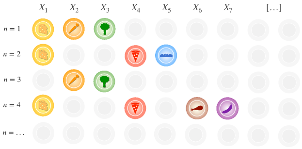
Figure 2: The buffet metaphor for Gibbs-type feature models. In this example there are $n=4$ customers and $K_{n}=7$ dishes. The observed frequencies of the dishes are $(m_{1},\dots,m_{7})=(3,2,2,2,1,1,1)$. The numbers of new dishes picked by each customer (from top to bottom) are $Y_{1}=3$, $Y_{2}=2$, $Y_{3}=0$, and $Y_{4}=2$.

This general buffet metaphor provides a simple sampling strategy for any Gibbs-type feature allocation model; moreover, it offers a clear interpretation for the parameters $\theta$ and $\alpha$. Essentially, the posterior probability of observing the $\ell$th feature can be viewed as the weighted combination of two factors: one representing the observed data and the other reflecting prior beliefs, akin to a typical Bayesian updating rule. Specifically, for $\ell=1,\dots,k$:

$$\mathds{P}(A_{n+1,\ell}=1\mid\bm{Z}^{(n)})=\frac{m_{\ell}-\alpha}{\theta+n}=\hat{p}_{\ell}\frac{n}{\theta+n}+\left(-\frac{\alpha}{\theta}\right)\frac{\theta}{\theta+n},$$

where $\hat{p}_{\ell}=m_{\ell}/n$ denotes the empirical frequency of the $\ell$th observed feature. When $\alpha<0$, the quantity $-\alpha/\theta\in(0,1)$ can be conveniently interpreted as the prior frequency of a feature, while $\theta$ assumes the familiar role of prior sample size. Small values of $\theta>0$ suggest low confidence in the prior guess, and vice versa. In cases where $\alpha\in[0,1)$, $\theta$ continues to control the relevance of prior beliefs, while $-\alpha/\theta$ determines the extent of (potentially negative) shrinkage on the probability of re-observing an old feature.

Finally, we point out that the buffet metaphor for the ibp, also discussed in Teh and Gorur (2009), emerges as a special case. In the ibp, the predictive process is characterized by $Y_{1}\mid\gamma\sim\textup{Poisson}(\gamma)$ and $Y_{n+1}\mid K_{n},\gamma\sim\textup{Poisson}\left(\gamma(\theta+\alpha)_{n}/(\theta+1)_{n}\right)$ for $n\geq 1$. Moreover, as can be verified via Theorem 1 using $V_{n,k}$ from (3), the bb model leads to $Y_{1}\mid N\sim\textup{Binomial}\left(N,-\alpha/\theta\right)$ and $Y_{n+1}\mid K_{n},N\sim\textup{Binomial}\left(N-k,-\alpha/(\theta+n)\right)$, where $\textup{Binomial}(n_{0},p)$ denotes a binomial random variable with parameters $n_{0}\in\mathds{N}$ and $p\in(0,1)$. Consequently, in a bb model, no new features can be displayed once $K_{n}=N$ features are observed.

3.2 Distribution of the number of features

We now investigate distributional properties of $K_{n}$, the total number of distinct features observed in a sample of size $n$. Note that we can also express $K_{n}$ as $Y_{1}+Y_{2}+\cdots+Y_{n}$, which is the summation of newly discovered features at each step of the buffet metaphor. In ecological applications, the expectations $\mathds{E}(K_{1}),\dots,\mathds{E}(K_{n})$ should be regarded as a model-based rarefaction curve (Gotelli and Colwell, 2001; Zito et al., 2023), with the fundamental difference, compared to species sampling models, that our approach is appropriate for sample-based accumulation curves, and not individual-based. While these two frameworks are not comparable, as they refer to different sampling designs, there are several analogies between our work and Lijoi et al. (2007a). For example, the following theorem describes the distribution of $K_{n}$ for any Gibbs-type feature model, which is the direct equivalent of a result of Gnedin and Pitman (2005) for species sampling models.

Theorem 2 (Number of features $K_{n}$).

Suppose the efpf is in product form (1) and let $\alpha<0$. Then, the number of distinct features observed in a sample of $n$ individuals, $K_{n}$, satisfies, for any $k\geq 0$,

$$\mathds{P}(K_{n}=k)=V_{n,k}\left\{\frac{(\theta+\alpha)_{n}-(\theta)_{n}}{\alpha}\right\}^{k}.$$

Alternatively, let $g_{n}(\theta,\alpha)$ be defined as in (2), if $\alpha\in[0,1)$ then for any $k\geq 0$,

$$\mathds{P}(K_{n}=k)=V_{n,k}\left\{g_{n}(\theta,\alpha)\>(\theta+1)_{n-1}\right\}^{k}.$$

A preliminary version of this result is also presented in Battiston et al. (2018), up to some further simplifications. In Sections 4–5, we will specialize the formulas of Theorem 2 for specific choices of $V_{n,k}$’s, recovering well-known distributions. In Proposition S1 of the supplementary material, we also provide distributional insights for the statistic $K_{n,r}$ for $r\in\{1,\ldots,n\}$, denoting the number of features appearing exactly $r$ times among $n$ individuals, thereby defining $K_{n}=K_{n,1}+\cdots+K_{n,n}$. Note that this is helpful to determine the law of the number of rare features, i.e., features expressed only in a single individual, corresponding to $K_{n,1}$.

Theorem 2 and Proposition S1 pertain to a priori properties of $K_{n}$ and $K_{n,r}$. We now consider the much more compelling problem of predicting the number of hitherto unseen features $K_{m}^{(n)}$ that would be observed in an additional sample of size $m$, conditioned on the available data $\bm{Z}^{(n)}$, i.e., a posteriori. In ecological contexts, this leads to the extrapolation of the accumulation curve (Zito et al., 2023), namely the expectations $\mathds{E}(K_{n+m}\mid\bm{Z}^{(n)})=k+\mathds{E}(K_{m}^{(n)}\mid\bm{Z}^{(n)})$ for any $m\geq 1$. What follows is a key result of this paper since we provide the distribution of $K_{m}^{(n)}$ for any Gibbs-type feature model, analogous to the main finding of Lijoi et al. (Proposition 1, 2007a) for Gibbs-type species sampling models.

Theorem 3 (Number of hitherto unobserved features).

Suppose the efpf is in product form (1). Then, the distribution of $K_{m}^{(n)}\mid\bm{Z}^{(n)}$ is such that, for any $y\geq 0$,

$$\mathds{P}(K_{m}^{(n)}=y\mid\bm{Z}^{(n)})=\binom{k+y}{k}\frac{V_{n+m,k+y}}{V_{n,k}}\left\{(\theta+n)_{m}\right\}^{k+y}\left\{c_{n,m}(\theta,\alpha)\right\}^{y},$$

where, if $\alpha<0$,

$$c_{n,m}(\theta,\alpha)=\frac{(\theta+\alpha)_{n}}{\alpha}\left(\frac{(\theta+\alpha+n)_{m}}{(\theta+n)_{m}}-1\right),$$

and if $\alpha\in[0,1)$,

$$c_{n,m}(\theta,\alpha)=(\theta+1)_{n-1}\{g_{n+m}(\theta,\alpha)-g_{n}(\theta,\alpha)\}.$$

The predictive distribution for $Y_{n+1}$ corresponds to the special case $m=1$ in the above theorem, as it can be easily checked. Moreover, from Theorem 3, it is evident that the distribution of $K_{m}^{(n)}$ depends on the data $\bm{Z}^{(n)}$ only through the sample size $n$ and the number of distinct features $K_{n}$, but not on the feature counts $m_{\ell}$. In other words, the number of observed features $K_{n}=k$ is sufficient for predicting $K_{m}^{(n)}$. This remarkable property is also a characteristic of Gibbs-type priors (Lijoi et al., 2007a). We refer once again to Sections 4–5 for tractable special cases of Theorem 3.

3.3 Asymptotic behavior and $\alpha$-diversity

The $\alpha$ parameter of a Gibbs-type feature model plays a key role, as hinted by Proposition 1. We show that $\alpha$ identifies the asymptotic behavior of $K_{n}$, precisely as in Gibbs-type species sampling models (De Blasi et al., 2015). In particular, as $n\rightarrow\infty$, the number $K_{n}$ converges to a finite random variable whenever $\alpha<0$, and it diverges when $\alpha\in[0,1)$. Moreover, $K_{n}$ grows at a logarithmic rate when $\alpha=0$ and at a polynomial rate when $\alpha\in(0,1)$. This behavior is well known for bb and ibp models (e.g. Griffiths and Ghahramani, 2011; Teh and Gorur, 2009), but it is in fact a general property of Gibbs-type feature models, as the following proposition illustrates.

Proposition 2 ($\alpha$-diversity).

Suppose the efpf is in product form (1) and let $K_{n}$ be the number of features observed in a sample of $n$ individuals, as $n\rightarrow\infty$

• if $\alpha<0$, then $K_{n}\overset{\rm d}{\longrightarrow}N$,

• if $\alpha=0$, then $K_{n}/\log(n)\overset{\rm d}{\longrightarrow}\gamma\>\theta$,

• if $0<\alpha<1$, then $K_{n}/n^{\alpha}\overset{\rm d}{\longrightarrow}\gamma\>\Gamma(\theta+1)/\{\alpha\Gamma(\theta+\alpha)\}$,

where the random variables $N$ and $\gamma$ have distributions $P_{\gamma}$ and $P_{N}$ as in the mixture representation of the weights $V_{n,k}$’s described in Proposition 1.

Summarizing, let $c_{\alpha}(n)$ be a function such that $c_{\alpha}(n)=1$ if $\alpha<0$, $c_{\alpha}(n)=\log(n)$ if $\alpha=0$, and $c_{\alpha}(n)=n^{\alpha}$ if $\alpha\in\left(0,1\right)$, then, in general, $K_{n}/c_{\alpha}(n)\overset{\rm d}{\longrightarrow}S_{\alpha}$, as $n\rightarrow\infty$. We call random variable $S_{\alpha}$ the $\alpha$-diversity of a feature allocation model, analogous to the $\alpha$-diversity introduced by Pitman (2003). The random variable $S_{\alpha}$ is often of direct interest in ecological problems, as it represents a synthetic biodiversity measurement. Naturally, comparing $\alpha$-diversities across different datasets makes sense only if they are based on the same growth rate. Note that, for fixed values of $\alpha$ and $\theta$, in the bb and ibp models the $\alpha$-diversity is deterministic. In practice, the $\alpha$-diversity is unknown, and it may be estimated employing a prior distribution for $N$ or $\gamma$, which results in a Gibbs-type feature model thanks to Proposition 1. Moreover, the posterior law of $\gamma$ and $N$ may be obtained by combining the prior density $p_{\gamma}(\mathrm{d}\gamma)$ associated to $P_{\gamma}$, or the prior probability distribution $p_{N}(y)$ associated to $P_{N}$, with the efpf of equations (2)-(3), giving respectively

$$p_{\gamma}(\mathrm{d}\gamma\mid\bm{Z}^{(n)})\propto p_{\gamma}(\mathrm{d}\gamma)\gamma^{k}\exp\left\{-\gamma g_{n}(\theta,\alpha)\right\},\quad p_{N}(y\mid\bm{Z}^{(n)})\propto p_{N}(y)\frac{y!}{(y-k)!}\left(\frac{(\theta+\alpha)_{n}}{(\theta)_{n}}\right)^{y},$$ (9)

for $y=k,k+1,\dots$. We note that under suitable choices for $p_{\gamma}(\mathrm{d}\gamma)$ and $p_{N}(y)$, the posterior law corresponds to well-known distributions. Such a posterior distribution of $S_{\alpha}$ also has an elegant connection with accumulation curves, as shown in the following proposition.

Proposition 3 (Posterior law of the $\alpha$-diversity).

Suppose the efpf is in product form (1). Let $K_{m}^{(n)}\mid\bm{Z}^{(n)}$ be the number of hitherto unseen features and let $S_{\alpha}$ be the $\alpha$-diversity. Then, as $m\rightarrow\infty$

$$\frac{K_{m}^{(n)}+k}{c_{\alpha}(m)}\mid\bm{Z}^{(n)}\overset{\rm d}{\longrightarrow}S^{\prime}_{\alpha},\qquad S^{\prime}_{\alpha}\overset{\rm d}{=}S_{\alpha}\mid\bm{Z}^{(n)}.$$

Thus, the posterior law of $S_{\alpha}$ coincides with the $\alpha$-diversity associated with the extrapolation of the accumulation curve $K_{m}^{(n)}+k\mid\bm{Z}^{(n)}$, providing an insightful alternative perspective.

3.4 Posterior characterization

We conclude our theoretical investigation with another pivotal result: the determination of the posterior distribution arising from model (6) of $\tilde{\mu}=\sum_{j\geq 1}\tilde{q}_{j}\delta_{\tilde{X}_{j}}$, given $\bm{Z}^{(n)}$. This posterior characterization of $\tilde{\mu}$ not only elucidates the learning mechanism underpinning Gibbs-type feature models but also enables the simulation of arbitrary functionals of interest associated with $\tilde{\mu}$. Its availability also proves advantageous for Markov Chain Monte Carlo algorithms when Gibbs-type feature models are employed as latent building blocks of more complex models.

Posterior characterizations have already been studied for specific models. For the two-parameter ibp, namely the beta process, Thibaux and Jordan (2007) used the conjugacy result of Hjort (1990) to obtain the posterior distribution. For the ibp with $\alpha\in(0,1)$, namely the stable-beta process, the posterior can be deduced by carefully reading Teh and Gorur (2009), which, in turn, is based on Kim (1999). Finally, for the bb model, the posterior derivation is straightforward thanks to the independence among the $\tilde{q}_{j}$’s and the beta-binomial conjugacy. A systematic discussion for the broad class of crms priors for $\tilde{\mu}$ is provided in James (2017). Refer also to Camerlenghi et al. (2024) for related findings. The following theorem applies to any Gibbs-type feature model, albeit with notable simplifications forthcoming in Sections 4-5, where we discuss specific choices for the priors of $\gamma$ and $N$.

Theorem 4 (Posterior distribution of $\tilde{\mu}$).

Suppose $\bm{Z}^{(n)}=(Z_{1},\dots,Z_{n})$ follows model (6), then the posterior distribution of $\tilde{\mu}$, given $\bm{Z}^{(n)}$, satisfies the following decomposition

$$\tilde{\mu}\mid\bm{Z}^{(n)}\overset{\rm d}{=}\tilde{\mu}^{\prime}+\tilde{\mu}^{*},$$ (10)

where $\tilde{\mu}^{*}\overset{\rm d}{=}\sum_{\ell=1}^{k}q_{\ell}\delta_{X_{\ell}}$ is a random measure such that $q_{\ell}\stackrel{{\scriptstyle\textup{ind}}}{{\sim}}{\rm Beta}(m_{\ell}-\alpha,\alpha+\theta+n-m_{\ell})$, for $\ell=1,\dots,k$, and $X_{1},\dots,X_{k}$ denote the observed features. Moreover, the distribution of the random measure $\tilde{\mu}^{\prime}$ in (10) depends on the value of $\alpha$, as specified below.

• If $\alpha<0$, then the random measure $\tilde{\mu}^{\prime}\mid N^{\prime}\overset{\rm d}{=}\sum_{j=1}^{N^{\prime}}q^{\prime}_{j}\delta_{\tilde{X}_{j}}$, where $q^{\prime}_{j}\stackrel{{\scriptstyle\textup{iid}}}{{\sim}}{\rm Beta}(-\alpha,\theta+\alpha+n)$ and $\tilde{X}_{j}\stackrel{{\scriptstyle\textup{iid}}}{{\sim}}P_{0}$, for $j=1,\ldots,N^{\prime}$. Moreover, $N^{\prime}+k\overset{\rm d}{=}N\mid\bm{Z}^{(n)}$ as in (9).

• If $\alpha\in[0,1)$, then the random measure $\tilde{\mu}^{\prime}\mid\gamma^{\prime}\sim\textsc{crm}(\rho^{\prime};P_{0})$ with updated intensity $\rho^{\prime}(\mathrm{d}s)=\gamma^{\prime}\Gamma(1+\theta)/\{\Gamma(1-\alpha)\Gamma(\theta+\alpha)\}s^{-\alpha-1}(1-s)^{\theta+\alpha+n-1}{\rm d}s$. Moreover, $\gamma^{\prime}\overset{\rm d}{=}\gamma\mid\bm{Z}^{(n)}$ as in (9).

The previous distributional equality (10) decomposes the posterior distribution of $\tilde{\mu}$ into two parts: $\tilde{\mu}^{\prime}$ accounts for the newly observed features, while $\tilde{\mu}^{*}$ deals with those previously observed. Regarding the latter, the $(n+1)$th individual exhibits an existing feature $X_{\ell}$ if $A_{n+1,\ell}=1$, where each $A_{n+1,\ell}\mid q_{\ell}\stackrel{{\scriptstyle\textup{ind}}}{{\sim}}{\rm Bernoulli}(q_{\ell})$ and $q_{\ell}\stackrel{{\scriptstyle\textup{ind}}}{{\sim}}{\rm Beta}(m_{\ell}-\alpha,\alpha+\theta+n-m_{\ell})$. By integrating out the $q_{\ell}$’s, we obtain $A_{n+1,\ell}\mid\bm{Z}^{(n)}\stackrel{{\scriptstyle\textup{ind}}}{{\sim}}{\rm Bernoulli}\left((m_{\ell}-\alpha)/(\theta+n)\right)$, consistent with the predictive structure (8). It is worth highlighting that the distribution of $\tilde{\mu}^{*}$ remains the same across all Gibbs-type feature models. However, $\tilde{\mu}^{\prime}$ exhibits structural differences depending on the specific choices for the $V_{n,k}$’s. In the case of $\alpha\in[0,1)$, we observe that $\tilde{\mu}^{\prime}\mid\gamma^{\prime}\sim\textsc{crm}(\rho^{\prime};P_{0})$ benefits from a conjugacy property, as the intensity measure $\rho^{\prime}(\mathrm{d}s)$ characterizes a stable-beta process with updated parameters $(\gamma^{\prime}(\alpha+\theta)_{n}/(\theta+1)_{n},\alpha,\theta+n)$, a point noted by Teh and Gorur (2009) in the ibp case.

Simulating posterior samples for $\tilde{\mu}$ is straightforward. Initially, one needs to draw values from $N\mid\bm{Z}^{(n)}$ or $\gamma\mid\bm{Z}^{(n)}$, which typically follow highly tractable distributions. Then, conditioned on $N$ or $\gamma$, both random measures $\tilde{\mu}^{\prime}$ and $\tilde{\mu}^{*}$ are simple to sample from: $\tilde{\mu}^{*}$ involves a finite number of beta random variables, as does $\tilde{\mu}^{\prime}$ when $\alpha<0$. Even simulating $\tilde{\mu}^{\prime}$ when $\alpha\in[0,1)$ is straightforward, as due to conjugacy, $\tilde{\mu}^{\prime}$ follows a stable-beta process, for which efficient sampling algorithms exist; see, for example, Teh and Gorur (2009).

4 Gamma mixture of Indian buffet processes

4.1 Predictive structure, number of features, and $\alpha$-diversity

In this section, we discuss relevant special cases of Gibbs-type feature models within the $\alpha=0$ and $\alpha\in(0,1)$ regimes, where there are infinitely many possible features $\tilde{X}_{j}$. We define a new Gibbs-type feature model termed gamma mixture of ibps by employing a gamma prior for $\gamma$. Upon examining the posterior distribution in (9), it becomes evident that a gamma prior is conjugate, as its posterior remains gamma with updated parameters. If $\gamma\sim{\rm Gamma}(a,b)$, then the associated efpf, obtained by integrating (2) with respect to the prior density, follows a product form (1) and the weights are

$$V_{n,k}=\frac{1}{k!}\frac{b^{a}\,(a)_{k}}{\{(\theta+1)_{n-1}\}^{k}\{b+g_{n}(\theta,\alpha)\}^{a+k}}.$$ (11)

This Gibbs-type feature model has connections with the stable-beta scaled process of Camerlenghi et al. (2024), which is, in fact, a special case of (11). In particular, a stable-beta scaled process with parameters $(\alpha,c,d)$ can be represented as a gamma mixture of ibps under the constraint $\theta=1-\alpha$ and prior distribution $\gamma\sim{\rm Gamma}(c+1,d(1-\alpha)/\alpha)$. Such a hierarchical representation is not discussed in Camerlenghi et al. (2024), but it can be proved by directly inspecting the efpfs.

We now compare the ibp of Teh and Gorur (2009) with the feature model (11), utilizing the general findings from Section 3. The predictive laws of the ibp and the gamma mixture of ibps follow by specializing Theorem 1, substituting the $V_{n,k}$’s of equations (2) and (11), respectively, into the general formulas. As discussed in Section 3.1, the predictive distributions of Gibbs-type feature models differ only in the law governing the number of new features, whereas the law of the binary variables $A_{n+1,1},\ldots,A_{n+1,k}$, already described in (8), is the same. Thus, for the sake of brevity, here we concentrate on the distribution of the number of new features $Y_{n+1}$. Let $Y\sim\text{NegBinomial}(n_{0},\mu_{0})$ denote a negative binomial random variable with mean parameter $\mu_{0}>0$ and dispersion parameter $n_{0}>0$, where its probability mass function $\mathscr{N}(y;n_{0},\mu_{0})\propto p^{n_{0}}(1-p)^{y}$ is defined for any $y\in\mathds{N}_{0}$, with $p=n_{0}/(\mu_{0}+n_{0})$, so that $\mathds{E}(Y)=\mu_{0}$ and $\operatornamewithlimits{Var}(Y)=\mu_{0}+\mu_{0}^{2}/n_{0}$. Moreover, let $Y_{n+1}\mid K_{n},\gamma$ be the number of new features for the $(n+1)$th individual in the ibp case, and let $Y_{n+1}\mid K_{n}$ be the same quantity for the gamma mixture model. Then, simple calculus yields

$$Y_{n+1}\mid K_{n},\gamma\sim\text{Poisson}\left(\gamma\frac{(\theta+\alpha)_{n}}{(\theta+1)_{n}}\right),\quad Y_{n+1}\mid K_{n}\sim\text{NegBinomial}\left(a+k,\frac{a+k}{b+g_{n}(\theta,\alpha)}\frac{(\theta+\alpha)_{n}}{(\theta+1)_{n}}\right).$$

Additional distributional properties can be derived by specializing the results of Section 3 for the ibp and gamma mixture of ibps. We summarize some of these properties in the following proposition and refer to the supplementary material for additional findings and simplifications, such as the distribution of the number of shared features $K_{n,r}$ or the sample coverage.

Proposition 4.

Suppose the efpf is in product form (1) with $\alpha\in[0,1)$. Let $K_{n}\mid\gamma$ and $K_{n}$ be the number of features observed in a sample of $n$ individuals for the ibp and the gamma mixture in (11). Then, we have

$$K_{n}\mid\gamma\sim\textup{Poisson}\left(\gamma g_{n}(\theta,\alpha)\right),\qquad K_{n}\sim\textup{NegBinomial}\left(a,(a/b)g_{n}(\theta,\alpha)\right).$$ (12)

Moreover, let $K_{m}^{(n)}\mid\bm{Z}^{(n)}$ be the number of hitherto unseen features in an additional sample of size $m\geq 1$, then for the ibp

$$K_{m}^{(n)}\mid\bm{Z}^{(n)},\gamma\sim\textup{Poisson}\left(\gamma\left(g_{n+m}(\theta,\alpha)-g_{n}(\theta,\alpha)\right)\right),$$ (13)

whereas for the gamma mixture

$$K_{m}^{(n)}\mid\bm{Z}^{(n)}\sim\textup{NegBinomial}\left(a+k,\frac{a+k}{b+g_{n}(\theta,\alpha)}\left(g_{n+m}(\theta,\alpha)-g_{n}(\theta,\alpha)\right)\right).$$ (14)

The results regarding the ibp have been deduced from the general theory outlined in Theorem 2 and Theorem 3, albeit these results were already known. Indeed, the distribution of $K_{n}\mid\gamma$ has been determined by Teh and Gorur (2009), while the distribution of $K_{m}^{(n)}\mid\bm{Z}^{(n)},\gamma$ has been unveiled by Masoero et al. (2022). Conversely, the results concerning the gamma mixture are novel. The expected values of the number of features, also known as rarefaction, are $\mathds{E}(K_{n}\mid\gamma)=\gamma g_{n}(\theta,\alpha)$ and $\mathds{E}(K_{n})=(a/b)g_{n}(\theta,\alpha)$. The function $g_{n}(\theta,\alpha)$ has an interesting interpretation, being the expected value of the number of clusters in a sample of size $n$ from a Pitman–Yor process (Pitman and Yor, 1997). The $\alpha=0$ case corresponds to the Dirichlet process (Ferguson, 1973), reducing to $g_{n}(\theta,0)=\sum_{i=1}^{n}\theta/(\theta+i-1)$. This fact underscores once more the close relationship between Gibbs-type feature models and Gibbs-type species sampling models.

One notable advantage of the negative binomial distribution derived from the gamma mixture model is its ability to introduce overdispersion in $K_{n}$. Furthermore, the posterior distribution of $K_{m}^{(n)}\mid\bm{Z}^{(n)},\gamma$, corresponding to the ibp case, remains independent of the number of observed features $K_{n}=k$, a characteristic that some may find unappealing. In contrast, the negative binomial posterior for $K_{m}^{(n)}\mid\bm{Z}^{(n)}$ considers $k$, influencing both the mean and variance of the distribution. Higher values of $k$ result in overdispersion, which is often desirable. The Bayesian estimators for the number of previously unseen features, crucial for extrapolating the accumulation curve, are as follows:

$$\mathds{E}(K_{m}^{(n)}\mid\bm{Z}^{(n)},\gamma)=\gamma\left(g_{n+m}(\theta,\alpha)-g_{n}(\theta,\alpha)\right),\quad\mathds{E}(K_{m}^{(n)}\mid\bm{Z}^{(n)})=\frac{a+k}{b+g_{n}(\theta,\alpha)}\left(g_{n+m}(\theta,\alpha)-g_{n}(\theta,\alpha)\right),$$

for the ibp and the gamma mixture of ibps, respectively.

Recall that, as stated in Proposition 2, the parameter $\alpha$ controls the growth rate of $K_{n}$ so that when $\alpha=0$, then $K_{n}/\log(n)\overset{\textup{d}}{\longrightarrow}\gamma\>\theta$, whereas when $0<\alpha<1$, then $K_{n}/n^{\alpha}\overset{\textup{d}}{\longrightarrow}\gamma\>\Gamma(\theta+1)/\{\alpha\Gamma(\theta+\alpha)\}$. In the ibp, the parameter $\gamma$, and hence the $\alpha$-diversity, is deterministic (Masoero et al., 2022). Conversely, by definition, $\gamma$ follows a priori a ${\rm Gamma}(a,b)$ in the gamma mixture model (11), which allows the Bayesian learning of the $\alpha$-diversity through its posterior.

Proposition 5.

Suppose the efpf is in product form (1) with $\alpha\in[0,1)$ and the $V_{n,k}$’s defined as in (11), so that a priori $\gamma\sim{\rm Gamma}(a,b)$. Then, the posterior is $\gamma\mid\bm{Z}^{(n)}\sim{\rm Gamma}(a+k,b+g_{n}(\theta,\alpha))$ and therefore the $\alpha$-diversity, for $\alpha=0$, is given by

$$\frac{K_{m}^{(n)}}{\log(m)}\mid\bm{Z}^{(n)}\overset{\rm d}{\longrightarrow}S^{\prime}_{\alpha},\qquad S^{\prime}_{\alpha}\overset{\rm d}{=}S_{\alpha}\mid\bm{Z}^{(n)}\sim{\rm Gamma}\left(a+k,\frac{b+g_{n}(\theta,0)}{\theta}\right),$$

as $m\to\infty$, whereas for $\alpha\in(0,1)$

$$\frac{K_{m}^{(n)}}{m^{\alpha}}\mid\bm{Z}^{(n)}\overset{\rm d}{\longrightarrow}S^{\prime}_{\alpha},\qquad S^{\prime}_{\alpha}\overset{\rm d}{=}S_{\alpha}\mid\bm{Z}^{(n)}\sim{\rm Gamma}\left(a+k,\{b+g_{n}(\theta,\alpha)\}\frac{\Gamma(\theta+\alpha)\alpha}{\Gamma(\theta+1)}\right).$$

These are among the first results concerning the posterior distribution of the $\alpha$-diversity for feature allocation models, with an early contribution for the stable-beta scaled process being available in Camerlenghi et al. (2024). Analogous findings for the Pitman–Yor species sampling model are given in Favaro et al. (2009) when $\alpha\in(0,1)$, while for the Dirichlet process ($\alpha=0$) an interpretable and tractable prior is proposed in Zito et al. (2023a).

4.2 Posterior characterizations and negative binomial processes

We specialize here the posterior characterization of Theorem 4 for the gamma mixture of ibps, which can be conveniently described in terms of negative binomial processes (Gregoire, 1984), whose use in Bayesian nonparametrics is still much unexplored. Building upon Gregoire (1984), we say that $\tilde{\mu}$ is a negative binomial random measure with parameter $a>0$, intensity measure $\rho({\rm d}s)$ on $\mathds{R}_{+}$ and diffuse base measure $P_{0}$ on $\mathds{X}$, if $\tilde{\mu}$ has Laplace functional

$$\mathds{E}[e^{-\int_{\mathds{X}}f(x)\tilde{\mu}({\rm d}x)}]=\left\{1+\int_{\mathds{X}}\int_{0}^{\infty}\left[1-e^{-sf(x)}\right]\rho({\rm d}s)P_{0}({\rm d}x)\right\}^{-a},$$ (15)

for any measurable function $f:\mathds{X}\to\mathds{R}_{+}$. We will write $\tilde{\mu}\sim\textsc{nb}(a,\rho;P_{0})$ and we assume the intensity measure $\rho({\rm d}s)$ is supported in $(0,1)$ as before. A negative binomial random measure may arise by considering a crm with random intensity measure $\tilde{c}\>\rho(\mathrm{d}s)$, where $\tilde{c}$ is distributed as a gamma random variable with parameters $(a,1)$. Hence, the hierarchical formulation for the gamma mixture of ibps becomes

$$Z_{i}\mid\tilde{\mu} \stackrel{{\scriptstyle\textup{iid}}}{{\sim}}\textsc{bp}(\tilde{\mu}),\qquad\qquad i\geq 1,$$ (16)

$$\tilde{\mu} \sim\textsc{nb}(a,\rho;P_{0}),$$

where the intensity measure is $\rho({\rm d}s)=(1/b)\Gamma(1+\theta)/\{\Gamma(1-\alpha)\Gamma(\theta+\alpha)\}s^{-\alpha-1}(1-s)^{\theta+\alpha-1}{\rm d}s$. The proof is shown in Section S2, but it is merely a consequence of mixing the intensity measure of a completely random measure with respect to a gamma distribution. The following corollary of Theorem 4 characterizes the posterior distribution of the process $\tilde{\mu}$, given $\bm{Z}^{(n)}$, in terms of negative binomial random measures.

Corollary 2.

Suppose $\bm{Z}^{(n)}=(Z_{1},\dots,Z_{n})$ follows model (16), then the posterior distribution of $\tilde{\mu}$, given $\bm{Z}^{(n)}$, satisfies the decomposition $\tilde{\mu}\mid\bm{Z}^{(n)}\overset{\rm d}{=}\tilde{\mu}^{\prime}+\tilde{\mu}^{*}$ in (10), where $\tilde{\mu}^{\prime}$ and $\tilde{\mu}^{*}$ are independent random measures such that $\tilde{\mu}^{*}$ is distributed as in Theorem 4, whereas $\tilde{\mu}^{\prime}\sim\textsc{nb}(a+k,\rho^{\prime};P_{0})$, with updated intensity $\rho^{\prime}({\rm d}s)=1/\{b+g_{n}(\theta,\alpha)\}\Gamma(1+\theta)/\{\Gamma(1-\alpha)\Gamma(\theta+\alpha)\}s^{-\alpha-1}(1-s)^{n+\theta+\alpha-1}{\rm d}s$.

5 Gibbs-type feature models with finitely many features

5.1 Predictive structure, number of features, and richness estimation

In species sampling models, mixtures of Dirichlet multinomial processes are an important subclass of Gibbs-type priors (see, e.g. De Blasi et al., 2015), which include, for instance, the models of Gnedin (2010); De Blasi et al. (2013). In feature allocation models, a similar role is played by mixtures of bb models with $N$ features, which corresponds to the $\alpha<0$ case. These feature allocation models assume a finite number of features $N$, representing the richness in ecological problems, which is deterministic in the bb model. In the following, we concentrate on two novel and tractable specifications: (i) $N$ is a Poisson random variable with parameter $\lambda>0$, referred to as Poisson mixture of bbs; (ii) $N$ is a negative binomial random variable with parameters $(n_{0},\mu_{0})$, referred to as negative binomial mixture of bbs. These random variables serve as the prior distribution for the richness, enabling its Bayesian learning. We begin by providing the expressions for the corresponding efpfs.

Proposition 6.

If $N\sim\textup{Poisson}(\lambda)$ in the mixture representation of Proposition 1, then the model has efpf in product form (1) and the $V_{n,k}$’s are given by

$$V_{n,k}=\frac{1}{k!}\exp\left\{-\lambda\left(1-\frac{(\theta+\alpha)_{n}}{(\theta)_{n}}\right)\right\}\left\{\frac{-\lambda\alpha}{(\theta)_{n}}\right\}^{k}.$$ (17)

If instead $N\sim\textup{NegBinomial}(n_{0},\mu_{0})$, then the $V_{n,k}$’s are given by

$$V_{n,k}=\binom{k+n_{0}-1}{k}\left\{\frac{-\alpha}{(\theta)_{n}}\frac{\mu_{0}}{\mu_{0}+n_{0}}\right\}^{k}\left(1-\frac{\mu_{0}}{\mu_{0}+n_{0}}\frac{(\theta+\alpha)_{n}}{(\theta)_{n}}\right)^{-n_{0}-k}\left(\frac{n_{0}}{\mu_{0}+n_{0}}\right)^{n_{0}}.$$ (18)

Clearly, the negative binomial mixture of bbs allows for a higher degree of prior uncertainty regarding the total number of features $N$ compared to the Poisson case, as the negative binomial induces overdispersion. It is worth noting that the negative binomial mixture of bbs may be obtained by choosing a gamma prior for the $\lambda$ parameter of the Poisson mixture of bbs. Specifically, assuming $N\mid\lambda\sim\textup{Poisson}(\lambda)$, and $\lambda\sim{\rm Gamma}(a,b)$ is equivalent to having $N\sim\textup{NegBinomial}(n_{0},\mu_{0})$, with $n_{0}=a$ and $\mu_{0}=a/b$. This provides a hierarchical justification for the negative binomial mixture of bbs: one may initially consider the Poisson mixture model, but if there is uncertainty about $\lambda$, then one could learn it by employing a gamma prior, resulting in a negative binomial mixture of bbs.

We now apply the general results of Section 3 to the aforementioned mixtures of bb models. For brevity, we focus solely on the number of features $K_{n}$, representing the rarefaction, and the number of hitherto unseen features $K_{m}^{(n)}\mid\bm{Z}^{(n)}$, leading to the extrapolation of the accumulation curves. It is worth reiterating that the predictive distribution $Y_{n+1}\mid\bm{Z}^{(n)}$ involved in the buffet metaphor can be derived as a special case, setting $m=1$ in the distribution of $K_{m}^{(n)}\mid\bm{Z}^{(n)}$, which is a trivial task in the following formulas.

Proposition 7.

Suppose the efpf is in product form (1) with $\alpha<0$ and let $p_{n}(\theta,\alpha)=1-(\theta+\alpha)_{n}/(\theta)_{n}$. If $N$ is fixed, corresponding to the bb model (3), then

$$K_{n}\mid N\sim\textup{Binomial}\left(N,p_{n}(\theta,\alpha)\right),\qquad K_{m}^{(n)}\mid\bm{Z}^{(n)},N\sim\textup{Binomial}\left(N-k,p_{m}(\theta+n,\alpha)\right).$$

If instead $N\sim\textup{Poisson}(\lambda)$, corresponding to model (17), then

$$K_{n}\sim\textup{Poisson}\left(\lambda\>p_{n}(\theta,\alpha)\right),\qquad K_{m}^{(n)}\mid\bm{Z}^{(n)}\sim\textup{Poisson}\left(\lambda p_{m}(\theta+n,\alpha)\{1-p_{n}(\theta,\alpha)\}\right).$$

Finally, if $N\sim\textup{NegBinomial}(n_{0},\mu_{0})$, corresponding to model (18), then

$$K_{n} \sim\textup{NegBinomial}\left(n_{0},\mu_{0}\>p_{n}(\theta,\alpha)\right),$$

$$K_{m}^{(n)}\mid\bm{Z}^{(n)} \sim\textup{NegBinomial}\left(n_{0}+k,\frac{n_{0}+k}{n_{0}/\mu_{0}+p_{n}(\theta,\alpha)}p_{m}(\theta+n,\alpha)\{1-p_{n}(\theta,\alpha)\}\right).$$

Proposition 7 is the first result of this kind for feature allocation models with finitely many features. Moreover, it underscores the high degree of interpretability and transparency in Gibbs-type feature allocation models. Specifically, when $N$ is deterministic the prior expectation for $\mathds{E}(K_{n}\mid N)=Np_{n}(\theta,\alpha)$ depends on $p_{n}(\theta,\alpha)=1-(\theta+\alpha)_{n}/(\theta)_{n}$. This probability may be understood as the expected fraction of features observed in a sample of size $n$, out of a pool of $N$ possible features. This elegant interpretation holds true also for the Poisson and negative binomial cases, as $\mathds{E}(K_{n})=\lambda p_{n}(\theta,\alpha)$ and $\mathds{E}(K_{n})=\mu_{0}p_{n}(\theta,\alpha)$, respectively, so that $p_{n}(\theta,\alpha)$ can be read as the expected fraction of observed features out of the expected total number of features $\lambda$ and $\mu_{0}$. The conditional distributions for $K_{m}^{(n)}$ may also be expressed in terms of the probability $1-p_{n}(\theta,\alpha)$, accounting for the old features, and the “updated” probability $p_{m}(\theta+n,\alpha)$, representing the future sample. If $N$ is deterministic, the Bayesian estimator for the number of unseen features is $\mathds{E}(K_{m}^{(n)}\mid\bm{Z}^{(n)},N)=(N-k)p_{m}(\theta+n,\alpha)$, in which $p_{m}(\theta+n,\alpha)$ is the expected fraction of features in a future sample of size $m$, out of the remaining $N-k$ features. In the Poisson and negative binomial cases, where the total number of features $N$ is learned from the data, the predictive mechanism is more sophisticated. The Bayesian estimators for the number of hitherto unseen features, under a Poisson and negative binomial prior for $N$, are

$$\mathds{E}(K_{m}^{(n)}\mid\bm{Z}^{(n)}) =\lambda p_{m}(\theta+n,\alpha)\{1-p_{n}(\theta,\alpha)\}, \text{(Poisson mixture)},$$

$$\mathds{E}(K_{m}^{(n)}\mid\bm{Z}^{(n)}) =\frac{n_{0}+k}{n_{0}/\mu_{0}+p_{n}(\theta,\alpha)}p_{m}(\theta+n,\alpha)\{1-p_{n}(\theta,\alpha)\}, \text{(negative binomial mixture)}.$$

Note that $\mathds{E}(\lambda\mid\bm{Z}^{(n)})=(n_{0}+k)/\{n_{0}/\mu_{0}+p_{n}(\theta,\alpha)\}$ is the posterior expectation of $\lambda$ in the Poisson-gamma representation of the negative binomial, where $\mu_{0}/n_{0}$ denotes the overdispersion. It is important to emphasize how the sampling information $\bm{Z}^{(n)}$ affects the distribution of the statistic $K_{m}^{(n)}$. In the Poisson mixture, the distribution of $K_{m}^{(n)}$ depends on the initial sample $\bm{Z}^{(n)}$ only through the sample size $n$. Coversely, under the negative binomial mixture, $K_{m}^{(n)}$ also depends on the number of distinct features $K_{n}=k$ observed in the initial sample.

Finally, we study the total number of features $N$, i.e., the richness, which coincides with the $\alpha$-diversity, since $K_{n}\overset{\rm d}{\longrightarrow}N$ as $n\rightarrow\infty$. The posterior distribution of the richness is one of the main quantities of interest in ecology and, as outlined in Proposition 3, it may be equivalently obtained by extrapolating the accumulation curve, specifically by considering $\lim_{m\rightarrow\infty}K_{m}^{(n)}+k\mid\bm{Z}^{(n)}$. Informally, note that $\lim_{m\rightarrow\infty}p_{m}(\theta+n,\alpha)=1$, so the result easily follows.

Proposition 8.

Suppose the efpf is in product form (1) with $\alpha<0$. Then $K_{m}^{(n)}\mid\bm{Z}^{(n)}\overset{\rm d}{\longrightarrow}N^{\prime}$ with $N^{\prime}+k\overset{\rm d}{=}N\mid\bm{Z}^{(n)}$, as $m\rightarrow\infty$. Let $p_{n}(\theta,\alpha)=1-(\theta+\alpha)_{n}/(\theta)_{n}$, if $N\sim\textup{Poisson}(\lambda)$, then

$$N^{\prime}\sim\textup{Poisson}\left(\lambda(1-p_{n}(\theta,\alpha)\right),$$

whereas if $N\sim\textup{NegBinomial}(n_{0},\mu_{0})$, then

$$N^{\prime}\sim\textup{NegBinomial}\left(n_{0}+k,\frac{n_{0}+k}{n_{0}/\mu_{0}+p_{n}(\theta,\alpha)}\{1-p_{n}(\theta,\alpha)\}\right).$$ (19)

Note that, as before, the results have an appealing interpretation in terms of the probability $1-p_{n}(\theta,\alpha)$. The Bayesian estimators for the richness, under a Poisson and negative binomial prior for $N$, are the posterior expectations

$$\mathds{E}(N\mid\bm{Z}^{(n)}) =k+\lambda\{1-p_{n}(\theta,\alpha)\},$$ (Poisson mixture),

$$\mathds{E}(N\mid\bm{Z}^{(n)}) =k+\frac{n_{0}+k}{n_{0}/\mu_{0}+p_{n}(\theta,\alpha)}\{1-p_{n}(\theta,\alpha)\},$$ (negative binomial mixture).

To make these formulas operative, one needs to specify values for $\lambda$, $\theta$, and $\alpha$ and possibly for $n_{0}$ and $\mu_{0}$. We remark that all these quantities have a very transparent interpretation. Therefore, their elicitation may be based on prior information in many applied contexts. In our numerical studies, we will propose an empirical Bayes approach to set the hyperparameters. Moreover, in the supplementary material we investigate a fully Bayesian procedure in which we specify suitable priors for the hyperparameters.

5.2 Hierarchical formulation for mixtures of beta Bernoulli models

We now specialize the general posterior characterization in Theorem 4 for the Poisson and negative binomial mixtures of bb models. Recall that when $\alpha<0$ the underlying random measure $\tilde{\mu}$ for any Gibbs-type feature model in the hierarchical representation (6) can be described as $\tilde{\mu}\mid N=\sum_{j=1}^{N}\tilde{q}_{j}\delta_{\tilde{X}_{j}}$, with $\tilde{q}_{j}\stackrel{{\scriptstyle\textup{iid}}}{{\sim}}{\rm Beta}(-\alpha,\theta+\alpha)$ and $\tilde{X}_{j}\stackrel{{\scriptstyle\textup{iid}}}{{\sim}}P_{0}$, for some prior distribution $N\sim P_{N}$. When $N$ follows a Poisson distribution, this can be compactly expressed in terms of completely random measures. Specifically, in the the Poisson mixture of bbs, the statistical model which induces the efpf in equation (17) may be written as

$$Z_{i}\mid\tilde{\mu} \stackrel{{\scriptstyle\textup{iid}}}{{\sim}}\textsc{bp}(\tilde{\mu}),\qquad i\geq 1$$ (20)

$$\tilde{\mu} \sim\textsc{crm}(\rho;P_{0}),$$

where the intensity measure $\rho({\rm d}s)$ is finite since $\alpha<0$ and is proportional to the density of a $\text{Beta}(-\alpha,\theta+\alpha)$ distribution $\rho({\rm d}s)=\lambda\Gamma(\theta)/\{\Gamma(-\alpha)\Gamma(\theta+\alpha)\}s^{-\alpha-1}(1-s)^{\theta+\alpha-1}{\rm d}s$. This result follows by a construction of completely random measures with finitely many jumps $\tilde{q}_{j}$, whose number has a Poisson distribution (Daley and Vere-Jones, 2008). As for the negative binomial mixture, the efpf (18) is associated with the following statistical model involving negative binomial processes:

$$Z_{i}\mid\tilde{\mu} \stackrel{{\scriptstyle\textup{iid}}}{{\sim}}\textsc{bp}(\tilde{\mu}),\qquad i\geq 1,$$ (21)

$$\tilde{\mu} \sim\textsc{nb}(n_{0},\rho;P_{0}),$$

where $\rho({\rm d}s)=(\mu_{0}/n_{0})\Gamma(\theta)/\{\Gamma(-\alpha)\Gamma(\theta+\alpha)\}s^{-\alpha-1}(1-s)^{\theta+\alpha-1}{\rm d}s$. The proof of these results is straightforward, but it is provided in Section S3 for completeness. The following corollary is a consequence of Theorem 4, and it characterizes the posterior distribution of $\tilde{\mu}$ in both cases.

Corollary 3.

Suppose $\bm{Z}^{(n)}=(Z_{1},\dots,Z_{n})$ follows models (20) or (21), then the posterior distribution of $\tilde{\mu}$, given $\bm{Z}^{(n)}$, satisfies the decomposition $\tilde{\mu}\mid\bm{Z}^{(n)}\overset{\rm d}{=}\tilde{\mu}^{\prime}+\tilde{\mu}^{*}$ in (10), where $\tilde{\mu}^{\prime}$ and $\tilde{\mu}^{*}$ are independent random measures such that $\tilde{\mu}^{*}$ is distributed as in Theorem 4. Under model (20) $\tilde{\mu}^{\prime}\sim\textsc{crm}(\rho^{\prime};P_{0})$, with updated intensity $\rho^{\prime}({\rm d}s)=\lambda\Gamma(\theta)/\{\Gamma(-\alpha)\Gamma(\theta+\alpha)\}s^{-\alpha-1}(1-s)^{\theta+n+\alpha-1}{\rm d}s$, whereas under model (21) $\tilde{\mu}^{\prime}\sim\textsc{nb}(n_{0}+k,\rho^{\prime};P_{0})$, with updated intensity $\rho^{\prime}({\rm d}s)=1/\{n_{0}/\mu_{0}+p_{n}(\theta,\alpha)\}\Gamma(\theta)/\{\Gamma(-\alpha)\Gamma(\theta+\alpha)\}s^{-\alpha-1}(1-s)^{\theta+n+\alpha-1}{\rm d}s$.

The relevance of this corollary is mostly theoretical. In practice, to simulate a posterior value for $\tilde{\mu}$ one relies on the hierarchical representation of Theorem 4, given the availability of the posterior for $N$ given in Proposition 8. However, this posterior result unveils the central role of abstract constructions, such as completely random measures and negative binomial processes, even for allocation models with finitely many features. For example, it reveals that the lack of dependence on $K_{n}=k$ in the predictive structure of $K_{m}^{(n)}$, in the Poisson mixture model, follows because $\tilde{\mu}$ is distributed as crms, as explained in James (2017) and Camerlenghi et al. (2024).

6 Model fitting and simulation studies

6.1 Elicitation of the hyperparameters

We describe here an empirical Bayes approach to selecting the hyperparameters, albeit other Bayesian strategies could be considered. As for the two mixtures of bbs, we suggest to maximize the efpf (1) of a bb model, obtained with $V_{n,k}$’s as in (3). This procedure provides us with an estimate $\hat{\alpha}$ and $\hat{\theta}$ of the values of $\alpha$ and $\theta$, together with an estimate $\hat{N}$ for the total number of features $N$. Then, in the Poisson mixture we set $\lambda=\mathds{E}(N)=\hat{N}$, whereas we set $\mu_{0}=\mathds{E}(N)=\hat{N}$ in the negative binomial mixture of bbs. We remark that, differently from the Poisson mixture, the negative binomial mixture also allows us to specify the variance of the prior distribution on $N$. We argue that such variance should just reflect the practitioner’s degree of uncertainty around the prior guess $\mathds{E}(N)$, possibly performing a sensitivity analysis for it. In our simulated scenarios, available in the supplementary material, we will consider additional choices of the prior expectation $\mathds{E}(N)$ for the mixtures of bbs, instead of specifying it through the data-driven approach just described. In such cases, we estimate the parameters $\alpha$ and $\theta$ by maximizing the model-specific efpf, that is (17) for the Poisson mixture, with $\lambda=\mathds{E}(N)$, and (18) for the negative binomial mixture, with $\mu_{0}=\mathds{E}(N)$ and $n_{0}$ such that the desired prior variance is obtained.

Along a similar argument, for the mixtures of ibps we firstly propose to maximize the efpf (1) with $V_{n,k}$’s as in (2) to find an estimate $\hat{\alpha}$ and $\hat{\theta}$ for the parameters $\alpha$, $\theta$, together with an estimate $\hat{\gamma}$ for the total mass $\gamma$. Secondly, we choose the parameters of the prior for $\gamma$ by enforcing the condition $\mathds{E}(\gamma)=\hat{\gamma}$. In particular, for the gamma mixture of ibps, we assume $\gamma\sim{\rm Gamma}(a,b)$ and we set $\hat{\gamma}=\mathds{E}(\gamma)=a/b$. Similarly to the negative binomial mixture of bbs, the prior variance of $\gamma$ can be specified according to the user’s preferences, possibly exploring different values for robustness checks.

Finally, we remark that a fully Bayesian approach might be adopted, instead of the proposed empirical Bayes one. This consists of assuming prior distributions for parameters $\alpha$ and $\theta$ for all the mixtures. We exploit such a fully Bayesian approach in the real data analysis of Section S5.2, where we also show that posterior inferences obtained with the two procedures are coherent.

6.2 Model-checking

A preliminary step of our simulation studies and applications consists in the choice of the right model: either mixtures of ibps or mixtures of bbs. The decision between the two classes pertains to the analyst. Thus, we propose two informal procedures for checking the correct specification of any of the discussed models on the data. The first check relies on comparing the observed values $K_{1},\ldots,K_{n}$ with the expected values $\mathds{E}(K_{1}),\ldots,\mathds{E}(K_{n})$ under different models. Since the observed values $K_{1},\ldots,K_{n}$ refer to a particular ordering of the observations, in place of $K_{1},\ldots,K_{n}$, we will consider the in-sample accumulation curve $K_{1}^{\prime},\ldots,K_{n}^{\prime}$, obtained by averaging the number of distinct features over all possible orderings of the data. The second model check is based on the statistic $K_{n,r}$, i.e., the number of features observed with prevalence $r\geq 1$ in a sample of size $n$. To assess the model performance, we compare the observed values $K_{n,1},\ldots,K_{n,\bar{r}}$ and the expected values $\mathds{E}(K_{n,1}),\ldots,\mathds{E}(K_{n,\bar{r}})$, until a certain $\bar{r}\leq n$, under different models’ choices. While the empirical curves are always obtained from the data, the expected values depend on $\alpha$, $\theta$ and the prior mean of $N$ (resp. $\gamma$) if a mixture of bbs (resp. ibps) is selected. As a consequence, if we adopt the empirical Bayes approach described in Section 6.1 for parameters elicitation, then all the mixtures of bbs (resp. ibps) have the same rarefaction curve and the same curve $\mathds{E}(K_{n,r})$, for $r=1,\ldots,n$. By visual inspections, the previous model checks allow us to conclude if either the mixtures of bbs or the mixtures of ibps are appropriate for the problem at the hand, which is the ultimate goal of our model selection.

6.3 Overview of simulation studies

The goal of the simulation studies is to showcase the prediction abilities of our models under different simulated scenarios. We stress that the class of Gibbs-type feature models with finitely many features also allows to perform inference on the total number of features $N$, corresponding to the $\alpha$-diversity. Specifically, in ecological applications, such quantity is referred to as taxon richness, which is a natural measure of biodiversity, as we will highlight in applications.

In Section S4, we extensively discuss three main simulated scenarios (A, B and C) to test the performance of our models. For each simulated dataset, we fix the parameters of the models via the empirical Bayes approach described in Section 6.1. As a second step, we perform the informal model-checking approach we presented in Section 6.2 to conclude that either the mixtures of bbs or the mixtures of ibps may be assumed to be correctly specified for the data at the hand. Scenarios A and C correspond to situations where our model-checking clearly indicates that mixtures of bbs can be assumed to be correctly specified. Consequently, the assumption of finite species richness is plausible. Conversely, in scenario B, mixtures of ibps best fit the data according to our model-checking procedure. In all the cases, we focus on the prediction of the number of unseen features in an additional sample of size $m$. We present the predictions obtained via the selected models and compare them with a variation of the Good-Toulmin estimators (GT) from Chakraborty et al. (2019). Additionally, in scenarios A and C, we also compare with the well-known frequentist estimator from Chao et al. (2014), that is specifically designed under the assumption of finite species richness. Our simulation studies indicate that the estimator of Chakraborty et al. (2019) exhibits poor predictive performance and stability issues as $m$ grows. In general, our models show good predictive abilities, often outperforming the competitors. In scenarios A and C, we also address the estimation of the species richness $N$ and its uncertainty quantification. In this regard, our experiments highlight that the negative binomial mixture of bbs is usually more robust than the Poisson mixture under bad prior guesses on $N$.

7 Assessing diversity in ecological applications

The quantification of biological diversity is a central aspect of many ecological studies and an active research focus of ecology, due to its importance in many conservation strategies, in monitoring and management projects (Chao et al., 2014). The most commonly employed and basic metric for biodiversity in a community is undoubtedly the species richness, namely the total number of species in the assemblage. Besides, another insightful characterization of the biological diversity of the assemblage may be provided by the asymptotic growth rate of the extrapolation curve $K_{m}^{(n)}+k\mid\bm{Z}^{(n)}$, for $m=1,2,\ldots$, and the associated $\alpha$-diversity (refer to Proposition 3 of Section 3.3). In addition, these kinds of extrapolation problems are commonly faced in order to assess whether it is worth investing additional resources in looking for possibly new species. Specifically, ecologists may be interested in how many new species they are going to observe if they sample a number $m$ of additional plots. Based on such estimation, they might decide not to further analyze additional plots in the region if they expect to record a number of new species that are not worth the additional resources they are required to invest. Such information is naturally and straightforwardly available within our Bayesian framework, described by the posterior distribution of the statistic $K_{m}^{(n)}$, for $m\geq 1$.

Here, we illustrate how we address the aforementioned ecological research questions for two real-world datasets, which present different structural characteristics. We discuss the adequacy of the Poisson and negative binomial mixtures of bbs and the gamma mixture of ibps, where the parameters are estimated via the empirical Bayes approach described in Section 6.1. Prediction and inference are then faced using the most appropriate model, selected through the model-checking described in Section 6.2. In Section S5.2, we also report posterior inferences obtained when we adopt a fully Bayesian approach for parameters’ elicitation, showing that it leads to similar results obtained via the empirical Bayes procedure described in Section 6.1.

7.1 Vascular plants in Danish forest

We consider the data collected in Mazziotta et al. (2016a) concerning the forest of Lille Vildmose nature reserve in Denmark. Here, for each of the 102 forest plots object of the 2013 monitoring campaign, the species incidence (presence-absence) for four organism groups, i.e., epiphytic bryophytes, epiphytic lichens, vascular plants, and wood-inhabiting fungi, are measured. For the purpose of illustration, we focus on vascular plants, also analyzed in Mazziotta et al. (2016b), where $k=215$ distinct species are recorded on the $n=102$ plots. In Figure S11 of the supplementary material, we also report the taxon accumulation curve, which has clearly not yet reached convergence, thus the richness is certainly expected to be larger than the $215$ observed species.

In order to assess whether mixtures of bbs (finite species richness) or mixtures of ibps (infinite species richness) are more appropriate in this context, we rely on the two visual inspections of the model-checking tools we introduced in Section 6.2. From the plots of Figure 3, we argue that the mixtures of ibps, which assume infinitely many features, are plausible models for such data, and are definitely more suitable than mixtures of bbs. Therefore we focus on the gamma mixture of ibps, and we consider two possible prior variances for $\gamma$, i.e., $\operatornamewithlimits{Var}(\gamma)\in\{0.01,100\}$. From Proposition 5, the asymptotic growth rate of the curve $K_{m}^{(n)}+k\mid\bm{Z}^{(n)}$, for $m=1,2,\ldots$, is of order $m^{\alpha}$, with an estimated rate of $\hat{\alpha}=0.17$, and the posterior $\alpha$-diversity $S_{\alpha}^{\prime}$ is gamma distributed; the expected value of $S_{\alpha}^{\prime}$ equals $186.48$ for both the choices of the prior variance of $\gamma$, but we get $\operatornamewithlimits{Var}(S_{\alpha}^{\prime})=0.9$ if $\operatornamewithlimits{Var}(\gamma)=0.01$, and $\operatornamewithlimits{Var}(S_{\alpha}^{\prime})=158.9$ if $\operatornamewithlimits{Var}(\gamma)=100$.

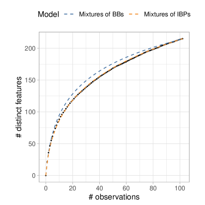
Figure 3: Left panel: the empirical accumulation curve (black dots) and the rarefaction curve of the models (blue and orange dashed lines). Right panel: the observed values of $K_{n,r}$ (black dots) compared with the expected curves $\mathds{E}(K_{n,r})$ (blue and orange dashed lines) for $r=1,\ldots,8$.

The extrapolation problem is addressed in Figure 4, where we report the expected values and the $95\%$ credible intervals for the total number of species that might be observed in $m$ additional plots, given the observed collection of $n$ plots, i.e., $K_{m}^{(n)}+k\mid\bm{Z}^{(n)}$, with $k=215$. The posterior point estimates are similar for the two selected prior variances, while the variability increases as the prior variance of $\gamma$ increases.

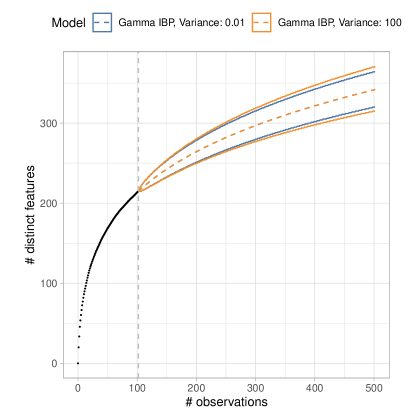
Figure 4: Expected values and the $95\%$ credible intervals for $K_{m}^{(n)}+k\mid\bm{Z}^{(n)}$, with $k=215$, for the gamma mixture of ibps. The extrapolation horizon is $m=1,\ldots,400$.

To provide a more quantitative answer to the extrapolation problem ecologists might be interested in, we report in Table 1 the expected values and the credible intervals for the number of new species that are going to be observed if a number $m$ of additional plots is examined, for some values of $m$. Both the choices for the prior variance of $\gamma$ in the gamma mixture of ibps lead to the same point-wise estimates: if ecologists are considering whether to analyze additional plots in the region, they should expect to find $6.50$ new species if they sample additional $m=10$ plots. Differences between the two gamma mixtures are visible for $m\in\{100,1000\}$ in terms of their credible intervals.

Table 1: Expected values $\mathds{E}(K_{m}^{(n)}\mid\bm{Z}^{(n)})$ and $95\%$ credible intervals (in brackets) for the statistic $K_{m}^{(n)}\mid\bm{Z}^{(n)}$, for $m\in\{1,10,100,1000\}$, for the vascular plants in Mazziotta et al. (2016a).

Gamma mixture of ibps $(n=102,k=215)$	$m=1$	$m=10$	$m=100$	$m=1000$
Prior variance $\text{Var}(\gamma)=0.01$	$0.673$ $[0,3]$	$6.50$ $[2,12]$	$50.1$ $[37,64]$	$204$ $[176,232]$
Prior variance $\text{Var}(\gamma)=100$	$0.673$ $[0,3]$	$6.50$ $[2,12]$	$50.1$ $[35,66]$	$204$ $[166,244]$

7.2 Trees in Barro Colorado Island

As a second illustration, we analyze the presence-absence dataset of tree species in $n=50$ plots of one hectare in Barro Colorado Island, for a total of $k=225$ observed species. The data are publicly available in the vegan package in R. In terms of richness estimation, exploring the taxon accumulation curve, reported in Figure S12 of the supplementary material, we may argue that it has not reached convergence yet, though the growth is rather slow. Overall, the species richness is expected to be larger than the $225$ observed species.

In order to select which model best fits the observed data, we perform the usual model-checking we introduced in Section 6.2. From the plots of Figure 5, we conclude that the mixtures of bbs can be considered correctly specified for such data, while the mixtures of ibps are not. Differently from the vascular plant data analyzed in the previous section, we thus claim that it is reasonable to assume that the species richness is finite. Hence we focus on the Poisson and negative binomial mixtures of bbs, as for the latter, we analyze two choices for the prior variance of $N$, i.e., $\operatornamewithlimits{Var}(N)=\mu_{0}\times c$, for $c\in\{10,1000\}$.

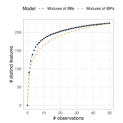
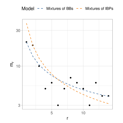
Figure 5: Left panel: the empirical accumulation curve (black dots) and the rarefaction curve of the models (blue and orange dashed lines). Right panel: the observed values of $K_{n,r}$ (black dots) compared with the expected curves $\mathds{E}(K_{n,r})$ (blue and orange dashed lines) for $r=1,\ldots,14$.

In such contexts, the species richness represents the most natural measure of biodiversity of the assemblage, therefore there is interest in estimating it. In the left panel of Figure 6, we report the posterior distribution of the species richness $N$, for the different mixtures of bbs. Specifically, the expected species richness is equal to $296.13$ for the Poisson mixture of bbs, with a credible interval equal to $[280,313]$. For both the negative binomial mixtures, we get an expected species richness of $296.17$, with credible intervals $[278,316]$.

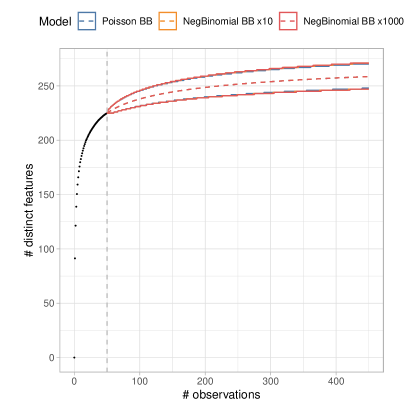
Figure 6: Left panel: posterior distributions of the species richness $N$ for different mixtures of bbs. Right panel: expected values and $95\%$ credible intervals for $K_{m}^{(n)}+k\mid\bm{Z}^{(n)}$, for different mixtures of bbs.

As far as the extrapolation problem is concerned, Figure 6 (right panel) reports the expected values and the $95\%$ credible intervals for the posteriors $K_{m}^{(n)}+k\mid\bm{Z}^{(n)}$, for $m=1,\ldots,400$, where $k=225$. It can be noted that the expected number of new features grows rather slowly with the size of the additional sample $m$; moreover, from Proposition 3, we remark that such a sequence $K_{m}^{(n)}+k\mid\bm{Z}^{(n)}$, $m=1,2,\ldots$, converges to the posterior distribution of the species richness $N$. As we have just discussed, all the mixtures of bbs that we have fitted provide an expected richness of around $296$.

We finally report the numerical values of expected values and the credible intervals for the number of new species that are going to be observed if a number $m$ of additional plots are sampled, for some values of $m$. All the mixtures of bbs fitted here provide the same point-wise estimates as well as the same credible intervals for $m\in\{1,10,100\}$: if ecologists are considering whether to analyze additional plots in the region, they should expect to find $0.41$ new species if they sample additional $m=1$ plots, $3.66$ new species for $m=10$ and $19.4$ new species for $m=100$. Moreover, the credible intervals are $[0,2]$ for $m=1$, $[0,8]$ for $m=10$ and $[11,29]$ for $m=100$. We can spot a difference among the models for $m=1000$: the expected number of new species is $41.8$, with credible intervals equal to $[30,55]$ for the Poisson mixture and $[29,56]$ for the negative binomial mixtures.

8 Discussion

In the present paper, we analyzed Gibbs-type feature models, namely those models exhibiting an efpf in product form (1). We argue that this class stands out among feature allocation models, similar to Gibbs-type priors, which play a fundamental role within species sampling models. We provided a comprehensive distribution theory for this class of models and a plethora of results in closed form. Additionally, we discussed two noteworthy examples: mixtures of ibps and mixtures of bbs. While the first class assumes an infinite number of features in the population, the latter can be adopted when the total number of features is supposed to be finite. We also proposed coherent methods for parameters’ elicitation and model selection. Finally, we have emphasized the importance of our findings in addressing ecological problems, such as estimating biodiversity and quantifying species richness. The code is available online at the link: https://github.com/LGhilotti/ProductFormFA.

Our contribution could pave the way for several future research directions. First, recall that we introduced a class of Gibbs-type feature models for exchangeable observations. However, in some applied problems, data are divided into different, though related, groups and the assumption of partial exchangeability would be more appropriate. Hence, an interesting direction for future research involves defining and investigating feature allocation models in the presence of multi-sample data. Although numerous models are available for partially exchangeable data within the species setting (Quintana et al., 2022), work is still ongoing in the framework of feature allocation models; see, e.g., Teh and Jordan (2010) for a few early examples. The availability of tractable classes of priors for grouped incidence data would enable the prediction for the number of shared species as well as the quantification of the so-called $\beta$-biodiversity, namely the heterogeneity among different ecological communities. Along these lines, the recent paper by Stolf and Dunson (2024) extends the ibp in defining a multivariate probit Indian buffet process.

Secondly, Gibbs-type are natural tools for modeling biodiversity when focusing on a single level of the Linnean taxonomy, such as family, genus or species. However, in modern sampling designs, each statistical unit often comprises a collection of $L$ different taxa, which are organized in a nested fashion; see, e.g., Zito et al. (2023b). As a crude exemplification, one might consider using a separate Gibbs-type feature model for each layer of the Linnean taxonomy. However, this approach would overlook the rich and informative nested structure of the data. Bayesian nonparametric models for such data are underdeveloped even for species sampling models, and there is ample room for new ideas and theoretical developments.

Thirdly, a potentially impactful ramification of our results pertains to the usage of Gibbs-type feature models as a building block of more complex hierarchical models, i.e., when employed as a latent component. We refer to Griffiths and Ghahramani (2011) for a general discussion. Among the potential applications of Gibbs-type feature models, it is worth mentioning their role in Bayesian factor analysis, in which $N$, in our notation, would represent the number of factors. The ibp has been successfully used in this context to incorporate sparsity for instance to model gene expression data (Knowles and Ghahramani, 2011). A further example is given by Ayed and Caron (2021), who explored suitable extensions of the ibp to discover latent communities in network data. Our paper provides several alternatives to the ibp for Bayesian factor models and related applications. It is also worth mentioning that the mixtures of bbs, unlike the traditional ibp or the bb, enable the incorporation of prior opinions on the number of latent factors in Bayesian modeling. Work on these problems is deemed to be future research.

Supplementary material for:
“Bayesian analysis of product feature allocation models”

Organization of the supplementary material

The supplementary material is organized as follows. In Section S1, we prove all the general results of Section 3, valid for any Gibbs-type feature model. In addition, in Section S1.4 we provide general distributional results for the statistic $K_{n,r}$, denoting the number of features appearing exactly $r$ times across $n$ individuals. Section S1.5 specializes the general distribution theory for $K_{n,r}$ under the Poisson and negative binomial mixtures of bbs and the gamma mixture of ibps. Section S2 (resp. Section S3) contains all the proofs and details of Section 4 (resp. Section 5). Our simulation studies are reported in Section S4. Finally, Section S5 includes additional plots referring to the ecological applications presented in the main paper; moreover, in Section S5.2, we also propose a fully Bayesian approach for parameters’ elicitation, alternative to the empirical Bayes one described in Section 6.1. We apply such a fully Bayesian approach to the two real data scenarios of Section 7 in comparison with the inference obtained via the empirical Bayes procedure.

S1 Proofs of Section 3 and additional results

S1.1 Proof of Theorem 1

In order to determine the predictive distribution, we have to pay attention to the ordering of the new features. More precisely, if $K_{n}=k$, there are $\binom{k+y}{k}$ possible ways to order the new $Y_{n+1}=y$ observed features with respect to the first $K_{n}$ ordered features. By taking into account this combinatorial coefficient, the predictive law equals

$$p_{n}(y,a_{1},\ldots,a_{k})=\frac{\binom{k+y}{k}\pi_{n+1}(m_{1}+a_{1},\ldots,m_{k}+a_{k},1,\ldots,1)}{\pi_{n}(m_{1},\ldots,m_{k})}$$

where the number $1$ at the numerator is repeated $y$ times. The numerator corresponds to the probability of the feature allocation induced by the observed sample $\bm{Z}^{(n)}$ and $Z_{n+1}$, by considering all the possible orders of the $y$ newly observed features. Besides, the denominator is the probability distribution of the feature allocation induced by the sample $\bm{Z}^{(n)}$. By substituting the specific expression of the efpf in product form (1), we obtain

$$p_{n}(y,a_{1},\ldots,a_{k})=\binom{k+y}{k}\frac{V_{n+1,k+y}}{V_{n,k}}(\theta+\alpha)_{n}^{y}\cdot\prod_{\ell=1}^{k}\frac{(1-\alpha)_{m_{\ell}+a_{\ell}-1}}{(1-\alpha)_{m_{\ell}-1}}\frac{(\theta+\alpha)_{n+1-m_{\ell}-a_{\ell}}}{(\theta+\alpha)_{n-m_{\ell}}}.$$

By observing that

$$\frac{(1-\alpha)_{m_{\ell}+a_{\ell}-1}}{(1-\alpha)_{m_{\ell}-1}}=(m_{\ell}-\alpha)^{a_{\ell}},\quad\frac{(\theta+\alpha)_{n+1-m_{\ell}-a_{\ell}}}{(\theta+\alpha)_{n-m_{\ell}}}=(\theta+\alpha+n-m_{\ell})^{1-a_{\ell}},$$

we get the following expression:

$$\begin{split}p_{n}(y,a_{1},\ldots,a_{k})&=\binom{k+y}{k}\frac{V_{n+1,k+y}}{V_{n,k}}\{(\theta+\alpha)_{n}\}^{y}(\theta+n)^{k}\prod_{\ell=1}^{k}\left(\frac{m_{\ell}-\alpha}{\theta+n}\right)^{a_{\ell}}\cdot\left(1-\frac{m_{\ell}-\alpha}{\theta+n}\right)^{1-a_{\ell}}\\ &=\binom{k+y}{k}\frac{V_{n+1,k+y}}{V_{n,k}}\{(\theta+\alpha)_{n}\}^{y}(\theta+n)^{k}\prod_{\ell=1}^{k}\mathscr{B}\left(a_{\ell};\frac{m_{\ell}-\alpha}{\theta+n}\right)\end{split}$$

and the thesis follows.

S1.2 Proof of Corollary 1

The corollary easily follows from Theorem 1. Indeed, the sample coverage equals

$$\begin{split}\mathds{P}(Y_{n+1}=0\mid\bm{Z}^{(n)})&=\sum_{(a_{1},\ldots,a_{k})\in\{0,1\}^{k}}p_{n}(0,a_{1},\ldots,a_{k})=\frac{V_{n+1,k}}{V_{n,k}}(\theta+n)^{k}\prod_{\ell=1}^{k}\sum_{a_{\ell}=0}^{1}\mathscr{B}\left(a_{\ell};\frac{m_{\ell}-\alpha}{\theta+n}\right)\\ &=\frac{V_{n+1,k}}{V_{n,k}}(\theta+n)^{k}\end{split}$$

where we have marginalized out the probability of observing old features from the predictive distribution.

S1.3 Proof of Theorem 2

We start by proving the following lemma, which provides the probability distribution of $K_{n}$ for any exchangeable feature allocation model admitting an efpf.

Lemma S1.

For any feature allocation model admitting an efpf, the probability distribution of $K_{n}$ is

$$\mathds{P}(K_{n}=k)=\sum_{\begin{subarray}{c}m_{\ell}\in\{1,\ldots,n\}\\ \ell=1,\ldots,k\end{subarray}}\pi_{n}(m_{1},\ldots,m_{k})\binom{n}{m_{1}}\cdots\binom{n}{m_{k}}.$$

Proof.

The event $\{K_{n}=k\}$ corresponds to the union of all feature allocations of the type $F_{n}=(B_{n,1},\ldots,B_{n,k})$, where $m_{\ell}=|B_{n,\ell}|$ takes any value in the set $\{1,\ldots,n\}$, for any $\ell=1,\ldots,k$. For a specific configuration of $(m_{1},\ldots,m_{k})$, there are several feature allocations $F_{n}$ such that $m_{\ell}=|B_{n,\ell}|$, as $\ell=1,\ldots,k$. Indeed, there are $\binom{n}{m_{1}}$ different ways to choose the indexes in the set $[n]$ to define $B_{n,1}$, similarly there are $\binom{n}{m_{2}}$ different ways to choose the set $B_{n,2}$, etc.. Hence, the probability of observing all feature allocations having predetermined block sizes $(m_{1},\ldots,m_{k})$ equals $\pi_{n}(m_{1},\ldots,m_{k})\binom{n}{m_{1}}\cdots\binom{n}{m_{k}}$. As a consequence, the probability $\mathds{P}(K_{n}=k)$ can be obtained by summing over all the possible configurations of the vector $(m_{1},\ldots,m_{k})\in\{1,\ldots,n\}^{k}$. ∎

We now exploit Lemma S1 to find the probability distribution of $K_{n}$ for any Gibbs-type feature allocation model:

$$\mathds{P}(K_{n}=k) =\sum_{\begin{subarray}{c}m_{\ell}\in\{1,\ldots,n\}\\ \ell=1,\ldots,k\end{subarray}}V_{n,k}\prod_{\ell=1}^{k}(1-\alpha)_{m_{\ell}-1}(\theta+\alpha)_{n-m_{\ell}}\binom{n}{m_{\ell}}$$ (S1)

$$=V_{n,k}\prod_{\ell=1}^{k}\sum_{m_{\ell}=1}^{n}\binom{n}{m_{\ell}}(1-\alpha)_{m_{\ell}-1}(\theta+\alpha)_{n-m_{\ell}}$$

$$=V_{n,k}\left[\sum_{i=1}^{n}\binom{n}{i}(1-\alpha)_{i-1}(\theta+\alpha)_{n-i}\right]^{k}.$$

We now consider the case $\alpha<0$ and $\alpha\in[0,1)$ separately.

Case $\bm{\alpha<0}$. For these values of $\alpha$, the last sum in (S1) can be expressed as

$$\sum_{i=1}^{n}\binom{n}{i}(1-\alpha)_{i-1}(\theta+\alpha)_{n-i}=\frac{\Gamma(-\alpha)}{\Gamma(1-\alpha)}\sum_{i=0}^{n}\binom{n}{i}(-\alpha)_{i}(\theta+\alpha)_{n-i}+\frac{(\theta+\alpha)_{n}}{\alpha}.$$

Thanks to the Chu-Vandermonde identity, we obtain

$$\frac{\Gamma(-\alpha)}{\Gamma(1-\alpha)}\sum_{i=0}^{n}\binom{n}{i}(-\alpha)_{i}(\theta+\alpha)_{n-i}+\frac{(\theta+\alpha)_{n}}{\alpha}=-\frac{(\theta)_{n}}{\alpha}+\frac{(\theta+\alpha)_{n}}{\alpha}$$

and the thesis follows for $\alpha<0$.

Case $\bm{\alpha\in[0,1)}$. For positive values of $\alpha$, the sum in (S1) can be expressed as

$$\begin{split}\sum_{i=1}^{n}\binom{n}{i}(1-\alpha)_{i-1}&(\theta+\alpha)_{n-i}=\sum_{i=1}^{n}\binom{n}{i}\frac{\Gamma(i-\alpha)}{\Gamma(1-\alpha)}\frac{\Gamma(\theta+\alpha+n-i)}{\Gamma(\theta+\alpha)}\cdot\frac{\Gamma(\theta+n)}{\Gamma(\theta+n)}\\ &=\frac{\Gamma(\theta+n)}{\Gamma(1-\alpha)\Gamma(\theta+\alpha)}\sum_{i=1}^{n}\binom{n}{i}B(i-\alpha,\theta+\alpha+n-i),\end{split}$$

where $B(a,b)$ denotes the Euler’s beta function evaluated at $a,b>0$. Thanks to the integral representation of the beta function, one obtains:

$$\begin{split}\sum_{i=1}^{n}\binom{n}{i}(1-\alpha)_{i-1}&(\theta+\alpha)_{n-i}=\frac{\Gamma(\theta+n)}{\Gamma(1-\alpha)\Gamma(\theta+\alpha)}\sum_{i=1}^{n}\binom{n}{i}\int_{0}^{1}x^{i-\alpha-1}(1-x)^{\theta+\alpha+n-i-1}{\rm d}x\\ &=\frac{\Gamma(\theta+n)}{\Gamma(1-\alpha)\Gamma(\theta+\alpha)}\int_{0}^{1}x^{-\alpha-1}(1-x)^{\theta+\alpha+n-1}\sum_{i=1}^{n}\binom{n}{i}\left(\frac{x}{1-x}\right)^{i}{\rm d}x\\ &=\frac{\Gamma(\theta+n)}{\Gamma(1-\alpha)\Gamma(\theta+\alpha)}\int_{0}^{1}x^{-\alpha-1}(1-x)^{\theta+\alpha+n-1}\left[\left(\frac{x}{1-x}+1\right)^{n}-1\right]{\rm d}x\\ &=\frac{\Gamma(\theta+n)}{\Gamma(1-\alpha)\Gamma(\theta+\alpha)}\int_{0}^{1}x^{-\alpha-1}(1-x)^{\theta+\alpha+n-1}\left[\left(\frac{1}{1-x}\right)^{n}-1\right]{\rm d}x\\ &=\frac{\Gamma(\theta+n)}{\Gamma(1-\alpha)\Gamma(\theta+\alpha)}\int_{0}^{1}x^{-\alpha-1}(1-x)^{\theta+\alpha-1}\left[1-(1-x)^{n}\right]{\rm d}x.\end{split}$$

By virtue of the following equality

$$1-(1-x)^{n}=x\sum_{i=0}^{n-1}(1-x)^{i},$$

we obtain

$$\frac{\Gamma(\theta+n)}{\Gamma(1-\alpha)\Gamma(\theta+\alpha)} \int_{0}^{1}x^{-\alpha-1}(1-x)^{\theta+\alpha-1}\left[1-(1-x)^{n}\right]{\rm d}x$$

$$=\frac{\Gamma(\theta+n)}{\Gamma(1-\alpha)\Gamma(\theta+\alpha)}\int_{0}^{1}x^{-\alpha+1-1}(1-x)^{\theta+\alpha-1}\sum_{i=0}^{n-1}(1-x)^{i}{\rm d}x$$

$$=\frac{\Gamma(\theta+n)}{\Gamma(1-\alpha)\Gamma(\theta+\alpha)}\sum_{i=0}^{n-1}\int_{0}^{1}x^{-\alpha+1-1}(1-x)^{\theta+\alpha+i-1}{\rm d}x$$

$$=\frac{\Gamma(\theta+n)}{\Gamma(1-\alpha)\Gamma(\theta+\alpha)}\sum_{i=0}^{n-1}\frac{\Gamma(i+\theta+\alpha)\Gamma(1-\alpha)}{\Gamma(i+\theta+1)}$$

$$=\frac{\Gamma(\theta+n)}{\Gamma(1-\alpha)\Gamma(\theta+\alpha)}\sum_{i=1}^{n}\frac{\Gamma(i+\theta+\alpha-1)\Gamma(1-\alpha)}{\Gamma(i+\theta)}$$

$$=\frac{\Gamma(\theta+n)}{\Gamma(\theta+1)}\sum_{i=1}^{n}\frac{(\theta+\alpha)_{i-1}}{(\theta+1)_{i-1}}=(\theta+1)_{n-1}\sum_{i=1}^{n}\frac{(\theta+\alpha)_{i-1}}{(\theta+1)_{i-1}}$$

and the thesis follows by substituting the previous expression in (S1).

S1.4 Distributional results for the number of $r$-shared features $K_{n,r}$

Here we provide distributional results for the statistic $K_{n,r}$, where $r\in\{1,\ldots,n\}$, denoting the number of features appearing exactly $r$ times among $n$ individuals. We start by proving the following lemma, which provides the probability distribution of $K_{n,r}$ for any feature allocation model admitting an efpf.

Lemma S2.

For any feature allocation model admitting an efpf, the distribution of $K_{n,r}$ equals

$$\begin{split}&\mathds{P}(K_{n,r}=y)\\ &\qquad=\binom{n}{r}^{y}\Bigg{\{}\pi_{n}(r,\ldots,r)+\sum_{k=y+1}^{\infty}\binom{k}{y}\sum_{\begin{subarray}{c}m_{\ell}\in\{1,\ldots,n\}\\ m_{\ell}\neq r\\ \ell=1,\ldots,k-y\end{subarray}}\pi_{n}(r,\ldots,r,m_{1},\ldots,m_{k-y})\prod_{\ell=1}^{k-y}\binom{n}{m_{\ell}}\Bigg{\}}\end{split}$$ (S2)

where $(r,\ldots,r)$ in the previous expression is a vector of length $y$.

Proof.

The event $\{K_{n,r}=y\}$ corresponds to all random ordered feature allocations of the type $F_{n}=(B_{n,1},\ldots,B_{n,k})$, where $k\geq y$ and there are exactly $y$ sets out of the $B_{n,\ell}$’s with cardinality $r$.
Consider $k>y$, and suppose that the first $y$ sets are those with cardinality $r$, i.e., $|B_{n,\ell}|=r$, for all ${\ell}=1,\ldots,y$, and that the remaining sets $B_{n,y+\ell}$, as $\ell=1,\ldots,k-y$, have cardinalities $m_{\ell}\in\{1,\ldots,n\}$, where $m_{\ell}\neq r$. There are $\binom{n}{r}$ different ways to choose the indexes in $[n]$ to construct each of the first $y$ blocks $B_{n,\ell}$, as $\ell=1,\ldots,y$. Analogously, there are $\binom{n}{m_{\ell}}$ different ways to define $B_{n,y+\ell}$, as $\ell=1,\ldots,k-y$. Thus, the probability of observing all feature allocations having the first $y(<k)$ blocks with cardinality $r$ equals

$$\pi_{n}(r,\ldots,r,m_{1},\ldots,m_{k-y})\binom{n}{r}^{y}\binom{n}{m_{1}}\cdots\binom{n}{m_{k-y}}.$$

The previous probability refers to all the feature allocations where the first $y$ blocks have cardinality $r$, it is apparent that we have to multiply by the factor $\binom{k}{y}$ to take into account all the possible rearrangements of the $y$ blocks with cardinality $r$. When $k=y$, the probability that all the blocks of the feature allocation have cardinality $r$ equals $\pi_{n}(r,\ldots,r)\binom{n}{r}^{y}$, where $(r,\ldots,r)$ is a vector of length $y$. The expression of $\mathds{P}(K_{n,r}=y)$ can be obtained by summing the previous probabilities when $k\geq y$:

$$\mathds{P}(K_{n,r}=y) =\pi_{n}(r,\ldots,r)\binom{n}{r}^{y}+$$

$$\quad\sum_{k=y+1}^{\infty}\sum_{\begin{subarray}{c}m_{\ell}\in\{1,\ldots,n\}\\ m_{\ell}\neq r\\ \ell=1,\ldots,k-y\end{subarray}}\binom{k}{y}\pi_{n}(r,\ldots,r,m_{1},\ldots,m_{k-y})\binom{n}{r}^{y}\prod_{\ell=1}^{k-y}\binom{n}{m_{\ell}}$$

and the thesis now follows. ∎

We now state our main result of the section by specializing the previous lemma to the class of Gibbs-type feature allocation models.

Proposition S1 (Number of $r$-shared features $K_{n,r}$).

Suppose the efpf is in product form (1). Then, for any $k\geq 0$,

$$\mathds{P}(K_{n,r}=k)=\left\{\binom{n}{r}(1-\alpha)_{r-1}(\theta+\alpha)_{n-r}\right\}^{k}\sum_{j=0}^{\infty}\binom{j+k}{k}V_{n,j+k}\{t_{n,r}(\theta,\alpha)\}^{k},$$

where, if $\alpha<0$,

$$t_{n,r}(\theta,\alpha)=-\frac{(\theta)_{n}}{\alpha}+\frac{(\theta+\alpha)_{n}}{\alpha}-\binom{n}{r}(1-\alpha)_{r-1}(\theta+\alpha)_{n-r},$$

whereas, if $\alpha\in[0,1)$,

$$t_{n,r}(\theta,\alpha)=(\theta+1)_{n-1}\>g_{n}(\theta,\alpha)-\binom{n}{r}(1-\alpha)_{r-1}(\theta+\alpha)_{n-r}.$$

Proof.

We exploit Lemma S2 to evaluate $\mathds{P}(K_{n,r}=y)$ for the Gibbs-type feature allocation models. A plain application of Equation (S2) leads to

$$\mathds{P}(K_{n,r}=y) =\left[\binom{n}{r}(1-\alpha)_{r-1}(\theta+\alpha)_{n-r}\right]^{y}$$

$$\qquad\times\Bigg{\{}V_{n,y}+\sum_{z=1}^{\infty}\binom{z+y}{y}V_{n,z+y}\sum_{\begin{subarray}{c}m_{\ell}\in\{1,\ldots,n\}\\ m_{\ell}\neq r\\ \ell=1,\ldots,k-y\end{subarray}}\prod_{\ell=1}^{z}\binom{n}{m_{\ell}}(1-\alpha)_{m_{\ell}-1}(\theta+\alpha)_{n-m_{\ell}}\Bigg{\}}$$

$$=\left[\binom{n}{r}(1-\alpha)_{r-1}(\theta+\alpha)_{n-r}\right]^{y}\times$$

$$\qquad\times\sum_{z=0}^{\infty}\binom{z+y}{y}V_{n,z+y}\Bigg{[}\sum_{\begin{subarray}{c}i\in\{1,\ldots,n\}\\ i\neq r\end{subarray}}\binom{n}{i}(1-\alpha)_{i-1}(\theta+\alpha)_{n-i}\Bigg{]}^{z}$$

$$=\left[\binom{n}{r}(1-\alpha)_{r-1}(\theta+\alpha)_{n-r}\right]^{y}\times$$

$$\qquad\times\sum_{z=0}^{\infty}\binom{z+y}{y}V_{n,z+y}\Bigg{[}\sum_{i=1}^{n}\binom{n}{i}(1-\alpha)_{i-1}(\theta+\alpha)_{n-i}-\binom{n}{r}(1-\alpha)_{r-1}(\theta+\alpha)_{n-r}\Bigg{]}^{z}.$$

We can now apply a similar strategy as in the proof of Theorem 2 to get the expressions for the case $\alpha<0$ and $\alpha\in[0,1)$. ∎

S1.5 Additional specialized results for novel models

The general expression for the number of $r$-shared features $K_{n,r}$ presented in Proposition S1 can be specialized in the case of gamma mixture of ibps and Poisson and negative binomial mixtures of bbs, leading to standard and well-known probability distributions. In the following proposition, we report the specialized results for the mixtures of bbs.

Proposition S2.

Suppose the efpf is in product form (1) with $\alpha<0$ and let $b_{n,r}(\theta,\alpha):=-\alpha\binom{n}{r}(1-\alpha)_{r-1}(\theta+\alpha)_{n-r}/(\theta)_{n}$. If $N$ is fixed, corresponding to the bb model (3), then

$$K_{n,r}\mid N\sim\textup{Binomial}\left(N,b_{n,r}\right).$$

If instead $N\sim\textup{Poisson}(\lambda)$, corresponding to model (17), then

$$K_{n,r}\sim\textup{Poisson}\left(\lambda\cdot b_{n,r}\right).$$

Finally, if $N\sim\textup{NegBinomial}(n_{0},\mu_{0})$, corresponding to model (18), then

$$K_{n,r}\sim\textup{NegBinomial}\left(n_{0},\mu_{0}\cdot b_{n,r}\right).$$

For the gamma mixture of ibps, the prior distribution of $K_{n,r}$ is described in the next proposition.

Proposition S3.

Suppose the efpf is in product form (1) with $\alpha\in[0,1)$ and $d_{n,r}:=\binom{n}{r}(1-\alpha)_{r-1}(\theta+\alpha)_{n-r}\Gamma(\theta+1)/\Gamma(\theta+n)$. If $\gamma$ is fixed, corresponding to the ibp model (2), then

$$K_{n,r}\mid\gamma\sim\textup{Poisson}\left(\gamma\cdot d_{n,r}\right).$$

If instead $\gamma\sim\textup{Gamma}(a,b)$, then

$$K_{n,r}\sim\textup{NegBinomial}\left(a,a/b\cdot d_{n,r}\right).$$

S1.6 Proof of Theorem 3

We start by proving the following lemma, which provides the probability distribution of $K_{m}^{(n)}\mid\bm{Z}^{(n)}$ for any feature allocation model admitting an efpf.

Lemma S3.

For any feature allocation model admitting an efpf, the distribution of $K_{m}^{(n)}\mid\bm{Z}^{(n)}$ equals

$$\mathds{P}(K_{m}^{(n)}=y\mid\bm{Z}^{(n)})=\binom{k+y}{k}\frac{1}{\pi_{n}(m_{1},\ldots,m_{k})}$$

$$\qquad\qquad\times\sum_{\begin{subarray}{c}r_{t}\in\{1,\ldots,m\}\\ t=1,\ldots,y\end{subarray}}\sum_{\begin{subarray}{c}c_{\ell}\in\{0,\ldots,m\}\\ \ell=1,\ldots,k\end{subarray}}\pi_{n+m}(m_{1}+c_{1},\ldots,m_{k}+c_{k},r_{1},\ldots,r_{y})\prod_{r=1}^{y}\binom{m}{r_{t}}\prod_{\ell=1}^{k}\binom{m}{c_{\ell}}.$$

Proof.

We denote by $F_{n}=(B_{n,1},\ldots,B_{n,K_{n}})$ the random ordered feature allocation corresponding to the random sample $\bm{Z}^{(n)}$, and by $f_{n}$ the observed value of $F_{n}$. Thanks to the correspondence between $\bm{Z}^{(n)}$ and $F_{n}$, as explained by Broderick et al. (2013), we have

$$\mathds{P}(K_{m}^{(n)}=y\mid\bm{Z}^{(n)})=\frac{\mathds{P}(K_{m}^{(n)}=y,F_{n}=f_{n})}{\mathds{P}(F_{n}=f_{n})},$$ (S3)

where we observe that $\mathds{P}(F_{n}=f_{n})=\pi_{n}(m_{1},\ldots,m_{k})$. Denote by $(B_{m+n,1},\ldots,B_{m+n,k})$ the random ordered feature allocation which refers to the old features, and by $(B_{m+n,k+1},\ldots,B_{m+n,k+y})$ the random ordered feature allocation corresponding to the $y$ new features. In order to evaluate the probability at the numerator in (S3), we need to evaluate the probability that the aforementioned random ordered feature allocations satisfy:

• $(B_{m+n,1},\ldots,B_{m+n,k})$ is consistent with the initial $F_{n}$, in the sense that each set $B_{m+n,\ell}$ contains the $m_{\ell}$ indexes of the corresponding $B_{n,\ell}$, as $\ell=1,\ldots,k$;

• each set in $(B_{m+n,1},\ldots,B_{m+n,k})$ contains $c_{\ell}$ indexes from $\{n+1,\ldots,n+m\}$, for all the possible choices of $c_{\ell}\in\{0,\ldots,m\}$, as $\ell=1,\ldots,k$;

• the sets $B_{m+n,k+1},\ldots,B_{m+n,k+y}$, corresponding to the new features, contain $r_{t}$ indexes out of the set $\{n+1,\ldots,n+m\}$, for all the possible choices of $r_{t}\in\{1,\ldots,m\}$, as $t=1,\ldots,y$.

We note that $B_{m+n,\ell}$ can be chosen in $\binom{m}{c_{\ell}}$ different ways, as $\ell=1,\ldots,k$, because this is the number of possible ways to select $c_{\ell}$ indexes among $\{n+1,\ldots,n+m\}$ of the subjects displaying feature $\ell$. Besides, $B_{m+n,k+t}$ can be chosen in $\binom{m}{r_{t}}$ different ways, as $t=1,\ldots,y$. The probability of observing random ordered feature allocations satisfying (i)–(iii) equals

$$\pi_{n+m}(m_{1}+c_{1},\ldots,m_{k}+c_{k},r_{1},\ldots,r_{y})\prod_{t=1}^{y}\binom{m}{r_{t}}\prod_{\ell=1}^{k}\binom{m}{c_{\ell}}.$$

We finally observe that there are $\binom{k+y}{y}$ possible ways for ordering the $y$ new features among the $k$ old features, as a consequence one has:

$$\mathds{P}(K_{m}^{(n)}=y\mid\bm{Z}^{(n)})=\frac{1}{\pi_{n}(m_{1},\ldots,m_{k})}$$

$$\qquad\qquad\times\sum_{\begin{subarray}{c}r_{t}\in\{1,\ldots,m\}\\ t=1,\ldots,y\end{subarray}}\sum_{\begin{subarray}{c}c_{\ell}\in\{0,\ldots,m\}\\ \ell=1,\ldots,k\end{subarray}}\pi_{n+m}(m_{1}+c_{1},\ldots,m_{k}+c_{k},r_{1},\ldots,r_{y})\prod_{r=1}^{y}\binom{m}{r_{t}}\prod_{\ell=1}^{k}\binom{m}{c_{\ell}}\binom{k+y}{k}$$

and the thesis follows. ∎

We now concentrate on the posterior probability distribution of $K_{m}^{(n)}$ in Gibbs-type feature allocation models. By virtue of Lemma S3, one has:

$$\mathds{P}(K_{m}^{(n)}=y\mid\bm{Z}^{(n)}) =\binom{k+y}{k}\frac{V_{n+m,k+y}}{\pi_{n}(m_{1},\ldots,m_{k})}\sum_{\begin{subarray}{c}r_{t}\in\{1,\ldots,m\}\\ t=1,\ldots,y\end{subarray}}\prod_{t=1}^{y}\binom{m}{r_{t}}(1-\alpha)_{r_{t}-1}(\theta+\alpha)_{n+m-r_{t}}$$ (S4)

$$\qquad\qquad\times\sum_{\begin{subarray}{c}c_{\ell}\in\{0,\ldots,m\}\\ \ell=1,\ldots,k\end{subarray}}\prod_{\ell=1}^{k}\binom{m}{c_{\ell}}(1-\alpha)_{m_{\ell}+c_{\ell}-1}(\theta+\alpha)_{n+m-m_{\ell}-c_{\ell}}.$$

First, consider the following sum

$$\sum_{\begin{subarray}{c}c_{\ell}\in\{0,\ldots,m\}\\ \ell=1,\ldots,k\end{subarray}}\prod_{\ell=1}^{k}\binom{m}{c_{\ell}}(1-\alpha)_{m_{\ell}+c_{\ell}-1}(\theta+\alpha)_{n+m-m_{\ell}-c_{\ell}}=\prod_{\ell=1}^{k}\sum_{c_{\ell}=0}^{m}\binom{m}{c_{\ell}}(1-\alpha)_{m_{\ell}+c_{\ell}-1}(\theta+\alpha)_{n+m-m_{\ell}-c_{\ell}},$$

by observing that

$$(1-\alpha)_{m_{\ell}+c_{\ell}-1}=(1-\alpha)_{m_{\ell}-1}(m_{\ell}-\alpha)_{c_{\ell}}$$

and

$$(\theta+\alpha)_{n+m-m_{\ell}-c_{\ell}}=(\theta+\alpha)_{n-m_{\ell}}(\theta+\alpha+n-m_{\ell})_{m-c_{\ell}},$$

the Chu-Vandermonde identity implies

$$\prod_{\ell=1}^{k}\sum_{c_{\ell}=0}^{m}\binom{m}{c_{\ell}}(1-\alpha)_{m_{\ell}+c_{\ell}-1}(\theta+\alpha)_{n+m-m_{\ell}-c_{\ell}}=\prod_{\ell=1}^{k}\Bigg{[}(1-\alpha)_{m_{\ell}-1}(\theta+\alpha)_{n-m_{\ell}}(\theta+n)_{m}\Bigg{]}.$$

By exploiting the previous identity and the expression of the efpf (1), the probability of interest (S4) boils down to

$$\mathds{P}(K_{m}^{(n)}=y\mid\bm{Z}^{(n)})=\binom{k+y}{k}\frac{V_{n+m,k+y}}{V_{n,k}}(\theta+n)_{m}^{k}\left[\sum_{i=1}^{m}\binom{m}{i}(1-\alpha)_{i-1}(\theta+\alpha)_{n+m-i}\right]^{y}.$$ (S5)

We now consider separately the two cases $\alpha<0$ and $\alpha\in[0,1)$.
Case $\bm{\alpha<0}$. For such values of $\alpha$, we observe that

$$(1-\alpha)_{i-1}=-\frac{1}{\alpha}(-\alpha)_{i}\quad\text{and}\quad(\theta+\alpha)_{n+m-i}=(\theta+\alpha)_{n}(\theta+\alpha+n)_{m-i},$$

and, thanks to the Chu-Vandermonde identity, one has

$$\sum_{i=1}^{m}\binom{m}{i}(1-\alpha)_{i-1}(\theta+\alpha)_{n+m-i}=-\frac{1}{\alpha}(\theta+\alpha)_{n}\left[(\theta+n)_{m}-(\theta+\alpha+n)_{m}\right].$$

The result for $\alpha<0$ follows by substituting the previous expression in (S5).

Case $\bm{\alpha\in[0,1)}$. As for $\alpha\in[0,1)$, the sum appearing in (S5) can be rewritten as follows:

$$\sum_{i=1}^{m}\binom{m}{i}(1-\alpha)_{i-1} (\theta+\alpha)_{n+m-i}=\sum_{i=1}^{m}\binom{m}{i}\frac{\Gamma(i-\alpha)}{\Gamma(1-\alpha)}\frac{\Gamma(\theta+\alpha+m+n-i)}{\Gamma(\theta+\alpha)}\cdot\frac{\Gamma(\theta+m+n)}{\Gamma(\theta+m+n)}$$

$$=\frac{\Gamma(\theta+m+n)}{\Gamma(1-\alpha)\Gamma(\theta+\alpha)}\sum_{i=1}^{m}\binom{m}{i}B(i-\alpha,\theta+\alpha+m+n-i).$$

We can now use the integral representation of the beta function to get

$$\sum_{i=1}^{m}\binom{m}{i}(1-\alpha)_{i-1} (\theta+\alpha)_{n+m-i}=\frac{\Gamma(\theta+m+n)}{\Gamma(1-\alpha)\Gamma(\theta+\alpha)}\sum_{i=1}^{m}\binom{m}{i}\int_{0}^{1}x^{i-\alpha-1}(1-x)^{\theta+\alpha+m+n-i-1}{\rm d}x$$

$$=\frac{\Gamma(\theta+m+n)}{\Gamma(1-\alpha)\Gamma(\theta+\alpha)}\int_{0}^{1}x^{-\alpha-1}(1-x)^{\theta+\alpha+m+n-1}\sum_{i=1}^{m}\binom{m}{i}\left(\frac{x}{1-x}\right)^{i}{\rm d}x$$

$$=\frac{\Gamma(\theta+m+n)}{\Gamma(1-\alpha)\Gamma(\theta+\alpha)}\int_{0}^{1}x^{-\alpha-1}(1-x)^{\theta+\alpha+m+n-1}\left[\left(\frac{x}{1-x}+1\right)^{m}-1\right]{\rm d}x$$

$$=\frac{\Gamma(\theta+m+n)}{\Gamma(1-\alpha)\Gamma(\theta+\alpha)}\int_{0}^{1}x^{-\alpha-1}(1-x)^{\theta+\alpha+n-1}\left[1-(1-x)^{m}\right]{\rm d}x.$$

By virtue of the simple identity

$$1-(1-x)^{m}=x\sum_{i=0}^{m-1}(1-x)^{i},$$

the previous expression becomes

$$\sum_{i=1}^{m}\binom{m}{i}(1-\alpha)_{i-1} (\theta+\alpha)_{n+m-i}$$

$$=\frac{\Gamma(\theta+m+n)}{\Gamma(1-\alpha)\Gamma(\theta+\alpha)}\int_{0}^{1}x^{-\alpha+1-1}(1-x)^{\theta+\alpha+n-1}\sum_{i=0}^{m-1}(1-x)^{i}{\rm d}x$$

$$=\frac{\Gamma(\theta+m+n)}{\Gamma(1-\alpha)\Gamma(\theta+\alpha)}\sum_{i=0}^{m-1}\int_{0}^{1}x^{-\alpha+1-1}(1-x)^{\theta+\alpha+n+i-1}{\rm d}x$$

$$=\frac{\Gamma(\theta+m+n)}{\Gamma(1-\alpha)\Gamma(\theta+\alpha)}\sum_{i=0}^{m-1}\frac{\Gamma(i+\theta+\alpha+n)\Gamma(1-\alpha)}{\Gamma(i+\theta+n+1)}$$

$$=\frac{\Gamma(\theta+m+n)}{\Gamma(1-\alpha)\Gamma(\theta+\alpha)}\sum_{i=1}^{m}\frac{\Gamma(i+\theta+\alpha+n-1)\Gamma(1-\alpha)}{\Gamma(i+\theta+n)}$$

$$=\frac{\Gamma(\theta+m+n)}{\Gamma(\theta+1)}\sum_{i=1}^{m}\frac{(\theta+\alpha)_{n+i-1}}{(\theta+1)_{n+i-1}}=(\theta+1)_{m+n-1}\sum_{i=1}^{m}\frac{(\theta+\alpha)_{n+i-1}}{(\theta+1)_{n+i-1}}$$

$$=(\theta+1)_{n-1}(\theta+n)_{m}\sum_{i=1}^{m}\frac{(\theta+\alpha)_{n+i-1}}{(\theta+1)_{n+i-1}}$$

and the thesis for $\alpha\in[0,1)$ follows by substituting this expression in (S5).

S1.7 Proof of Proposition 2

The asymptotic behavior of $K_{n}$ follows by specializing the asymptotic distribution of $K_{m}^{(n)}$, determined in Proposition 3, when $n=0$ and $m$ is replaced with $n$. One may also prove this result by working along the same lines as in the proof of Proposition 3.

S1.8 Proof of Proposition 3

We prove the theorem for $\alpha<0$, $\alpha=0$ and $\alpha\in(0,1)$ separately.
Case $\alpha<0$. This choice corresponds to a mixture over $N$ of a bb model. We first observe that, in the case of a bb model with parameter $N$, the posterior distribution of the number of hitherto unseen features $K_{m}^{(n)}\mid\bm{Z}^{(n)},N$ has a binomial distribution given by

$$K_{m}^{(n)}\mid\bm{Z}^{(n)},N\sim\textup{Binomial}\Big{(}N-k,1-\frac{(\theta+\alpha+n)_{m}}{(\theta+n)_{m}}\Big{)}.$$

This result is a simple consequence of Theorem 3 that can be obtained by substituting the expression of the $V_{n,k}$’s of a bb model with parameter $N$, displayed in Equation (3). Thus, by letting $p_{m}(\theta+n,\alpha)=1-(\theta+\alpha+n)_{m}/(\theta+n)_{m}$, the characteristic function of $K_{m}^{(n)}\mid\bm{Z}^{(n)},N$, denoted here as $\Psi_{m}^{(n)}$, equals

$$\Psi_{m}^{(n)}(t)=\left[1-p_{m}(\theta+n,\alpha)+p_{m}(\theta+n,\alpha)e^{it}\right]^{N-k},$$ (S6)

for any $t\in\mathds{R}$, and $i$ is the imaginary unit. Note that $\lim\limits_{m\to\infty}p_{m}(\theta+n,\alpha)=1$, indeed we have:

$$\begin{split}p_{m}(\theta+n,\alpha)&=1-\frac{(\theta+\alpha+n)_{m}}{(\theta+n)_{m}}=1-\frac{\Gamma(\theta+\alpha+n+m)}{\Gamma(\theta+\alpha+n)}\cdot\frac{\Gamma(\theta+n)}{\Gamma(\theta+n+m)}\\ &=1-\frac{\Gamma(\theta+n)}{\Gamma(\theta+\alpha+n)}\cdot m^{\alpha}+o(m^{\alpha}),\end{split}$$

where we have used the asymptotic expansion of ratio of gamma functions (Erdélyi and Tricomi, 1951), and the little-$o$ notation. Since $\alpha<0$, the limit of $p_{m}(\theta+n,\alpha)$ goes to $1$, as $m\to+\infty$. Thus, for all $t\in\mathds{R}$, the limit of the characteristic function in (S6) equals

$$\lim\limits_{m\to\infty}\Psi_{m}^{(n)}(t)=e^{it(N-k)},$$

in other words, it holds $K_{m}^{(n)}\mid\bm{Z}^{(n)},N\overset{\rm d}{\longrightarrow}N-k$.
Now, consider a prior distribution for the parameter $N$ having probability mass function $p_{N}$, and denote by $\Phi_{m}^{(n)}$ the characteristic function of $K_{m}^{(n)}\mid\bm{Z}^{(n)}$ for this statistical model. We can now compute the limit of the characteristic function for any $t\in\mathds{R}$:

$$\lim_{m\to\infty}\Phi_{m}^{(n)}(t)=\lim_{m\to\infty}\mathds{E}\left[e^{itK_{m}^{(n)}}\mid\bm{Z}^{(n)}\right]=\lim_{m\to\infty}\mathds{E}\left[\mathds{E}\left[e^{itK_{m}^{(n)}}\mid\bm{Z}^{(n)},N\right]\mid\bm{Z}^{(n)}\right]$$

and note that $\Psi_{m}^{(n)}(t)=\mathds{E}\left[e^{itK_{m}^{(n)}}\mid\bm{Z}^{(n)},N\right]$ is the characteristic function under a bb model. Since $\mid\leavevmode\nobreak\ \Psi_{m}^{(n)}(t)\leavevmode\nobreak\ \mid\leq 1$ and $\lim\limits_{m\to\infty}\Psi_{m}^{(n)}(t)=e^{it(N-k)}$, the dominated convergence theorem implies

$$\lim_{m\to\infty}\Phi_{m}^{(n)}(t)=\mathds{E}\left[e^{it(N-k)}\mid\bm{Z}^{(n)}\right].$$

Therefore, $K_{m}^{(n)}\mid\bm{Z}^{(n)}$ does converge in distribution to the random variable $N-k\mid\bm{Z}^{(n)}\overset{\rm d}{=}N^{\prime}$, as $m\to+\infty$. Note that $N^{\prime}$ is almost surely finite since $N$ is a priori almost surely finite, and the posterior distribution of $N$ equals

$$p_{N}(y\mid\bm{Z}^{(n)})\propto\frac{y!}{(y-k)!}\left(\frac{(\theta+\alpha)_{n}}{(\theta)_{n}}\right)^{y}\cdot\mathds{1}_{\{k,k+1,\ldots\}}(y)p_{N}(y).$$

Case $\bm{\alpha=0}$. This case corresponds to a mixture over $\gamma$ of a two-parameter ibp model. We first assume that $\gamma$ is a fixed parameter, and we focus on the asymptotic behaviour of the sequence of random variables $K_{m}^{(n)}/\log(m)\mid\bm{Z}^{(n)},\gamma$, as $m\to+\infty$. As a consequence of Theorem 3, by substituting the expression of the $V_{n,k}$’s of a two-parameter ibp displayed in Equation (2), it follows that

$$K_{m}^{(n)}\mid\bm{Z}^{(n)},\gamma\sim\textup{Poisson}\left(\gamma\theta\sum_{i=1}^{m}{(n+\theta+i-1)^{-1}}\right).$$

Denoting with $\Psi_{m}^{(n)}$ the characteristic function of $K_{m}^{(n)}/\log(m)\mid\bm{Z}^{(n)},\gamma$, it holds that

$$\Psi_{m}^{(n)}(t) =\mathds{E}\left[\exp\left\{itK_{m}^{(n)}/\log(m)\right\}\mid\bm{Z}^{(n)},\gamma\right]$$

$$=\exp\left\{\gamma\theta\sum_{i=1}^{m}{(n+\theta+i-1)^{-1}}\cdot\left(e^{it/\log(m)}-1\right)\right\},$$

for any $t\in\mathds{R}$, and $i$ stands for the imaginary unit. We observe that, as $m\to+\infty$

$$\Psi_{m}^{(n)}(t)=\exp\left\{\gamma\theta\sum_{i=1}^{m}{(n+\theta+i-1)^{-1}}\cdot\left[it/\log(m)+\mathcal{O}(\log(m)^{-2})\right]\right\},$$

where we have used the big-$\mathcal{O}$ notation. Moreover, as $m\to+\infty$, it is easy to see that

$$\sum_{i=1}^{m}{(n+\theta+i-1)^{-1}}/\log(m)=1+\mathcal{O}(\log(m)^{-1}),$$

as a consequence, for any $t\in\mathds{R}$, the characteristic function satisfies

$$\lim_{m\to\infty}\Psi_{m}^{(n)}(t)=e^{it\gamma\theta}.$$

In other words, we have shown that $K_{m}^{(n)}/\log(m)\mid\bm{Z}^{(n)},\gamma\overset{\rm d}{\longrightarrow}\gamma\theta$.

Now, we consider a prior distribution for the parameter $\gamma$ having density function $p_{\gamma}$, and we focus on the point-wise convergence of the characteristic function of the random variable $K_{m}^{(n)}/\log(m)\mid\bm{Z}^{(n)}$, denoted here as $\Phi_{m}^{(n)}$. To this end, let $t\in\mathds{R}$ and evaluate the following limit

$$\lim_{m\to\infty}\Phi_{m}^{(n)}(t) =\lim_{m\to\infty}\mathds{E}\left[\exp\left\{itK_{m}^{(n)}/\log(m)\right\}\mid\bm{Z}^{(n)}\right]$$

$$=\lim_{m\to\infty}\mathds{E}\left[\mathds{E}\left[\exp\left\{itK_{m}^{(n)}/\log(m)\right\}\mid\bm{Z}^{(n)},\gamma\right]\mid\bm{Z}^{(n)}\right].$$

Note that $\Psi_{m}^{(n)}(t)=\mathds{E}\left[\exp\left\{itK_{m}^{(n)}/\log(m)\right\}\mid\bm{Z}^{(n)},\gamma\right]$ is the characteristic function under the two-parameter ibp model. Since $\mid\Psi_{m}^{(n)}(t)\mid\leq 1$ and $\lim\limits_{m\to\infty}\Psi_{m}^{(n)}(t)=e^{it\gamma\theta}$, the dominated convergence theorem implies

$$\lim_{m\to\infty}\Phi_{m}^{(n)}(t)=\mathds{E}\left[e^{it\gamma\theta}\mid\bm{Z}^{(n)}\right],$$

therefore $K_{m}^{(n)}/\log(m)\mid\bm{Z}^{(n)}$ does converge in distribution to the random variable $\gamma\theta\mid\bm{Z}^{(n)}$, and the thesis follows.

Case $\bm{\alpha\in(0,1)}$. We consider the limit of the characteristic function of $K_{m}^{(n)}/m^{\alpha}\mid\bm{Z}^{(n)}$, denoted with $\Phi_{m}^{(n)}$, for a mixture over $\gamma$ of a three-parameter ibp model with parameters $(\gamma,\alpha,\theta)$:

$$\lim_{m\to\infty}\Phi_{m}^{(n)}(t) =\lim_{m\to\infty}\mathds{E}\left[\exp\left\{itK_{m}^{(n)}/m^{\alpha}\right\}\mid\bm{Z}^{(n)}\right]$$

$$=\lim_{m\to\infty}\mathds{E}\left[\mathds{E}\left[\exp\left\{itK_{m}^{(n)}/m^{\alpha}\right\}\mid\bm{Z}^{(n)},\gamma\right]\mid\bm{Z}^{(n)}\right].$$

Note that $\mathds{E}\left[\exp\left\{itK_{m}^{(n)}/m^{\alpha}\right\}\mid\bm{Z}^{(n)},\gamma\right]$ corresponds to the characteristic function of the random variable $K_{m}^{(n)}/m^{\alpha}\mid\bm{Z}^{(n)},\gamma$ for the three-parameter ibp. (Masoero et al., 2022, Proposition 2) show that $K_{m}^{(n)}/m^{\alpha}\mid\bm{Z}^{(n)},\gamma\overset{a.s.}{\longrightarrow}\xi$, with $\xi=\gamma\Gamma(\theta+1)/(\alpha\Gamma(\theta+\alpha))$. Thus, as $m\to\infty$, we get

$$\mathds{E}\left[\exp\left\{itK_{m}^{(n)}/m^{\alpha}\right\}\mid\bm{Z}^{(n)},\gamma\right]\longrightarrow e^{it\xi}.$$

By an application of the dominated convergence theorem, we obtain

$$\lim_{m\to\infty}\Phi_{m}^{(n)}(t)=\mathds{E}\left[e^{it\xi}\mid\bm{Z}^{(n)}\right]=\mathds{E}\left[\exp\left\{it\frac{\gamma\Gamma(\theta+1)}{\alpha\Gamma(\theta+\alpha)}\right\}\mid\bm{Z}^{(n)}\right]=\Phi_{\gamma\mid\bm{Z}^{(n)}}\left(t\frac{\Gamma(\theta+1)}{\alpha\Gamma(\theta+\alpha)}\right)$$

where $\Phi_{\gamma\mid\bm{Z}^{(n)}}$ denotes the characteristic function of $\gamma\mid\bm{Z}^{(n)}$, and the thesis follows for $\alpha\in(0,1)$.

S1.9 Proof of Theorem 4

We prove the theorem for $\alpha<0$ and $\alpha\in[0,1)$ separately.
Case $\alpha<0$.

We preface a Lemma to provide the hierarchical representation of the bb process. We remark that the following is an alternative construction of the bb model in Battiston et al. (2018) and Griffiths and Ghahramani (2011).

Lemma S4.

The bb model with parameters $(N,\alpha,\theta)$ may be equivalently described in the following hierarchical form

$$Z_{i}\mid\tilde{\mu} \stackrel{{\scriptstyle\textup{iid}}}{{\sim}}\textsc{bp}(\tilde{\mu}),\qquad i\geq 1$$ (S7)

$$\tilde{\mu} =\sum_{j=1}^{N}\tilde{q}_{j}\delta_{\tilde{X}_{j}},$$

where $\tilde{q}_{j}$ are i.i.d. beta random variables with parameters $(-\alpha,\theta+\alpha)$ and $\tilde{X}_{j}\stackrel{{\scriptstyle\textup{iid}}}{{\sim}}P_{0}$, for $j=1,\ldots,N$.

Proof.

We show that the efpf induced by the model (S7) is the efpf in (1) with $V_{n,k}$’s in (3) characterizing the bb model. Assuming model (S7), introduce the $n\times N$ binary matrix $\bm{\tilde{Z}}$, whose generic element $\tilde{Z}_{i,j}$ is defined as $\tilde{Z}_{i,j}=Z_{i}(\tilde{X}_{j})$. In particular, $\tilde{Z}_{i,j}=1$ if subject $i$ possesses feature $j$, $\tilde{Z}_{i,j}=0$ otherwise. It holds that the entries of the matrix $\bm{\tilde{Z}}$ are distributed as

$$\tilde{Z}_{i,j}\mid\tilde{q}_{j} \stackrel{{\scriptstyle\mbox{\scriptsize{ind}}}}{{\sim}}{\rm Bernoulli}(\tilde{q}_{j}),\quad i\geq 1,\,j=1,\ldots,N,$$

$$\tilde{q}_{j} \stackrel{{\scriptstyle\mbox{\scriptsize{iid}}}}{{\sim}}{\rm Beta}(-\alpha,\theta+\alpha),\quad j=1,\ldots,N.$$

Indeed, let $\bm{\tilde{z}}\in\{0,1\}^{n\times N}$ a generic realization of $\bm{\tilde{Z}}$, then

$$\mathds{P}(\bm{\tilde{Z}}=\bm{\tilde{z}}\mid\tilde{q}_{1},\ldots,\tilde{q}_{N})=\prod_{j=1}^{N}\prod_{i=1}^{n}\tilde{q}_{j}^{\tilde{z}_{i,j}}(1-\tilde{q}_{j})^{1-\tilde{z}_{i,j}}=\prod_{j=1}^{N}\tilde{q}_{j}^{m_{j}}(1-\tilde{q}_{j})^{n-m_{j}},$$ (S8)

where $m_{j}=\sum_{i=1}^{n}\tilde{z}_{i,j}$. The marginal distribution of $\bm{\tilde{Z}}$ results in

$$\mathds{P}(\bm{\tilde{Z}}=\bm{\tilde{z}}) =\int\mathds{P}(\bm{\tilde{Z}}=\bm{\tilde{z}}\mid\tilde{q}_{1},\ldots,\tilde{q}_{N})\cdot\prod_{j=1}^{N}\tilde{q}_{j}^{-\alpha-1}(1-\tilde{q}_{j})^{\alpha+\theta-1}{\rm d}\tilde{q}_{1}\cdots{\rm d}\tilde{q}_{N}$$

$$=\left(\frac{\Gamma(\theta)}{\Gamma(-\alpha)\Gamma(\theta+\alpha)\Gamma(n+\theta)}\right)^{N}\prod_{j=1}^{N}\Gamma(m_{j}-\alpha)\Gamma(n-m_{j}+\alpha+\theta).$$

The efpf corresponding to $\bm{\tilde{z}}$, can be evaluated by taking into account the $\binom{N}{k}$ possible ways to place the null columns of $\bm{\tilde{z}}$, thus obtaining:

$$\pi_{n}(m_{1},\ldots,m_{k}) =\binom{N}{k}\mathds{P}(\bm{\tilde{Z}}=\bm{\tilde{z}})$$

$$=\binom{N}{k}\left(\frac{\Gamma(\theta)}{\Gamma(-\alpha)\Gamma(\theta+\alpha)\Gamma(n+\theta)}\right)^{N}\prod_{j=1}^{N}\Gamma(m_{j}-\alpha)\Gamma(n-m_{j}+\alpha+\theta),$$

which corresponds to the efpf in (1) with $V_{n,k}$’s as in (3). ∎

We now need to provide a posterior representation of the latent measure $\tilde{\mu}$ in Lemma S4. In particular, assume that $k$ features have been observed in $\bm{Z}^{(n)}$, with labels $X_{1},\ldots,X_{k}$. Moreover, assume that each observed feature $X_{\ell}$ has been displayed in $m_{\ell}$ subjects, for $\ell=1,\ldots,k$. Among the $N$ atoms of $\tilde{\mu}$ in model (S7), $k$ atoms of the posterior random measure $\tilde{\mu}\mid\bm{Z}^{(n)}$ are necessarily $X_{1},\ldots,X_{k}$. The remaining $N-k$ atoms of $\tilde{\mu}\mid\bm{Z}^{(n)}$ are drawn independently from the prior. Specifically, the posterior distribution of $\tilde{\mu}\mid\bm{Z}^{(n)}$ may be characterized as

$$\tilde{\mu}\mid\bm{Z}^{(n)}\overset{\rm d}{=}\tilde{\mu}^{\prime}+\tilde{\mu}^{*},$$

where $\tilde{\mu}^{*}=\sum_{\ell=1}^{k}q_{\ell}\delta_{X_{\ell}}$ accounts for the $k$ observed features and $\tilde{\mu}^{\prime}=\sum_{j=1}^{N-k}q^{\prime}_{j}\delta_{\tilde{X}_{j}}$ describes the remaining $N-k$ possible features, with $\tilde{X}_{j}\stackrel{{\scriptstyle\textup{iid}}}{{\sim}}P_{0}$, for $j=1,\ldots,N-k$. The joint distribution of $q^{\prime}_{j}$’s and $q_{\ell}$’s can be obtained by multiplying the likelihood function (S8) with the prior distribution of the $\tilde{q}_{j}$’s, which are independent beta random variables with parameters $(-\alpha,\theta+\alpha)$. Thus, an application of the Bayes theorem leads to $q_{\ell}\stackrel{{\scriptstyle\textup{ind}}}{{\sim}}{\rm Beta}(m_{\ell}-\alpha,\alpha+\theta+n-m_{\ell})$, as $\ell=1,\ldots,k$, and $q^{\prime}_{j}\stackrel{{\scriptstyle\textup{iid}}}{{\sim}}{\rm Beta}(-\alpha,\alpha+\theta+n)$, for $j=1,\ldots,N-k$.

Point (i) of Theorem 4, valid for any mixture of bbs, follows by conditioning on $N$ and applying the just discussed distributional equality for the posterior distribution of $\tilde{\mu}$.

Case $\bm{\alpha\in[0,1)}$. This corresponds to the ibp case, where $\tilde{\mu}\mid\gamma$ is a stable-beta process with intensity measure given by (7), namely:

$$\rho(\mathrm{d}s)=\gamma\frac{\Gamma(1+\theta)}{\Gamma(1-\alpha)\Gamma(\theta+\alpha)}s^{-\alpha-1}(1-s)^{\theta+\alpha-1}{\rm d}s.$$ (S9)

Thus, conditionally on $\gamma$, the posterior representation in (ii) follows from (James, 2017, Theorem 3.1), which provides a characterization for general crms. More precisely, one has

$$\tilde{\mu}\mid\bm{Z}^{(n)}\overset{\rm d}{=}\tilde{\mu}^{*}+\tilde{\mu}^{\prime}$$

where $\tilde{\mu}^{*}$ and $\tilde{\mu}^{\prime}$ are independent random measures such that:

• $\tilde{\mu}^{\prime}\sim\textsc{crm}(\rho^{\prime};P_{0})$, with $\rho^{\prime}({\rm d}s)=(1-s)^{n}\rho({\rm d}s)$;

• the random measure $\tilde{\mu}^{*}=\sum_{\ell=1}^{k}q_{\ell}\delta_{X_{\ell}}$ is almost surely discrete, where the $X_{\ell}$’s are the distinct feature labels out of the observed sample $\bm{Z}^{(n)}$, and $q_{\ell}$’s are independent random variables with density

  $$f_{q_{\ell}}({\rm d}s)\propto(1-s)^{n-m_{\ell}}s^{m_{\ell}}\rho({\rm d}s)$$

  as $\ell=1,\ldots,k$.

By substituting the specific expression of $\rho$ (S9) in the previous characterization, part (ii) of the theorem easily follows.

S2 Proofs of Section 4

S2.1 Details for the determination of (11)

Here we show that the gamma mixture of ibps has a product form efpf with weights $V_{n,k}$’s as in (11). To this end, we integrate the product form efpf in (1)-(2) with respect to the parameter $\gamma\sim{\rm Gamma}(a,b)$:

$$\pi_{n}(m_{1},\ldots,m_{k}) =\int_{0}^{\infty}\frac{1}{k!}\left(\frac{\gamma}{(\theta+1)_{n-1}}\right)^{k}e^{-\gamma g_{n}(\theta,\alpha)}\prod_{\ell=1}^{k}(1-\alpha)_{m_{\ell}-1}(\theta+\alpha)_{n-m_{\ell}}\frac{b^{a}}{\Gamma(a)}\gamma^{a-1}e^{-\gamma b}{\rm d}\gamma$$

$$=\frac{b^{a}}{k!\Gamma(a)\{(\theta+1)_{n-1}\}^{k}}\int_{0}^{\infty}\gamma^{k+a-1}\exp\{-\gamma(g_{n}(\theta,\alpha)+b)\}{\rm d}\gamma\prod_{\ell=1}^{k}(1-\alpha)_{m_{\ell}-1}(\theta+\alpha)_{n-m_{\ell}}$$

$$=\frac{b^{a}}{k!\Gamma(a)\{(\theta+1)_{n-1}\}^{k}}\cdot\frac{\Gamma(k+a)}{(g_{n}(\theta,\alpha)+b)^{k+a}}\prod_{\ell=1}^{k}(1-\alpha)_{m_{\ell}-1}(\theta+\alpha)_{n-m_{\ell}}$$

$$=\frac{b^{a}\,(a)_{k}}{k!\{(\theta+1)_{n-1}\}^{k}(g_{n}(\theta,\alpha)+b)^{k+a}}\prod_{\ell=1}^{k}(1-\alpha)_{m_{\ell}-1}(\theta+\alpha)_{n-m_{\ell}}.$$

It is easy to observe that the last expression is an efpf of type (1) where

$$V_{n,k}=\frac{b^{a}\,(a)_{k}}{k!\{(\theta+1)_{n-1}\}^{k}(g_{n}(\theta,\alpha)+b)^{k+a}}.$$

S2.2 Proof of Proposition 4

The distributions of $K_{n}$ in (12) follow by specializing Theorem 2 with the two specifications (2) and (11) for $V_{n,k}$. Analogously, the posterior distributions for $K_{m}^{(n)}$ in (13) and (14) follow from Theorem 3.

S2.3 Proof of Proposition 5

From Equation (9), it is easy to see that the posterior distribution of $\gamma\mid\bm{Z}^{(n)}$ is a gamma with parameters $(k+a,g_{n}(\theta,\alpha)+b)$, since $p_{\gamma}$ is a gamma density with parameters $(a,b)$. Thus, we also remind that the characteristic function of $\gamma\mid\bm{Z}^{(n)}$ equals

$$\Phi_{\gamma\mid\bm{Z}^{(n)}}(t)=\left(\frac{g_{n}(\theta,\alpha)+b}{g_{n}(\theta,\alpha)+b-it}\right)^{k+a}.$$

We now consider the case $\alpha=0$ and $\alpha\in(0,1)$ separately.
Case $\bm{\alpha\in(0,1)}$. By an application of Proposition 3, $K_{m}^{(n)}/m^{\alpha}\mid\bm{Z}^{(n)}$ converges in distribution to $\gamma\Gamma(\theta+1)/(\alpha\Gamma(\theta+\alpha))\mid\bm{Z}^{(n)}$, whose characteristic function equals

$$\Phi_{\gamma\frac{\Gamma(\theta+1)}{\alpha\Gamma(\theta+\alpha)}\mid\bm{Z}^{(n)}}(t)=\Phi_{\gamma\mid\bm{Z}^{(n)}}\left(t\frac{\Gamma(\theta+1)}{\alpha\Gamma(\theta+\alpha)}\right)=\left(\frac{g_{n}(\theta,\alpha)+b}{g_{n}(\theta,\alpha)+b-it\frac{\Gamma(\theta+1)}{\alpha\Gamma(\theta+\alpha)}}\right)^{k+a}$$

which is the characteristic function of a gamma random variable with parameters $(k+a,(g_{n}(\theta,\alpha)+b)\Gamma(\theta+\alpha)\alpha/\Gamma(\theta+1))$, as stated.
Case $\bm{\alpha=0}$. By virtue of Proposition 3, one has that $K_{m}^{(n)}/\log(m)\mid\bm{Z}^{(n)}$ converges in distribution to $\gamma\theta\mid\bm{Z}^{(n)}$, whose characteristic function equals

$$\Phi_{\gamma\theta\mid\bm{Z}^{(n)}}(t)=\Phi_{\gamma\mid\bm{Z}^{(n)}}\left(t\theta\right)=\left(\frac{g_{n}(\theta,0)+b}{g_{n}(\theta,0)+b-it\theta}\right)^{k+a}$$

which is the characteristic function of a gamma random variable with parameters $(k+a,(g_{n}(\theta,0)+b)/\theta)$, as stated.

S2.4 Proof of Equation (16)

We need to show the equivalence between the hierarchical formulation of the gamma mixture of ibps and the formulation (16), which relies on the negative binomial process. More specifically, we consider the stable-beta process with parameters $(\gamma,\alpha,\theta)$, i.e., $\tilde{\mu}\mid\gamma\sim\textsc{crm}(\rho^{\prime};P_{0})$, where $\rho^{\prime}$ is as in (7)

$$\rho^{\prime}({\rm d}s)=\gamma\frac{\Gamma(1+\theta)}{\Gamma(1-\alpha)\Gamma(\theta+\alpha)}s^{-\alpha-1}(1-s)^{\theta+\alpha-1}{\rm d}s,$$

and we choose a gamma prior with parameters $(a,b)$ for $\gamma$. The Laplace functional of the resulting random measure $\tilde{\mu}$ equals

$$\mathcal{L}_{\tilde{\mu}}(g) =\mathds{E}\left[e^{-\int_{\mathds{X}}g(x)\tilde{\mu}({\rm d}x)}\right]=\mathds{E}\left[\mathds{E}\left[e^{-\int_{\mathds{X}}g(x)\tilde{\mu}({\rm d}x)}\mid\gamma\right]\right]=\mathds{E}\left[\exp\left\{-\int_{0}^{1}\int_{\mathds{X}}\left(1-e^{-sg(x)}\right)\rho^{\prime}({\rm d}s)P_{0}({\rm d}x)\right\}\right]$$

$$=\int_{0}^{\infty}\exp\left\{-\gamma\int_{0}^{1}\int_{\mathds{X}}\left(1-e^{-sg(x)}\right)\frac{\Gamma(1+\theta)s^{-\alpha-1}(1-s)^{\theta+\alpha-1}}{\Gamma(1-\alpha)\Gamma(\theta+\alpha)}{\rm d}sP_{0}({\rm d}x)\right\}\frac{b^{a}}{\Gamma(a)}\gamma^{a-1}e^{-b\gamma}{\rm d}\gamma,$$

for any measurable function $g:\mathds{X}\to\mathds{R}_{+}$. Thus, by integrating with respect to $\gamma$, the Laplace functional of $\tilde{\mu}$ boils down to

$$\mathcal{L}_{\tilde{\mu}}(g)=\left(1+\int_{0}^{1}\int_{\mathds{X}}\left(1-e^{-sg(x)}\right)\frac{1}{b}\frac{\Gamma(1+\theta)}{\Gamma(1-\alpha)\Gamma(\theta+\alpha)}s^{-\alpha-1}(1-s)^{\theta+\alpha-1}{\rm d}sP_{0}({\rm d}x)\right)^{-a}.$$

Therefore, $\tilde{\mu}$ is distributed as a negative binomial process with parameters $(a,\rho;P_{0})$, where

$$\rho({\rm d}s):=\frac{1}{b}\frac{\Gamma(1+\theta)}{\Gamma(1-\alpha)\Gamma(\theta+\alpha)}s^{-\alpha-1}(1-s)^{\theta+\alpha-1}{\rm d}s.$$

S2.5 Proof of Corollary 2

It is sufficient to specialize part (ii) of Theorem 4 and to show that the measure $\tilde{\mu}^{\prime}$, which appears in the posterior representation, is a negative binomial process. In order to do this, we now compute the Laplace functional of $\tilde{\mu}^{\prime}$, and we show it coincides with the Laplace functional of a negative binomial process of type (15). For any measurable function $g:\mathds{X}\to\mathds{R}_{+}$, we evaluate

$$\begin{split}&\mathds{E}\left[e^{-\int_{\mathds{X}}g(x)\tilde{\mu}^{\prime}({\rm d}x)}\right]=\mathds{E}\left[\mathds{E}\left[e^{-\int_{\mathds{X}}g(x)\tilde{\mu}^{\prime}({\rm d}x)}\mid\gamma^{\prime}\right]\right]\\ &\qquad=\mathds{E}\left[\exp\left\{-\gamma^{\prime}\int_{\mathds{X}}\int_{0}^{1}\left(1-e^{-sg(x)}\right)\frac{\Gamma(1+\theta)s^{-\alpha-1}(1-s)^{\theta+\alpha+n-1}{\rm d}s}{\Gamma(1-\alpha)\Gamma(\theta+\alpha)}P_{0}({\rm d}x)\right\}\right],\end{split}$$

where we used the fact that $\tilde{\mu}^{\prime}\mid\gamma^{\prime}$ is a crm characterized by the intensity measure

$$\gamma^{\prime}\frac{\Gamma(1+\theta)}{\Gamma(1-\alpha)\Gamma(\theta+\alpha)}s^{-\alpha-1}(1-s)^{n+\theta+\alpha-1}{\rm d}s.$$

We now integrate out $\gamma^{\prime}$, which equals in distribution to the posterior $\gamma\mid\bm{Z}^{(n)}\sim{\rm Gamma}(a+k,b+g_{n}(\theta,\alpha))$. Therefore, the Laplace functional under study boils down to

$$\mathds{E}\left[e^{-\int_{\mathds{X}}g(x)\tilde{\mu}^{\prime}({\rm d}x)}\right]$$

$$\qquad=\int_{0}^{\infty}\exp\left\{-\gamma^{\prime}\int_{0}^{1}\int_{\mathds{X}}\left(1-e^{-sg(x)}\right)\frac{\Gamma(1+\theta)}{\Gamma(1-\alpha)\Gamma(\theta+\alpha)}s^{-\alpha-1}(1-s)^{\theta+\alpha+n-1}{\rm d}sP_{0}({\rm d}x)\right\}$$

$$\qquad\qquad\qquad\qquad\qquad\times\frac{(g_{n}(\theta,\alpha)+b)^{k+a}}{\Gamma(k+a)}\gamma^{k+a-1}e^{-(g_{n}(\theta,\alpha)+b)\gamma}{\rm d}\gamma$$

$$\qquad=\left(1+\int_{0}^{1}\int_{\mathds{X}}\left(1-e^{-sg(x)}\right)\rho^{\prime}({\rm d}s)P_{0}({\rm d}x)\right)^{-k-a},$$ (S10)

where we have set

$$\rho^{\prime}({\rm d}s):=(g_{n}(\theta,\alpha)+b)^{-1}\cdot\frac{\Gamma(1+\theta)}{\Gamma(1-\alpha)\Gamma(\theta+\alpha)}s^{-\alpha-1}(1-s)^{\theta+\alpha+n-1}{\rm d}s.$$

We note that the expression in (S10) is the Laplace functional of a negative binomial process (15) with parameters $(k+a,\rho^{\prime};P_{0})$. Thus, the thesis follows.

S3 Proofs of Section 5

S3.1 Proof of Proposition 6

We first concentrate on the proof of (17). We integrate the efpf of a bb process (3) with respect to $N\sim\textup{Poisson}(\lambda)$:

$$\begin{split}\pi_{n}(m_{1},\ldots,m_{k})&=\sum_{N\geq k}\binom{N}{k}\left(\frac{-\alpha}{(\theta+\alpha)_{n}}\right)^{k}\left(\frac{(\theta+\alpha)_{n}}{(\theta)_{n}}\right)^{N}\prod_{\ell=1}^{k}(1-\alpha)_{m_{\ell}-1}(\theta+\alpha)_{n-m_{\ell}}\cdot e^{-\lambda}\frac{\lambda^{N}}{N!}\\ &=\frac{1}{k!}e^{-\lambda}\lambda^{k}\left(\frac{(\theta+\alpha)_{n}}{(\theta)_{n}}\right)^{k}\left(\frac{-\alpha}{(\theta+\alpha)_{n}}\right)^{k}\\ &\qquad\times\prod_{\ell=1}^{k}(1-\alpha)_{m_{\ell}-1}(\theta+\alpha)_{n-m_{\ell}}\sum_{N\geq k}\frac{1}{(N-k)!}\lambda^{N-k}\left(\frac{(\theta+\alpha)_{n}}{(\theta)_{n}}\right)^{N-k}\\ &=\frac{1}{k!}e^{-\lambda}\lambda^{k}\left(\frac{(\theta+\alpha)_{n}}{(\theta)_{n}}\right)^{k}\left(\frac{-\alpha}{(\theta+\alpha)_{n}}\right)^{k}\\ &\qquad\times\prod_{\ell=1}^{k}(1-\alpha)_{m_{\ell}-1}(\theta+\alpha)_{n-m_{\ell}}\exp\left\{\lambda\frac{(\theta+\alpha)_{n}}{(\theta)_{n}}\right\}\\ &=\frac{1}{k!}\left\{\frac{-\alpha\lambda}{(\theta)_{n}}\right\}^{k}\exp\left\{-\lambda\left(1-\frac{(\theta+\alpha)_{n}}{(\theta)_{n}}\right)\right\}\prod_{\ell=1}^{k}(1-\alpha)_{m_{\ell}-1}(\theta+\alpha)_{n-m_{\ell}}.\end{split}$$

It is now easy to realize that

$$\pi_{n}(m_{1},\ldots,m_{k})=V_{n,k}\prod_{\ell=1}^{k}(1-\alpha)_{m_{\ell}-1}(\theta+\alpha)_{n-m_{\ell}}$$

where $V_{n,k}$ is as in (17).

Now, we move to the proof of (18). As before, we consider the efpf in product form of a bb process, as specified in (3), and we integrate out $N$, distributed as a negative binomial random variable with parameters $(n_{0},\mu_{0})$. Throughout the computation, we also set $p=n_{0}/(\mu_{0}+n_{0})$ so that the negative binomial is parametrized with respect to $n_{0}$ and the success probability $p$. The efpf equals

$$\pi_{n}(m_{1},\ldots,m_{k}) =\sum_{N\geq k}\binom{N}{k}\Big{(}\frac{-\alpha}{(\theta+\alpha)_{n}}\Big{)}^{k}\Big{(}\frac{(\theta+\alpha)_{n}}{(\theta)_{n}}\Big{)}^{N}\prod_{\ell=1}^{k}(1-\alpha)_{m_{\ell}-1}(\theta+\alpha)_{n-m_{\ell}}$$

$$\qquad\qquad\times\binom{N+n_{0}-1}{N}p^{n_{0}}(1-p)^{N}$$

$$=\prod_{\ell=1}^{k}(1-\alpha)_{m_{\ell}-1}(\theta+\alpha)_{n-m_{\ell}}\cdot p^{n_{0}}\Big{(}\frac{-\alpha}{(\theta+\alpha)_{n}}\Big{)}^{k}$$

$$\qquad\qquad\times\frac{1}{k!(n_{0}-1)!}\sum_{N\geq k}\frac{(N+n_{0}-1)!}{(N-k)!}\Big{(}(1-p)\frac{(\theta+\alpha)_{n}}{(\theta)_{n}}\Big{)}^{N},$$

where we have simply rearranged all the terms. By a simple change of variable we get

$$\begin{split}\pi_{n}(m_{1},\ldots,m_{k})&=\prod_{\ell=1}^{k}(1-\alpha)_{m_{\ell}-1}(\theta+\alpha)_{n-m_{\ell}}\cdot p^{n_{0}}\Big{(}\frac{-\alpha}{(\theta+\alpha)_{n}}\Big{)}^{k}\\ &\qquad\qquad\times\frac{1}{k!(n_{0}-1)!}\sum_{N\geq 0}\frac{(N+k+n_{0}-1)!}{N!}\Big{(}(1-p)\frac{(\theta+\alpha)_{n}}{(\theta)_{n}}\Big{)}^{N+k}.\end{split}$$

Since $\alpha<0$ and $\alpha+\theta>0$, we have

$$0<(1-p)\frac{(\theta+\alpha)_{n}}{(\theta)_{n}}<1,$$

thus, it is easy to rearrange all the terms and recognize the probability mass function of a negative binomial random variable in the summation over $N$. More precisely, we have

$$\pi_{n}(m_{1},\ldots,m_{k}) =\prod_{\ell=1}^{k}(1-\alpha)_{m_{\ell}-1}(\theta+\alpha)_{n-m_{\ell}}\cdot p^{n_{0}}\Big{(}\frac{-\alpha}{(\theta+\alpha)_{n}}\Big{)}^{k}$$

$$\qquad\times\frac{(k+n_{0}-1)!}{k!(n_{0}-1)!}\Big{(}(1-p)\frac{(\theta+\alpha)_{n}}{(\theta)_{n}}\Big{)}^{k}\sum_{N\geq 0}\binom{N+k+n_{0}-1}{N}\Big{(}(1-p)\frac{(\theta+\alpha)_{n}}{(\theta)_{n}}\Big{)}^{N}$$

$$=\prod_{\ell=1}^{k}(1-\alpha)_{m_{\ell}-1}(\theta+\alpha)_{n-m_{\ell}}\cdot p^{n_{0}}\Big{(}\frac{-\alpha}{(\theta+\alpha)_{n}}\Big{)}^{k}\Big{(}(1-p)\frac{(\theta+\alpha)_{n}}{(\theta)_{n}}\Big{)}^{k}$$

$$\qquad\times\binom{k+n_{0}-1}{k}\Big{(}1-(1-p)\frac{(\theta+\alpha)_{n}}{(\theta)_{n}}\Big{)}^{-k-n_{0}}$$

$$\qquad\qquad\times\sum_{N\geq 0}\binom{N+k+n_{0}-1}{N}\Big{(}(1-p)\frac{(\theta+\alpha)_{n}}{(\theta)_{n}}\Big{)}^{N}\Big{(}1-(1-p)\frac{(\theta+\alpha)_{n}}{(\theta)_{n}}\Big{)}^{k+n_{0}}.$$

The sum in the last expression is equal to $1$ because this is the sum of the probability masses of a negative binomial distribution with dispersion parameter $k+n_{0}$ and success probability $1-(1-p)(\theta+\alpha)_{n}/(\theta)_{n}$. Thus, we get

$$\begin{split}\pi_{n}(m_{1},\ldots,m_{k})&=\prod_{\ell=1}^{k}(1-\alpha)_{m_{\ell}-1}(\theta+\alpha)_{n-m_{\ell}}\cdot p^{n_{0}}\Big{(}\frac{-\alpha}{(\theta+\alpha)_{n}}\Big{)}^{k}\Big{(}(1-p)\frac{(\theta+\alpha)_{n}}{(\theta)_{n}}\Big{)}^{k}\\ &\qquad\times\binom{k+n_{0}-1}{k}\Big{(}1-(1-p)\frac{(\theta+\alpha)_{n}}{(\theta)_{n}}\Big{)}^{-k-n_{0}}\\ &=V_{n,k}\prod_{\ell=1}^{k}(1-\alpha)_{m_{\ell}-1}(\theta+\alpha)_{n-m_{\ell}}\end{split}$$

which is exactly in product form and $V_{n,k}$ is as in Equation (18).

S3.2 Proof of Proposition 7

The distributions of $K_{n}$ follow by specializing Theorem 2 with the specifications of the weights $V_{n,k}$’s for the three models. Analogously, the posterior distributions of $K_{m}^{(n)}$ follow from Theorem 3.

S3.3 Proof of Proposition 8

It follows from the general Theorem 3 by considering the case $\alpha<0$. The posterior distribution of $N\mid\bm{Z}^{(n)}$ easily follows from (9), by plugging-in the correct prior probability mass function $p_{N}$. Specifically, for $N\sim\text{Poisson}(\lambda)$, $p_{N}$ is a Poisson probability mass function; for $N\sim\text{NegBinomial}(n_{0},\mu_{0})$, $p_{N}$ is a negative binomial probability mass function.

S3.4 Proofs of hierarchical representations (20) and (21)

Using the hierarchical representation of the bb model provided in Lemma S4, we first note that the Laplace functional of the bb model with parameters $(N,\alpha,\theta)$ can be written as

$$\mathcal{L}_{\tilde{\mu}}(g)=\mathds{E}\left[e^{-\int_{\mathds{X}}g(x)\tilde{\mu}({\rm d}x)}\right]=\left[\int_{\mathds{X}}\int_{0}^{1}e^{-sg(x)}\frac{1}{B(-\alpha,\theta+\alpha)}s^{-\alpha-1}(1-s)^{\theta+\alpha-1}{\rm d}sP_{0}({\rm d}x)\right]^{N},$$ (S11)

for any measurable function $g:\mathds{X}\to\mathds{R}_{+}$.

Consequently, in order to derive representation (20), it is sufficient to integrate out $N\sim\textup{Poisson}(\lambda)$ in the expression of the Laplace functional (S11):

$$\mathcal{L}_{\tilde{\mu}}(g) =e^{-\lambda}\sum_{N=0}^{\infty}\frac{1}{N!}\left[\lambda\int_{\mathds{X}}\int_{0}^{1}e^{-sg(x)}\frac{1}{B(-\alpha,\theta+\alpha)}s^{-\alpha-1}(1-s)^{\theta+\alpha-1}{\rm d}sP_{0}({\rm d}x)\right]^{N}$$

$$=\exp\left\{-\lambda\left[1-\int_{\mathds{X}}\int_{0}^{1}e^{-sg(x)}\frac{1}{B(-\alpha,\theta+\alpha)}s^{-\alpha-1}(1-s)^{\theta+\alpha-1}{\rm d}sP_{0}({\rm d}x)\right]\right\}$$

$$=\exp\left\{-\lambda\int_{\mathds{X}}\int_{0}^{1}(1-e^{-sg(x)})\frac{1}{B(-\alpha,\theta+\alpha)}s^{-\alpha-1}(1-s)^{\theta+\alpha-1}{\rm d}sP_{0}({\rm d}x)\right\}$$

and this is the Laplace functional of a crm with intensity measure as in (20). Similarly, for the negative binomial prior on $N$, we end up with the Laplace functional of a negative binomial process with parameters as in (21).

S3.5 Proof of Corollary 3

The corollary follows from Theorem 4 by specializing the result for $\alpha<0$ in the case of a Poisson or a negative binomial prior for $N$. We first concentrate on the case $N\sim\textup{Poisson}(\lambda)$. Since in the posterior representation (10), $\tilde{\mu}^{\prime}$ and $\tilde{\mu}^{*}$ are independent, we need only to evaluate the Laplace functional of $\tilde{\mu}^{\prime}$. Observe that $\tilde{\mu}^{\prime}\mid N^{\prime}\overset{\rm d}{=}\sum_{j=1}^{N^{\prime}}q^{\prime}_{j}\delta_{\tilde{X}_{j}}$ can be seen as the random measure associated with a bb model with parameters $(N^{\prime},\alpha,\theta+n)$, moreover $N^{\prime}+k\overset{\rm d}{=}N\mid\bm{Z}^{(n)}$. Therefore, by a suitable adaptation of Equation (S11), the Laplace functional of $\tilde{\mu}^{\prime}$, for an arbitrary measurable function $g:\mathds{X}\to\mathds{R}_{+}$, equals

$$\mathcal{L}_{\tilde{\mu}^{\prime}}(g)=\mathds{E}\left[\mathds{E}\left[e^{-\int_{\mathds{X}}g(x)\tilde{\mu}^{\prime}({\rm d}x)}\mid N^{\prime}\right]\right]$$ (S12)

$$\qquad=\sum_{t=0}^{\infty}\left[\int_{\mathds{X}}\int_{0}^{1}e^{-sg(x)}\frac{1}{B(-\alpha,\theta+n+\alpha)}s^{-\alpha-1}(1-s)^{\theta+n+\alpha-1}{\rm d}sP_{0}({\rm d}x)\right]^{t}p_{N^{\prime}}(t)$$

where $p_{N^{\prime}}$ denotes the probability mass function of $N^{\prime}$. The posterior of $N^{\prime}$ has been characterized in Proposition 8, where we showed that $N^{\prime}\sim\textup{Poisson}\left(\lambda(1-p_{n}(\theta,\alpha)\right)$, with $p_{n}(\theta,\alpha)=1-(\theta+\alpha)_{n}/(\theta)_{n}$. Thus, we get

$$\mathcal{L}_{\tilde{\mu}^{\prime}}(g)=\exp\left\{-\int_{\mathds{X}}\int_{0}^{1}(1-e^{-sg(x)})\frac{\lambda}{B(-\alpha,\theta+n+\alpha)}\frac{(\theta+\alpha)_{n}}{(\theta)_{n}}s^{-\alpha-1}(1-s)^{\theta+n+\alpha-1}{\rm d}sP_{0}({\rm d}x)\right\},$$

that is the Laplace functional of a crm with intensity measure

$$\rho^{\prime}({\rm d}s)=\lambda\cdot\frac{\Gamma(\theta)}{\Gamma(-\alpha)\Gamma(\theta+\alpha)}s^{-\alpha-1}(1-s)^{n+\theta+\alpha-1}{\rm d}s.$$

When $N$ has a negative binomial distribution, then $p_{N^{\prime}}$ in (S12) coincides with a negative binomial distribution as specified in (19), i.e., for $t=0,1,\ldots$,

$$p_{N^{\prime}}(t)=\binom{t+n_{0}+k-1}{t}(1-p^{*}_{n}(\theta,\alpha))^{t}(p^{*}_{n}(\theta,\alpha))^{n_{0}+k},$$

where we have set

$$p^{*}_{n}(\theta,\alpha):=1-(1-p_{n}(\theta,\alpha))\frac{\mu_{0}}{\mu_{0}+n_{0}}.$$

Thus, simple calculations show that the Laplace functional of $\tilde{\mu}^{\prime}$ boils down to

$$\begin{split}&\mathcal{L}_{\tilde{\mu}^{\prime}}(g)=\left\{1+\int_{0}^{1}\int_{\mathds{X}}(1-e^{-sg(x)})\frac{1}{B(-\alpha,\theta+n+\alpha)}\frac{1-p^{*}_{n}(\theta,\alpha)}{p^{*}_{n}(\theta,\alpha)}s^{-\alpha-1}(1-s)^{\theta+n+\alpha-1}{\rm d}sP_{0}({\rm d}x)\right\}^{-(n_{0}+k)}.\end{split}$$

We recognize that the previous Laplace functional is the one of a negative binomial process $\textsc{nb}(n_{0}+k,\rho^{\prime};P_{0})$, with

$$\rho^{\prime}({\rm d}s)=\frac{\Gamma(\theta)}{\Gamma(-\alpha)\Gamma(\theta+\alpha)}\cdot\frac{\frac{\mu_{0}}{\mu_{0}+n_{0}}}{1-\frac{\mu_{0}}{\mu_{0}+n_{0}}\frac{(\theta+\alpha)_{n}}{(\theta)_{n}}}s^{-\alpha-1}(1-s)^{n+\theta+\alpha-1}{\rm d}s.$$

Thus, with simple rearrangements of the terms one may realize that the intensity $\rho^{\prime}$ is the one specified in the statement of the corollary, i.e.,

$$\rho^{\prime}({\rm d}s)=\frac{\Gamma(\theta)}{\Gamma(-\alpha)\Gamma(\theta+\alpha)}\cdot\frac{1}{n_{0}/\mu_{0}+p_{n}(\theta,\alpha)}s^{-\alpha-1}(1-s)^{n+\theta+\alpha-1}{\rm d}s.$$

S4 Simulation studies

S4.1 Simulation study A

We consider a true data generating process with $H=600$ total features, having occurrence probabilities $\pi_{k}$, $k=1,\ldots,H$, set as follows: $200$ features have $\pi_{k}=0.005$, $200$ features have $\pi_{k}=0.01$ and $200$ features have $\pi_{k}=0.015$. We generate a dataset with increasing dimensions for the training set $n\in\{50,250,1250\}$. In Figure S1, we perform the model-checking for the case $n=250$. As it is evident from the plots, the mixtures of ibps are definitely not a good model for such data. Conversely, we argue that the mixtures of bbs can be assumed to be correctly specified here. Therefore, we select the mixtures of bbs for the inference and prediction.

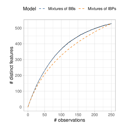
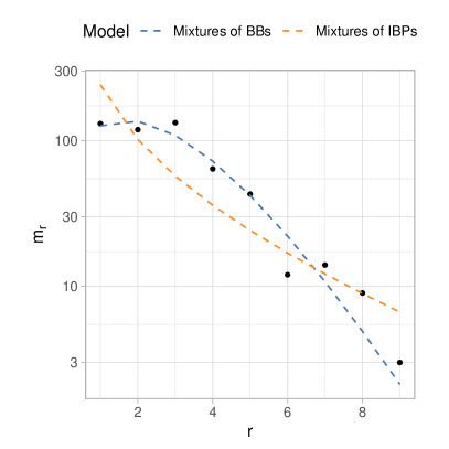
Figure S1: Case $n=250$. Left panel: the empirical accumulation curve (black dots) and the rarefaction curve of the models (blue and orange dashed lines). Right panel: the observed values of $K_{n,r}$ (black dots) compared with the expected curves $\mathds{E}(K_{n,r})$ (blue and orange dashed lines) for $r=1,\ldots,9$.

Focusing on the prediction of the number of unseen features in an additional sample of increasing size, we compare the Poisson mixture of bbs, the negative binomial mixture of bbs, the frequentist estimator (Chao) in Chao et al. (2014) and a variation of the Good-Toulmin estimators (GT) in Chakraborty et al. (2019). For the negative binomial mixture of bbs, we analyse two distinct choices for the prior variance of $N$, specifically $\operatornamewithlimits{Var}(N)=\mu_{0}\times c$, with $c\in\{10,1000\}$. We report the comparison in Figure S2, for $n\in\{50,250\}$. In the case $n=50$, the point-wise estimates produced by our mixtures of bbs are rather good, definitely outperforming the ones obtained with the frequentist estimator in Chao et al. (2014), which underestimates the extrapolation curve. While the Good-Toulmin estimates seem pretty reliable in the case $n=50$, such an estimator shows bad predictive performance and well-known stability issues for $n=250$. Moreover, the mixtures of bbs allow us to quantify the uncertainty around the point estimates through credible intervals: this is a remarkable advantage of our Bayesian framework. Observe that the credible bands contain the observed curve in the test set; for $n=50$ it is evident how the negative binomial mixtures account for larger dispersion than the Poisson mixture, having wider credible intervals. For completeness, the sanity check in the larger sample $n=1250$, where $k=599$ features are observed, is satisfactory: the credible interval of $K_{m}^{(n)}+k\mid\bm{Z}^{(n)}$, for $m=300$, is $[599,601]$. Finally, we remark that, while both the frequentist estimators are exclusively designed for the specific extrapolation problem, our model-based approach through mixtures of bbs offers a coherent and self-contained framework for a number of inference problems, where the prediction of the number of unseen features is just one available example.

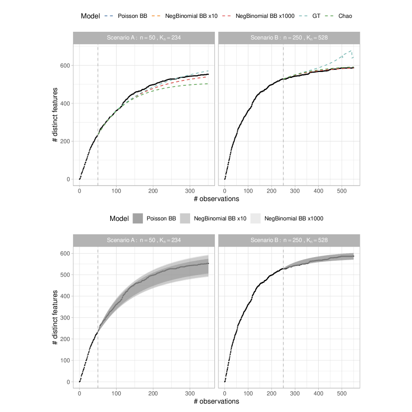
Figure S2: Top row: the accumulation curve $K_{m}^{(n)}+k\mid\bm{Z}^{(n)}$ under the two mixtures of bbs, the Good-Toulmin estimator and the Chao estimator for $n=50$ (left) and $n=250$ (right). Bottom row: the $95\%$ credible intervals of $K_{m}^{(n)}+k\mid\bm{Z}^{(n)}$, for $n=50$ (left) and $n=250$ (right), for the Poisson and the negative binomial mixtures of bbs. The grey vertical lines indicate the training set.

Additionally, mixtures of bbs also allow the estimation of the richness. We refer to Figure S3 for an insightful illustration on the richness estimation via the Poisson mixture and two negative binomial mixtures with $\operatornamewithlimits{Var}(N)=\mu_{0}\times c$, for $c\in\{10,1000\}$. Specifically, Figure S3 shows, for increasing sample sizes $n\in\{50,250,1250\}$, the posterior mean of the species richness $N$, for different choices of the parameters of the prior distribution on $N$. In particular, for each model, we estimate the parameters following the usual empirical Bayes procedure described in Section 6.1 (referred to as EB in the figure); moreover, we fix different choices for the prior mean of $N$, i.e., $\mathds{E}(N)\in\{200,400,800\}$, and we estimate the parameters $\alpha$ and $\theta$ as discussed in Section 6.1. We observe that, as the size $n$ of the training set increases, the richness estimates shrink towards the true value $H=600$. We also highlight that when prior guesses on $N$ are far from the truth, e.g., $\mathds{E}(N)\in\{200,400,800\}$, negative binomial mixtures of bbs with larger variances produce richness estimates that are closer to the true value $H$ than the ones produced by the Poisson mixture, due to the greater flexibility of the negative binomial prior, which gives less weight to prior guesses.

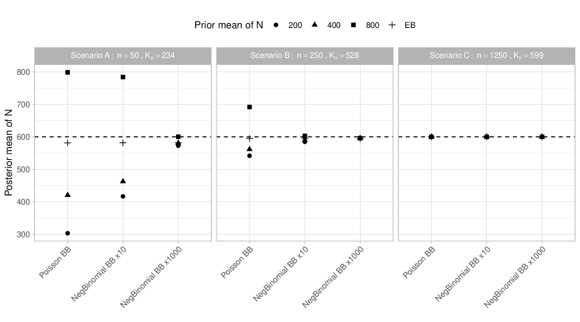
Figure S3: Posterior mean of the richness $N$, for increasing sample sizes $n\in\{50,250,1250\}$, and different values of the parameters of the models. The dashed lines indicate the true richness $H=600$.

Finally, in Figure S4, we show the posterior distributions of the richness $N$, reporting (i) the empirical Bayes approach for parameters elicitation and (ii) the prior mean of $N$ equal to $400$. Commenting on the inference produced in case (i), we observe that such posterior distributions give high probability mass to the true richness $H=600$; for smaller sample size $n=50$, we can highlight the higher dispersion of the posterior distribution of $N$ for the negative binomial mixtures. In case (ii), when the prior guess of $N$ is bad, e.g., $\mathds{E}(N)=400$, the inference gets worse as the sample size decreases, e.g., $n=50$. This is clearly expected since the posterior of $N$ gives more weight to the contribution of the prior, which brings an incorrect guess. However, it is interesting to note that the negative binomial mixture with larger prior variance for $N$, i.e., $\operatornamewithlimits{Var}(N)=1000\times\mu_{0}$, is perfectly catching the true richness even for $n=50$.

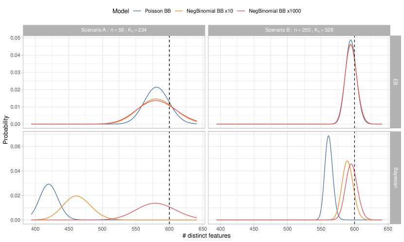
Figure S4: Posterior distribution of the richness $N$ for increasing sample sizes $n\in\{50,250\}$. Top row: parameters elicited according to the empirical Bayes approach; bottom row: $\mathds{E}(N)=400$, with $\alpha$ and $\theta$ chosen as in Section 6.1. The vertical black lines indicate the true richness $H=600$.

S4.2 Simulation study B

We assume a generating mechanism such that the feature occurrence probabilities $\pi_{k}$’s are set as $\pi_{k}=1/k$, for $k=1,\ldots,H$, with $H=10^{6}$ total features. The choice of a large $H$ is intended to mimic a scenario where the number of features is infinite. We generate a dataset of observations and we consider increasing dimensions of the training set $n\in\{10,50,250\}$. In Figure S5 we report the results of the suggested model-checking procedure for the case $n=50$. Differently from simulation study A, the mixtures of bbs are not properly fitting the data. Instead, we argue that the mixtures of ibps can be assumed to be correctly specified.

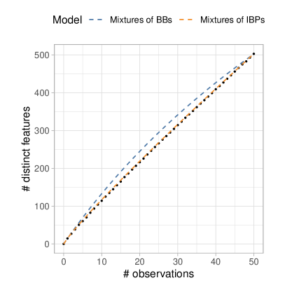
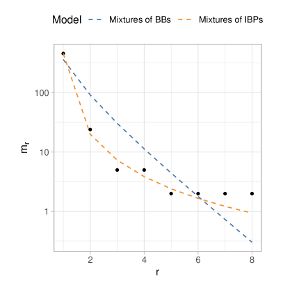
Figure S5: Case $n=50$. Left panel: the empirical accumulation curve (black dots) and the rarefaction curve of the models (blue and orange dashed lines). Right panel: the observed values of $K_{n,r}$ (black dots) compared with the expected curves $\mathds{E}(K_{n,r})$ (blue and orange dashed lines) for $r=1,\ldots,8$.

We address the prediction of the number of unseen features in an additional sample of increasing size, comparing the gamma mixture of ibps and a variation of the Good-Toulmin estimators (GT) in Chakraborty et al. (2019). We do not consider the estimator in Chao et al. (2014) here, since it is specifically designed for situations where the assumption of finite richness is plausible. For the gamma mixture of ibps, we consider two distinct choices for the prior variance of $\gamma$, i.e., $\operatornamewithlimits{Var}(\gamma)\in\{0.01,100\}$. We report the comparison in Figure S6, for $n\in\{10,50,250\}$. Starting with the Good-Toulmin estimates, it is evident how the prediction curve catches the observed curve just for very limited horizons $m$. On the other hand, both the gamma mixtures are able to capture the growth rate of $K^{(n)}_{m}$ for increasing values of $m$. Remarkably, a larger prior variance of $\gamma$, e.g., $\operatornamewithlimits{Var}(\gamma)=100$, results in wider credible intervals for the prediction, allowing for a more conservative uncertainty quantification. Indeed, when the prior variance is smaller, e.g., $\operatornamewithlimits{Var}(\gamma)=0.01$, the observed extrapolation curve is not always contained in the credible bands, leading to a less reliable prediction of the variability of the phenomenon. Remind that the limiting case $\operatornamewithlimits{Var}(\gamma)\to 0$ corresponds to the ibp model; this clearly justifies the need of the mixtures of ibps.

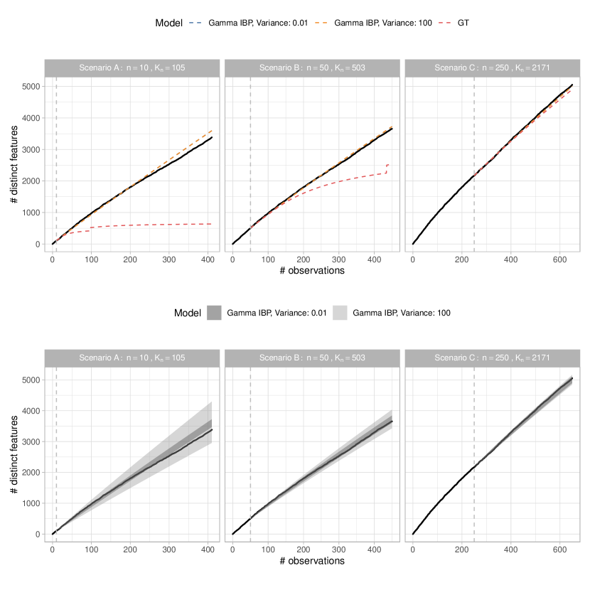
Figure S6: Top row: the accumulation curve $K_{m}^{(n)}+k\mid\bm{Z}^{(n)}$ under the gamma mixtures of ibps and the Good-Toulmin estimator for $n=10$ (left), $n=50$ (center) and $n=250$ (right). Bottom row: the $95\%$ credible intervals of $K_{m}^{(n)}+k\mid\bm{Z}^{(n)}$, for $n=10$ (left), $n=50$ (center) and $n=250$ (right), for the gamma mixtures of ibps.

S4.3 Simulation study C

Here, we report a simulation study where the data are generated from the bb model, with total number of features equal to $H=500$. Specifically, the feature occurrence probabilities are drawn as $\pi_{k}\stackrel{{\scriptstyle\textup{iid}}}{{\sim}}{\rm Beta}(1,100)$, $k=1,\ldots,H$. We generate a dataset of observations and we consider increasing dimensions of the training set $n\in\{200,1000,5000\}$. The sample sizes are larger than the other simulation studies since the growth of the accumulation curve is rather slow.

Figure S7 shows the model-checking for the case $n=1000$. As expected, the mixtures of ibps cannot explain the observed data. Conversely, it is reasonable to assume the mixtures of bbs to be correctly specified for this dataset. Therefore, we focus on the mixtures of bbs for the inference and prediction.

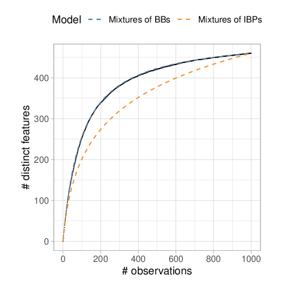
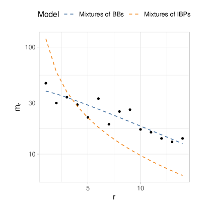
Figure S7: Case $n=1000$. Left panel: the empirical accumulation curve (black dots) and the rarefaction curve of the models (blue and orange dashed lines). Right panel: the observed values of $K_{n,r}$ (black dots) compared with the expected curves $\mathds{E}(K_{n,r})$ (blue and orange dashed lines) for $r=1,\ldots,14$.

Similarly to simulation study A, we compare the Poisson mixture of bbs, the negative binomial mixture of bbs, the frequentist estimator (Chao) in Chao et al. (2014) and a variation of the Good-Toulmin estimators (GT) in Chakraborty et al. (2019), in terms of prediction of the number of unseen features in an additional sample of increasing size. For the negative binomial mixture of bbs, we analyse two distinct choices for the prior variance of $N$, specifically $\operatornamewithlimits{Var}(N)=\mu_{0}\times c$, with $c\in\{10,1000\}$. We report the comparison in Figure S8, for $n\in\{200,1000\}$. For larger sample sizes, e.g., $n=1000$, all the models seem to produce reliable predictions, at least for the analyzed horizon $m=1,\ldots,500$. Significant differences are observed for the smaller sample size $n=200$, where the point-wise estimates (the expected values of $K_{m}^{(n)}+k$, for $m=1,\ldots,500$) produced by our mixtures of bbs accurately predict the observed curve in the test set, with the credible intervals nicely quantifying the uncertainty around such estimates. Indeed, the observed curve is always contained in the credible bands. On the other hand, the Good-Toulmin estimates show their well-known stability issues, while the estimator in Chao et al. (2014) clearly underestimates the observed curve.

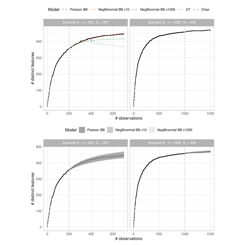
Figure S8: Top row: the accumulation curve $K_{m}^{(n)}+k\mid\bm{Z}^{(n)}$ under the two mixtures of bbs, the Good-Toulmin estimator and the Chao estimator for $n=200$ (left) and $n=1000$ (right). Bottom row: the $95\%$ credible intervals of $K_{m}^{(n)}+k\mid\bm{Z}^{(n)}$, for $n=200$ (left) and $n=1000$ (right), for the Poisson and the negative binomial mixtures of bbs. The grey vertical lines indicate the training set.

For the analyzed dataset, the model-checking in Figure S7 suggests the correct specification of the mixtures of bbs. Consequently, it is reasonable to assume the finiteness of the richness and address its estimation. Figure S9 shows an expected, still remarkable, illustration on the richness estimation via the Poisson mixture and two negative binomial mixtures with $\operatornamewithlimits{Var}(N)=\mu_{0}\times c$, with $c\in\{10,1000\}$. Specifically, for increasing sample sizes $n\in\{200,1000,5000\}$, it reports the posterior mean of the species richness $N$, for different choices of the parameters of the prior distribution on $N$. In particular, for each model, we estimate the parameters following the usual empirical Bayes procedure (referred to as EB in the figure); moreover, we fix different choices for the prior mean of $N$, i.e., $\mathds{E}(N)\in\{200,400,800\}$, and we estimate the parameters $\alpha$ and $\theta$ as discussed in Section 6.1. We observe that, as the size $n$ of the training set increases, the richness estimates shrink towards the true value $H=500$. We also highlight that when prior guesses on $N$ are substantially wrong, e.g., $\mathds{E}(N)\in\{200,400,800\}$, negative binomial mixtures of bbs with larger variances produce richness estimates that are closer to the true value $H$ than the ones produced by the Poisson mixture, due to the greater flexibility of the negative binomial prior, which is able to give less weight to wrong prior guesses.

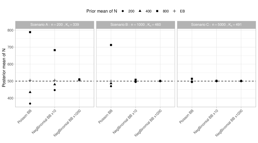
Figure S9: Posterior mean of the richness $N$, for increasing sample sizes $n\in\{200,1000,5000\}$, and different values of the parameters of the models. The dashed lines indicate the true richness $H=500$.

Finally, in Figure S10, we show the posterior distributions of the richness $N$, reporting (i) the empirical Bayes approach for parameters elicitation and (ii) the prior mean of $N$ equal to $400$. Commenting on the inference produced in case (i), we observe that such posterior distributions give high probability mass to the true richness $H=500$; for smaller sample size $n=200$, we can remark the higher dispersion of the posterior distribution of $N$ for the negative binomial mixtures. In case (ii), when the prior guess of $N$ is wrong, e.g., $\mathds{E}(N)=400$, the inference gets worse as the sample size decreases, e.g., $n=200$. This is clearly expected since the posterior of $N$ gives more weight to the contribution of the prior, which brings an incorrect guess. However, It is interesting to note how the negative binomial mixtures are perfectly catching the true richness even for $n=200$.

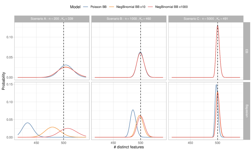
Figure S10: Posterior distribution of the richness $N$ for increasing sample sizes $n\in\{200,1000,5000\}$. Top row: parameters elicited according to the empirical Bayes approach; bottom row: $\mathds{E}(N)=400$, with $\alpha$ and $\theta$ chosen as in Section 6.1. The vertical black lines indicate the true richness $H=500$.

S5 Ecological applications: additional details and fully Bayesian approach

S5.1 Additional plots

In the present section we report the two taxon accumulation curves for the data considered in Section 7 of the main paper. Figure S11 shows the taxon accumulation for the vascular plants in Mazziotta et al. (2016a); Figure S12 illustrates the same curve for the Barro Colorado Island dataset, freely available in the vegan package in R. In both cases, the plots clearly indicate that the asymptote of the curve has not yet been reached, suggesting that the species richness will exceed the observed number of species in the sample.

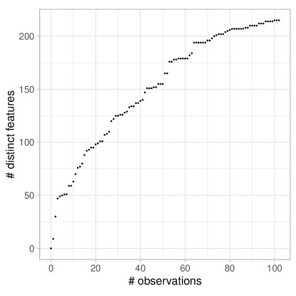
Figure S11: Taxon accumulation curve for the vascular plants in Mazziotta et al. (2016a).

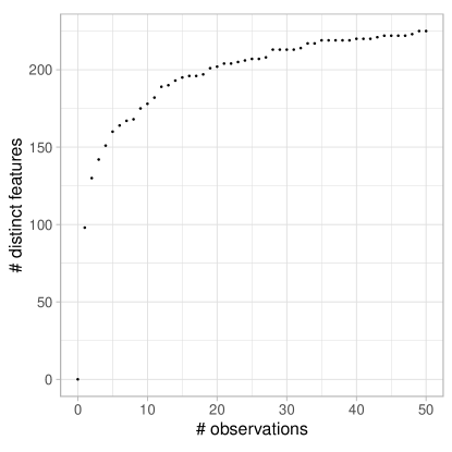
Figure S12: Taxon accumulation curve for the trees in the Barro Colorado Island data.

S5.2 Fully Bayesian approach: details

In Section 6.1 we describe a recommended procedure for eliciting the parameters of the models via an empirical Bayes approach. We consider such a procedure for all the discussed simulation studies and real data examples. However, one might prefer to adopt a fully Bayesian approach instead of the proposed empirical Bayes one. Specifically, the interest might be in assuming prior distributions for the parameters $\alpha$ and $\theta$, for all of the mixtures. Within the mixtures of bbs, we argue that the negative binomial mixture has to be regarded as the fully Bayesian version of the Poisson mixture, since the former is obtained by placing a gamma prior on the $\lambda$ parameter of the latter.

In this section, we first discuss the prior elicitation for the parameters $\alpha$ and $\theta$; then, we illustrate the comparison with the empirical Bayes approach, in terms of inference and prediction obtained in the two real data scenarios. As far as prior elicitation is concerned, since the constraint $\theta>-\alpha$ for all of the models, it is convenient to perform a change of variable, introducing $s=\theta+\alpha$ and removing $\theta$, so that $s>0$. Then, prior distributions on $\alpha$ and $s$ are specified. Specifically, for the mixtures of ibps, characterized by $\alpha\in[0,1)$, we consider

$$\alpha\sim{\rm Beta}\left(a_{\alpha},b_{\alpha}\right),\;s\sim{\rm Gamma}\left(a_{s},b_{s}\right),$$

with $a_{\alpha},b_{\alpha}>0$ and $a_{s},b_{s}>0$. Denoting with $\hat{\alpha}$ and $\hat{\theta}$ the empirical Bayes estimates obtained as in Section 6.1, we select the hyperparameters of the priors by imposing $\mathds{E}(\alpha)=\hat{\alpha}$ and $\mathds{E}(s)=\hat{s}$, where $\hat{s}=\hat{\alpha}+\hat{\theta}$. It follows that $a_{\alpha}/(a_{\alpha}+b_{\alpha})=\hat{\alpha}$ and $a_{s}/b_{s}=\hat{s}$. Two additional equations, one involving $a_{\alpha},b_{\alpha}$ and one involving $a_{s},b_{s}$, are necessary to fix the four hyperparameters. For example, such equations may control the prior variances of $\alpha$ and $s$, so that the practitioner can select the degree of regularization induced by the priors. Draws from the posterior distribution of $(\alpha,s)$ can be easily obtained via any Metropolis-Hastings algorithm. Specifically, we apply the change of variables $\alpha^{\prime}=\log(\alpha/(1-\alpha))$, $s^{\prime}=\log(s)$, so that $(\alpha^{\prime},s^{\prime})\in\mathds{R}^{2}$, and we update $(\alpha^{\prime},s^{\prime})$ via a pre-conditioned MALA (Metropolis Adjusted Langevin Algorithm), since the gradient of the log-full-conditional density of $(\alpha^{\prime},s^{\prime})$ is available in closed form.

For the mixtures of bbs, having $\alpha<0$, we consider

$$-\alpha\sim{\rm Gamma}\left(a_{\alpha},b_{\alpha}\right),\;s\sim{\rm Gamma}\left(a_{s},b_{s}\right),$$

with $a_{\alpha},b_{\alpha}>0$ and $a_{s},b_{s}>0$. We choose the hyperparameters of the priors such that $\mathds{E}(\alpha)=\hat{\alpha}$ and $\mathds{E}(s)=\hat{s}$. This imposes $a_{\alpha}/b_{\alpha}=-\hat{\alpha}$ and $a_{s}/b_{s}=\hat{s}$. Similarly to the mixtures of ibps, one may set the degree of regularization induced by the priors by choosing the prior variances of $\alpha$ and $s$. Sampling from the posterior distribution of $(\alpha,s)$ is straightforward through any Metropolis-Hastings algorithm. We resort again to a pre-conditioned MALA for the transformed parameters $(\alpha^{\prime},s^{\prime})$, where $\alpha^{\prime}=\log(-\alpha)$, $s^{\prime}=\log(s)$, and we stress that the gradient of the log-full-conditional density of $(\alpha^{\prime},s^{\prime})$ is available in closed form.

Here, we report the comparison among the fully Bayesian approach and the empirical Bayes approach described in Section 6.1, in terms of inference and/or prediction, concerning the two real data scenarios.

Vascular plants in Danish forest.

Analyzing the vascular plants data of Mazziotta et al. (2016a) in Section 7.1, we claimed the correct specification of the mixtures of ibps. We consequently showed the prediction obtained via the gamma mixture of ibps, using the empirical Bayes approach to select the parameters. In particular, the empirical Bayes estimates for $\alpha$ and $\theta$ result as follows: $\hat{\alpha}=0.17$, $\hat{\theta}=1.7$. For the fully Bayesian approach, we then select the hyperparameters by imposing: $\mathds{E}(\alpha)=\hat{\alpha}=0.17$, $\operatornamewithlimits{Var}(\alpha)=10^{-2}$, and $\mathds{E}(s)=\hat{s}=1.87$, $\operatornamewithlimits{Var}(s)=187$, so that a moderate amount of regularization is introduced. We run the MCMC algorithm for $5\cdot 10^{4}$ iterations, discarding the first $5\cdot 10^{3}$ and keeping one every two iterations. In Figure S13, we report the comparison between the fully Bayesian approach and the empirical Bayes approach described in Section 6.1, in terms of the extrapolation curve. We observe that, for both the choices of the prior variance of $\gamma$, the expected number of unseen species which will be collected in additional samples of increasing sizes $m$ is almost identical for the two approaches. This is desirable since it confirms that the empirical Bayes approach leads to equivalent prediction than the fully Bayesian procedure. On the other hand, the credible intervals produced by the fully Bayesian approach are larger than the ones estimated with the empirical Bayes method, as naturally expected.

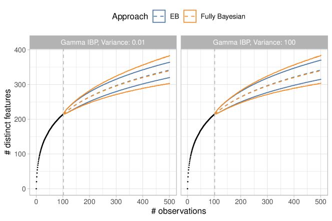
Figure S13: Comparison between the empirical Bayes approach (EB) and the fully Bayesian approach in terms of expected values and the $95\%$ credible intervals for $K_{m}^{(n)}+k$, with $k=215$, for the gamma mixtures of ibps. The extrapolation horizon is $m=1,\ldots,400$. The left panel shows the case $\operatornamewithlimits{Var}(\gamma)=0.01$, the right panel considers $\operatornamewithlimits{Var}(\gamma)=100$.

Trees in Barro Colorado Island.

Differently than for the vascular plants of Mazziotta et al. (2016a), the tree data investigated in Section 7.2 are suitably modelled via the mixtures of bbs (refer to Figure 5). In the main text, we report the inference and prediction produced by the Poisson and negative binomial mixtures of bbs, with parameters selected via the empirical Bayes approach discussed in Section 6.1. In particular, we get $\hat{\alpha}=-0.29$ and $\hat{\theta}=0.95$ as empirical Bayes estimates for the parameters. In the fully Bayesian approach, we select the hyperparameters so that $\mathds{E}(\alpha)=\hat{\alpha}=-0.29$, $\operatornamewithlimits{Var}(\alpha)\approx 300$, and $\mathds{E}(s)=\hat{s}=0.66$, $\operatornamewithlimits{Var}(s)\approx 650$. We run the MCMC algorithm for $5\cdot 10^{4}$ iterations, discarding the first $5\cdot 10^{3}$ and keeping one every two iterations. In Figure S14, we report the comparison between the fully Bayesian approach and the empirical Bayes approach, in terms of the extrapolation curve. The expected values for the extrapolation curve are similar between the two approaches, with larger credible intervals in the fully Bayesian case. This behavior is expected and desired. Moreover, Figure S15 shows the posterior distribution of $N$, the species richness, under the different approaches. It is evident that the fully Bayesian approach leads to much more dispersed posterior distributions for $N$. In particular, we remind that the empirical Bayes procedure estimates an expected species richness of $296.17$, with credible interval $[278,316]$, for both the choices of the prior variance of $N$. The fully Bayesian approach produces an expected species richness of $306$ with credible interval $[262,375]$, for the case $\operatornamewithlimits{Var}(N)=10\times\mu_{0}$, while it leads to an expected species richness of $320$ with credible interval $[262,447]$, for the case $\operatornamewithlimits{Var}(N)=1000\times\mu_{0}$.

Figure S14: Comparison between the empirical Bayes approach (EB) and the fully Bayesian approach in terms of expected values and the $95\%$ credible intervals for $K_{m}^{(n)}+k$, with $k=225$, for the negative binomial mixtures of bbs. The extrapolation horizon is $m=1,\ldots,400$. The left panel shows the case $\operatornamewithlimits{Var}(N)=10\times\mu_{0}$, the right panel considers $\operatornamewithlimits{Var}(N)=1000\times\mu_{0}$.

Figure S15: Comparison between the empirical Bayes approach (EB) and the fully Bayesian approach in terms of the posterior distribution of the species richness $N$, for the negative binomial mixtures of bbs. The left panel shows the case $\operatornamewithlimits{Var}(N)=10\times\mu_{0}$, the right panel considers $\operatornamewithlimits{Var}(N)=1000\times\mu_{0}$.

References

• Ayed and Caron (2021) Ayed, F. and F. Caron (2021). Nonnegative Bayesian nonparametric factor models with completely random measures. Statistics and Computing 31(5), 31–63.
• Battiston et al. (2018) Battiston, M., S. Favaro, D. M. Roy, and Y. W. Teh (2018). A characterization of product-form exchangeable feature probability functions. The Annals of Applied Probability 28(3), 1423–1448.
• Broderick et al. (2012) Broderick, T., M. I. Jordan, and J. Pitman (2012). Beta processes, stick-breaking and power laws. Bayesian Analysis 7(2), 439–476.
• Broderick et al. (2015) Broderick, T., L. Mackey, J. Paisley, and M. I. Jordan (2015). Combinatorial clustering and the beta negative binomial process. IEEE Trans. Pattern Anal. Mach. Intell. 37(2), 290–306.
• Broderick et al. (2013) Broderick, T., J. Pitman, and M. Jordan (2013). Feature allocations, probability functions, and paintboxes. Bayesian Analysis 8(4), 801–836.
• Camerlenghi et al. (2024) Camerlenghi, F., S. Favaro, L. Masoero, and T. Broderick (2024). Scaled process priors for Bayesian nonparametric estimation of the unseen genetic variation. Journal of the American Statistical Association 119(545), 320–331.
• Chakraborty et al. (2019) Chakraborty, S., A. Arora, C. B. Begg, and R. Shen (2019). Using somatic variant richness to mine signals from rare variants in the cancer genome. Nature Communications 10, 5506.
• Chao et al. (2014) Chao, A., N. J. Gotelli, T. C. Hsieh, E. L. Sander, K. H. Ma, R. K. Colwell, and A. M. Ellison (2014). Rarefaction and extrapolation with hill numbers: a framework for sampling and estimation in species diversity studies. Ecological Monographs 84(1), 45–67.
• Chiu (2022) Chiu, C.-H. (2022). Incidence-data-based species richness estimation via a beta-binomial model. Methods in Ecology and Evolution 13(11), 2546–2558.
• Chiu (2023) Chiu, C. H. (2023). Sample coverage estimation, rarefaction, and extrapolation based on sample-based abundance data. Ecology 104(8), 1–15.
• Chiu et al. (2014) Chiu, C.-H., Y.-T. Wang, B. A. Walther, and A. Chao (2014). An improved nonparametric lower bound of species richness via a modified Good-Turing frequency formula. Biometrics 70(3), 671–682.
• Colwell (2009) Colwell, R. (2009). Biodiversity: concepts, patterns, and measurement, pp. 257–263. Princeton University Press.
• Colwell et al. (2012) Colwell, R. K., A. Chao, N. J. Gotelli, S.-Y. Lin, C. X. Mao, R. L. Chazdon, and J. T. Longino (2012, 03). Models and estimators linking individual-based and sample-based rarefaction, extrapolation and comparison of assemblages. Journal of Plant Ecology 5(1), 3–21.
• Daley and Vere-Jones (2008) Daley, D. J. and D. Vere-Jones (2008). An introduction to the theory of point processes. Vol. II (Second ed.). Probability and its Applications (New York). Springer, New York. General theory and structure.
• De Blasi et al. (2015) De Blasi, P., S. Favaro, A. Lijoi, R. H. Mena, I. Prunster, and M. Ruggiero (2015). Are Gibbs-type priors the most natural generalization of the Dirichlet process? IEEE Trans. Pattern Anal. Mach. Intell. 37(2), 212–229.
• De Blasi et al. (2013) De Blasi, P., A. Lijoi, and I. Prünster (2013). An asymptotic analysis of a class of discrete nonparametric priors. Statist. Sin. 23(3), 1299–1321.
• de Finetti (1937) de Finetti, B. (1937). La prévision : ses lois logiques, ses sources subjectives. Annales de l’Institut Henri Poincaré 7(1), 1–68.
• Erdélyi and Tricomi (1951) Erdélyi, A. and F. G. Tricomi (1951). The asymptotic expansion of a ratio of gamma functions. Pacific Journal of Mathematics 1(1), 133 – 142.
• Favaro et al. (2009) Favaro, S., A. Lijoi, R. H. Mena, and I. Prünster (2009). Bayesian non-parametric inference for species variety with a two-parameter Poisson-Dirichlet process prior. Journal of the Royal Statistical Society: Series B (Methodological) 71(5), 993–1008.
• Ferguson (1973) Ferguson, T. S. (1973). A Bayesian analysis of some nonparametric problems. The Annals of Statistics 1, 209–230.
• Gnedin (2010) Gnedin, A. (2010). A species sampling model with finitely many types. Electron. Commun. Probab. 15, 79–88.
• Gnedin and Pitman (2005) Gnedin, A. and J. Pitman (2005). Exchangeable Gibbs partitions and Stirling triangles. Zapiski Nauchnykh Seminarov, POMI 325, 83–102.
• Good (1953) Good, I. J. (1953). The population frequencies of species and the estimation of population parameters. Biometrika 40, 237–264.
• Good and Toulmin (1956) Good, I. J. and G. H. Toulmin (1956). The number of new species, and the increase in population coverage, when a sample is increased. Biometrika 43, 45–63.
• Gotelli and Colwell (2001) Gotelli, N. J. and R. K. Colwell (2001). Quantifying biodiversity: procedures and pitfalls in the measurement and comparison of species richness. Ecol. Lett. 4(4), 379–391.
• Gregoire (1984) Gregoire, G. (1984). Negative binomial distributions for point processes. Stoch. Proc. Appl. 16(2), 179–188.
• Griffiths and Ghahramani (2006) Griffiths, T. and Z. Ghahramani (2006). Infinite latent feature models and the Indian buffet process. In Y. Weiss, B. Schölkopt, and J. Platt (Eds.), Advances in Neural Information Processing Systems, Volume 18, pp.  475–482. MIT Press.
• Griffiths and Ghahramani (2011) Griffiths, T. L. and Z. Ghahramani (2011). The Indian buffet process: an introduction and review. Journal of Machine Learning Research 12, 1185–1224.
• Heaukulani and Roy (2020) Heaukulani, C. and D. M. Roy (2020). Gibbs-type Indian buffet processes. Bayesian Analysis 15(3), 683–710.
• Hjort (1990) Hjort, N. L. (1990). Nonparametric Bayes estimators based on beta processes in models for life history data. The Annals of Statistics 18(3), 1259–1294.
• James (2017) James, L. F. (2017). Bayesian Poisson calculus for latent feature modeling via generalized Indian buffet process priors. The Annals of Statistics 45(5), 2016–2045.
• Kim (1999) Kim, Y. (1999). Nonparametric Bayesian estimators for counting processes. The Annals of Statistics 27(2), 562–588.
• Kingman (1967) Kingman, J. F. C. (1967). Completely random measures. Pacific Journal of Mathematics 21, 59–78.
• Knowles and Ghahramani (2011) Knowles, D. and Z. Ghahramani (2011). Nonparametric Bayesian sparse factor models with application to gene expression modeling. The Annals of Applied Statistics 5(2B), 1534–1552.
• Lee et al. (2023) Lee, J., X. Miscouridou, and F. Caron (2023). A unified construction for series representations and finite approximations of completely random measures. Bernoulli 29(3), 2142–2166.
• Lijoi et al. (2007a) Lijoi, A., R. H. Mena, and I. Prünster (2007a). Bayesian nonparametric estimation of the probability of discovering new species. Biometrika 94(4), 769–786.
• Lijoi et al. (2007b) Lijoi, A., R. H. Mena, and I. Prünster (2007b). Controlling the reinforcement in Bayesian non-parametric mixture models. Journal of the Royal Statistical Society: Series B (Methodological) 69(4), 715–740.
• Lijoi and Prünster (2010) Lijoi, A. and I. Prünster (2010). Models beyond the Dirichlet process. In Bayesian nonparametrics, Volume 28 of Camb. Ser. Stat. Probab. Math., pp.  80–136. Cambridge Univ. Press, Cambridge.
• Magurran and McGill (2011) Magurran, A. E. and B. J. McGill (2011). Biological Diversity: frontiers in measurement and assessment. Oxford Biology.
• Masoero et al. (2022) Masoero, L., F. Camerlenghi, S. Favaro, and T. Broderick (2022). More for less: predicting and maximizing genomic variant discovery via Bayesian nonparametrics. Biometrika 109(1), 17–32.
• Mazziotta et al. (2016a) Mazziotta, A., J. Heilmann-Clausen, H. H. Bruun, O. Fritz, E. Aude, and A. P. Tøttrup (2016a). Dataset on species incidence, species richness and forest characteristics in a danish protected area. Data in Brief 9, 895–897.
• Mazziotta et al. (2016b) Mazziotta, A., J. Heilmann-Clausen, H. H. Bruun, O. Fritz, E. Aude, and A. P. Tøttrup (2016b). Restoring hydrology and old-growth structures in a former production forest: Modelling the long-term effects on biodiversity. For. Ecol. Manag. 381, 125–133.
• Miller et al. (2009) Miller, K. T., T. L. Griffiths, and M. I. Jordan (2009). Nonparametric latent feature models for link prediction. In Advances in Neural Information Processing Systems 22 (NIPS 2009), pp.  719–726.
• Nguyen et al. (2023) Nguyen, T. D., J. Huggins, L. Masoero, L. Mackey, and T. Broderick (2023). Independent finite approximations for Bayesian nonparametric inference. Bayesian Analysis In press.
• Palla et al. (2012) Palla, K., D. A. Knowles, and Z. Ghahramani (2012). An infinite latent attribute model for network data. In Proceedings of the 29th International Coference on International Conference on Machine Learning, Madison, WI, USA, pp. 395–402. Omnipress.
• Pitman (1996) Pitman, J. (1996). Some developments of the Blackwell-MacQueen urn scheme. In Statistics, probability and game theory, Volume 30 of IMS Lecture Notes Monogr. Ser., pp.  245–267. Inst. Math. Statist., Hayward, CA.
• Pitman (2003) Pitman, J. (2003). Poisson-Kingman partitions. Lecture Notes-Monograph Series 40, 1–34.
• Pitman and Yor (1997) Pitman, J. and M. Yor (1997). The two-parameter Poisson-Dirichlet distribution derived from a stable subordinator. The Annals of Probability 25(2), 855–900.
• Quintana et al. (2022) Quintana, F. A., P. Müller, A. Jara, and S. N. MacEachern (2022). The Dependent Dirichlet Process and Related Models. Statistical Science 37(1), 24–41.
• Stolf and Dunson (2024) Stolf, F. and D. B. Dunson (2024). Allowing growing dimensional binary outcomes via the multivariate probit Indian buffet process. arXiv:2402.13384.
• Teh and Gorur (2009) Teh, Y. and D. Gorur (2009). Indian buffet processes with power-law behavior. In Y. Bengio, D. Schuurmans, J. Lafferty, C. Williams, and A. Culotta (Eds.), Advances in Neural Information Processing Systems, Volume 22.
• Teh and Jordan (2010) Teh, Y. W. and M. I. Jordan (2010). Hierarchical bayesian nonparametric models with applications. In Bayesian nonparametrics, Volume 28 of Camb. Ser. Stat. Probab. Math., pp.  158–207. Cambridge Univ. Press, Cambridge.
• Thibaux and Jordan (2007) Thibaux, R. and M. I. Jordan (2007). Hierarchical beta processes and the Indian buffet process. In Proceedings of the Eleventh International Conference on Artificial Intelligence and Statistics, Volume 2, pp.  564–571.
• Williamson et al. (2010) Williamson, S., C. Wang, K. A. Heller, and D. M. Blei (2010). The IBP compound Dirichlet process and its application to focused topic modeling. In Proceedings of the 27th International Conference on International Conference on Machine Learning, ICML’10, Madison, WI, USA, pp.  1151–1158. Omnipress.
• Zito et al. (2023a) Zito, A., T. Rigon, and D. B. Dunson (2023a). Bayesian nonparametric modeling of latent partitions via Stirling-gamma priors. arXiv:2306.02360.
• Zito et al. (2023b) Zito, A., T. Rigon, and D. B. Dunson (2023b). Inferring taxonomic placement from DNA barcoding aiding in discovery of new taxa. Methods in Ecology and Evolution 14(2), 529–542.
• Zito et al. (2023) Zito, A., T. Rigon, O. Ovaskainen, and D. B. Dunson (2023). Bayesian modeling of sequential discoveries. Journal of the American Statistical Association 188(544), 2521–2532.