Adiabatic and diabatic responses in a Duffing resonator driven by two detuned tones

Abstract

The combination of a strong pump and a weak probe has been widely applied to investigate both optical and nanomechanical devices. Such pump-probe measurements allows for the exploration of nonlinear dynamics, driven by the large pump tone, by measuring the system response to a probe tone. In contrast, here we report on the dynamics of a mechanical Duffing resonator driven with a combination of two large tones at different frequencies. Our results indicate the presence of variuos distinct regimes with very different dynamics. We systematically investigate the impact of the relative strength and detuning between the two drives on the dynamical response. This provides an illustrative example of dynamical phase transitions in out-of-equilibrium systems.

Measuring the response of a system to a strong ‘pump’ by means of a weak ‘probe’ has been a cornerstone of optical spectroscopy and microscopy for many years [1, 2, 3, 4]. In nanomechanics, pump-probe measurements are used to investigate the coupling between vibrational modes [5, 6, 7], study isolating electronic states in carbon nanotubes [8], and quantify the phase noise squeezing of a resonator [9]. In all these experiments, the probe amplitude is kept small to only explore linear perturbations of the system around the dominant pump-driven physics [10]. This condition separates the impact of the pump tone (sets the stationary state) from the probe (induces small fluctuations), making the method versatile and simple to interpret.

While useful for linear systems, the separation of the driving tones into so-called pump and probe severely restricts applications in nonlinear systems. There, both tones combined may lead to significant effects that cannot be analyzed separately [11, 12, 13, 14, 5, 7, 15]. For example, the interplay of the nonlinearity with multiple driving tones is responsible for phenomena such as strong optomechanical squeezing [16, 17], pulse-width modulation [18], parametric symmetry breaking [19], and even chaos [20]. In the latter two examples, the second tone drives instabilities in the system, leading to new dynamics that are challenging to describe analytically [21, 22]. In such a setting, the timescale of the beating between the drives relative to relaxation times in the system plays a crucial role in the resulting dynamics.

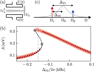
Figure 1: Experimental setup. (a) Simplified sketch of the tuning fork resonator (light grey) vibrating with amplitude $z_{i}$ in response to a voltage signal $U(t)$. The capacitive coupling to the lower electrode converts the vibration into an electrical signal $x(t)$. The tuning fork is biased with a voltage $U_{\mathrm{b}}=$32\text{\,}\mathrm{V}$$ is a bias voltage. (b) Measured amplitude response $A$ to a single driving tone $U=$140\text{\,}\mathrm{m}\mathrm{V}$$ swept from low to high (high to low) frequency $\Omega_{1}$ as filled (empty) dots, with $\Delta_{10}=\Omega_{1}-\Omega_{0}$. The dark solid (dashed) lines represent the analytical stationary stable (unstable) solutions, cf. Eqs. (2). Grey spheres highlight the position of the bifurcation points, cf. Eq. (3), and the grey vertical line corresponds to the tone frequency $\Delta_{10}/2\pi=$-148\text{\,}\mathrm{Hz}$$ used in Fig. 2. (c) Multi-tone experimental setup with a second tone frequency $\Omega_{2}$, detuned from the first tone by $\Delta_{21}=\Omega_{2}-\Omega_{1}$.

In this work, we test the response of a single Duffing (Kerr) resonator to a combination of two drive tones at different frequencies, which can be of comparable strength. We measure the response of the system by systematically varying the relative strength and detuning of the second tone. Under particular conditions, the system response is characterized by periodic orbits in phase space around the stationary states of the nonlinear resonator if driven by one tone. These orbits arise an interplay between the two drives, multistability, and dissipation. We explain these orbits with a modified model of the Duffing resonator. Our results explain this key effect in multi-tone measurements, and lay the groundwork for future explorations of nonlinear networks.

Our experimental setup consists of a tuning fork resonator, made out of single-crystal silicon, which is capacitively coupled to two electrodes fabricated next to it [23]. A schematic of the setup is shown in Fig. 1(a). We employ the lowest mechanical mode, whose resonance frequency $\Omega_{0}$ and Duffing nonlinearity $\beta$ is tuned by applying a bias voltage $U_{\mathrm{b}}$. An oscillating voltage $U(t)$ results in a driving force. The resulting mechanical vibration amplitudes $z_{i}$ is converted into an oscillating electrical voltage $x(t)$. Under a strong drive, the response of the system is distinctly nonlinear and can be described by the equation of motion:

$$\ddot{x}(t)+\Omega_{0}^{2}x(t)+\Gamma\dot{x}(t)+\beta x^{3}(t)=F(t)\,,$$ (1)

with $\Gamma$ the damping rate, $F(t)=U(t)\times C$ the overall applied force in units of $\text{\,}\mathrm{V}\text{\,}{\mathrm{s}}^{-2}$ with a conversion factor $C\approx$1\text{\times}{10}^{7}\text{\,}{\mathrm{s}}^{-2}$$, and $\beta$ the negative (softening) Duffing coefficient. From calibration measurements, we obtain the parameters $\Omega_{0}/2\pi=1.109~{}\mathrm{MHz}$, $\Gamma/2\pi=110\,\mathrm{Hz}$, and $\beta=-1.89\times 10^{17}\,\mathrm{V}^{-2}\mathrm{s}^{-2}$ [24].

To characterize our system, we first measure the response of the resonator to a single external force $F(t)=F_{1}\cos{(\Omega_{1}t+\theta_{1})}$ with frequency $\Omega_{1}\approx\Omega_{0}$, fixed phase $\theta_{1}$ and strength $F_{1}/C=$140\text{\,}\mathrm{mV}$$. We generate the oscillating force and collect data with a lock-in amplifier (Zurich Instrument MFLI) set to a local oscillator frequency $\Omega_{1}$, enabling the down-conversion to extract the in-phase ($X$) and out-of-phase ($Y$) quadratures defined by $x(t)=X(t)\cos(\Omega_{1}t)-Y(t)\sin(\Omega_{1}t)$. In Fig. 1(b), we show the measured amplitude response at frequency $\Omega_{1}$, $A(t)=\sqrt{X(t)^{2}+Y(t)^{2}}$, for sweeps from low to high (high to low) frequencies as filled (empty) dots. In each sweep, we can see the system performing a jump between high and low amplitudes.

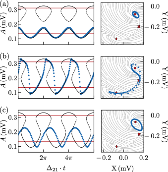
Figure 2: System response to two-tone drive. Measured amplitude $A(t)$ over time (left panel) for (a) $h=~{}0.14$ and $\Delta_{21}/2\pi=10~{}$\mathrm{H}\mathrm{z}$$, (b) $h=~{}0.21$ and $\Delta_{21}/2\pi=10~{}$\mathrm{H}\mathrm{z}$$, and (c) $h=~{}0.21$ and $\Delta_{21}/2\pi=90~{}$\mathrm{H}\mathrm{z}$$, where $h=F_{2}/F_{1}$. We initialize the system in the low-amplitude state with a fixed voltage $F_{1}/C=140~{}$\mathrm{m}\mathrm{V}$$ and $\Delta_{10}/2\pi\approx-148~{}$\mathrm{H}\mathrm{z}$$. Red lines and symbols indicate the analytical single-tone stationary solutions of the system for $h=0$: the disk and the diamond represent the high and low amplitude stable states, respectively, while the cross marks the unstable state. Grey lines in the phase space plot show the flow lines calculated for the same parameters. The dark solid (dashed) lines represent the calculated stable (unstable) stationary solutions of the Duffing equation with two drives, in the resonant limit $\Omega_{1}\approx\Omega_{2}$, cf. Eq. (2).

Next, we add a second weak probe tone, such that $F(t)=\sum_{m=1,2}F_{m}\cos{(\Omega_{m}t+\theta_{m})}$. We initialize the system in the low-amplitude stationary solution in Fig. 1(b) at a detuning $\Delta_{10}=\Omega_{1}-\Omega_{0}$, cf. Fig. 1(c). The second tone has an amplitude $F_{2}=hF_{1}$, and a frequency $\Omega_{2}$ detuned from $\Omega_{1}$ by $\Delta_{21}=\Omega_{2}-\Omega_{1}$. For $\Delta_{10}/2\pi=$-148\text{\,}\mathrm{Hz}$$, $h=0.14$, and $\Delta_{21}\approx 0.09\Gamma$, the response at $\Omega_{1}$ shows a small oscillation around the initial solution (red line and symbols in Fig. 2) at a frequency $\Delta_{21}$, see left panel in Fig. 2(a). In the frame rotating at $\Omega_{1}$, spanned by $X$ and $Y$, this oscillation forms a closed loop around the initial state, see right panel. Increasing the probe amplitude to $h=0.21$, we observe a striking change in the response character [18]. As shown in Fig. 2(b), the system exhibits large amplitude variations, with $X$ and $Y$ tracing an eight-shaped trajectory, which circles the two stable solutions the system has when driven only by $F_{1}$ ($h=0$). In the following, we refer to these solutions as ‘single-tone solutions’. Increasing the detuning $\Delta_{21}$ while keeping $h=0.21$ alters the response once more, see Fig. 2(c). Here, the system’s quadratures oscillate around one single-tone solution. This case differs from the similar phenomenon in Fig. 2(a), marking a third experimental regime with unique features discussed below.

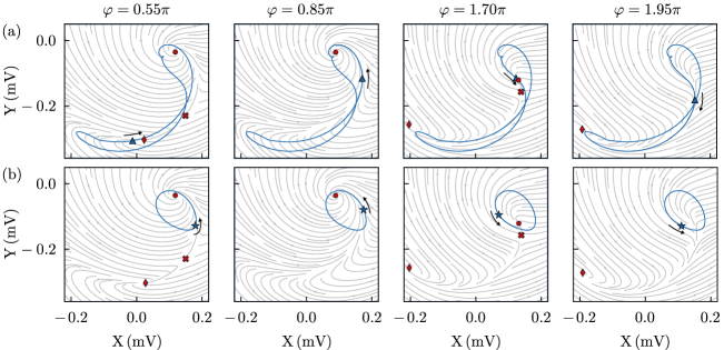
Figure 3: Theory analysis for the adiabatic and diabatic regime. (a) From left to right we show snapshots at various $\varphi$ (top labels), during a single modulation cycle of the adiabatic ($\Delta_{21}/2\pi=10\,\mathrm{Hz}$) regime. The instantaneous solution (blue triangle) adiabatically follows the high amplitude solution (red diamond), jumps to the low-amplitude solution (red disk), adiabatically follows the low-amplitude solution, and jumps to the high-amplitude solution. (b) Same snapshots in the diabatic ($\Delta_{21}/2\pi=90\,\mathrm{Hz}$) regime. Here, in contrast, the instantaneous solution (blue star) remains confined to a trajectory around the low-amplitude solution. Parameters are the same as in the corresponding experiments in Fig. 2, with $\varphi=\Delta_{21}t$. The analytically calculated positions of the two stable (red disk and diamond) and the unstable solution (red cross), as well as the instantaneous system position, are shown together with a numerical simulation of the entire trajectory (blue line). Grey lines represent the stationary flow lines analytically calculated from Eqs. (2).

To better understand the differences between the three cases, we write Eq. (1) in the rotating frame measured by the lock-in amplifier at the frequency of the first drive, yielding

with $f(t)=F_{1}e^{i\theta_{1}}+F_{2}e^{i(\varphi(t)+\theta_{2})}$. Assuming the quadratures $X(t),Y(t)$ vary slowly relative to the drive frequency $\Omega_{1}$, we average them over the oscillation period $2\pi/\Omega_{1}$. For Eq. (2) to hold, $|\beta|X^{2}/\left(\Omega_{1}^{2}\right)$, $\left|\Omega_{1}^{2}-\Omega_{0}^{2}\right|/\Omega_{1}^{2}$, and $\sqrt{\beta F_{m}^{2}/\Omega_{1}^{6}}$ must be $\ll 1$ [25], conditions always fulfilled by our experimental parameters. Furthermore, the relative phase between the forces is assumed to change slowly over time. As $\varphi(t)=\Delta_{21}t$, this sets a condition on the validity of Eqs. (2) relative to $\Delta_{21}$.

We now look at the predicted stationary response amplitude at frequency $\Omega_{1}$, $A$, to a single-drive ($h=0$), shown in Fig. 1(b). We benchmark this with the analytical solution retrieved from the solution to $\dot{X}=\dot{Y}=0$ in Eqs. (2) [24]. The positions of the measured hysteretic jumps in Fig. 1(b) are dictated by so-called bifurcation points, which occur when [24]

with $\tilde{\Delta}_{01}=\sqrt{\Omega_{0}^{2}-\Omega_{1}^{2}}$. The strength of the external driving force therefore defines the position of the two bifurcation frequencies.

The dynamics observed in Fig. 2(a) and (b) can be reproduced by the effective model in Eqs. (2). As the detuning between the two drives is relatively slow, $\Delta_{21}<\Gamma$, we solve the stationary response once more, but insert an effective single-tone drive with fixed value for the force and phase given by a snapshot of $f(t)$. Intuitively, we can understand the main effect of the two detuned drives as a single amplitude-modulated drive with

$$|f(t)|=F_{1}\sqrt{1+h^{2}+2h\cos(\theta_{1}-\theta_{2}-\varphi(t))}.$$ (4)

Within each period, the resonator experiences a force ranging from $F_{1}-F_{2}$ (drives are completely out of phase) to $F_{1}+F_{2}$ (drives are in phase). Since the driving strength is amplitude modulated, the bifurcation points are also modulated, cf. Eq. (3). If the modulation is strong enough, the number of stable solutions at $\Omega_{1}$ changes between 1 and 2 periodically.

In Fig. 2(a), the probe strength ($h=0.14$) is insufficient to push the system near a bifurcation point. As a consequence, the low-amplitude stable solution shown in the left panel never merges with the unstable solution, and the system remains trapped near the initial single-tone solution. The weak rotating effective force from Eqs. (2), along with the counterclockwise flow lines, guides the system into an orbit around this solution in phase space. In contrast, the increased probe strength ($h=0.21$) in Fig. 2(b) pushes both bifurcation frequencies across $\Omega_{1}$ within each period. Here, the system follows a stable solution until it vanishes at a bifurcation point, where it is forced to jump to the remaining solution. As a result, in phase space we observe the system orbiting around the two single-tone solutions. As the flow lines around these solutions have opposite chirality, the system follows an eight-shaped trajectory. Except during sudden transitions at bifurcations, the system changes much slower than the ringdown time, requiring $\Delta_{21}\ll\Gamma$, such that it smoothly adapts to changing conditions. We term this regime ‘adiabatic’.

This adiabatic regime, which we explore in Fig. 2(b), was also studied in Ref. [18]. It can be compared to an hourglass where all the sand collects on the lower side before being turned, or to so-called bursting oscillations observed in nonlinear coupled systems [26]. By contrast, in Fig. 2(c) we use $\Delta_{21}\approx\Gamma$. Even though the stationary solutions and flow lines are identical to the ones in Fig. 2(b), the system cannot probe them quickly enough. The jumps are never completed, and the system orbits the initial single-tone solution. We term this regime ‘diabatic’. This diabatic case contrasts with Fig. 2(a), as in the latter the system can follow a single stationary state adiabatically because that solution remains available during the entire period.

To emphasize the difference between the adiabatic regime in Fig. 2(b) and the diabatic regime in Fig. 2(c), Fig. 3 presents snapshots of the system’s trajectory at different points in time during a single period, with the full time-evolving vector flow shown in the background. The adiabatic regime is shown in Fig. 3(a), with flow lines and stationary solutions calculated at each time, and a simulated trajectory of the system obtained by numerically evolving Eqs. (2) over a longer time. Please note that the overall changes in the vector flow—manifesting as changes in the number of solutions and their local flow chirality—indicate topological transitions in the overall dynamics [27]. Like in the experiment in Fig. 2(b), we observe the characteristic eight-shaped trajectory due to the opposite chirality of the flow lines around the two solutions. Crucially, the adiabatic changes allow us to sense they underlying topology of phase space. In the diabatic regime in Fig. 3(b), instead, the topology of the flow lines is identical to the corresponding panels in Fig. 3(a). However, the simulated trajectory is strikingly different, trailing (but never quite catching up with) the low-amplitude solution or the changing topology of the vector field. The resulting small loop is similar to the corresponding experiment in Fig. 2(c).

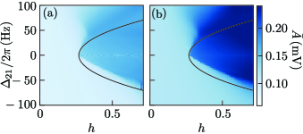
Figure 4: $\bar{A}$ for different detuning $\Delta_{21}$ and relative driving strength $h$. (a) Experimental results. (b) Numerical simulation. A low value indicates that the system remains close to the lower stable solution, while a high value indicates jumping between two solutions. To collect data and generate thes simulated value we used $F_{1}/C=$140\text{\,}\mathrm{mV}$$ and $\Delta_{10}/2\pi\approx$-158\text{\,}\mathrm{Hz}$$. A black line represents the analytical filter function given by Eq. (5). We attribute the discrepancy in amplitude between the experimental data and the simulation to a drift of the experimental resonance frequency.

The adiabatic-to-diabatic transition observed in Fig. 2 and simulated in Fig. 3 is governed by the competition between the amplitude-modulated drive and the resonator damping. In this competition, the finite energy decay rate $\Gamma$ of the resonator acts as a low-pass filter for the modulated drive relative to $\Omega_{1}$: it allows the slow transitions ($\Delta_{21}\ll\Gamma$) in Fig. 2(b) to pass, while blocking the fast transitions ($\Delta_{21}\approx\Gamma$) shown in Fig. 2(c). To substantiate this model, we systematically probe the response of the system as a function of $\Delta_{21}$ and $h$ for fixed $F_{1}$ and $\Omega_{1}$. For each combination, we extract the average value of the amplitude $\bar{A}$ from an interval of $5\text{\,}\mathrm{s}$. For a system initialized in the lower solution, this $\bar{A}$ is large when jumps to the high-amplitude solution take place, and small when the system explores only the vicinity of the initial low-amplitude solution.

In Fig. 4(a) and (b), we show $\bar{A}$ for different values of $\Delta_{21}$ and $h$ for both the experiment and a numerical simulation. We distinguish two main regions: low $\bar{A}$ where the second tone merely modulates the vibrational amplitude, without inducing jumps, cf. Fig. 2(a) and Fig. 2(c), and a high $\bar{A}$ region associated with jumping between the high- and low-amplitude solutions, cf. Fig. 2(b). The overall trend of both experiment and numerical simulation indicates that larger detuning $\Delta_{21}$, corresponding to faster modulation in the frame rotating at $\Omega_{1}$, requires higher drives $h$ to induce jumps. This is in agreement with the intuitive picture of a low-pass filter. There, the response of the system to the modulation is expected to be attenuated by a susceptibility function $\mathcal{F}(\Gamma,\Delta_{21})$. In order to force jumps, this attenuation must be compensated an increased critical modulation depth $h_{\mathrm{crit}}$ given by

$$h_{\mathrm{crit}}=\frac{1}{\mathcal{F}(\Gamma,\Delta_{21})}h_{0},$$ (5)

with $h_{0}$ the critical modulation depth for $\Delta_{21}=0$. We can analytically derive the function describing this competition between drive modulation and damping from an analysis of the averaged harmonic response to the probe field at the pump frequency [24], arriving at:

$$\mathcal{F}(\Gamma,\Delta_{21})=\frac{(\Gamma/2)^{2}}{(\Gamma/2)^{2}+\Delta_{21}^{2}}.$$ (6)

As shown by the black line in Fig. 4, the critical drive amplitude $h_{\mathrm{crit}}$ captures the overall shape of the experimental data and of the simulation results. However, at positive detuning, both experiment and simulation exhibit deviations from Eq. (5), which we attribute to nonlinear terms that are not considered in our simple filter function.

This work exemplifies the complex behavior of a Duffing resonator under the influence of two detuned drive tones. In particular, we highlight the transition from an adiabatic regime, where the system adheres to the underlying topology of the phase-space dynamics, to a diabatic regime where this is no longer true. The insights from this example are broadly applicable to other nonlinear systems, particularly to networks of nonlinear resonators, where the forces of the individual network constituents act as multiple drive tones that can induce many-body oscillation phases [28, 29, 30, 31]. Characterizing these phases in terms of their time-dependent phase-space topology [32, 27] and departures therefrom will provide a robust framework for sensing applications [18], computer vision [33], and kinematic synthesis in complex machinery [34]. Additionally, our work will drive further advancements in quantum hardware based on nonlinear resonators, where strong nonlinearity enables even more intricate mean-field solutions [35], crucial for ultimately generating complex quantum states, needed for quantum sensing [36] and error correction [37].

References

- Owyoung [1978] A. Owyoung, Coherent raman gain spectroscopy using cw laser sources, IEEE Journal of Quantum Electronics 14, 192 (1978).
- Lytle et al. [1985] F. Lytle, R. Parrish, and W. Barnes, An introduction to time-resolved pump/probe spectroscopy, Applied spectroscopy 39, 444 (1985).
- Tabosa et al. [1991] J. W. R. Tabosa, G. Chen, Z. Hu, R. B. Lee, and H. J. Kimble, Nonlinear spectroscopy of cold atoms in a spontaneous-force optical trap, Phys. Rev. Lett. 66, 3245 (1991).
- Mukamel [1995] S. Mukamel, Principles of nonlinear optical spectroscopy, Oxford University Press, New York (1995).
- Westra et al. [2010] H. J. R. Westra, M. Poot, H. S. J. van der Zant, and W. J. Venstra, Nonlinear modal interactions in clamped-clamped mechanical resonators, Phys. Rev. Lett. 105, 117205 (2010).
- Eichler et al. [2012] A. Eichler, M. del Álamo Ruiz, J. A. Plaza, and A. Bachtold, Strong coupling between mechanical modes in a nanotube resonator, Phys. Rev. Lett. 109, 025503 (2012).
- Antoni et al. [2012] T. Antoni, K. Makles, R. Braive, T. Briant, P.-F. Cohadon, I. Sagnes, I. Robert-Philip, and A. Heidmann, Nonlinear mechanics with suspended nanomembranes, EPL 100, 68005 (2012).
- Khivrich et al. [2019] I. Khivrich, A. A. Clerk, and S. Ilani, Nanomechanical pump–probe measurements of insulating electronic states in a carbon nanotube, Nature nanotechnology 14, 161 (2019).
- Ochs et al. [2021] J. S. Ochs, M. Seitner, M. I. Dykman, and E. M. Weig, Amplification and spectral evidence of squeezing in the response of a strongly driven nanoresonator to a probe field, Phys. Rev. A 103, 013506 (2021).
- Khitrova et al. [1988] G. Khitrova, P. R. Berman, and M. Sargent, Theory of pump–probe spectroscopy, JOSA B 5, 160 (1988).
- Boyd and Mukamel [1984] R. W. Boyd and S. Mukamel, Origin of spectral holes in pump-probe studies of homogeneously broadened lines, Phys. Rev. A 29, 1973 (1984).
- Eberly and Popov [1988] J. Eberly and V. Popov, Phase-dependent pump-probe line-shape formulas, Physical Review A 37, 2012 (1988).
- Gaižauskas and Valkūnas [1994] E. Gaižauskas and L. Valkūnas, Coherent transients of pump-probe spectroscopy in two-level approximation, Optics Communications 109, 75 (1994).
- Bonačić-Koutecký and Mitrić [2005] V. Bonačić-Koutecký and R. Mitrić, Theoretical Exploration of Ultrafast Dynamics in Atomic Clusters: Analysis and Control, Chemical Reviews 105, 11 (2005).
- Fani Sani et al. [2021] F. Fani Sani, I. C. Rodrigues, D. Bothner, and G. A. Steele, Level attraction and idler resonance in a strongly driven josephson cavity, Phys. Rev. Res. 3, 043111 (2021).
- Kronwald et al. [2013] A. Kronwald, F. Marquardt, and A. A. Clerk, Arbitrarily large steady-state bosonic squeezing via dissipation, Physical Review A 88, 063833 (2013).
- Zhang et al. [2022] W. Zhang, T. Wang, X. Han, S. Zhang, and H.-F. Wang, Mechanical squeezing induced by duffing nonlinearity and two driving tones in an optomechanical system, Physics Letters A 424, 127824 (2022).
- Houri et al. [2019] S. Houri, R. Ohta, M. Asano, Y. M. Blanter, and H. Yamaguchi, Pulse-width modulated oscillations in a nonlinear resonator under two-tone driving as a means for mems sensor readout, Japanese Journal of Applied Physics 58, SBBI05 (2019).
- Leuch et al. [2016] A. Leuch, L. Papariello, O. Zilberberg, C. L. Degen, R. Chitra, and A. Eichler, Parametric symmetry breaking in a nonlinear resonator, Phys. Rev. Lett. 117, 214101 (2016).
- Houri et al. [2020] S. Houri, M. Asano, H. Yamaguchi, N. Yoshimura, Y. Koike, and L. Minati, Generic rotating-frame-based approach to chaos generation in nonlinear micro- and nanoelectromechanical system resonators, Phys. Rev. Lett. 125, 174301 (2020).
- Košata et al. [2022] J. Košata, J. del Pino, T. L. Heugel, and O. Zilberberg, HarmonicBalance.jl: A Julia suite for nonlinear dynamics using harmonic balance, SciPost Phys. Codebases , 6 (2022).
- del Pino et al. [2023] J. del Pino, J. Košata, and O. Zilberberg, Limit cycles as stationary states of an extended harmonic balance ansatz, arXiv preprint arXiv:2308.06092 (2023).
- Agarwal et al. [2008] M. Agarwal, S. A. Chandorkar, H. Mehta, R. N. Candler, B. Kim, M. A. Hopcroft, R. Melamud, C. M. Jha, G. Bahl, G. Yama, T. W. Kenny, and B. Murmann, A study of electrostatic force nonlinearities in resonant microstructures, Applied Physics Letters 92, 10.1063/1.2834707 (2008).
- [24] For additional experimental details, see Supplemental Material.
- Eichler and Zilberberg [2023] A. Eichler and O. Zilberberg, Classical and quantum parametric phenomena, Oxford University Press (2023).
- Zhang and Qian [2023] D. Zhang and Y. Qian, Bursting oscillations in general coupled systems: A review, Mathematics 11, 1690 (2023).
- Villa et al. [2024] G. Villa, J. del Pino, V. Dumont, G. Rastelli, M. Michałek, A. Eichler, and O. Zilberberg, Topological classification of driven-dissipative nonlinear systems, arXiv preprint arXiv:2406.16591 (2024).
- Bello et al. [2019] L. Bello, M. Calvanese Strinati, E. G. Dalla Torre, and A. Pe’er, Persistent coherent beating in coupled parametric oscillators, Phys. Rev. Lett. 123, 083901 (2019).
- Matheny et al. [2019] M. H. Matheny, J. Emenheiser, W. Fon, A. Chapman, A. Salova, M. Rohden, J. Li, M. H. de Badyn, M. Pósfai, L. Duenas-Osorio, M. Mesbahi, J. P. Crutchfield, M. C. Cross, R. M. D’Souza, and M. L. Roukes, Exotic states in a simple network of nanoelectromechanical oscillators, Science 363, eaav7932 (2019).
- Heugel et al. [2019] T. L. Heugel, M. Oscity, A. Eichler, O. Zilberberg, and R. Chitra, Classical many-body time crystals, Phys. Rev. Lett. 123, 124301 (2019).
- Zaletel et al. [2023] M. P. Zaletel, M. Lukin, C. Monroe, C. Nayak, F. Wilczek, and N. Y. Yao, Colloquium: Quantum and classical discrete time crystals, Reviews of Modern Physics 95, 031001 (2023).
- Dumont et al. [2024] V. Dumont, M. Bestler, L. Catalini, G. Margiani, O. Zilberberg, and A. Eichler, Hamiltonian reconstruction via ringdown dynamics, arXiv preprint arXiv:2403.00102 (2024).
- Hamerly et al. [2019] R. Hamerly, L. Bernstein, A. Sludds, M. Soljačić, and D. Englund, Large-scale optical neural networks based on photoelectric multiplication, Phys. Rev. X 9, 021032 (2019).
- Angeles and Bai [2022] J. Angeles and S. Bai, Kinematics of mechanical systems: Fundamentals, analysis and synthesis, Mathematical Engineering, Springer Nature , XVIII, 329 (2022).
- Börner et al. [2024] S.-D. Börner, C. Berke, D. P. DiVincenzo, S. Trebst, and A. Altland, Classical chaos in quantum computers, Phys. Rev. Res. 6, 033128 (2024).
- Degen et al. [2017] C. L. Degen, F. Reinhard, and P. Cappellaro, Quantum sensing, Rev. Mod. Phys. 89, 035002 (2017).
- Cai et al. [2021] W. Cai, Y. Ma, W. Wang, C.-L. Zou, and L. Sun, Bosonic quantum error correction codes in superconducting quantum circuits, Fundamental Research 1, 50 (2021).