Indirect nonlinear interaction between toroidal Alfvén eigenmode and ion temperature gradient mode mediated by zonal structures
Abstract
The indirect nonlinear interactions between toroidal Alfvén eigenmode (TAE) and ion temperature gradient mode (ITG) are investigated using nonlinear gyrokinetic theory and ballooning mode formalism. More specifically, the local nonlinear ITG mode equation is derived adopting the fluid-ion approximation, with the contributions of zonal field structure and phase space zonal structure beat-driven by finite amplitude TAE accounted for on the same footing. The obtained nonlinear ITG mode equation is solved both analytically and numerically, and it is found that, the zonal structure beat-driven by TAE has only weakly destabilizing effects on ITG, contrary to usual speculations and existing numerical results.
I Introduction
Drift wave (DW) turbulence Horton (1999) and shear Alfvén wave (SAW) Kolesnichenko (1967); Mikhailovskii (1975); Rosenbluth and Rutherford (1975); Chen (1994); Fasoli et al. (2007); Chen and Zonca (2016) are two major categories of collective oscillations contributing to anomalous cross-field transport in magnetized plasmas. DWs are typically micro-scale electrostatic oscillations driven by free energy associated with thermal plasma density and/or temperature nonuniformities, and are widely accepted as candidates for inducing bulk plasma transport. On the other hand, SAW instabilities or, more precisely, Alfvén eigenmodes (AEs) due to equilibrium magnetic geometry excited by energetic particles (EPs), are expected to play crucial role in EP transport. DW and SAW instabilities are characterized by different spatiotemporal scales, driven unstable by different free energy sources and dominate transport of different energy regime, and, thus, are typically studied separately. However, it is expected that there are complex cross-scale couplings among DWs and SAWs in burning plasmas, due to the mediation by EPs Zonca et al. (2015a); Chen and Zonca (2016). Specifically, on the one hand, EPs drive meso-scale SAW instabilities that can provide nonlinear feedback to both the macroscopic plasma profiles and microscopic fluctuations. On the other hand, EPs can linearly and nonlinearly (via SAWs) excite zonal structures (ZS) Nazikian et al. (2008); Qiu, Chen, and Zonca (2016a, 2017), thus act as generators of nonlinear equilibrium Falessi et al. (2023); Zonca et al. (2021). There are now raising interest in their mutual effects on each other, due to the recent observed thermal plasma confinement improvement in the presence of EPs Di Siena et al. (2021); Han et al. (2022). E.g., experiments and simulations have indicated that the presence of EPs can significantly suppress ion temperature gradient (ITG) turbulence, thereby reducing ion thermal stiffness and enhancing ion confinement Han et al. (2022). Early linear gyrokinetic simulations suggested that the presence of EPs might trigger internal transport barriers Romanelli et al. (2010) (ITBs) formation, which could decrease core turbulence levels and improve bulk plasma confinement.
There are several channels for linear stabilization of micro-turbulence by EPs via, dilution of destabilizing bulk ions Tardini et al. (2007), EP-pressure induced Shafranov shift stabilization Bourdelle et al. (2005), resonant stabilization Di Siena et al. (2018); Bonanomi et al. (2018), electromagnetic stabilization Romanelli et al. (2010); Citrin et al. (2014), and so on. The linear stabilization effects are now relatively well understood, and interested readers may refer to a recent review for a more complete pictureCitrin and Mantica (2023).
Moreover, numerical studies have revealed a nonlinear mechanism for fast-ion-enhanced EM-stabilization of ITG Citrin et al. (2013), which could be much more stabilizing than linear ones Bonanomi et al. (2018), then these nonlinear coupling mechanisms have drawn significant research interest Marchenko (2022). A potential physical interpretation is that the presence of EPs provides marginally linearly stable EM-modes, i.e., toroidal Alfvén eigenmodes (TAEs) Cheng, Chen, and Chance (1985) that transfer energy nonlinearly to ZS Hasegawa, Maclennan, and Kodama (1979); Rosenbluth and Hinton (1998), and the increase in ZS levels stabilizes the ion-scale turbulence Marchenko (2022); Mazzi et al. (2022). However, the underlying physical processes of this issue remain to be explored.
More recently, the direct nonlinear interactions among TAE and electron drift wave (eDW) are proposed and analyzed. It is found that direct nonlinear scattering by ambient eDWs may significantly reduce or even completely suppress TAE stability, due to radiative damping of the nonlinearly generated high- KAW quasi-modes Chen, Qiu, and Zonca (2022). On the other hand, for typical reactor parameters and fluctuation intensity, the “inverse” process, i.e., the direct nonlinear scatterings of eDW by ambient TAEs, have negligible net effects on the eDW stability Chen, Qiu, and Zonca (2023), which differs from the results of previous simulations. To understand the bulk plasma confinement in the presence of EPs, as a natural step forward, in this work, we will investigate the in-direct nonlinear interaction among TAE and DWs mediated by ZS, i.e., the “linear” stability of DWs in the presence of ZS nonlinearly excited by TAE Chen and Zonca (2012).
ZS, including zonal flows (ZF), zonal currents (ZC), and more generally, phase space zonal structures (PSZS) Zonca et al. (2015b); Falessi et al. (2023), are known to play important roles in regulating micro-scale DW type instabilities including drift Alfvén waves (DAWs) Chen, Lin, and White (2000); Lin et al. (1998); Chen and Zonca (2012). The regulation is achieved via the nonlinear generation of ZS by DWs/DAWs, and in the process, ZS scatters DWs/DAWs into linearly stable short radial wavelength domain. The ZS excitation can be achieved via the spontaneous excitation via radial envelope modulation of DWs/DAWs Chen, Lin, and White (2000); Chen and Zonca (2012), as well as beat-driven process of DW/DAW self-coupling frequently observed in large scale simulations, characterized by a ZF growth rate being twice of DW/DAW instantaneous growth rate Todo, Berk, and Breizman (2010); Biancalani et al. (2020). To simplify the analysis while focusing on the main physics picture of nonlinearly generated ZS on DW stability, in this work, we consider only the beat-driven process by TAE Qiu, Chen, and Zonca (2016b); Chen et al. (2023), without including the spontaneous excitation process. It is already shown analytically and numerically that, zero frequency radial electric field can significantly stabilize ITG via modification of the “potential well” depth Chen et al. (2021). Here, using ITG as the paradigmatic model and following the analysis of Ref. 39, we will investigate the indirect nonlinear interaction between TAE and DW, mediated by ZS. Technically, this is achieved by deriving the expression of TAE beat-driven ZS, and taking it as a “nonlinear” equilibrium into the ITG eigenmode equation. Thereafter, the local dispersion relation and mode structure of the ITG under the influence of ZS are derived in the ballooning space. Here, “local” means the ITG eigenmode equation is solved along the magnetic field lines, while physics associated with radial envelope modulation are neglected systematically.
The rest of the paper is organized as follows. In section II, the theoretical model and governing equations are presented. In section III, we analyzed the nonlinear generation of ZS in detail. In section IV, we incorporated the description of beat-driven ZS into the existing linear dispersion relation to investigate the “nonlinear” effects on ITG linear stability. In section V, analytical and numerical results are discussed in both the short- and long-wavelength limits. Finally, a brief summary and discussions are given in section VI.
II Theoretical model
For simplicity and clarity of discussion, we consider a low- tokamak with large aspect ratio and concentric circular magnetic surfaces, in which the equilibrium magnetic field is given by . Here, is the inverse aspect ratio, and are, respectively, the minor and major radii of the torus, is the ratio between plasma and magnetic pressure, and are the toroidal and poloidal angles, respectively, and is the safety factor. To simplify the analysis while focuing on main physics, the equilibrium distribution functions of thermal plasmas are taken as local Maxwellian, while trapped particle effects are systematically neglected. We take and as the field variables in the low- limit, where is the scalar potential and is the parallel component of vector potential, i.e., and is the unit vector along equilibrium magnetic field. An alternative field variable is also adopted for TAEs, and one has in the ideal MHD limit.
In gyrokinetic theory, the perturbed distribution function, , with the subscript representing the particle species , can be denoted as
| (1) |
and its non-adiabatic component obeys the nonlinear gyrokinetic equation Frieman and Chen (1982)
| (2) | ||||
Here, is the Maxwellian distribution representing equilibrium thermal particle distribution, is the Larmor radius with being the cyclotron frequency, is the arc length along the equilibrium magnetic field line, represents the magnetic drift frequency, with , , and being the particle perpendicular/parallel velocities normalized by thermal velocity , respectively, and is related to the magnetic curvature, with and being the radial/poloidal wavenumbers. Furthermore, is the diamagnetic drift frequency associated with plasma nonuniformity, with , , where , are the characteristic lengths of density and temperature nonuniformities, respectively, is the Bessel function of zero index accounting for finite Larmor radius (FLR) effects and is perpendicular wavenumber. Furthermore, , with representing the selection rule of frequency and wavenumber matching conditions for nonlinear mode coupling, is the scalar potential in guiding-center moving frame, and other notations are standard. In the following analysis, the non-adiabatic particle response can be separated into linear and nonlinear components, i.e., , with the superscripts “L” and “NL” denoting the linear and nonlinear components, respectively, and can be derived perturbatively assuming .
In the limit with negligible magnetic compression, the nonlinear gyrokinetic equation can be closed by charge quasi-neutrality
| (3) |
and parallel Ampere’s law
| (4) |
Here, terms on the left hand side of equation (3) are contributions from adiabatic responses of ion and electron, respectively, is the electron to ion temperature ratio, and represents velocity space integration.
We now consider the effects of indirect modulation of ITG stability by finite amplitude TAE, mediated by beat-driven ZS. More specifically, this is a two-step process, with the first process being finite amplitude TAE couples with its complex conjugate to generate ZS with , , , and finite , which is analysed in section III. In the second process, the beat-driven ZS affects the linear stability of ITG , and is analyzed in section IV. Here, the subscripts , and denote quantities associated with the TAE, ZS and ITG, respectively. For DWs, especially ITG, with most unstable modes characterized with high mode numbers, and the characteristic scale of equilibrium profile variation generally much larger than the distance between neighbouring mode rational surfaces, the well-known ballooning-mode decomposition Connor, Hastie, and Taylor (1978) can be adopted to decompose the two-dimensional eigenvalue problem into two coupled one-dimensional eigenvalue problems, i.e.,
| (5) |
Here, is the radial envelope of ITG, is the toroidal mode number, ) is the poloidal mode number with being its reference value satisfying , and denotes the plasma radial position about which the ITG is assumed to be localized. Furthermore, , is an integer, and is the fine radial structure due to finite , with being normalization condition. In the present analysis, we however, will focus on the local stability of ITG, as the ZS driven by TAE are expected to have a larger radial scale than ITG Qiu, Chen, and Zonca (2017). The global problem with the radial envelope modulation will be analyzed in a future publication.
III Nonlinear ZS generation
In this section, based on the gyrokinetic theoretic framework, i.e., equations (2)-(4), the nonlinear generation of ZS by TAEs self-beating is investigated. Briefly speaking, the particle responses to ZS due to TAE self-coupling (i.e., PSZS) are derived from the nonlinear gyrokinetic equation, which are then substituted into the quasi-neutrality condition and parallel Ampere’s law to derive the zonal scalar and vector potential response, which then will be used to study the TAE effects on ITG via ZS mediation in section IV.
We start from the linear particle response to the finite amplitude TAE , which will be used in the nonlinear term of the gyrokinetic equation later. For massless-electron with , and satisfied, the linear electron response to can be straightforwardly derived as
| (6) |
Meanwhile, for ions with , we have
| (7) |
Substituting above expressions into the quasi-neutrality condition and vorticity equation Chen and Zonca (2016), the dispersion relation of TAE can be obtained. In our analysis focusing on TAE effects on ITG stability, we however, do not need the detailed expression of TAE dispersion relation.
The linear and nonlinear particle responses to ZS can be derived by transforming equation (2) into drift orbit center coordinate, i.e., taking , with satisfying , and being the normalized drift orbit width. Here, is the transit frequency, , and . Substituting into equation (2), we have
| (8) | |||||
Noting the ordering for both electrons and ions, and taking the dominant flux surface averaged quantities , the linear particle response to can be straightforwardly derived from the linear term of equation (8) as
| (9) | |||||
| (10) |
where . Meanwhile, noting the linear particle responses to TAE given in equations (6) and (7), the nonlinear particle response to can be derived as
| (11) | |||||
| (12) |
where is the operator for radial derivative. It is reasonable to conclude from equations (11) and (12) that, , corresponding to the fine scale ZS generation by weakly/moderately ballooning TAE Qiu, Chen, and Zonca (2017). Substituting the particle responses to into the quasi-neutrality condition, nonlinear equation of zonal scalar potential generation by TAE in nonuniform plasmas can be derived as
| (13) | ||||
Here, is the well known neoclassical inertia enhancement dominated by trapped particle contribution Rosenbluth and Hinton (1998), and is the ion Larmor radius defined by ion thermal velocity. If we neglect the FLR effects by taking , noting that, , equation (13) can be explicitly written as
| (14) |
Here, with . Equation (14) describes ZF beat-driven by TAE, different from the spontaneous excitation process described in Ref. 31. It is noteworthy that, equation (14) illustrates that the growth rate of the beat-driven zonal scalar potential is twice that of the TAE instantaneous growth rate, and its magnitude being proportional to the intensity of the TAE. This is a typical feature of the beat-driven process Wang et al. (2020); Qiu, Chen, and Zonca (2016b); Todo, Berk, and Breizman (2010), with the crucial role played by the nonlinear ion response to ZF due to thermal ion nonuniformity. The beat-driven process is thresholdless, significantly different from the spontaneous excitation process via modulational instability of TAE, which requires a sufficiently large TAE amplitude to overcome the threshold due to frequency mismatch Qiu, Chen, and Zonca (2017). This is the reason why the beat-driven process is universally observed in simulations Todo, Berk, and Breizman (2010); Biancalani et al. (2020); Dong et al. (2019); Wang et al. (2020).
Meanwhile, the equation for zonal current generation can be derived from the parallel component of Ampere’s law Chen and Zonca (2012). One obtains from the zonal component of equation (4),
| (15) |
with the assumption of , and being the electron plasma frequency. Equations (14)-(15), together with nonlinear particle response to ZS given by equations (11)-(12) (i.e., PSZS), will be used to study TAE effects on ITG via ZS mediation in section IV.
IV Effects of beat-driven ZS on DW linear stability
Next, we consider the effects of beat-driven ZS on ITG linear stability. For simplicity, we consider the ITG to be electro-static, and the analysis follows closely that of Ref.39. The ITG equation is derived from quasi-neutrality condition, i.e., equation (3), with the particle responses derived from nonlinear gyrokinetic equation.
For ITG with , the linear electron response to ITG is adiabatic, i.e.,
and for ion with , the linear ion responses to ITG can be derived as
Here, we have adopted the fluid-ion approximation in order to simplify the analysis and, thereby, illustrate more clearly the effects of ZS on ITG stabilizing. Substituting the linear particle responses to ITG into quasi-neutrality condition, the linear ITG equation can be derived as
| (16) |
with
| (17) |
being the linear ITG dielectric operator, and . The contributions of beat-driven ZS, enter through the formally “nonlinear” terms, including scattering by zonal field structure (i.e., and ) via and nonlinear modification of equilibrium by PSZS via in the nonlinear gyrokinetic equation
| (18) | ||||
with . Noting the ordering again, we have
| (19) |
and
| (20) | ||||
Here, . Note that is related to the normalized Doppler shift induced by radial electric field of TAE, and is also related to the beat-driven ZF induced shearing rate. In deriving equations (19) and (20), we neglected the FLR effects by taking , and the expressions of the beat-driven ZS given by equations (11), (12), (14) and (15) are used. Substituting equations (19) and (20) into the quasi-neutrality condition, the equation describing nonlinear modulation of ITG by the beat-driven ZS can be written as
| (21) |
Combining equations (17) and (21), one then has the ITG dispersion relation in the WKB limit
| (22) | ||||
Here, operators , and without subscripts represent ITG. The first five terms of equation (22) constitute the linear ITG dispersion relation, which deviates slightly from that in Ref. 39, primarily due to the inclusion of both density and temperature nonuniformities in the present analysis, while Ref. 39 took the flat density gradient limit to focus on the effects of ion temperature gradient, following the early analysis of Ref. 44. Moreover, the first four terms correspond to the adiabatic electron response, ion drift, the FLR effect (polarization), and the the parallel compressibility, respectively. The fifth term accounts for the magnetic drift, which is unique to toroidal configurations and leads to the coupling of adjacent poloidal harmonics. The last term introduces a nonlinear modification attributed to the beat-driven ZS, and is the main novel contribution of the present work. Additionally, in this context, the final term represents a nonlinear correction that takes into account the combined contributions of ZF, ZC, and PSZS. The contribution of each of the three components to the nonlinear ITG dispersion relation will be presented in the Appendix A.
Noting , and introducing the Fourier transform with being the normalized distance to the mode rational surface and being the poloidal harmonic of ITG, the ITG eigenmode equation in ballooning space can be derived as
| (23) | ||||
where denotes the magnetic shear, , , and . Equation (23) is the paradigmatic one-dimensional eigenvalue equation with the potential well contributed by two components: a slowly varying parabolic well stemming from the FLR effect , and a rapidly oscillating periodic well due to magnetic curvature , while the beat-driven ZS by TAE enter the ITG eigenmode equation by modifying the potential well depth while not affecting the parity or periodicity. These distinct potential wells result in two principal ITG eigenmode branches: the slab branch sensitive to the slow parabolic variation , and the toroidal branch due to the rapid periodic fluctuations . In section V, following the analysis of Refs. 45 and 46, we assess the impact of ZS on ITG characteristics, including frequency, growth rate, and mode structure, in the short- and long-wavelength regimes, respectively. The analytical results are then compared with numerical solution of equation (23) using the eigenmatrix method. In equation (23), we also note that , assuming the TAE is close to ideal MHD condition. Taking typical tokamak parameters, i.e., , , and for TAE fluctuations level expected in reactors Heidbrink et al. (2007), we then find , and .
V Analytical and numerical results
In this section, we follow the theoretical approach of Refs.45 and 46, and investigate the impact of TAE-driven-ZS on ITG linear stability in both short- and long-wavelength limits, corresponding to strong and moderate ballooning cases, respectively. The two limiting parameter regimes, can be studied by taking and , respectively, which is given a prior, and will be shown below.
V.1 Short-wavelength limit
In the short-wavelength limit, i.e., , the parallel mode structure of ITG is strongly localized in ballooning spaceGuzdar et al. (1983). Assuming that the ITG eigenmode is localized around in the ballooning space, in which strong coupling approximation can be adopted by taking and , and the ITG eigenmode equation becomes
| (24) | ||||
which can be rewritten as a standard Weber equation with the most unstable ground eigenmode given by , with
| (25) | ||||
The half width of the ground-state eigenmode in ballooning space is proportional to , and consequently, it is proportional to in real space, consistent with the strong coupling approximation. The corresponding dispersion relation is
| (26) | ||||
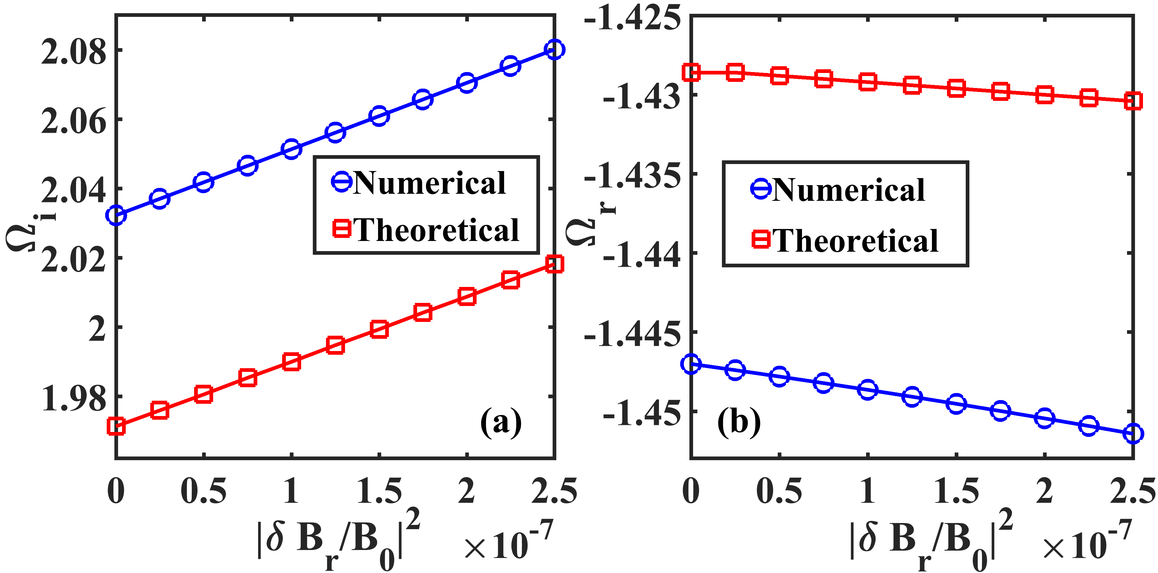
The dependence of ITG growth rate and real frequency on the amplitude of ZS is solved from the theoretical dispersion relation equation (26), which are then compared with the numerical solution of equation (23), as shown in FIG. 1.
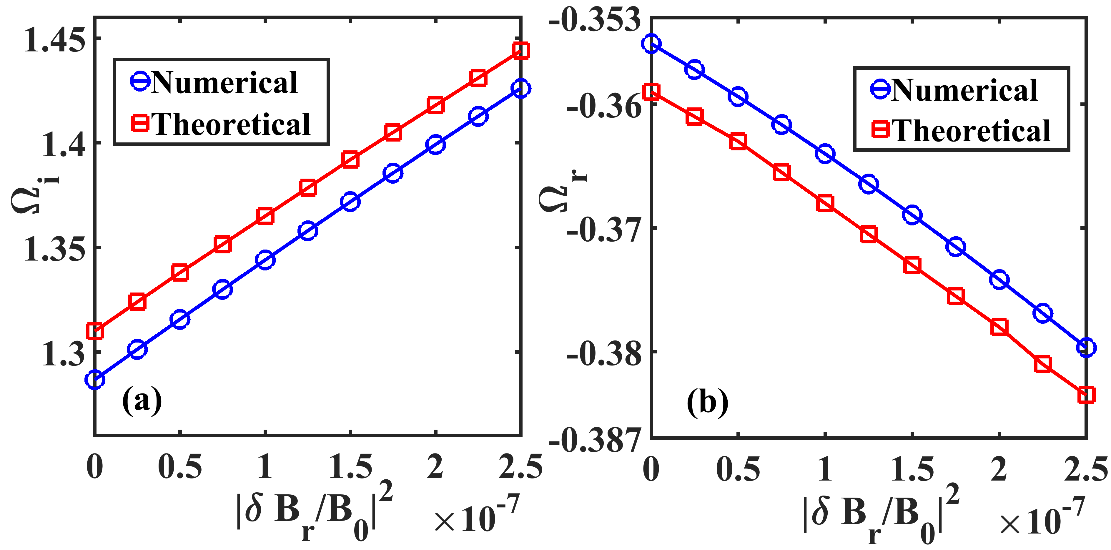
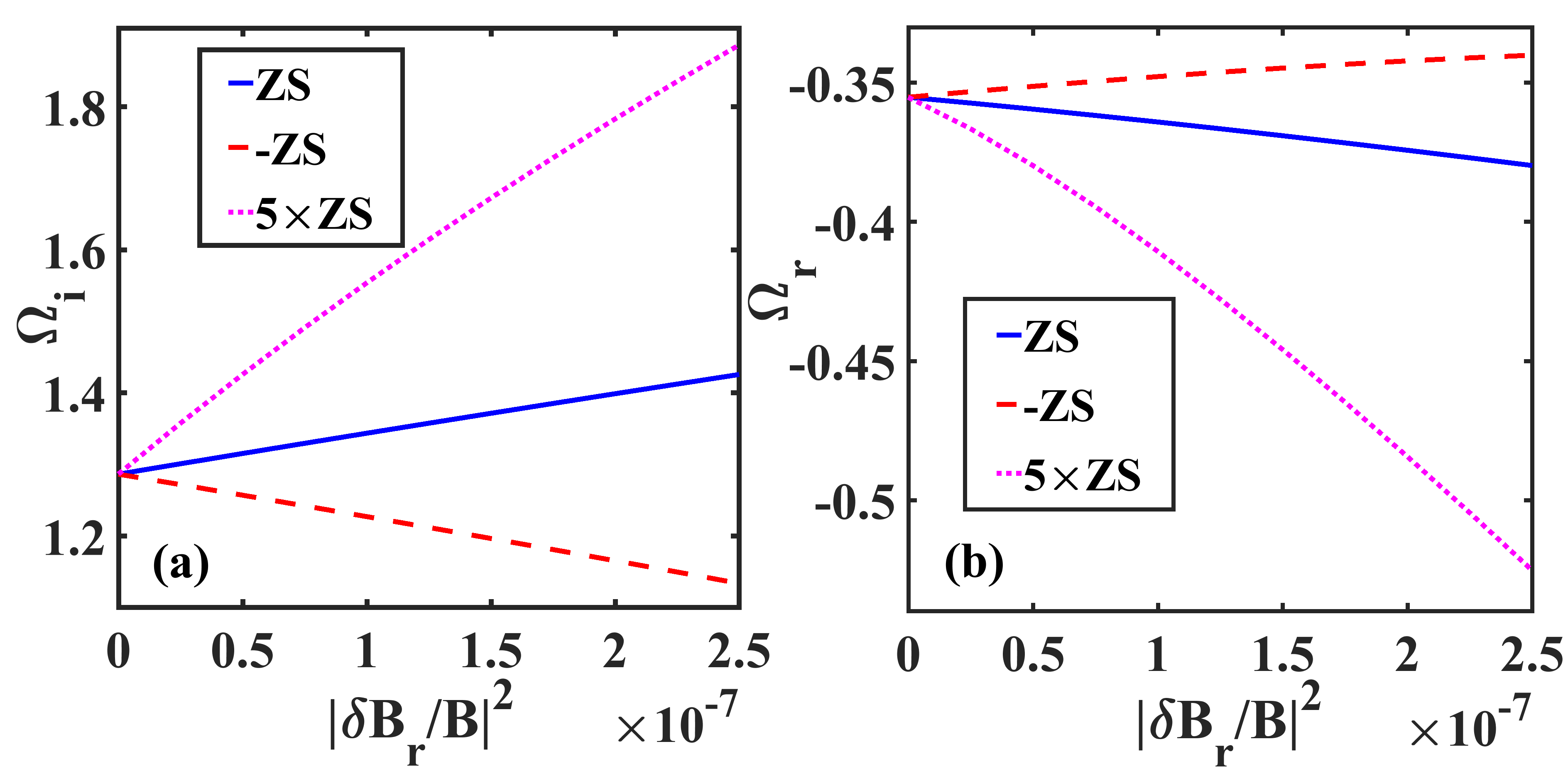
Good agreement between analytical and numerical results are obtained. It is found that, the ITG real frequency as well as growth rate change only slightly with TAE amplitude with the typical tokamak parameters regime, i.e., . More importantly, the ITG growth rate increases with TAE amplitude, suggesting the ZS beat driven by TAE, has only weakly destabilizing effect on ITG stability, contrary to the general speculation. In particular, the influence of ZS on the ITG in our work is significantly less pronounced than the results reported in Ref. 39, where effects of radial electric field from electro-static ZFZF on ITG stability are investigated. This discrepancy primarily stems from the coefficient of the nonlinear term in our equation (23) being substantially smaller than the corresponding coefficient in equation (7) of Ref. 39. In fact, even at the maximum TAE amplitude adopted, the amplitude of the ZS beat-driven by TAE is also quite small, i.e., , so it is reasonable that the impact of the TAE beat-driven ZS on the ITG linear stability is correspondingly weak. If the coefficient of the nonlinear term is artificially enlarged by a factor of five, as depicted by the magenta dotted line in FIG. 2, the destabilizing effect of TAE beat-driven ZS on ITG becomes markedly evident. Besides, in present work, linear growth rate of ITG increase with TAE amplitude, which is in contrast to the numerical results in Ref. 39. The primary reason is attributed to the difference in the sign of the nonlinear terms, which is opposite to that in Ref. 39. As the sign of the nonlinear term in Equation (23) is artificially reversed, as illustrated by the red long dashed line in FIG. 2, the ITG growth rate decreases with TAE amplitude, similar to the results of Ref. 39. However, the underlying physical mechanisms remain elusive and is worthy of further investigation.
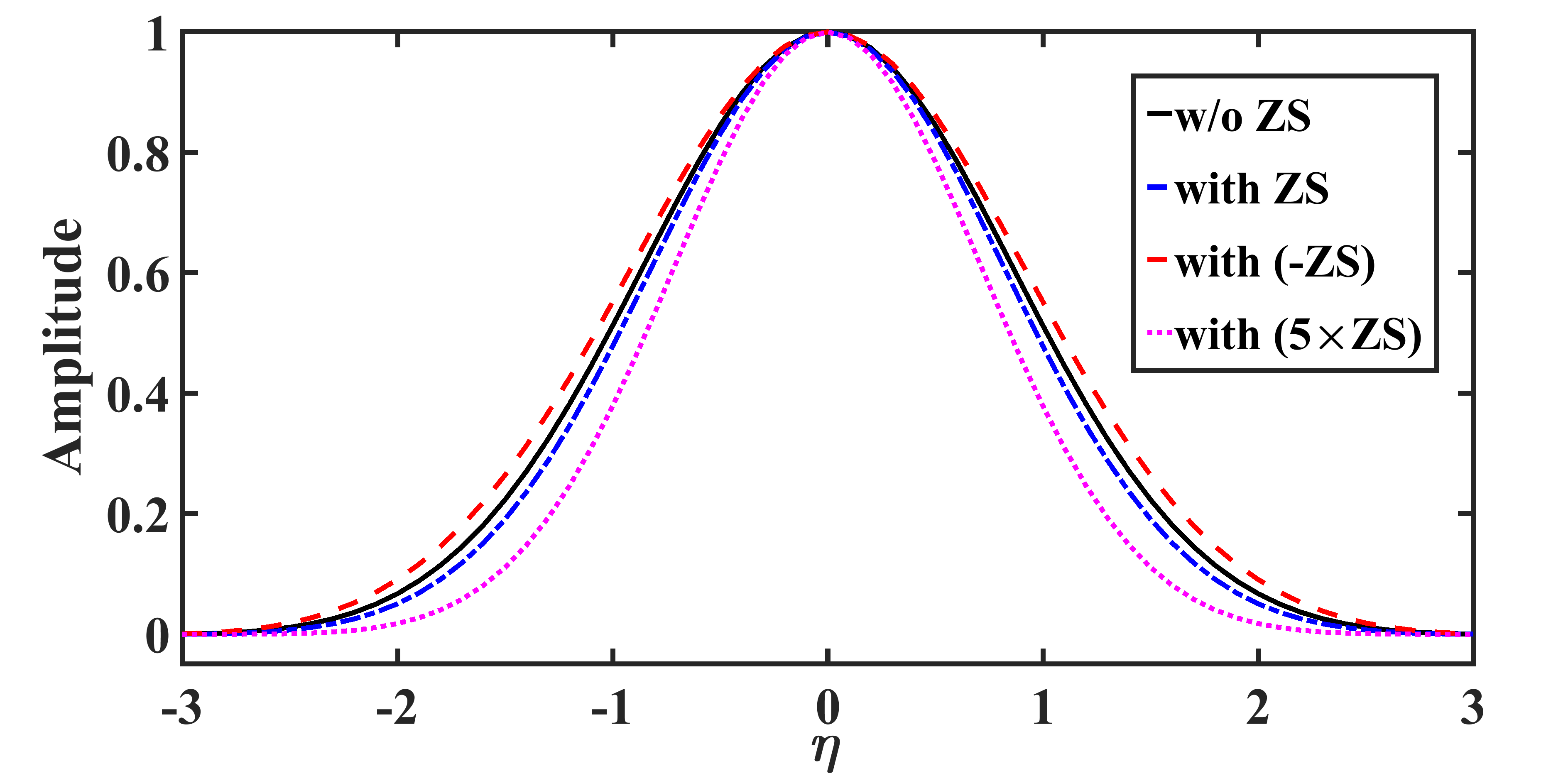
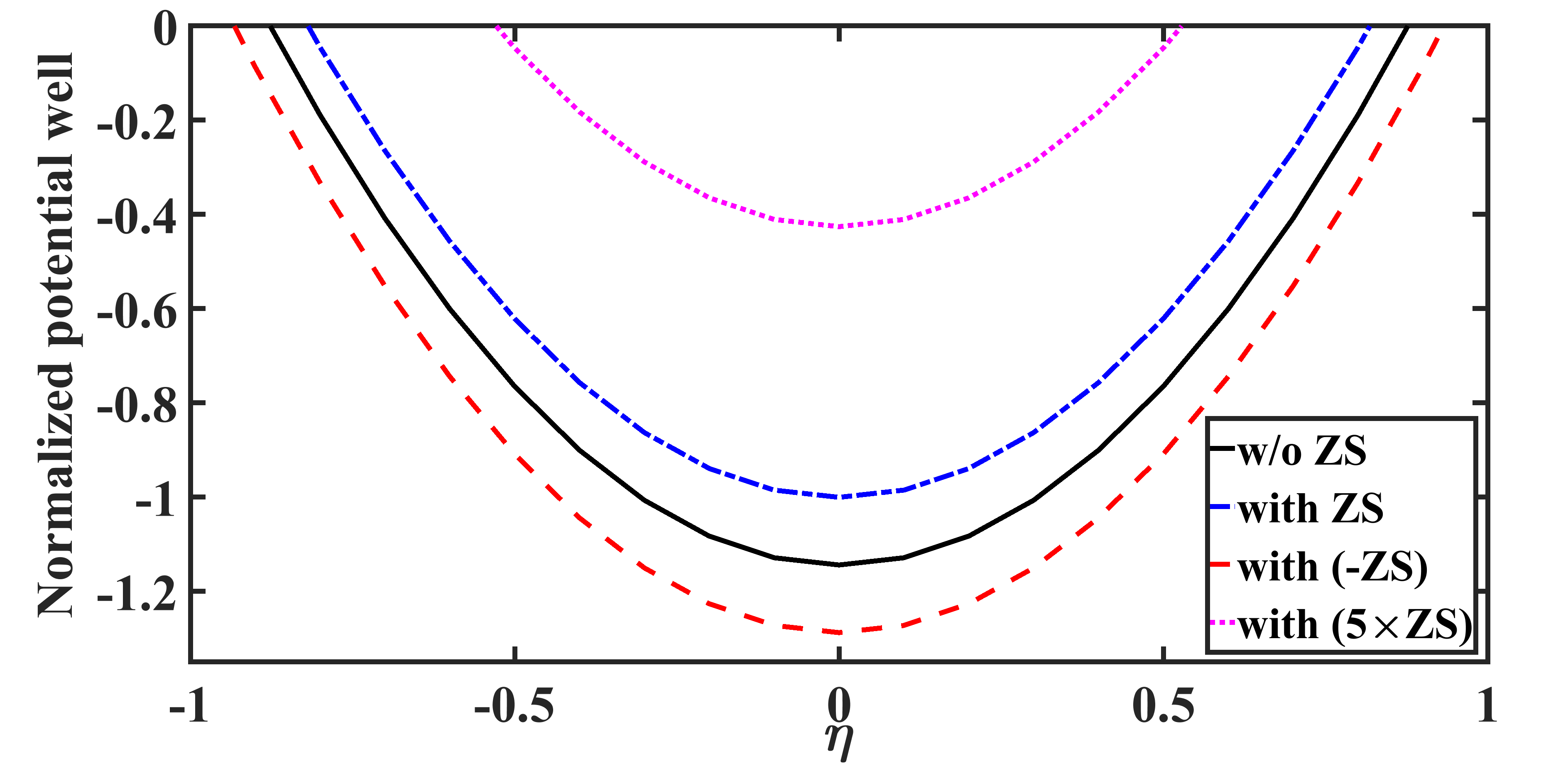
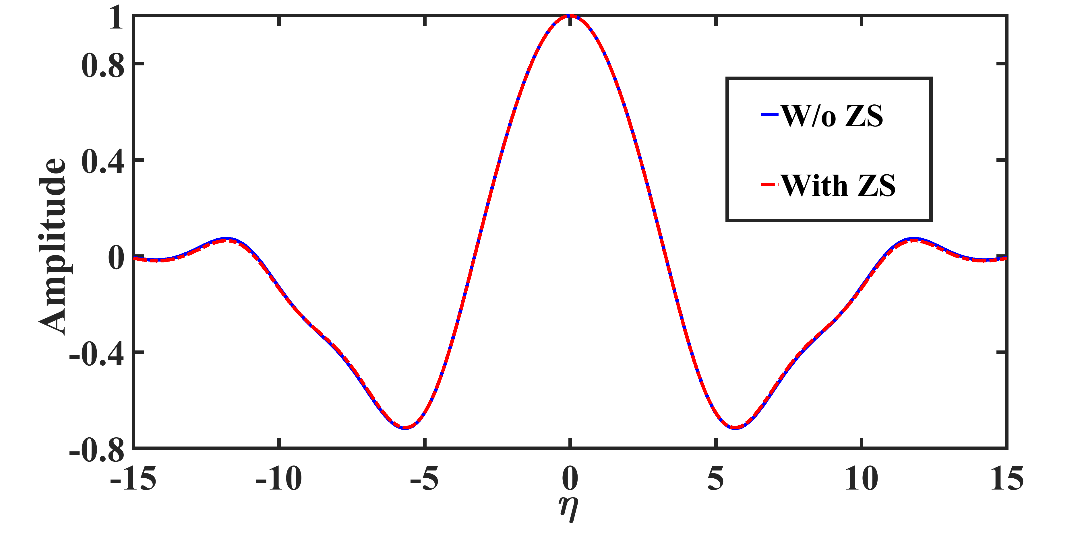
The corresponding mode structures of the most unstable mode are shown in FIG. 3, where the blue dotdash curve represents the case with , red-dashed and magenta dotted curves represent the cases with the nonlinear term artificially changed sign and increased by 5 times, respectively; and the black curve represents the linear mode structure. Clearly, the TAE beat-driven ZS reduces the half-width of the most unstable ITG mode structure. However, even at the maximum amplitude of TAE, the impact of the TAE thermally driven ZS on the ITG mode structure remains minimal. The primary reason is that the TAE beat-driven ZS slightly reduces the depth of the potential well, thereby decreasing the distance between the turning points of the potential well and localizing the ITG mode within a narrower range of stronger drive at the bad curvature region, as shown in FIG. 4, and this is confirmed by the magenta dotted curve and red dashed curve, where the nonlinear term is artificially changed sign or enlarged by a factor. Additionally, the mode structure peaks at and the even symmetry remains unbroken, a result of the even-symmetric modulation introduced by the beat-driven ZS.
V.2 Long-wavelength limit
For typical tokamak plasmas, strong coupling approximation is usually a rough approximation. In more general cases, long wavelength limit with is satisfied Chen, Briguglio, and Romanelli (1991). In the long-wavelength limit, there are two branches, i.e., the toroidal branch and the slab branch. We are more concerned about the toroidal branch Chen, Briguglio, and Romanelli (1991), which is characterized by fast variation over connection length scale () and a superimposed slowly varying envelope over secular scale. Following the analysis of Ref. 46, taking with and denoting slow variation in , the eigenmode equations can be derived from vanishing coefficients of the linearly independent bases and ,
| (27) | |||||
| (28) | |||||
Equation (27) and (28) can be cast into a Weber equation for and , which then yields the dispersion relation for the most unstable ground eigenstate
| (29) | ||||
The dispersion relation is similar to corresponding linear result Chen, Briguglio, and Romanelli (1991), with the term proportional to originating from the contribution of beat-driven ZS.
Following the same procedures, the dependence of the ITG growth rate and real frequency on beat-driven ZS in the long-wavelength limit is illustrated in FIG. 5. Analytical and numerical results indicate that in the long-wavelength limit, the growth rate as well as real frequency of the toroidal branch vary in a similar manner to the results of the short-wavelength limit. That is, the ITG growth rate slightly increases with TAE amplitude, indicating that ZS beat-driven by TAE has only a weakly destabilizing effect on ITG stability due to the relatively small amplitude of the ZS, as well as its phase. The analysis methods are similar to those used in the short-wavelength limit, and thus, will not be repeated here. It is noteworthy that, an artificially small is adopted here to separate different scales for analytical progress, due to the weak dependence of , although this is not the most relevant parameter regime for ITG stability. The mode structure in the long-wavelength limit is presented in FIG. 6, which indicates clearly that the impact of the TAE beat-driven ZS on the most unstable mode is negligible.
VI Summary and discussion
In this work, the indirect nonlinear interaction between toroidal Alfvén eigenmode (TAE) and ion temperature gradient mode (ITG) is investigated using nonlinear gyrokinetic theory and ballooning formalism, to understand the thermal plasma confinement in the presence of energetic particles (EPs) and the associated electromagnetic oscillations. More specifically, the local stability of ITG in the presence of zonal structures (ZS) beat-driven by finite amplitude TAE is analyzed. The governing ITG eigenmode equation in the ballooning space is derived and solved both analytically and numerically, and it is found that, for typical reactor parameters and TAE fluctuation level, the ZS beat-driven by TAE has only weakly destabilizing effects on ITG stability in both short- and long-wavelength limits, contrary to the previous speculations. This is due to the relatively weak ZS generation in the parameter region, i.e., , partly due to the scale separation between TAE and ITG.
In the present analysis, the contributions of zonal field structure, including zonal flow (ZF), zonal current (ZC), and phase space zonal structure (PSZS) are accounted for on the same footing, and only the overall results are analysed. The respective contributions of zonal field structure and PSZS to the ITG dispersion relation in the WKB limit are provided in the Appendix. However, their respective contribution to the ITG stability are not analysed, as the structure of the corresponding eigenmode equation in the ballooning space is significantly modified, due to the non-vanishing nonlinear electron response to ITG, which makes the comparison to the present results not relevant.
The major assumptions made in the present analysis, include 1. the ZS are beat-driven by TAE, and 2. only the local stability of ITG is investigated. It is noteworthy that, in a previous study, it is found that, the direct scattering of electron drift wave (eDW) by finite amplitude ambient TAE has negligible effects on eDW stability Chen, Qiu, and Zonca (2023). The present work, together with Ref. 30, thus, ruled out most channels for the regulation of ITG by ambient electromagnetic oscillations driven by EPs, such as TAE. The potentially effective channels to stabilize DW turbulence, including the spontaneously excited ZS by TAE via modulational instability, as well as DW radial envelope modulation by ZS, are ongoing work of the team, and will be reported in future publications.
Acknowledgement
This work was supported by the Strategic Priority Research Program of Chinese Academy of Sciences under Grant No. XDB0790000, the National Science Foundation of China under Grant Nos. 12275236 and 12261131622, and Italian Ministry for Foreign Affairs and International Cooperation Project under Grant No. CN23GR02. This work was also supported by the EUROfusion Consortium, funded by the European Union via the Euratom Research and Training Programme (Grant Agreement No. 101052200 EUROfusion). The views and opinions expressed are, however, those of the author(s) only and do not necessarily reflect those of the European Union or the European Commission. Neither the European Union nor the European Commission can be held responsible for them.
Appendix A Nonlinear contributions of ZFS and PSZS to ITG
Here, we will give the respective contributions of zonal field structure (ZFS, i.e., and ) and PSZS (i.e., ) on the ITG linear stability. In the nonlinear gyrokinetic equation for nonlinear particle response to ITG
| (30) | ||||
the first and third term in the square bracket on the right hand side are contributions from ZFS (noting that is related to and ), while the second term corresponds to contribution from PSZS.
A.1 Nonlinear contribution of PSZS to ITG
If only PSZS contribution is kept by taking , , it results in , the corresponding nonlinear particle response to ITG can be derived as
| (31) | |||||
| (32) |
Substituting equations (31) and (32) into the quasi-neutrality condition, the nonlinear ITG equation in the presence of PSZS beat-driven by TAE can be derived as
| (33) | ||||
with the term proportional to being the contribution of PSZS beat-driven by TAE.
A.2 Nonlinear contribution of ZFS to ITG
If we consider only the ZFS contribution by taking , one then obtains the nonlinear particle response to ITG as
| (34) | |||||
| (35) |
Substituting equations (34) and (35) into the quasi-neutrality condition, the nonlinear ITG equation can be derived as
| (36) | ||||
Equation (22) can be recovered by combining the nonlinear terms of equations (33) and (36), i.e., the contributions of PSZS and ZFS. We however, will not compare the results of equations (33) and (36) to that of equation (22), as the structures of the equations are very different. More specifically, the terms in equations (33) and (36) due to non-vanishing nonlinear electron response to ITG, render the corresponding ITG eigenmode equations into a third order differential equation in ballooning space, whereas equation (22) will yield a second order differential equation in ballooning space, as the terms proportional to in equations (33) and (36) cancel each other.
References
- Horton (1999) W. Horton, Rev. Mod. Phys. 71, 735 (1999).
- Kolesnichenko (1967) Y. I. Kolesnichenko, At. Energ 23, 289 (1967).
- Mikhailovskii (1975) A. Mikhailovskii, Zh. Eksp. Teor. Fiz 68, 25 (1975).
- Rosenbluth and Rutherford (1975) M. Rosenbluth and P. Rutherford, Phys. Rev. Lett. 34, 1428 (1975).
- Chen (1994) L. Chen, Physics of Plasmas 1, 1519 (1994).
- Fasoli et al. (2007) A. Fasoli, C. Gormenzano, H. Berk, B. Breizman, S. Briguglio, D. Darrow, N. Gorelenkov, W. Heidbrink, A. Jaun, S. Konovalov, R. Nazikian, J.-M. Noterdaeme, S. Sharapov, K. Shinohara, D. Testa, K. Tobita, Y. Todo, G. Vlad, and F. Zonca, Nuclear Fusion 47, S264 (2007).
- Chen and Zonca (2016) L. Chen and F. Zonca, Review of Modern Physics 88, 015008 (2016).
- Zonca et al. (2015a) F. Zonca, L. Chen, S. Briguglio, G. Fogaccia, A. V. Milovanov, Z. Qiu, G. Vlad, and X. Wang, Plasma Physics and Controlled Fusion 57, 014024 (2015a).
- Nazikian et al. (2008) R. Nazikian, G. Y. Fu, M. E. Austin, H. L. Berk, R. V. Budny, N. N. Gorelenkov, W. W. Heidbrink, C. T. Holcomb, G. J. Kramer, G. R. McKee, M. A. Makowski, W. M. Solomon, M. Shafer, E. J. Strait, and M. A. V. Zeeland, Phys. Rev. Lett. 101, 185001 (2008).
- Qiu, Chen, and Zonca (2016a) Z. Qiu, L. Chen, and F. Zonca, Nuclear Fusion 56, 106013 (2016a).
- Qiu, Chen, and Zonca (2017) Z. Qiu, L. Chen, and F. Zonca, Nuclear Fusion 57, 056017 (2017).
- Falessi et al. (2023) M. Falessi, L. Chen, Z. Qiu, and F. Zonca, to be submitted to New Journal of Physics (2023).
- Zonca et al. (2021) F. Zonca, L. Chen, M. Falessi, and Z. Qiu, Journal of Physics: Conference Series 1785, 012005 (2021).
- Di Siena et al. (2021) A. Di Siena, R. Bilato, T. Görler, A. B. Navarro, E. Poli, V. Bobkov, D. Jarema, E. Fable, C. Angioni, Y. O. Kazakov, et al., Physical Review Letters 127, 025002 (2021).
- Han et al. (2022) H. Han, S. Park, C. Sung, J. Kang, Y. Lee, J. Chung, T. S. Hahm, B. Kim, J.-K. Park, J. Bak, et al., Nature 609, 269 (2022).
- Romanelli et al. (2010) M. Romanelli, A. Zocco, F. Crisanti, J.-E. Contributors, et al., Plasma Physics and Controlled Fusion 52, 045007 (2010).
- Tardini et al. (2007) G. Tardini, J. Hobirk, V. Igochine, C. Maggi, P. Martin, D. McCune, A. Peeters, A. Sips, A. Stäbler, J. Stober, and the ASDEX Upgrade Team, Nuclear Fusion 47, 280 (2007).
- Bourdelle et al. (2005) C. Bourdelle, G. Hoang, X. Litaudon, C. Roach, and T. Tala, Nuclear fusion 45, 110 (2005).
- Di Siena et al. (2018) A. Di Siena, T. Görler, H. Doerk, E. Poli, and R. Bilato, Nuclear Fusion 58, 054002 (2018).
- Bonanomi et al. (2018) N. Bonanomi, P. Mantica, A. D. Siena, E. Delabie, C. Giroud, T. Johnson, E. Lerche, S. Menmuir, M. Tsalas, D. V. Eester, and J. Contributors, Nuclear Fusion 58, 056025 (2018).
- Citrin et al. (2014) J. Citrin, J. Garcia, T. Görler, F. Jenko, P. Mantica, D. Told, C. Bourdelle, D. Hatch, G. Hogeweij, T. Johnson, et al., Plasma Physics and Controlled Fusion 57, 014032 (2014).
- Citrin and Mantica (2023) J. Citrin and P. Mantica, Plasma Physics and Controlled Fusion 65, 033001 (2023).
- Citrin et al. (2013) J. Citrin, F. Jenko, P. Mantica, D. Told, C. Bourdelle, J. Garcia, J. W. Haverkort, G. M. D. Hogeweij, T. Johnson, and M. J. Pueschel, Phys. Rev. Lett. 111, 155001 (2013).
- Marchenko (2022) V. Marchenko, Physics of Plasmas 29, 030702 (2022).
- Cheng, Chen, and Chance (1985) C. Cheng, L. Chen, and M. Chance, Ann. Phys. 161, 21 (1985).
- Hasegawa, Maclennan, and Kodama (1979) A. Hasegawa, C. G. Maclennan, and Y. Kodama, Physics of Fluids 22, 2122 (1979).
- Rosenbluth and Hinton (1998) M. N. Rosenbluth and F. L. Hinton, Phys. Rev. Lett. 80, 724 (1998).
- Mazzi et al. (2022) S. Mazzi, J. Garcia, D. Zarzoso, Y. O. Kazakov, J. Ongena, M. Dreval, M. Nocente, Ž. Štancar, G. Szepesi, J. Eriksson, et al., Nature Physics 18, 776 (2022).
- Chen, Qiu, and Zonca (2022) L. Chen, Z. Qiu, and F. Zonca, Nuclear Fusion 62, 094001 (2022).
- Chen, Qiu, and Zonca (2023) L. Chen, Z. Qiu, and F. Zonca, Nuclear Fusion 63, 106016 (2023).
- Chen and Zonca (2012) L. Chen and F. Zonca, Phys. Rev. Lett. 109, 145002 (2012).
- Zonca et al. (2015b) F. Zonca, L. Chen, S. Briguglio, G. Fogaccia, G. Vlad, and X. Wang, New Journal of Physics 17, 013052 (2015b).
- Chen, Lin, and White (2000) L. Chen, Z. Lin, and R. White, Physics of Plasmas 7, 3129 (2000).
- Lin et al. (1998) Z. Lin, T. S. Hahm, W. W. Lee, W. M. Tang, and R. B. White, Science 281, 1835 (1998).
- Todo, Berk, and Breizman (2010) Y. Todo, H. Berk, and B. Breizman, Nuclear Fusion 50, 084016 (2010).
- Biancalani et al. (2020) A. Biancalani, A. Bottino, P. Lauber, A. Mishchenko, and F. Vannini, Journal of Plasma Physics 86, 825860301 (2020).
- Qiu, Chen, and Zonca (2016b) Z. Qiu, L. Chen, and F. Zonca, Physics of Plasmas (1994-present) 23, 090702 (2016b).
- Chen et al. (2023) L. Chen, Z. Qiu, F. Zonca, M. V. Falessi, P. Liu, and R. Ma, in The 14th International West Lake Symposium- Frontier Progress in Fusion Energy Research and Development (2023).
- Chen et al. (2021) N. Chen, H. Hu, X. Zhang, S. Wei, and Z. Qiu, Physics of Plasmas 28, 042505 (2021).
- Frieman and Chen (1982) E. A. Frieman and L. Chen, Physics of Fluids 25, 502 (1982).
- Connor, Hastie, and Taylor (1978) J. Connor, R. Hastie, and J. Taylor, Phys. Rev. Lett. 40, 396 (1978).
- Wang et al. (2020) H. Y. Wang, I. Holod, Z. Lin, J. Bao, J. Y. Fu, P. F. Liu, J. H. Nicolau, D. Spong, and Y. Xiao, Physics of Plasmas 27, 082305 (2020).
- Dong et al. (2019) G. Dong, J. Bao, A. Bhattacharjee, and Z. Lin, Physics of Plasmas 26 (2019).
- Cheng and Chen (1980) C. Z. Cheng and L. Chen, The Physics of Fluids 23 (1980).
- Guzdar et al. (1983) P. N. Guzdar, L. Chen, W. M. Tang, and P. H. Rutherford, The Physics of Fluids 26, 673 (1983).
- Chen, Briguglio, and Romanelli (1991) L. Chen, S. Briguglio, and F. Romanelli, Physics of Fluids B: Plasma Physics 3, 611 (1991).
- Heidbrink et al. (2007) W. W. Heidbrink, N. N. Gorelenkov, Y. Luo, M. A. Van Zeeland, R. B. White, M. E. Austin, K. H. Burrell, G. J. Kramer, M. A. Makowski, G. R. McKee, and R. Nazikian (the DIII-D team), Phys. Rev. Lett. 99, 245002 (2007).