A Neural Material Point Method
for Particle-based Simulations

Abstract

Mesh-free Lagrangian methods are widely used for simulating fluids, solids, and their complex interactions due to their ability to handle large deformations and topological changes. These physics simulators, however, require substantial computational resources for accurate simulations. To address these issues, deep learning emulators promise faster and scalable simulations, yet they often remain expensive and difficult to train, limiting their practical use. Inspired by the Material Point Method (MPM), we present NeuralMPM, a neural emulation framework for particle-based simulations. NeuralMPM interpolates Lagrangian particles onto a fixed-size grid, computes updates on grid nodes using image-to-image neural networks, and interpolates back to the particles. Similarly to MPM, NeuralMPM benefits from the regular voxelized representation to simplify the computation of the state dynamics, while avoiding the drawbacks of mesh-based Eulerian methods. We demonstrate the advantages of NeuralMPM on several datasets, including fluid dynamics and fluid-solid interactions. Compared to existing methods, NeuralMPM reduces training times from days to hours, while achieving comparable or superior long-term accuracy, making it a promising approach for practical forward and inverse problems. A project page is available at https://neuralmpm.isach.be

1 Introduction

The Navier-Stokes equations describe the time evolution of fluids and their interactions with solid materials. As analytical solutions rarely exist, numerical methods are required to approximate the solutions. These methods can be broadly categorized into Eulerian and Lagrangian approaches, each with its own strengths and weaknesses. On the one hand, Eulerian methods discretize the fluid domain on a fixed grid, simplifying the computation of the dynamics, but requiring high-resolution meshes to solve small-scale details in the flow. Lagrangian methods, on the other hand, represent the fluid as virtual moving particles defining the system’s state, hence maintaining a high level of detail in regions of high density. While effective at handling deformations and topological changes [1], Lagrangian methods struggle with collisions and interactions with rigid objects [2, 3].

Regardless of the discretization strategy, large-scale high-resolution numerical simulations are computationally expensive, limiting their practical use in downstream tasks such as forecasting, inverse problems, or computational design. To address these issues, deep learning emulators have shown promise in accelerating simulations by learning an emulator model that can predict the system’s state at a fraction of the cost. Next to their speed, neural emulators also have the strategic advantage of being differentiable, enabling their use in inverse problems and optimization tasks [4, 5, 6, 7, 8, 9]. Moreover, they have the potential to be learned directly from real data, bypassing the costly and resource-intensive process of building a simulator [10, 11, 12, 13, 14, 15, 16, 17]. In this direction, particle-based neural emulators [18, 19, 20] have seen success in accurately simulating fluids and generalizing to unseen environments. These emulators, however, suffer from the same issues as traditional Lagrangian methods, with collisions and interactions with rigid objects being particularly challenging. These emulators may also require long training and inference times, limiting their practical use.

Taking inspiration from the hybrid Material Point Method (MPM) [21, 22] that combines the strengths of both Eulerian and Lagrangian methods, we introduce NeuralMPM, a neural emulation framework for particle-based simulations. As in MPM, NeuralMPM maintains Lagrangian particles to represent the system’s state but models the system dynamics on voxelized representations. In this way, NeuralMPM benefits from a regular grid structure to simplify the computation of the state dynamics but avoids the drawbacks of mesh-based Eulerian methods. By interpolating the particles onto a fixed-size grid, it also bypasses the need to perform an expensive neighbor search at every timestep, substituting it with two interpolation steps based on cheap voxelization [23, 24, 20]. Furthermore, by defining the system dynamics on a grid, NeuralMPM can leverage well-established grid-to-grid neural network architectures. The resulting inductive bias allows the model to more easily process the global and local structures of the point cloud, instead of having to discover them, and frees capacity for learning the dynamics of the system represented by the grid. Compared to previous data-driven approaches [18, 19, 20], these improvements reduce the training time from days to hours, while achieving higher or comparable accuracy.

2 Computational Fluid Dynamics

Computational fluid dynamics simulations can be classified into two broad categories, Eulerian and Lagrangian, depending on how the discretization of the continuous fluid is handled [25]. In Eulerian simulations, the domain is discretized with a mesh, with state variables $u^{t}_{i}$ (such as mass or momentum) maintained at each mesh point $i$. Well-known examples of Eulerian simulations are the finite difference method, where the domain is divided into a uniform regular grid (also called an Eulerian grid), and the finite element method, where the domain is divided into regions, or elements, that may have different shapes and density, allowing to increase the resolution in only some areas of the domain [26, 27]. Lagrangian simulations, on the other hand, discretize the fluid as a set of virtual moving particles $\{p^{t}_{i},u^{t}_{i}\}_{i=1}^{N}$, each described by its position $p^{t}_{i}$ and state variables $u^{t}_{i}$ that include the particle velocity $v^{t}_{i}$. To simulate the fluid, the particles move according to the dynamics of the system, producing a new set of particles $\{p^{t+1}_{i},u^{t+1}_{i}\}_{i=1}^{N}$ at each timestep. Simulations in Lagrangian coordinates are particularly useful when the fluid is highly deformable, as the particles can move freely and adapt to the fluid’s shape. Among Lagrangian methods, Smoothed Particle Hydrodynamics (SPH) is one of the most popular, where the fluid is represented by a set of particles that interact with each other through a kernel function that smooths the interactions. SPH has been widely used in large-scale astrophysical simulations, such as galactic dynamics [28, 29] or planetary collision [30], and in ocean engineering [31, 32, 33] to model deformations and fractures.

Hybrid Eulerian-Lagrangian methods combine the strengths of both frameworks. Like Lagrangian methods, they carry the system state information via particles, thereby automatically adjusting the resolution to the local density of the system. By using a regular grid, however, they simplify gradient computation, make entity contact detection easier, and prevent cracks from propagating only along the mesh. Among hybrid methods, the Material Point Method has gained popularity for its ability to handle large deformations and topological changes. MPM combines a regular Eulerian grid with moving Lagrangian particles. It does so in four main steps: (1) the quantities carried by the particles are interpolated onto a regular grid $G^{t}=\textbf{p2g}(\{p^{t}_{i},u^{t}_{i}\})$ using a particle-to-grid (p2g) function, (2) the equations of motion are solved on the grid, where derivatives and other quantities are easier to compute, resulting in a new grid state $G^{t+1}=f(G^{t})$, (3) the resulting dynamics are interpolated back onto the particles as $\{u^{t+1}_{i}\}=\textbf{g2p}(G^{t+1},\{p^{t}_{i}\})$, using a grid-to-particle (g2p) function, (4) the positions of the particles are updated by computing particle-wise velocities and using an appropriate integrator, such as Euler, i.e., $p^{t+1}_{i}=p^{t}_{i}+\Delta tv^{t+1}_{i}$. The grid values are then reset for the next step. MPM has been used in soft tissue simulations [34], in molecular dynamics [35], in astrophysics [36], in fluid-membrane interactions [37], and in simulating cracks [38] and landslides [39]. MPM is also widely used in the animation industry, perhaps most notably in Disney’s 2013 film Frozen [40], where it was used to simulate snow.

Notwithstanding the success of numerical simulators, they remain expensive, slow, and, most of the time, non-differentiable. In recent years, differentiable neural emulators have shown great promise in accelerating fluid simulations, most notably in a series of works to emulate SPH simulations in a fully data-driven manner. Graph network-based simulators (GNS) [18] use a graph neural network (GNN) and a graph built from the local neighborhood of the particles to predict the acceleration of the system. The approach requires building a graph out of the point cloud at every timestep to obtain structural information about the cloud, which is an expensive operation. In addition, the GNN needs to extract global information from its nodes, which is only possible with a high number of message-passing steps, resulting in a large computational graph and long training and inference times. This large computational graph, along with repeated construction, makes fully autoregressive training over long rollouts impractical, as the gradients need to backpropagate all the way back to the first step. Cheaper strategies exist, like the push-forward trick [41], but they have been shown to be inferior to fully backpropagating through trajectories [42, 43]. As autoregressive training is not available, the stability of the learned dynamics can be compromised, making the model prone to diverging or oscillating. Noise injection training strategies can be used to increase the stability of the rollouts, but the magnitude of the noise becomes a critical parameter. Han et al. [44] introduce improvements to GNS to make them subequivariant to certain transformations. They show increased accuracy on simulations involving solid objects. An alternative approach is the continuous convolution (CConv) [19], an extension of convolutional networks to point clouds. In this method, a convolutional kernel is applied to each particle by interpolating the values of the kernel at the positions of its neighbors, which are found via spatial hashing on GPU, a cheaper alternative to tree-based searches that allows for autoregressive training. In [20], Deep Momentum Conserving Fluids (DMCF) build upon CConv to design a momentum-conserving architecture. Nevertheless, to account for long-range interactions, the authors introduce different branches, with different receptive fields, into their network. The number of branches, and their hyperparameters, need to be tuned to capture global dependencies, leading to long training times even with optimized CUDA kernels. Finally, Zhang et al. [45], propose an approach that uses nearest neighbors to construct the local features of each particle. Those local features are then averaged onto a regular grid. Like GNS, this method suffers from the need to repeat the neighbor search at every simulation timestep. Ultimately, the performance of point cloud-based simulators is tightly linked to the method used to process the spatial structure of the cloud. Brute force neighbour search is $\mathcal{O}(N^{2})$, K-d trees are $\mathcal{O}(N\log{N})$, and voxelization and hashing are $\mathcal{O}(N)$ [24, 46].

An alternative to data-driven modeling is the use of hybrid models. In hybrid ML models, part of a classical solver is replaced with a learned component. For instance, Yin et al. [47] employ a neural network to learn unknown physics, which is then integrated into a simulator. Similarly, Li et al. [48] use a neural network to bypass computational bottlenecks in MPM simulators, while Ma et al. [49] learn general constitutive laws, allowing for one-shot trajectory learning. These approaches achieve impressive results by leveraging extensive physics knowledge, but this reliance also limits their applicability. Hybrid models inherit both the strengths and weaknesses of classical and ML methods.

3 NeuralMPM

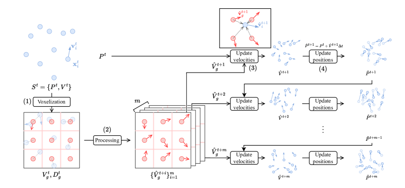
Figure 1: NeuralMPM works in 4 steps. (1) The positions $P^{t}$ and velocities $V^{t}$ of the particles are used to compute the velocity $V^{t}_{g}$ and density $D^{t}_{g}$ of each grid node through voxelization. (2) From this grid, the processor neural network predicts the grid velocities at the next $m$ timesteps. The next $m$ positions are computed iteratively by (3) performing bilinear interpolation of the predicted velocities onto the previous positions and (4) updating the positions using the predicted velocities.

We consider a Lagrangian system evolving in time and defined by the positions $p^{t}_{i}$ and velocities $v^{t}_{i}$ of a set of $N$ particles $i=1,...,N$. For notational simplicity, we denote with $P^{t}$ and $V^{t}$ the set of positions and velocities of all particles at time $t$ and with $S^{t}=(P^{t},V^{t})$ the full state of the system. In a more complex setting, the state of the system can include other local properties, such as pressure or elastic stiffness of materials, and global properties, such as an external force. In this work, for simplicity, we let the network learn the relevant simulation parameters implicitly. The evolution of the particles is described by a function $f$ mapping the current state of the system to its next state $S^{t+1}=f(S^{t})$. Given a starting system $S^{0}=(P^{0},V^{0})$, its full trajectory, or rollout, is denoted by $S^{1:T}$. Our goal is to build an emulator $\hat{f}_{\theta}(\cdot)$ capable of predicting a full rollout $\hat{f}_{\theta}^{1:T}(S^{0})$ of $T$ timesteps from the initial state $S^{0}$. Following MPM, NeuralMPM operates in four steps, as illustrated in Figure 1:

Step 1: Voxelization.

Using the positions $P^{t}$, the velocities $V^{t}$ of the particles in the point cloud are interpolated onto a regular fixed-size grid. This interpolation is performed through voxelization, which divides the domain into regular volumes (voxels). Each grid node is identified as the center of a voxel (e.g., square in 2D) in the domain, and the velocities of the particles in the voxel are averaged to give the node’s velocity. Similarly, the density is computed as the normalized number of particles in the voxel. This results in the grid tensor $G^{t}$ that contains the grid velocities $V^{t}_{g}$ and density $D^{t}_{g}$.

Step 2: Processing.

Taking advantage of the regular grid representation of the cloud, the grid velocities $\{\hat{V}^{i}\}_{i=t+1}^{t+m}$ of the next $m$ timesteps are predicted using a neural network. We chose a U-Net [50] as it is a well-established image-to-image model, known to perform well in various tasks, including physical applications. The combination of kernels applied with different receptive fields (from smaller to larger) allows the U-Net to efficiently extract both local and global information. Nonetheless, any grid-to-grid architecture could be used. We experiment with the FNO [51] architecture in Appendix B and find it to underperform, leading us to keep the U-Net. A fully convolutional U-Net and an FNO have the additional advantage of being able to generalize to different domain shapes, a desirable property (Section 4.3).

Step 3: Update of particle velocities.

The predicted velocities $\hat{V}^{t+1}$ at the next timestep are then interpolated back to the particle level onto the positions $P^{t}$ using bilinear interpolation. The velocity of each particle is computed as a weighted average of the four surrounding grid velocities, based on its Euclidean distance to each of them.

Step 4: Update of particle positions.

Finally, the positions of the particles are updated with Euler integration using the next velocities and known current positions of the particles, that is $\hat{P}^{t+1}=P^{t}+\Delta t\hat{V}^{t+1}$. Steps 3 and 4 are performed $m$ times to compute the next $m$ positions from the set of grid velocities computed at step 2.

Additional features of the individual particles can be included in the grid tensor $G^{t}$ by interpolating them in the same way as the velocities. Local, such as boundary conditions, or global, such as gravity or external forces, features are represented as grid channels. For simulations with multiple types of particles, the velocity and density of each material are interpolated independently and stacked as channels in the grid tensor $G_{t}$.

NeuralMPM is trained end-to-end on a set of trajectories $S^{0:T}$ to minimize the mean squared error $||P^{t+1}-\hat{P}_{\theta}^{t+1}(S^{t})||^{2}_{2}$ between the ground-truth and predicted next positions of the particles. At inference time, the model is exposed to much longer sequences, which requires carefully stabilizing the rollout procedure to prevent the accumulation of large errors over time. To address this, we first make use of autoregressive training [20, 19], where the model is unrolled $K$ times on its own predictions, producing a sequence of $\hat{S}^{k}=\hat{f}_{\theta}(\hat{S}^{k-1})$ for $k=1,...,K$ and initial input $\hat{S}^{0}=S^{0}$, before backpropagating the error through the entire rollout. Unlike more costly methods that require alternative stabilization strategies, such as noise injection [18], NeuralMPM’s efficiency makes autoregressive training possible. Nevertheless, to further stabilize the training, we couple autoregressive training with time bundling [41], resulting in a training strategy where the model predicts $m$ steps $\hat{S}^{1:m}$ at once from a single initial state, inside an outer autoregressive loop of $K$ steps of length $m$. We show in Section 4 that this training strategy leads to more accurate rollouts.

4 Experiments

We conduct a set of diverse experiments to demonstrate the accuracy, speed, and generalization capabilities of NeuralMPM. Specifically, we examine its robustness to hyperparameter and architectural choices through an ablation study (4.1). We compare NeuralMPM to GNS [18] and DMCF [20] in terms of accuracy, training time, convergence, and inference speed (4.2). We also evaluate the generalization capabilities of NeuralMPM (4.3) and illustrate how its differentiability can be leveraged to solve an inverse design problem (4.4). Through these experiments, we demonstrate that NeuralMPM is a flexible, accurate, and fast method for emulating complex particle-based simulations.

Data.

We consider 6 datasets with variable sequence lengths, numbers of particles, and materials. The first three datasets, WaterRamps, SandRamps, and Goop, contain a single material, water, sand, and goop, respectively, with different material properties. The first two datasets contain random ramp obstacles to challenge the model’s generalization capacity. The fourth dataset, MultiMaterial, mixes the three materials together in the same simulations. These four datasets are taken from [18] and were simulated using the Taichi-MPM simulator [52]. They each contain 1000 trajectories for training and 30 (Goop) or 100 (WaterRamps, SandRamps, MultiMaterial) for validation and testing. The fifth dataset, WBC-SPH [20], was generated using a high-fidelity SPH solver [53] and contains water, random obstacles, and variable gravity. It contains 30 trajectories for training and 9 for validation and testing. The last dataset, Dam Break 2D, was also generated using SPH and contains 50 trajectories for learning, and 25 for validation and testing. Rollout snapshots of NeuralMPM compared to the ground truth for each dataset are shown in Figure 2.

Protocol.

NeuralMPM is trained on a set of full trajectories, with varying initial conditions and number of particles. The training batches are sampled randomly in time and across sequences. We use the Adam optimizer [54] with the following learning rate schedule: a linear warm-up over 100 steps from $10^{-5}$ to $10^{-3}$, $900$ steps at $10^{-3}$, then a cosine annealing [55] for $100,000$ iterations. We use a batch size of $128$, $K=4$ autoregressive steps per iteration, bundle $m=8$ timesteps per model call (resulting in $24$ predicted states), and a grid size of $64\times 64$. For most of our experiments, we use a U-Net [50] with three downsampling blocks with a factor of $2$, $64$ hidden channels, a kernel size of $3$, and MLPs with three hidden layers of size $6$4 for pixel-wise encoding and decoding into a latent space. For a fair comparison, we ran training and inference for NeuralMPM, DMCF, and GNS on the exact same hardware. GNS and DMCF were trained until convergence (a maximum of 120 and 240 hours, respectively), while NeuralMPM required 20 hours or less to converge. Further details on training can be found in Appendix A.

	WaterRamps	SandRamps	Goop	MultiMaterial	WBC-SPH	Dam Break 2D
Initial
Predictions
Ground Truth

Figure 2: Example snapshots. We train and evaluate NeuralMPM on WaterRamps, SandRamps and Goop, each consisting of a single material, on MultiMaterial that mixes water, sand and goop, on WBC-SPH with more complex obstacles and variable gravity, and on Dam Break 2D, a rectangular-shaped SPH dataset. NeuralMPM is able to learn various kinds of materials, their interactions, and their interactions with solid obstacles. Despite being inspired by MPM, it is not limited to data showing MPM-like behaviour.

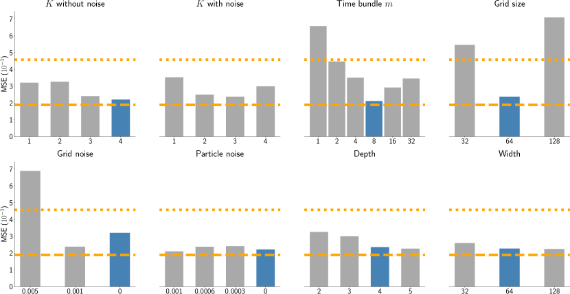
Figure 3: Ablation results. Mean squared error (MSE) of full rollouts on unseen test data for Goop. The default parameters are in blue. The dashed orange line shows the best rollout MSE of GNS as reported in [18] on the same data ($1.89\times 10^{-3}$), while the dotted line ($2.4\times 10^{-3}$) indicates the MSE we obtained for GNS after $240$ hours ($20$M training steps). NeuralMPM is robust to hyperparameter changes, with the biggest effects coming from the number of timesteps bundled together ($m$) and grid noise. For a rollout of length $T$, the model is called $T/m$ times, meaning lower values of $m$ require maintaining stability for longer. Autoregressive training coupled with time bundling is sufficient to stabilize the model, eliminating the need for noise injection. Although GNS reportedly outperforms NeuralMPM by a small margin, these results could not be reproduced in our experiments.

4.1 Ablation study

To study the robustness of NeuralMPM to hyperparameter and architectural choices, we start with the default architecture and hyperparameters and ablate its components individually to examine their impact on performance. We vary the number $K$ of autoregressive steps with and without noise, the number of bundled timesteps $m$ predicted by a single model call, and the depth and number of hidden channels of the network. We also investigate adding noise to stabilize rollouts, either directly to the particles’ positions or to the grid-level representation after voxelization.

Figure 3 summarizes the ablation results. A larger number $K$ of autoregressive steps yields more accurate rollouts without the need to add noise. Indeed, injecting noise does not improve accuracy and is even detrimental for $K=4$. Individually tuning the noise levels for grids and particles can modestly lower error rates, but is either very sensitive or negligible. The model performs better when bundling more timesteps, enabling faster rollouts as a single forward pass predicts more steps. We found $m=8$ to be optimal with the other default hyperparameters, outperforming larger bundling. This is because more network capacity is needed to extract information for the next $16$ or $32$ timesteps from a single state. Instead, we opted for a shallower and narrower network to balance speed and memory footprint with performance gains. In terms of network architecture, we chose a U-Net. We experiment with an FNO [51] in Appendix B and find it to underperform, leading us to keep the U-Net architecture. We find the U-Net’s width and depth to have a minor impact on performance, confirming that a larger network is not needed. The grid size, however, is critical. A low resolution loses fine details, while a high resolution turns meaningful structures, such as liquid blobs or walls, into isolated voxels.

Given these results, we conduct the rest of our experiments using the blue parameters in Figure 3, except for WBC-SPH. As that dataset contains more particles and has a much longer rollout, we opted for bundling more steps ($m=16$), coupled with a more expressive depth of $4$. Crucially, as the water density is higher in that dataset, we increase the grid size to $128$ to capture finer interactions.

4.2 Comparison with previous work

We compare NeuralMPM against GNS [18] and DMCF [20]. We use the official implementations and training instructions released by the authors to assess training times, inference times, as well as accuracy. We compare against both GNS and DMCF on WaterRamps, Sandramps, and Goop. We also compare against GNS on MultiMaterial, and against DMCF on WBC-SPH. Additionally, we compare against the GNS and SEGNN [56] baselines provided by LagrangeBench (Appendix C).

Accuracy.

We report quantitative results comparing the long-term accuracy in Table 1 and show trajectories of NeuralMPM in Figure 2, as well as comparisons against baselines on WaterRamps in Figure 4. On the mono-material datasets WaterRamps, SandRamps, and Goop, NeuralMPM performs competitively with GNS and better than DMCF in terms of mean squared error (MSE). For MultiMaterial, NeuralMPM reduces the MSE by almost half, which we attribute to it being a hybrid method, known to better handle interactions, mixing, and collisions between different materials. In terms of Earth Mover’s Distance (EMD), NeuralMPM outperforms both baselines, suggesting that NeuralMPM is better at capturing the spatial distribution of the particles. However, on WBC-SPH, NeuralMPM falls behind DMCF. This dataset is challenging as SPH solvers outperform MPM solvers in this domain. It is also limited to only 30 training simulations, compared to 1000 in others, with trajectories reaching a steady state after 1000 timesteps (out of 3200), strongly reducing the quantity of data with information about the dynamics. The dataset also features variable gravity across simulations, which DMCF directly integrates as an external force in its update step. This approach could improve NeuralMPM’s performance on this dataset by offloading learning to apply gravity from the model.

Training.

In Figure 5, we report the evolution of the mean squared error of full emulated rollouts on the held-out test set during training, for each method, along with predicted snapshots at increasing training durations. NeuralMPM converges significantly faster than both baselines while reaching lower error rates. Furthermore, the convergence of the training procedure and quality of the architecture can be assessed much earlier during training, effectively saving compute and enabling the development of more refined final models. Moreover, NeuralMPM is also more memory-efficient, which enables the use of higher batch sizes of 128, as opposed to only 2 in GNS and DMCF.

Inference time.

Table 2 reports the average inference time for one model call and a full rollout on WaterRamps. NeuralMPM, despite predicting multiple frames per model call, achieves faster inference time per call than the baselines while maintaining comparable accuracy. Time bundling results in an even larger gap for full rollouts. Additionally, our method’s improved memory efficiency allows for over 100 parallel simulations, whereas GNS and DMCF face memory limitations with more than a few.

Data (Simulator)	$N$	$T$	NeuralMPM		GNS		DMCF
			MSE$\downarrow$	EMD$\downarrow$	MSE$\downarrow$	EMD$\downarrow$	MSE$\downarrow$	EMD$\downarrow$
WaterRamps (MPM)	2.3k	600	13.92	68	11.75	90	20.45	105
SandRamps (MPM)	3.3k	400	3.12	61	3.11	84	6.22	91
Goop (MPM)	1.9k	400	2.18	55	2.4	73	5.25	85
MultiMaterial (MPM)	2k	1000	9.6	66	14.79	105	-	-
WBC-SPH (SPH)	15k	3200	55.4	-	-	-	47.8	-
Dam Break 2D (SPH)	5k	401	26.6	348	87.04	384	657.2	875

Table 1: Full rollout MSE & EMD (both $\times 10^{-3}$) for NeuralMPM and the baselines on each dataset, with the maximum number of particles $N$ and sequence length $T$. Each method was trained until full convergence (NeuralMPM: 15h, GNS: 240h, DMCF: 120h), and the best model was used.

Ground Truth
Ours
GNS
DMCF

Figure 4: Example WaterRamps trajectory against baselines. We select a random test trajectory that was not seen during training and unroll predictions from NeuralMPM and the two baselines, starting from the same initial conditions. We display six snapshots, spaced evenly in time over the 600-step sequence.

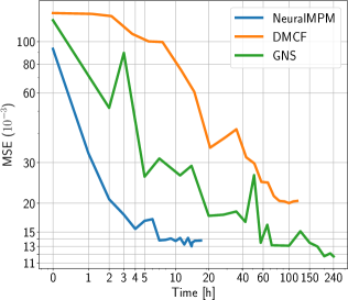
	$1$ Hour	$5$ Hours	$15$ Hours	Best	Ground Truth
Ours
GNS
DMCF

Figure 5: Training convergence. (Left) NeuralMPM trains and converges much faster than GNS and DMCF. Note the log scale on both axes. (Right) Snapshots of models trained for increasing durations then unrolled until the same timestep on a held-out simulation. For a fair comparison, out-of-bounds particles in GNS and DMCF were clamped.

	NeuralMPM (Ours)			GNS			DMCF
One model call ($T=1$)	8.04	$\pm$	0.43	13.91	$\pm$	2.83	12.85	$\pm$	8.41
Rollout ($T=600$)	606.63	$\pm$	7.69	8344.94	$\pm$	1700.8	9448.17	$\pm$	804.07

Table 2: Inference time (in ms) of NeuralMPM and baselines on WaterRamps. Times were averaged over all validation trajectories. NeuralMPM predicts 8 frames in a single model call and still outperforms the two baselines per call, which further widens the gap for the total rollout time. For comparison, [18] reports a computation time of 71ms to simulate one timestep with Taichi-MPM.

4.3 Generalization

One notable advantage of NeuralMPM is its invariance to the number of particles, as the transition model only processes the voxelized representation. To demonstrate this, we train a model on WaterRamps, which contains about $2.3$k particles and $600$ timesteps, and evaluate it on WaterDrop-XL, which features about four times more particles, $1000$ timesteps, and no obstacles. An example snapshot is displayed in Figure 6. Interestingly, the larger number of particles only affects interpolation steps between the grid and particles, resulting in a negligible impact on total inference time, making the model nearly as fast despite 4 times more particles. We also validate generalization quantitatively by comparing the error rates on WaterDrop-XL of a model trained directly on it and the model trained solely on WaterRamps. With the same training budget, the latter achieves a lower MSE at $20.92\times 10^{-3}$ against $28.09\times 10^{-3}$. More trajectories are displayed in Figure 10.

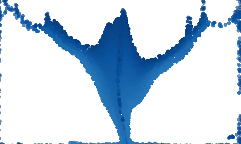
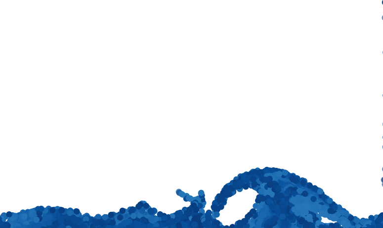
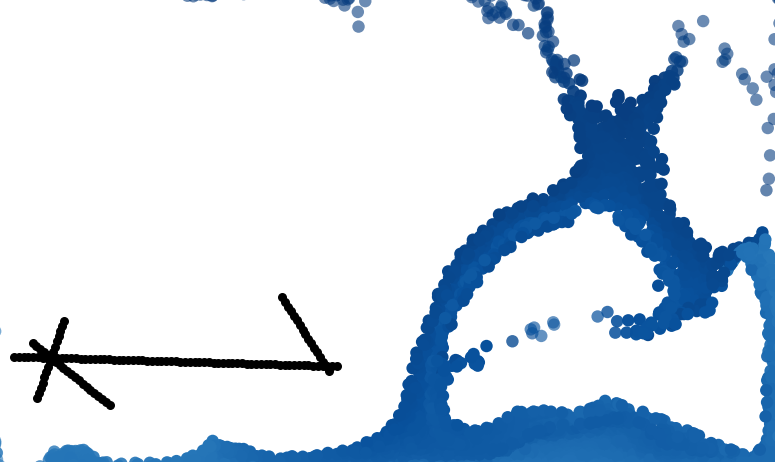
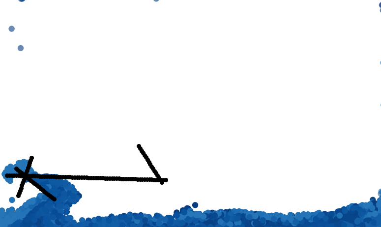
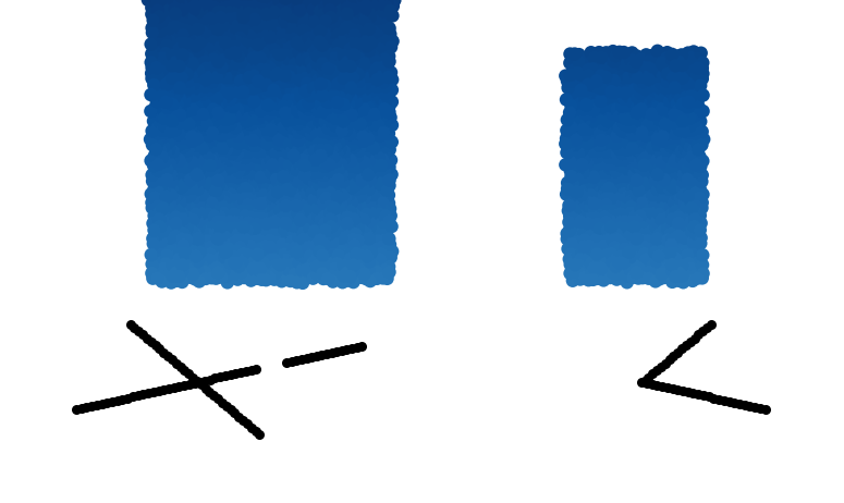
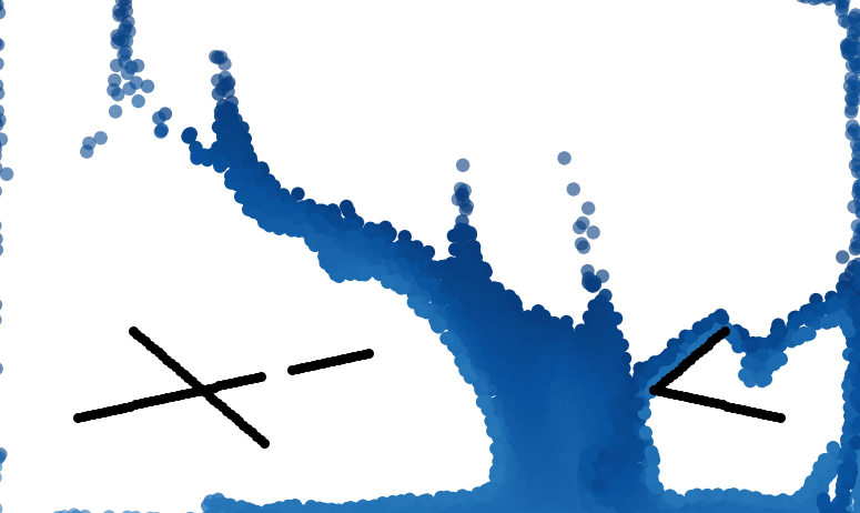
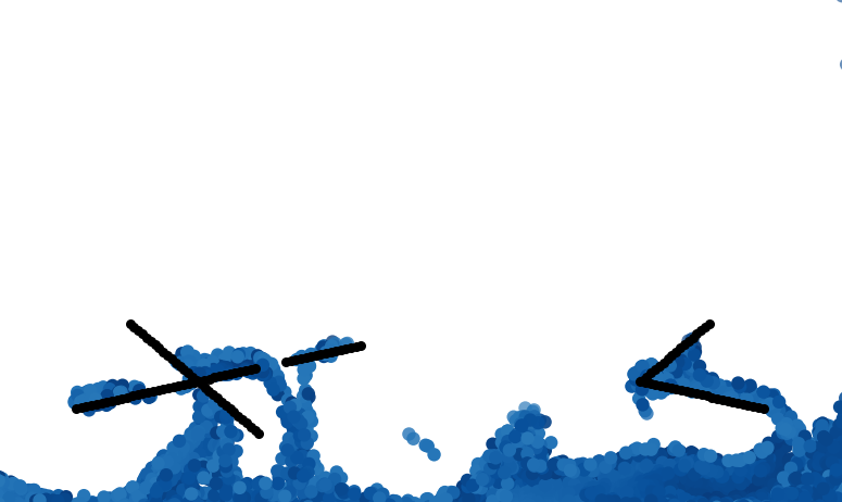
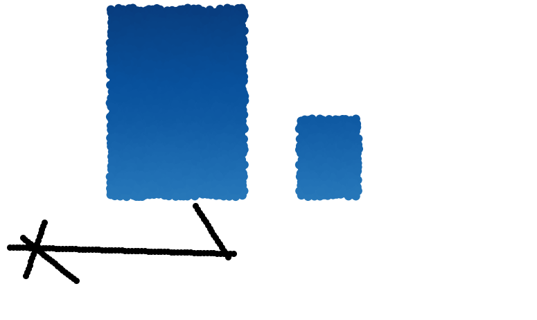
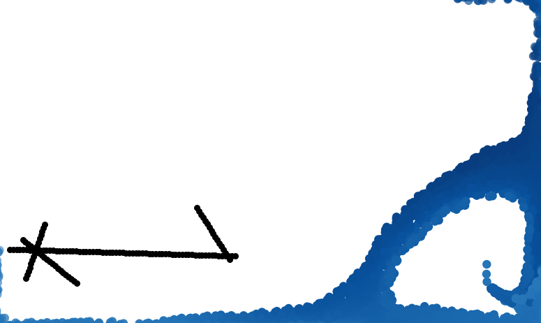
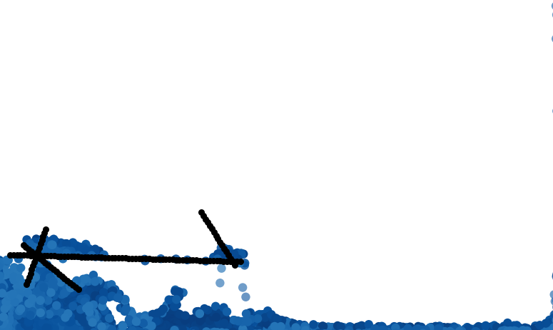
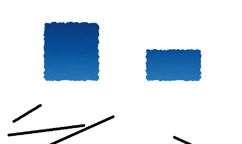
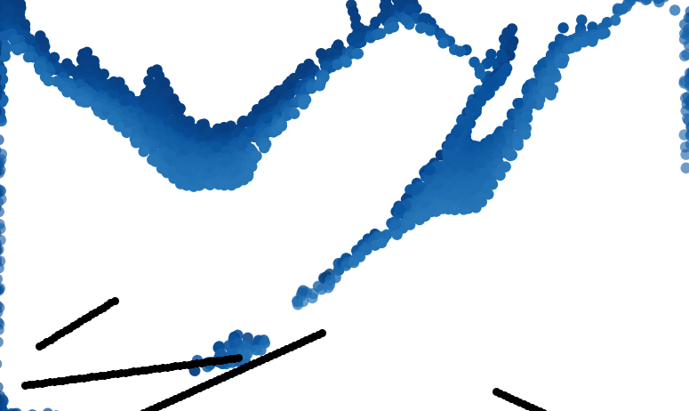
Figure 11: Generalization to larger and non-square domains. We train a model on the square domains in WaterRamps using $64\times 64$ input grids to the U-Net, and then perform inference on manually generated non-square environments that are twice as wide and use a $128\times 64$ input grid to the same U-Net. NeuralMPM flawlessly generalizes and emulates particles in these new environments. Note: no ground truth is available because the authors of GNS did not provide the physical parameters for simulating WaterRamps using Taichi. Chosen time steps are $0,150,575$. We recommend watching the videos in the supplementary material for more detailed evaluation.

If a domain-agnostic processor architecture is used, such as a fully convolutional U-Net or an FNO, then NeuralMPM can generalize to different domain shapes without retraining, as shown in Fig 6. We demonstrate this ability by considering a model solely trained on WaterRamps, a square domain of size $0.84\times 0.84$ mapped to $64\times 64$ grids. Without retraining, we perform inference with this model on larger unseen environments of size $1.68\times 0.84$, and change the grid size to $128\times 64$. The unseen environments were built by merging and modifying initial conditions of held-out test trajectories from WaterRamps. NeuralMPM manages to emulate particles in this larger and rectangular domain flawlessly despite being trained on a smaller domain with a smaller grid, showcasing the advantage of a U-Net for handling more general domains. No ground truth is displayed as [18] have not provided any information for simulating their data using Taichi-MPM. More trajectories are shown in Figure 11.

	WaterDrop-XL			Larger rectangular domains
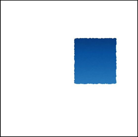
Initial						Initial
Predictions						Predictions $t_{1}$
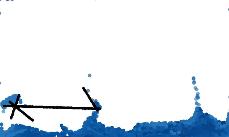
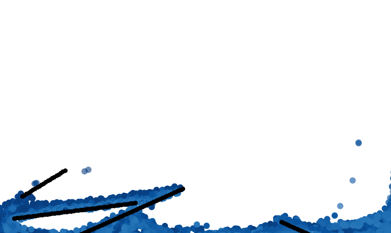
Ground Truth						Predictions $t_{2}$

Figure 6: Generalization. (Left) NeuralMPM generalizes to domains with more particles ($\sim 4\times$ here) with minimal inference time overhead due to the processing of the voxelized representation. (Right) A NeuralMPM model trained on a square domain can naturally generalize to larger rectangular domains (twice as wide here) when using a fully convolutional U-Net.

4.4 Inverse design problem

	Test 1	Test 2	Test 3
Initial
Unoptimized
Optimized

Figure 7: Inverse design problem. We exploit NeuralMPM’s differentiability to optimize the angle $\alpha$ of a ramp, anchored at the red dot, in order to get the water close to the red square region.

Finally, we demonstrate the application of NeuralMPM for inverse problems on a toy inverse design task that consists in optimizing the direction of a ramp to make the particles reach a target location, similar to [4]. We place a blob of water at different starting locations, and we then place a ramp at some location, with a random initial angle $\alpha$. The goal is to spin that ramp by tuning $\alpha$ in order to make the water end up at a desired location. The main challenges of this task are the long-range time horizon of the goal and the presence of nonlinear physical dynamics. We proceed by selecting the point where we want the water to end up and compute the average distance between the point and particles at the last simulation frame (Tests 1 & 2) or at an intermediate frame (Test 3). We then minimize the distance via gradient descent, leveraging the differentiability of NeuralMPM to solve this inverse design problem. We show three example optimizations in Figure 7.

5 Conclusion

Summary.

We presented NeuralMPM, a neural emulation framework for particle-based simulations inspired by the hybrid Eulerian-Lagrangian Material Point Method. We have shown its effectiveness in simulating a variety of materials and interactions, its ability to generalize to larger systems and its use in inverse problems. Crucially, NeuralMPM trains in a fraction of the time it takes to train alternative approaches, and is substantially faster at inference time. By interpolating particles onto a fixed-size grid, global information is distilled into a voxelized representation that is easier to learn and process with powerful image-to-image models. The use of voxelization allows NeuralMPM to bypass expensive graph constructions, and the interpolation leads to easier generalization to a larger number of particles and constant runtime. The lack of expensive graph construction and message passing also allows for more autoregressive steps and parallel rollouts.

Limitations.

Like other approaches, NeuralMPM is limited by the computation used to process the structure of the point cloud. In our case, voxelization means we cannot deal with particles that lie outside of the domain and are limited to regular grids. Additionally, the size of the voxels is directly related to the fluid’s density, defined as the number of particles within a given volume. If the voxels are too large, the model will fail to capture finer details. Conversely, if they are too small, the model may struggle due to insufficient local structure. Similarly, performance can degrade in very sparse domains. Compressible fluids might also present challenges, though this requires further verification.

Future work.

Our work is only a first step towards hybrid Eulerian-Lagrangian neural emulators, leaving many avenues for future research. Extending NeuralMPM to 3D systems is a natural continuation of this work. Future studies could also explore alternative particle-to-grid and grid-to-particle functions, like the non-uniform Fourier transform [57], or more sophisticated interpolation methods from classical MPM literature [22]. Additionally, incorporating features commonly used in classical SPH and MPM simulations, such as viscosity, pressure, or temperature, presents another promising direction for future work. A less traditional direction is to make NeuralMPM probabilistic and encode richer distributional information about the particles in the grid nodes, instead of maintaining only a mean value. This could potentially improve NeuralMPM’s ability to resolve subgrid phenomena. Advances in Lagrangian Particle Tracking [58] will eventually make it possible to create datasets from real-world data, enabling the training of NeuralMPM directly from data without the need for the costly design process of a numerical simulator. Lastly, losses that take into account the distribution of particles and are invariant under particle permutation, such as the earth mover’s distance, are increasingly becoming an option to consider, as more efficient differentiable approximations emerge.

Appendix A Training details

Hardware.

We run all our experiments using the same hardware: 4 CPUs, 24GB of RAM, and an NVIDIA RTX A5000 GPU with 24GB of VRAM. For reproducing the results of DMCF, we kept the A5000 GPU but it required up to 96GB of RAM for training.

Data Preprocessing.

Similar to [20], we slightly alter the original MPM datasets to add boundary particles, as the original data from [18] does not have them. We define the velocity at a timestep to be $\mathbf{v}_{t}=\mathbf{v}_{t}-\mathbf{v}_{t-1}$. We therefore skip the first step during training for which no velocity is available.

Implementation.

Our implementation, training scripts, experiment configurations, and instructions for reproducing results are publicly available at [URL]. We implement NeuralMPM using PyTorch [59], and use PyTorch Geometric [60] for implementing efficient particle-to-grid functions, more specifically from the Scatter and Cluster modules. For memory efficiency, we do not store all (up to) 1,000 training trajectories in memory, and rather use a buffer of about 16 trajectories over which several epochs are performed before loading a new buffer of random trajectories.

Baselines.

We use the official implementations and training instructions of GNS [18] and DMCF [20] to reproduce their results and conduct new experiments. More specifically, we train GNS as instructed for 5 million steps on all four datasets, using their provided configuration. For DMCF, we follow their default configurations, conducting 50k training iterations for WBC-SPH and 40k for WaterRamps, SandRamps, and Goop.

Normalization.

We normalize the input of the model over each channel individually. We investigated computing the statistics across a buffer, resembling [61], and precomputing them on the whole training set and found no difference in performance. During inference, we use the precomputed statistics.

Appendix B Supplementary results

Although we have used a U-Net architecture for the grid-to-grid processor, NeuralMPM can be used with any grid-to-grid processor and is not limited to that network. For example, in Figure 8 and Table 3 we present qualitative and quantitative ablation results, respectively, for NeuralMPM using an FNO network [51] as the grid-to-grid processor. Results show that the FNO processor is slightly worse than the U-Net processor.

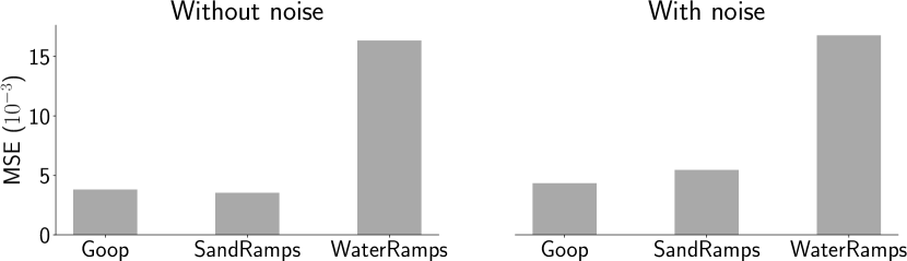
Figure 8: FNO processor. NeuralMPM with an FNO processor and default architecture. Rollout MSE ($\times 10^{-3}$) for different datasets.

Data	FNO with noise	FNO without noise
WaterRamps	16.8	16.3
SandRamps	5.5	3.5
Goop	4.3	3.8

Table 3: Rollout MSE ($\times 10^{-3}$) for NeuralMPM with an FNO processor and default architecture, with and without noise.

Table 4 reports the exact MSE rollout values that were reported in Figure 3 for Goop.

Parameter	Value	MSE ($\times 10^{-3}$)
$K$ (No noise)	$1$	3.2
	$2$	3.3
	$3$	2.4
	$4$	2.2
$K$ (With noise)	$1$	3.5
	$2$	2.5
	$3$	2.4
	$4$	3.0
Time bundling $m$	$1$	6.6
	$2$	4.5
	$4$	3.5
	$8$	2.1
	$16$	2.9
	$32$	3.5
Grid size	$32$	5.5
	$64$	2.4
	$128$	7.1

Parameter	Value	MSE ($\times 10^{-3}$)
Grid noise	$0$	3.2
	0.001	2.4
	0.005	6.9
Particle noise	$0$	2.2
	0.0003	2.4
	0.0006	2.4
	0.001	2.1
U-Net Depth	2	3.3
	3	3.0
	4	2.4
	5	2.3
U-Net Width	32	2.6
	64	2.3
	128	2.2

Table 4: Ablation results for Goop.

Finally, Figure 9 shows the error during rollouts for each dataset, both in terms of MSE and EMD. With both metrics, the error starts low and slowly accumulates over time. For the EMD, we use the Sinkhorn algorithm provided by [62].

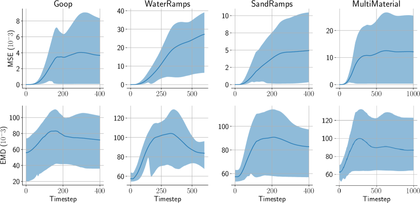
Figure 9: Error propagation during rollout. Shown is the mean and 80th percentile of the MSE and EMD, computed over particles and simulations, at each timestep during the rollout. The accuracy decreases as errors accumulate.

Appendix C Dam Break 2D (LagrangeBench)

In Table 5, we report the accuracy of NeuralMPM against the two baseline checkpoints provided in LagrangeBench [63]. Note that the values reported in Table 1 for GNS were reproduced by training for 20M steps following the indications of [18], which took about 12 days using the Jax implementation of LagrangeBench. NeuralMPM, on the other hand, took 7h. In Table 6, we report the inference times of NeuralMPM and the two baselines provided in LagrangeBench. Although these are more recent implementations of graph network-based simulators, NeuralMPM still outperforms them by a large margin.

	MSE$\downarrow$	EMD$\downarrow$
NeuralMPM (ours)	20.76	2.88
GNS [18]	114.40	224.1
SEGNN [56]	124.39	268.4

Table 5: Full-trajectory MSE ($\times 10^{-3}$) and Sinkhorn distance (EMD) ($\times 10^{-4}$) for NeuralMPM, GNS [18], and SEGNN [56] on the 2D Dam break dataset from LagrangeBench [63]. The two latter models are checkpoints provided by LagrangeBench. EMD is computed using the scripts provided by the authors.

	One model call ($T=1$)	Full rollout ($T=401$)	Average FPS
NeuralMPM (ours)	7.41	193.50	2072
GNS [18]	20.46	8,170.47	49
SEGNN [56]	46.04	18,194.10	22

Table 6: Inference time (in ms) of NeuralMPM, GNS [18], and [56] on the 2D Dam break dataset from LagrangeBench [63]. Times were averaged over all test trajectories. NeuralMPM predicts 16 frames in a single model call and still outperforms the two baselines per call, which further widens the gap for the total rollout time.

Appendix D Additional predicted trajectories

In addition to the trajectories in Figures 2 and 4, we show additional trajectories emulated with NeuralMPM for all datasets in Figures 12, 13, 14, 15, 17, and 16. We also release videos in the supplementary material, which we recommend watching to better see the details and limitations of NeuralMPM. This includes about 10 videos of emulated trajectories on held-out test simulations. Notably, we can observe the specific limitations of NeuralMPM on WBC-SPH, as shown in the latest trajectory depicted in Figure 16.

	$t=0$	$t=75$	$t=125$	$t=200$	$t=400$	$t=997$
Ground Truth
Prediction
Ground Truth
Prediction
Ground Truth
Prediction
Ground Truth
Prediction

Figure 10: Generalization to more particles on WaterDrop-XL. Snapshots of predicted trajectories emulated using a model trained solely on WaterRamps, against ground truth. All trajectories come from the held-out test set of WaterDrop-XL. To better show the differences of these longer sequences, we select the following timesteps not even in time: $t\in\{0,75,125,200,400,999\}$. We can observe that the generalizing model struggles to retain the shape of water while it’s falling.

	Initial Conditions	Snapshot 1	Snapshot 2

	$t=0$	$t=119$	$t=239$	$t=358$	$t=478$	$t=598$
Ground Truth
Prediction
Ground Truth
Prediction
Ground Truth
Prediction
Ground Truth
Prediction

Figure 12: Additional WaterRamps predicted trajectories. Evenly spaced in time snapshots of predicted unrolled trajectories against ground truth. All trajectories are from the held-out test set.

	$t=0$	$t=79$	$t=159$	$t=238$	$t=318$	$t=398$
Ground Truth
Prediction
Ground Truth
Prediction
Ground Truth
Prediction
Ground Truth
Prediction

Figure 13: Additional SandRamps predicted trajectories. Evenly spaced in time snapshots of predicted unrolled trajectories against ground truth. All trajectories are from the held-out test set.

	$t=0$	$t=32$	$t=65$	$t=97$	$t=130$	$t=398$
Ground Truth
Prediction
Ground Truth
Prediction
Ground Truth
Prediction
Ground Truth
Prediction

Figure 14: Additional Goop predicted trajectories. Snapshots of predicted unrolled trajectories against ground truth. All trajectories are from the held-out test set. Due to Goop quickly reaching equilibrium, more snapshots are taken in the first half of the trajectory.

	$t=0$	$t=119$	$t=239$	$t=358$	$t=478$	$t=598$
Ground Truth
Prediction
Ground Truth
Prediction
Ground Truth
Prediction
Ground Truth
Prediction

Figure 15: Additional MultiMaterial predicted trajectories. Evenly spaced in time snapshots of predicted unrolled trajectories against ground truth. All trajectories are from the held-out test set. The first trajectory illustrates a rare failure where the shape of sand particles is not retained, even though all particles are supposed to maintain the same velocity while airborne, as they are thrown against the wall.

	$t=0$	$t=100$	$t=300$	$t=500$	$t=700$	$t=3196$
Ground Truth
Prediction
Ground Truth
Prediction
Ground Truth
Prediction
Ground Truth
Prediction

Figure 16: Additional WBC-SPH predicted trajectories. Snapshots of predicted trajectories against ground truth. All trajectories come from the held-out test set. To better show the differences of these longer sequences, we select the following timesteps not even in time: $t\in\{0,100,300,500,700,3199\}$. In the last trajectory, NeuralMPM struggles to follow the gravity direction and breaks down over time.

	$t=0$	$t=125$	$t=400$
Ground Truth
Prediction
Ground Truth
Prediction
Ground Truth
Prediction
Ground Truth
Prediction

Figure 17: Additional Dam Break 2D predicted trajectories. Snapshots of predicted trajectories against ground truth. All trajectories come from the held-out test set. To better show the differences of these longer sequences, we select the following timesteps not even in time: $t\in\{0,125,400\}$. In the last trajectory, NeuralMPM struggles to follow the gravity direction and breaks down over time.

References

- Monaghan [2012] J.J. Monaghan. Smoothed particle hydrodynamics and its diverse applications. Annual Review of Fluid Mechanics, 44(Volume 44, 2012):323–346, 2012.
- Vacondio et al. [2021] Renato Vacondio, Corrado Altomare, Matthieu De Leffe, Xiangyu Hu, David Le Touzé, Steven Lind, Jean-Christophe Marongiu, Salvatore Marrone, Benedict D. Rogers, and Antonio Souto-Iglesias. Grand challenges for smoothed particle hydrodynamics numerical schemes. Computational Particle Mechanics, 8(3):575–588, 5 2021.
- Lind et al. [2020] Steven J. Lind, Benedict D. Rogers, and Peter K. Stansby. Review of smoothed particle hydrodynamics: towards converged lagrangian flow modelling. Proceedings of the Royal Society A: Mathematical, Physical and Engineering Sciences, 476(2241):20190801, 2020.
- Allen et al. [2022] Kelsey Allen, Tatiana Lopez-Guevara, Kimberly L Stachenfeld, Alvaro Sanchez Gonzalez, Peter Battaglia, Jessica B Hamrick, and Tobias Pfaff. Inverse design for fluid-structure interactions using graph network simulators. In S. Koyejo, S. Mohamed, A. Agarwal, D. Belgrave, K. Cho, and A. Oh, editors, Advances in Neural Information Processing Systems, volume 35, pages 13759–13774. Curran Associates, Inc., 2022.
- Zhao et al. [2022] Qingqing Zhao, David B Lindell, and Gordon Wetzstein. Learning to solve PDE-constrained inverse problems with graph networks. In Kamalika Chaudhuri, Stefanie Jegelka, Le Song, Csaba Szepesvari, Gang Niu, and Sivan Sabato, editors, Proceedings of the 39th International Conference on Machine Learning, volume 162 of Proceedings of Machine Learning Research, pages 26895–26910. PMLR, 7 2022.
- Liu et al. [2018] Zhaocheng Liu, Dayu Zhu, Sean P. Rodrigues, Kyu-Tae Lee, and Wenshan Cai. Generative model for the inverse design of metasurfaces. Nano Letters, 18(10):6570–6576, 10 2018.
- Colburn and Majumdar [2021] Shane Colburn and Arka Majumdar. Inverse design and flexible parameterization of meta-optics using algorithmic differentiation. Communications Physics, 4(1):65, 3 2021.
- Forte et al. [2022] Antonio Elia Forte, Paul Z. Hanakata, Lishuai Jin, Emilia Zari, Ahmad Zareei, Matheus C. Fernandes, Laura Sumner, Jonathan Alvarez, and Katia Bertoldi. Inverse design of inflatable soft membranes through machine learning. Advanced Functional Materials, 32(16):2111610, 2022.
- Kumar et al. [2020] Siddhant Kumar, Stephanie Tan, Li Zheng, and Dennis M. Kochmann. Inverse-designed spinodoid metamaterials. npj Computational Materials, 6(1):73, 6 2020.
- Lam et al. [2023] Remi Lam, Alvaro Sanchez-Gonzalez, Matthew Willson, Peter Wirnsberger, Meire Fortunato, Ferran Alet, Suman Ravuri, Timo Ewalds, Zach Eaton-Rosen, Weihua Hu, Alexander Merose, Stephan Hoyer, George Holland, Oriol Vinyals, Jacklynn Stott, Alexander Pritzel, Shakir Mohamed, and Peter Battaglia. Learning skillful medium-range global weather forecasting. Science, 382(6677):1416–1421, 2023.
- Pfaff et al. [2021] Tobias Pfaff, Meire Fortunato, Alvaro Sanchez-Gonzalez, and Peter Battaglia. Learning mesh-based simulation with graph networks. In International Conference on Learning Representations, 2021.
- Lemos et al. [2023] Pablo Lemos, Niall Jeffrey, Miles Cranmer, Shirley Ho, and Peter Battaglia. Rediscovering orbital mechanics with machine learning. Machine Learning: Science and Technology, 4(4):045002, 10 2023.
- Bourilkov [2019] Dimitri Bourilkov. Machine and deep learning applications in particle physics. International Journal of Modern Physics A, 34(35):1930019, December 2019.
- Jumper et al. [2021] John Jumper, Richard Evans, Alexander Pritzel, Tim Green, Michael Figurnov, Olaf Ronneberger, Kathryn Tunyasuvunakool, Russ Bates, Augustin Žídek, Anna Potapenko, Alex Bridgland, Clemens Meyer, Simon A. A. Kohl, Andrew J. Ballard, Andrew Cowie, Bernardino Romera-Paredes, Stanislav Nikolov, Rishub Jain, Jonas Adler, Trevor Back, Stig Petersen, David Reiman, Ellen Clancy, Michal Zielinski, Martin Steinegger, Michalina Pacholska, Tamas Berghammer, Sebastian Bodenstein, David Silver, Oriol Vinyals, Andrew W. Senior, Koray Kavukcuoglu, Pushmeet Kohli, and Demis Hassabis. Highly accurate protein structure prediction with alphafold. Nature, 596(7873):583–589, 8 2021.
- He et al. [2019] Siyu He, Yin Li, Yu Feng, Shirley Ho, Siamak Ravanbakhsh, Wei Chen, and Barnabás Póczos. Learning to predict the cosmological structure formation. Proceedings of the National Academy of Sciences, 116(28):13825–13832, June 2019.
- Nasser and Yusof [2023] Maged Nasser and Umi Kalsom Yusof. Deep learning based methods for breast cancer diagnosis: A systematic review and future direction. Diagnostics (Basel), 13(1), January 2023.
- Arpaia et al. [2021] P. Arpaia, G. Azzopardi, F. Blanc, G. Bregliozzi, X. Buffat, L. Coyle, E. Fol, F. Giordano, M. Giovannozzi, T. Pieloni, R. Prevete, S. Redaelli, B. Salvachua, B. Salvant, M. Schenk, M. Solfaroli Camillocci, R. Tomás, G. Valentino, F.F. Van der Veken, and J. Wenninger. Machine learning for beam dynamics studies at the cern large hadron collider. Nuclear Instruments and Methods in Physics Research Section A: Accelerators, Spectrometers, Detectors and Associated Equipment, 985:164652, January 2021.
- Sanchez-Gonzalez et al. [2020] Alvaro Sanchez-Gonzalez, Jonathan Godwin, Tobias Pfaff, Rex Ying, Jure Leskovec, and Peter Battaglia. Learning to simulate complex physics with graph networks. In Hal Daumé III and Aarti Singh, editors, Proceedings of the 37th International Conference on Machine Learning, volume 119 of Proceedings of Machine Learning Research, pages 8459–8468. PMLR, 7 2020.
- Ummenhofer et al. [2020] Benjamin Ummenhofer, Lukas Prantl, Nils Thuerey, and Vladlen Koltun. Lagrangian fluid simulation with continuous convolutions. In International Conference on Learning Representations, 2020.
- Prantl et al. [2022] Lukas Prantl, Benjamin Ummenhofer, Vladlen Koltun, and Nils Thuerey. Guaranteed conservation of momentum for learning particle-based fluid dynamics. In S. Koyejo, S. Mohamed, A. Agarwal, D. Belgrave, K. Cho, and A. Oh, editors, Advances in Neural Information Processing Systems, volume 35, pages 6901–6913. Curran Associates, Inc., 2022.
- Sulsky et al. [1993] Deborah Sulsky, Zhen Chen, and Howard L. Schreyer. A particle method for history-dependent materials. Computer Methods in Applied Mechanics and Engineering, 118:179–196, 1993.
- Nguyen et al. [2023] Vinh Phu Nguyen, Alban de Vaucorbeil, and Stéphane Bordas. The Material Point Method: Theory, Implementations and Applications (Scientific Computation) 1st ed. 2023 Edition. 02 2023. ISBN 3031240693.
- Nourian et al. [2016] Pirouz Nourian, Romulo Gonçalves, Sisi Zlatanova, Ken Arroyo Ohori, and Anh Vu Vo. Voxelization algorithms for geospatial applications: Computational methods for voxelating spatial datasets of 3d city models containing 3d surface, curve and point data models. MethodsX, 3:69–86, 2016.
- Xu et al. [2021] Yusheng Xu, Xiaohua Tong, and Uwe Stilla. Voxel-based representation of 3d point clouds: Methods, applications, and its potential use in the construction industry. Automation in Construction, 126:103675, 2021.
- Rakhsha et al. [2021] Milad Rakhsha, Christopher E. Kees, and Dan Negrut. Lagrangian vs. eulerian: An analysis of two solution methods for free-surface flows and fluid solid interaction problems. Fluids, 6(12), 2021.
- Iserles [2008] Arieh Iserles. A First Course in the Numerical Analysis of Differential Equations. Cambridge Texts in Applied Mathematics. Cambridge University Press, 2 edition, 2008.
- Morton and Mayers [2005] K. W. Morton and D. F. Mayers. Numerical Solution of Partial Differential Equations: An Introduction. Cambridge University Press, 2 edition, 2005.
- Wissing and Shen [2023] Robert Wissing and Sijing Shen. Numerical dependencies of the galactic dynamo in isolated galaxies with sph. Astronomy and Astrophysics, 673:A47, May 2023.
- Few et al. [2016] C. G. Few, C. Dobbs, A. Pettitt, and L. Konstandin. Testing hydrodynamics schemes in galaxy disc simulations. Monthly Notices of the Royal Astronomical Society, 460(4):4382–4396, 05 2016.
- Kegerreis et al. [2022] J. A. Kegerreis, S. Ruiz-Bonilla, V. R. Eke, R. J. Massey, T. D. Sandnes, and L. F. A. Teodoro. Immediate origin of the moon as a post-impact satellite. The Astrophysical Journal Letters, 937(2):L40, 2022.
- Gotoh and Khayyer [2016] Hitoshi Gotoh and Abbas Khayyer. Current achievements and future perspectives for projection-based particle methods with applications in ocean engineering. Journal of Ocean Engineering and Marine Energy, 2(3):251–278, 8 2016.
- Tan et al. [2023] Zhe Tan, Peng-Nan Sun, Nian-Nian Liu, Zhe Li, Hong-Guan Lyu, and Rong-Hua Zhu. Sph simulation and experimental validation of the dynamic response of floating offshore wind turbines in waves. Renewable Energy, 205:393–409, 2023.
- Lyu et al. [2022] Hong-Guan Lyu, Peng-Nan Sun, Xiao-Ting Huang, Shi-Yun Zhong, Yu-Xiang Peng, Tao Jiang, and Chun-Ning Ji. A review of sph techniques for hydrodynamic simulations of ocean energy devices. Energies, 15(2), 2022.
- Ionescu et al. [2005] Irina Ionescu, James Guilkey, Martin Berzins, Robert M Kirby, and Jeffrey Weiss. Computational simulation of penetrating trauma in biological soft tissues using the material point method. Stud Health Technol Inform, 111:213–218, 2005.
- Lu et al. [2006] Hongbing Lu, Nitin Daphalapurkar, B. Wang, Samit Roy, and Ranga Komanduri. Multiscale simulation from atomistic to continuum – coupling molecular dynamics (md) with the material point method (mpm). Philosophical Magazine, 86:2971–2994, 2006.
- Li and Liu [2002] Shaofan Li and Wing Kam Liu. Meshfree and particle methods and their applications. Applied Mechanics Reviews, 55(1):1–34, 01 2002.
- York II et al. [2000] Allen R. York II, Deborah Sulsky, and Howard L. Schreyer. Fluid–membrane interaction based on the material point method. International Journal for Numerical Methods in Engineering, 48(6):901–924, 2000.
- Daphalapurkar et al. [2007] Nitin P. Daphalapurkar, Hongbing Lu, Demir Coker, and Ranga Komanduri. Simulation of dynamic crack growth using the generalized interpolation material point (gimp) method. International Journal of Fracture, 143(1):79–102, 01 2007.
- Llano Serna et al. [2015] Marcelo Alejandro Llano Serna, Márcio Muniz-de Farias, and Hernán Eduardo Martínez-Carvajal. Numerical modelling of alto verde landslide using the material point method. DYNA, 82(194):150–159, 11 2015.
- Stomakhin et al. [2013] Alexey Stomakhin, Craig Schroeder, Lawrence Chai, Joseph Teran, and Andrew Selle. A material point method for snow simulation. ACM Trans. Graph., 32(4), 07 2013.
- Brandstetter et al. [2022a] Johannes Brandstetter, Daniel E. Worrall, and Max Welling. Message passing neural PDE solvers. In International Conference on Learning Representations, 2022a.
- List et al. [2024] Bjoern List, Li-Wei Chen, Kartik Bali, and Nils Thuerey. How temporal unrolling supports neural physics simulators, 2024. URL https://arxiv.org/abs/2402.12971.
- Sharabi and Louppe [2023] Omer Rochman Sharabi and Gilles Louppe. Trick or treat? evaluating stability strategies in graph network-based simulators. 2023. URL https://api.semanticscholar.org/CorpusID:268033249.
- Han et al. [2022] Jiaqi Han, Wenbing Huang, Hengbo Ma, Jiachen Li, Josh Tenenbaum, and Chuang Gan. Learning physical dynamics with subequivariant graph neural networks. Advances in Neural Information Processing Systems, 35:26256–26268, 2022.
- Zhang et al. [2020] Yalan Zhang, Xiaojuan Ban, Feilong Du, and Wu Di. Fluidsnet: End-to-end learning for lagrangian fluid simulation. Expert Systems with Applications, 152:113410, 2020. ISSN 0957-4174. doi: https://doi.org/10.1016/j.eswa.2020.113410. URL https://www.sciencedirect.com/science/article/pii/S0957417420302347.
- Hastings and Mesit [2005] Erin Hastings and Jaruwan Mesit. Optimization of large-scale, real-time simulations by spatial hashing. January 2005.
- Yin et al. [2021] Yuan Yin, Vincent Le Guen, Jérémie Dona, Emmanuel de Bézenac, Ibrahim Ayed, Nicolas Thome, and Patrick Gallinari. Augmenting physical models with deep networks for complex dynamics forecasting*. Journal of Statistical Mechanics: Theory and Experiment, 2021(12):124012, December 2021. ISSN 1742-5468. doi: 10.1088/1742-5468/ac3ae5. URL http://dx.doi.org/10.1088/1742-5468/ac3ae5.
- Li et al. [2024] Jin Li, Yang Gao, Ju Dai, Shuai Li, Aimin Hao, and Hong Qin. Mpmnet: A data-driven mpm framework for dynamic fluid-solid interaction. IEEE Transactions on Visualization and Computer Graphics, 30(8):4694–4708, August 2024. ISSN 2160-9306. doi: 10.1109/tvcg.2023.3272156. URL http://dx.doi.org/10.1109/TVCG.2023.3272156.
- Ma et al. [2023] Pingchuan Ma, Peter Yichen Chen, Bolei Deng, Joshua B. Tenenbaum, Tao Du, Chuang Gan, and Wojciech Matusik. Learning neural constitutive laws from motion observations for generalizable pde dynamics, 2023. URL https://arxiv.org/abs/2304.14369.
- Ronneberger et al. [2015] Olaf Ronneberger, Philipp Fischer, and Thomas Brox. U-net: Convolutional networks for biomedical image segmentation. In Medical image computing and computer-assisted intervention–MICCAI 2015: 18th international conference, Munich, Germany, October 5-9, 2015, proceedings, part III 18, pages 234–241. Springer, 2015.
- Li et al. [2021] Zongyi Li, Nikola Borislavov Kovachki, Kamyar Azizzadenesheli, Burigede liu, Kaushik Bhattacharya, Andrew Stuart, and Anima Anandkumar. Fourier neural operator for parametric partial differential equations. In International Conference on Learning Representations, 2021.
- Hu et al. [2018] Yuanming Hu, Yu Fang, Ziheng Ge, Ziyin Qu, Yixin Zhu, Andre Pradhana, and Chenfanfu Jiang. A moving least squares material point method with displacement discontinuity and two-way rigid body coupling. ACM Trans. Graph., 37(4), 07 2018.
- Adami et al. [2012] S. Adami, X.Y. Hu, and N.A. Adams. A generalized wall boundary condition for smoothed particle hydrodynamics. Journal of Computational Physics, 231(21):7057–7075, 2012.
- Kingma and Ba [2014] Diederik P Kingma and Jimmy Ba. Adam: A method for stochastic optimization. arXiv preprint arXiv:1412.6980, 2014.
- Loshchilov and Hutter [2017] Ilya Loshchilov and Frank Hutter. SGDR: Stochastic gradient descent with warm restarts. In International Conference on Learning Representations, 2017.
- Brandstetter et al. [2022b] Johannes Brandstetter, Rob Hesselink, Elise van der Pol, Erik J Bekkers, and Max Welling. Geometric and physical quantities improve e(3) equivariant message passing. In International Conference on Learning Representations, 2022b.
- Fessler and Sutton [2003] J.A. Fessler and B.P. Sutton. Nonuniform fast fourier transforms using min-max interpolation. IEEE Transactions on Signal Processing, 51(2):560–574, 2003.
- Schröder and Schanz [2023] Andreas Schröder and Daniel Schanz. 3d lagrangian particle tracking in fluid mechanics. Annual Review of Fluid Mechanics, 55(Volume 55, 2023):511–540, 2023. ISSN 1545-4479.
- Paszke et al. [2019] Adam Paszke, Sam Gross, Francisco Massa, Adam Lerer, James Bradbury, Gregory Chanan, Trevor Killeen, Zeming Lin, Natalia Gimelshein, Luca Antiga, et al. Pytorch: An imperative style, high-performance deep learning library. Advances in neural information processing systems, 32, 2019.
- Fey and Lenssen [2019] Matthias Fey and Jan Eric Lenssen. Fast graph representation learning with pytorch geometric. arXiv preprint arXiv:1903.02428, 2019.
- Ioffe and Szegedy [2015] Sergey Ioffe and Christian Szegedy. Batch normalization: Accelerating deep network training by reducing internal covariate shift. In International conference on machine learning, pages 448–456. pmlr, 2015.
- Cuturi et al. [2022] Marco Cuturi, Laetitia Meng-Papaxanthos, Yingtao Tian, Charlotte Bunne, Geoff Davis, and Olivier Teboul. Optimal transport tools (ott): A jax toolbox for all things wasserstein. arXiv preprint arXiv:2201.12324, 2022.
- Toshev et al. [2024] Artur Toshev, Gianluca Galletti, Fabian Fritz, Stefan Adami, and Nikolaus Adams. Lagrangebench: A lagrangian fluid mechanics benchmarking suite. Advances in Neural Information Processing Systems, 36, 2024.