Spectrum correction on Ekman-Navier-Stokes equation in two-dimensions

Abstract

It has been long known that the addition of linear friction on two-dimensional Navier-Stokes (NS) turbulence, often referred to as Ekman-Navier-Stokes (ENS) turbulence, induces strong intermittent fluctuations on small-scale vorticity. Such fluctuations are strong enough to be measurable at low-order statistics such as the energy or enstrophy spectrum. Simple heuristics lead to corrections in the spectrum which are proportional to the linear friction coefficient. In this work, we study the spectral correction by the implementation of a GPU-accelerated high-resolution numerical simulation of ENS covering a large range of Reynolds numbers. Among our findings, we highlight the importance of non-locality when comparing the expected results to the measured ones.

I Introduction

Turbulence is a complex and fascinating phenomenon that happens in nature at different physics scales ranging from upper ocean dynamics [1], passing through planetary atmosphere [2], to interstellar media [3] and so on. The beauty of this phenomenon is not restricted to its observation in nature, but also to the fact that a single set of dynamic equations is responsible for all those complexities, the Navier-Stokes (NS) equations [4]. The non-linear and non-local nature of the NS equations requires numerical techniques to solve it within a numerical precision, to advance the understanding of turbulence phenomena.

The need for larger and larger simulations has been growing over time at the same rate as the hardware capabilities since numerical simulations are required to solve large and small scales at once [celani2007frontiers]. Efficient numerical techniques such as the pseudospectral method [5, 6] and the use of massive CPU (Computing Processor Unit) parallelization [7, 8] became the usual paradigm on computational turbulence in the idealized case of homogeneous-isotropic conditions. This combination relies on the fact that multidimensional Fast Fourier Transform (FFT), the basic core of the pseudospectral method, can be decomposed as a sequence of lower dimensional FFTs [9]. The latter method slices the spatial domain into many small packs of data and, through all-to-all CPU communications accelerates the computation of the most intensive parts of the NS solvers by performing concurrently low dimensional FFTs.

GPU (Graphical Processor Unit) started to be used as auxiliary devices (usually called accelerators) to enhance computational gain on each spatially decomposed piece of data as the GPUs have many more cores than single CPUs [10, 11]. GPU accelerators pushed the computation runtime to a point where almost all the computation time is spent on data transferring and communication among different devices [12, 13]. Fortunately, GPU manufacturers such as NVIDIA and AMD have been developing new devices with larger memories and/or faster inter-GPU connections, leading to huge accelerations in communications. New GPU technologies and their applications on the main supercomputing centers enabled extensive turbulence simulations up to $32768^{3}$ spatial gridpoints on feasible computational timescales [14].

Notwithstanding, several physical settings in the $\alpha$-turbulence model [15], thin layer turbulence [16, 17, 18, 19, 20], rotating and/or stratified turbulence [21, 22, 23], and many others, have almost identical dynamical equations and, in some cases, do not require extremely high spatial resolution to be studied. However, since those systems can display poor statistical convergence, they need to be solved for very long times or need to cover a parameter space of large dimensions.

The most popular way of writing numerical code on GPU is by using CUDA, a parallel computing platform created by NVIDIA that provides drop-in accelerated libraries such as FFT and linear algebra libraries. One of its strong points is its availability of the most familiar computational languages such as C/C^#/C⁺⁺, Fortran, Java, Python, etc. However, the CUDA solution has a closed code and works only for NVIDIA-based hardware, losing its interoperability among different hardware platforms and clusters. On the other hand, the Hybrid Input-Output (HIT) is an open-source low-level language with a syntax that is similar to CUDA. Employing HIT or similar open-source languages such as OpenCL, developers can ensure the portability and maintainability of their code among heterogeneous platforms. In summary, even though GPU coding options and interfaces have evolved, it is still needed for inexperienced developers to completely dive into one or more languages to be able to develop heterogeneous applications on GPU.

From the point of view of applications, the use of GPU to accelerate partial differential equations computations does not usually require to write completely new code, but simply to port an existing one [24, 25]. If one is restricted to NVIDIA platforms, a possible solution, is less efficient but much easier, is OpenACC, a directive-based programming model that simplifies parallel GPU programming. Using compiler directives for C and Fortran, OpenACC allows developers to port their existing CPU code, specifying which parts should be offloaded to the GPU for acceleration, and also supporting Message Passing Interface (MPI) for multi-node, multi-GPU applications.

The focus of this work is to present a single GPU solution for a generalized Navier-Stokes equation in two dimensions. Sec. II revisits the phenomenology of 2D turbulence in the presence of linear large-scale friction, usually referred to as Ekman friction. In Sec. III we introduce the standard pseudospectral method for solving the generalized equation showing some performance tests. Sec. IV applies our numerical solver to revisit the problem of spectrum correction, focusing on the specific case of the correction to the scaling exponent of the energy spectrum due to the linear friction, concluding with Sec. V where we discuss the results pointing directions of future research.

II Direct cascade in two-dimensional Navier-Stokes equation

It has long been known that studying the 2D NS equation is more than simply an academic case study on the road to understanding turbulence phenomena. The Earth’s atmosphere [26], the dynamics of oceans’ surface [27], and geometrically confined flows [17, 19] are examples of physical systems where experiments and numerical simulations show feature of two-dimensional turbulence, at least on a range of scales. To revisit the 2D phenomenology, we start with the incompressible Navier-Stokes equation in two dimensions

$$\begin{cases}\partial_{t}v_{i}+v_{j}\nabla_{j}v_{i}+\nabla_{i}P=\nu\nabla^{2}v_{i}-\mu v_{i}+F_{i}\ ,&\\ \nabla_{i}v_{i}=0\ ,\ \end{cases}$$ (1)

where repeated indices are implicitly summed and $\nabla_{i}\equiv\partial/\partial x_{i}$ are the components of the gradient vector. The field $v_{i}(\vec{x},t)$ represents the fluid velocity, $P(\vec{x},t)$ is the pressure field whose role is to ensure incompressibility and $F_{i}(\vec{x},t)$ represents an external forcing density. Two dissipative terms are in (1), one is the standard viscosity $\nu\nabla^{2}v_{i}$ which is active at small scales, while $\mu v_{i}$, often referred to as Ekman friction, remove energy at large scales and provide a statistically stationary state. This friction term has a different physical origin depending on the specific physical model, e.g. layer-layer friction in stratified fluids [28] or air friction in the case of soap films [31].

2D incompressible NS equations can be conveniently rewritten in terms of a pseudoscalar vorticity and the stream function. The former is given by $\omega=\epsilon_{ij}\nabla_{i}v_{j}$ while the latter is related to the velocity field through $v_{i}=\epsilon_{ij}\nabla_{j}\psi$ where in both cases, $\epsilon_{ij}$ is the full antisymmetric tensor. Clearly, we have $\omega=-\nabla^{2}\psi$. By contracting (1) with $\epsilon_{ji}\nabla_{j}$ we get

$$\partial_{t}\omega+J(\omega,\psi)=\nu\nabla^{2}\omega-\mu\omega+f\ ,\$$ (2)

where the Jacobian is $J(\omega,\psi)=\epsilon_{ij}\nabla_{i}\omega\nabla_{j}\psi=\nabla_{i}\left(v_{i}\omega\right)$ and $f=\epsilon_{ij}\nabla_{i}F_{j}$ is the 2D curl of the forcing.

A convenient assumption for the study of homogeneous-isotropic turbulence is to assume that the forcing $f(x,t)$ is a random function with zero mean and white-in-time correlations:

$$\left\langle f(\vec{x},t)f(\vec{y},s)\right\rangle=\delta(t-s)\xi(|\vec{x}-\vec{y}|)\ ,\$$ (3)

where the spatial correlation function has support on a given scale, i.e. $\xi(|\vec{x}|\approx\ell_{f})\approx\xi_{0}$, and $\xi(|\vec{x}|\gg\ell_{f})\rightarrow 0$.

In the inviscid, unforced limit, the model (2) conserved the kinetic energy $E=\left\langle|{\bm{v}}|^{2}\right\rangle/2$ and the enstrophy $Z=\left\langle\omega^{2}\right\rangle/2$, where the brackets indicate the average over the domain. In the presence of forcing and dissipations the energy/enstrophy balances read

$$\frac{dE}{dt}=-2\nu Z-2\mu E+\left\langle{\bf v}\cdot{\bf F}\right\rangle=-\varepsilon_{\nu}-\varepsilon_{\mu}+\varepsilon_{I}$$ (4)

and

$$\frac{dZ}{dt}=-2\nu P-2\mu Z+\left\langle\omega f\right\rangle=-\eta_{\nu}-\eta_{\mu}+\eta_{I}$$ (5)

The different terms in (4-5) define the characteristic scales of forcing $\ell_{f}=2\pi\sqrt{\varepsilon_{I}/\eta_{I}}$, viscous dissipation $\ell_{\nu}=2\pi\sqrt{\varepsilon_{\nu}/\eta_{\nu}}$ and friction $\ell_{\mu}=2\pi\sqrt{\varepsilon_{\mu}/\eta_{\mu}}$. When these scales are well separated $\ell_{\nu}\ll\ell_{f}\ll\ell_{\mu}$ and in stationary conditions one expects the development of a direct enstrophy cascade in the inertial range of scales $\ell_{\nu}\leq\ell\leq\ell_{f}$ and an inverse energy cascade in the scales $\ell_{f}\leq\ell\leq\ell_{\mu}$ [35] (see Appendix A).

The central statistical object in the classical theory of turbulence is the energy spectrum $E(k)$ defined as $\int E(k)dk=E$. In the range of scales $\ell_{\nu}\leq\ell\leq\ell_{f}$ dissipative effects are negligible and can assume a constant flux of enstrophy $\Pi_{Z}(k)$. This can be expressed in terms of the energy spectrum as [35]

$$\Pi_{Z}(k)=\lambda_{k}E(k)k^{3}$$ (6)

where $\lambda_{k}$ is the characteristic frequency of deformation of eddies at the scale $1/k$. Dimensionally one has

$$\lambda_{k}^{2}=\int_{k_{f}}^{k}E(p)p^{2}dp$$ (7)

where $k_{f}=2\pi/\ell_{f}$ is the wavenumber associated to the forcing and the upper limit in the integral reflects that scales smaller than $1/k$ act incoherently. A scale-free solution that gives a constant enstrophy flux $\Pi_{Z}(k)=\eta$ gives $E(k)\simeq\eta^{2/3}k^{-3}$. However, this is not consistent since this gives, when inserted in (7) and (6), a log-dependent enstrophy flux. In other words, a scale-independent flux is not compatible with a pure power-law energy spectrum. The correction proposed by Kraichnan is to include a log-correction in the spectrum [36]

$$E(k)\simeq\eta_{\nu}^{2/3}k^{-3}\left[\ln(k/k_{f})\right]^{-1/3}$$ (8)

which now gives a scale-independent enstrophy flux.

One important remark for the following is that the spectrum (8) gives a log-dependency of the frequencies $\lambda_{k}$ on the wavenumber. Therefore the direct cascade of enstrophy is at the border of locality in the sense that all the scales contribute with the same rate to the transfer of enstrophy.

While viscous dissipation simply acts as a high-wavenumber cut-off of the constant enstrophy flux and the Kraichnan spectrum (8), the role of friction is more subtle as it produces a correction to the exponent of the spectrum and even the breakdown of self-similar scaling [40, bernard2000influence]. This effect is strictly related to the non-local property of the cascade. Indeed in the presence of friction one can write a simple expression for the rate of enstrophy transfer [35]

$$\frac{d\Pi_{Z}(k)}{dk}=-\mu k^{2}E(k)$$ (9)

which states that part of the flux is removed in the cascade at a rate proportional to the friction coefficient $\mu$. Using now (6) with a constant deformation rate $\lambda_{k}=\lambda_{k_{f}}$ one immediately obtain the solution

$$E(k)\sim k^{-(3+\xi)}$$ (10)

with the correction in the power-law scaling

$$\xi=\frac{\mu}{\lambda_{k_{f}}}\,.$$ (11)

A posteriori, the use of a constant deformation rate $\lambda_{k_{f}}$ is justified by the fact that inserting (10) (with any $\xi>0$) into (7) produces a deformation frequency which decreases with $k$ and therefore $k_{f}$ is the most efficient scale in the transfer of enstrophy.

We remark that the above argument can be made more rigorous in the physical space where $\lambda_{k_{f}}$ is replaced by the Lyapunov exponent of the smooth flow. By taking into account its finite-time fluctuations one predicts the breakdown of self-similar scaling and the production of intermittency in the statistics of the vorticity field [40] which has been observed in numerical simulations [37].

III Numerical simulations of the direct cascade with friction

We tested the prediction of the previous Section, and in particular the correction (10) to the energy spectrum in the presence of friction, by means of extensive direct numerical simulations of the 2D NS equations (2) at very high resolutions using a pseudo-spectral code implemented on Nvidia GPU using the directive-based programming model OpenACC. Some details about the code and its performances can be found in Appendix A.

Simulations are done in a square box of size $L_{x}=L_{y}=2\pi$, with regular grid $N=N_{x}=N_{y}$ with forcing correlation given by (3). Three sets of simulations have been done with different resolution and viscosity $\nu$, with different values of the friction coefficient $\mu$ in each set.

Run	$N$	$\nu$	$k_{f}\pm\Delta k$	$\eta_{I}$	$Re_{\nu}$	$k_{\max}\ell_{\nu}$	$\mu\times 10^{2}$
A	4096	$2\times 10^{-5}$	$8\pm 1$	9.615	65584	4.19	1,4,7,10,20,30,40,50,60,80
B	8192	$5\times 10^{-6}$	$16\pm 1$	34.560	100463	3.38	4,6,10,20,30,40,50,60,80,100
C	16384	$1.25\times 10^{-6}$	$32\pm 1$	114.750	149877	2.77	6,12,18,36,48,60,72,96,120

Table 1: Most relevant parameters of the simulation including, $\ell_{f}=2\pi/k_{f}$, and $k_{\max}=N/3$ since we use the 2/3 de-aliasing method. The viscous scale and the Reynolds number are given by $\ell_{\nu}=\nu^{1/2}\eta_{I}^{-1/6}$ and $Re_{\nu}=\left(\ell_{\nu}/\ell_{f}\right)^{2}$. Both numbers should be taken as lower bound estimation since, if one considers $\eta_{\nu}$ instead of $\eta_{I}$ as a proper flux scale, one has bigger numbers since $\eta_{\nu}\leq\eta_{I}$.

We changed the forcing scale to allow, for the simulations at the highest resolution, the development of a narrow inverse cascade to study its effect on the phenomenology of the direct cascade. Table 1 shows the most relevant parameters of our simulations.

Fig. 1 shows some snapshots of the vorticity field taken from numerical simulations at different resolutions. The size of the largest vortices observed in the flow corresponds to the forcing scale which is reduced increasing the resolution, as indicated in Table 1. By zooming the runs by the factor corresponding to the different forcing scales, we see indeed that the vortices are rescaled approximatively to the same scale.

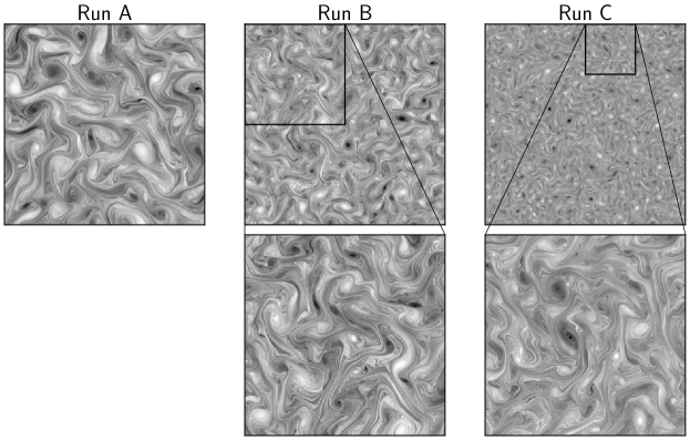
Figure 1: Snapshot of $\omega(x,y)$ for different Runs A, B, and C, with $\mu=4\times 10^{-2}$, $4\times 10^{-2}$, and $6\times 10^{-2}$, respectively. Zoomed regions span an area of $(4\ell_{f})^{2}$.

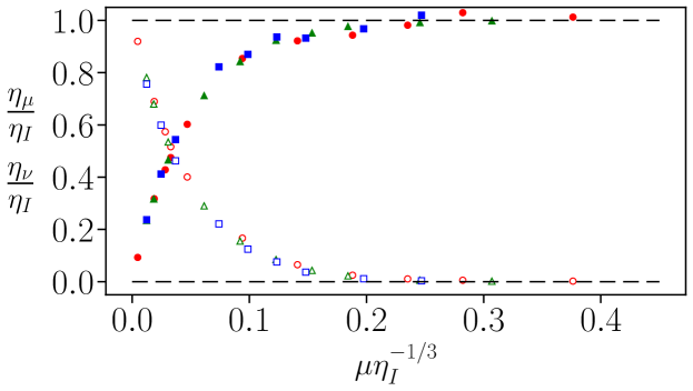
Figure 2: Ratio of viscous enstrophy dissipation $\eta_{\nu}$ (open symbols) and of the friction dissipation $\eta_{\mu}$ (full symbols) to the enstrophy input $\eta_{I}$ for the runs A, B, and C as circles, triangles, and squares, respectively. The x-axis is made nondimensional using $\eta_{I}$ since it is prescribed on all simulations.

The enstrophy balance (5) is shown in Fig. 2 for all the simulations in stationary conditions. Remarkably, this quantity is independent on the resolution (i.e. on the viscosity) and depends on the dimensionless parameter $\mu\eta_{I}^{1/3}$ only. We see that for $\mu\eta_{I}^{1/3}\gtrsim 0.2$ all the enstrophy in the cascade is removed by friction term.

Figure 3 shows the time-averaged energy spectra for the different simulations of the set C at the highest resolution. In all cases, in the direct cascade range, the spectrum displays a power-law scaling steeper than $k^{-3}$ and the steepness increases for larger values of the friction coefficient. The runs with the smallest values of friction display a short inverse cascade at wavenumber $k<k_{f}$ with an exponent close to the dimensional prediction $k^{-5/3}$.

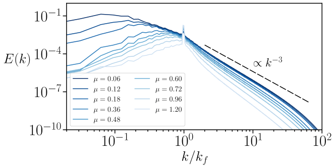
Figure 3: Stationary energy spectra from the simulations of set C for different friction parameters $\mu$.

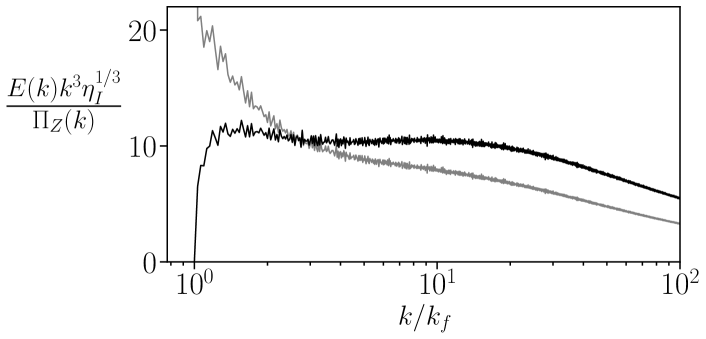
Figure 4: Compensated spectrum over flux as functions of the wavenumber. The darker curve is compensated also with the log-correction term.

In order to measure the correction $\xi(\mu)$ to the scaling exponent we fitted $E(k)k^{3}$ with a pure power-law behavior. We found that this procedure is not very robust since it depends on the range of wavenumbers chosen for the fit. Indeed, a non-power-law behavior is observed for wavenumber $k\gtrsim k_{f}$, as it is evident from Fig. 3. Moreover, we find that even for finite $\mu$ the relation (6) between the spectrum and the enstrophy flux requires the introduction of a logarithmic correction. This is evident from Fig. 4 where we plot the ratio $E(k)k^{3}\ln(k/k_{f})^{1/3}/\Pi_{Z}(k)$ together with $E(k)k^{3}/\Pi_{Z}(k)$ for run C. It is evident that while the latter quantity is never constant, the incorporation of the logarithmic term produces a constant ratio on the inertial range of scales.

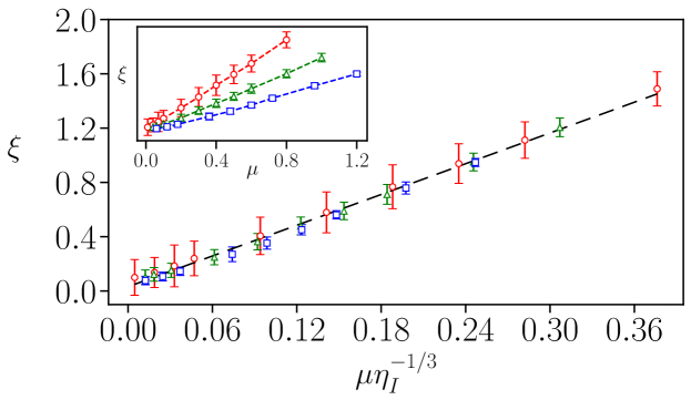
Figure 5: Scaling exponent correction $\xi$ as a function of the dimensionless friction coefficient $\mu/\eta_{I}^{1/3}$ for the simulations of the set A (red circles), B (green triangles) and C (blue squares). The dashed line represents the fit $\xi=4\mu/\eta_{I}^{1/3}$. Inset: the exponent correction $\xi$ as a function of $\mu$ for the three sets of simulations.

We therefore measure the exponent correction $\xi(\mu)$ by a power-law fit of the compensated energy spectra $E(k)k^{3}\ln(k/k_{f})^{1/3}$. The results are shown in Fig. 5 for all our simulations. We find that the correction is indeed linear with the friction coefficient $mu$, as predicted by (11) with a different slope for the different sets of simulations. The deformation rate $\lambda_{k_{f}}$ in (11) is dimensionally an inverse time and this suggests to plot the exponents of the different runs as a function of the dimensionless friction $\mu/\eta_{I}^{1/3}$. In Fig. 5 we see that indeed this produces an almost perfect collapse of the data from the different runs. We remark that the above rescaling is not a unique possibility: Indeed an inverse time of the flow is also given by $\eta_{\nu}^{1/3}$ or $Z^{1/2}$ but we find that data collapse is observed with the proposed compensation only.

IV Conclusions

In this paper, we offer a GPU-accelerated solution for high-resolution numerical simulations of generalized convection-diffusion equations in two dimensions. The use of a single GPU permits huge accelerations due to the absence of inter-GPU communication. This paradigm shift permitted an acceleration of about $40$ times respectively to the CPU code. Since GPU memories are the huge bottleneck of the application, the best use for our code are problems that do not require too big spatial resolution but still need to solve many large time scales. One among many examples is the study of non-equilibrium fluctuation on SQG turbulence [47]. Indeed, the latter work used a preliminary version of the present code.

For our physical application, we studied the 2D NS equations in the presence of Ekman friction, revisiting low-resolution results on its energy spectra that exhibit a steeper power-law decay than predicted by dimensional analysis, consistent with the presence of intermittency. This steepness increases linearly with friction, aligning with the theoretical prediction $E(k)\sim k^{-(3+\xi)}$, where $\xi=2\mu/\bar{\lambda}$ put forward by [37]. Furthermore, in our simulations, we permitted the existence of an inverse energy cascade that, in principle, should invalidate the arguments leading to the linear dependency of the correction on the friction parameter. For the latter, we notice that as long the turbulent state is not of a condensate, the linear prediction holds.

Regarding the infinite time Lyapunov exponent $\bar{\lambda}$, our results show that it is the inverse of twice the large scale time $\tau_{f}=\eta_{I}^{-1/3}$, instead of the small scale quantities. Future investigations could delve deeper into the specific mechanisms through which large-scale dynamics influence $\bar{\lambda}$ by the proper estimation of the Cramer function, potentially shedding light on fundamental aspects of turbulence intermittency and the passiveness of vorticity at small scales. In this sense, adding the implementation of passive scalar, eulerian/lagrangian tracers, and possible multiple GPU implementations on the gTurbo code is likely to be developed in the near future.

*

Appendix A Numerical integration of the 2D NS equation

To build numerical solvers for a broader class of turbulent models, we rewrite (2) in a more general formulation,

$$(\partial_{t}+\mathcal{L}_{\nu,\mu}^{n,m})\omega+J(\omega,\psi)=f\ ,\$$ (12)

where we introduced a generalized linear dissipative operator,

$$\mathcal{L}_{\nu,\mu}^{n,m}\equiv(-1)^{n}\nu_{2n}\nabla^{2(n+1)}+(-1)^{m}\mu_{2m}\nabla^{-2m}\ ,\$$ (13)

representing a positive-diagonal operator in the Fourier space $\hat{\mathcal{L}}_{\nu,\mu}^{n,m}(k)=\nu_{2n}k^{2(n+1)}+\mu_{2m}k^{-2m}$. Although this paper is devoted to the study of the direct cascade in 2D NS turbulence, the equation (12) contains a whole class of turbulence models known as $\alpha$-turbulence [15]. The definition of this class of model is better understood through the relation between the generalized vorticity $\omega({\bm{x}},t)$ and the stream function $\psi({\bm{x}},t)$, represented in the Fourier space through

$$\hat{\omega}({\bm{k}},t)=|{\bm{k}}|^{\alpha}\hat{\psi}({\bm{k}},t)\ .\$$ (14)

In the following, we will discuss the particular case $\alpha=2$ but the scheme can be adapted to any value of $\alpha$.

The generalized dissipative operator has the role discussed in Section II, i.e. to provide stationary states and preventing condensate formations. For $m=n=0$ one recovers the standard friction/viscosity terms, while for $m,n>0$ depending on the orders $n$ and $m$ of the dissipative operator, the coefficients $\mu$ and $\nu$ have different dimensional roles and can dissipate over a more narrow range of scales. For example, hyperviscosity ($n>0$) is used to diminish the action of dissipation on the dissipative subrange, leading to extended inertial ranges at the cost of a bigger thermalization effect (bottleneck) of high wavenumber [38, 39]. Moreover, one reason to introduce hypofriction ($m>0$) instead of normal friction is to avoid the correction to the enstrophy cascade discussed in Section II.

A.1 Pseudospectral GPU code

We developed and tested an original pseudospectral code to integrate the general model on Nvidia hardware. Pseudospectral schemes are widely used in numerical studies of turbulence because of their accuracy in derivatives and the simplicity to invert the Laplace equation. Another practical advantage is that most of the resources in pseudospectral scheme is used to compute the Fast Fourier Transforms (FFT) necessary to move back and forth from Fourier space (where derivatives are computed) to physical space (where products and other nonlinear terms are evaluated). Therefore, to make the code efficient for a given architecture, it is (almost) sufficient to have an efficient FFT.

The numerical code gTurbo2D uses a standard Runge-Kutta (RK) scheme to time advance the solution with exact integration of the linear terms. In the simple case of a second-order RK scheme, the evolution of the vorticity field in (12) is given by ($\hat{...}$ represents the Fourier transform of the quantity)

$$\hat{\omega}({\bf k},t+dt)=e^{-\hat{\mathcal{L}}dt}\hat{\omega}({\bf k},t)+e^{-\hat{\mathcal{L}}dt/2}\hat{N}\left(e^{-\hat{\mathcal{L}}dt/2}\hat{\omega}^{\prime}\right)dt$$ (15)

where

$$\hat{\omega}^{\prime}=\hat{\omega}({\bf k},t)+\hat{N}\left(\hat{\omega}({\bf k},t)\right)dt/2$$ (16)

The evaluation of the nonlinear term $\hat{N}$ is partially done in the physical space (in order to avoid the computation of convolutions). In the present implementation of the code the evaluation of the nonlinear term is done as follows. From the vorticity field in Fourier space the code computes the stream function by inverting (14). The two components of the velocity $\hat{v}_{i}$ are then obtained from the derivatives of $\hat{\psi}$ and then transformed in the physical space together with the vorticity (this step requires 3 inverse FFTs). The products $(v_{i}\omega)$ are computed (and stored in the same arrays of the velocity) and transformed back in Fourier space (this requires 2 direct FFTs). Finally the divergence of $\hat{(v_{i}\omega)}$ is computed and stored in the original array. Therefore the evaluation of the nonlinear term requires 5 FFTs and each step of the n-order RK scheme requires $5n$ FFTs.

A.2 Code implementation and Performance tests

The code gTurbo2D is written in Fortran 90 with OpenACC, which enables the use of Nvidia hardware through compiler directives. Simulations are done on Leonardo machine, a pre-exascale Tier-0 supercomputer where, each of the 3456 computing nodes is composed of a single-socket processor of 32-core at 2.60GHz, 512 GB of RAM and, 4 Nvidia A100 GPUs of 64GB each connected by NVLink 3.0. The version of gTurbo2D used for this work is a single GPU code while the multi-GPU version is under development. We remark that the study of 2D turbulence requires much less memory than 3D (a single scalar field in two dimensions) and the remarkable resolution of $N^{2}=32768^{2}$ grid points can be reached on a single GPU. However, large resolutions require very small time steps and therefore the resolution is limited not only by the memory but also by the speed of the code.

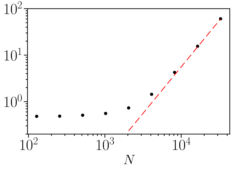
(a) GPU’s memory usage as functions of resolution.

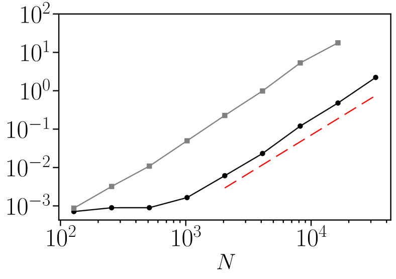
(b) Mean elapsed time as functions of the resolution.

Figure 6: Memory and performance tests for the 4th-order RK temporal scheme. The mean elapsed time is computed as the total physical time to simulate $M$ steps divided by $M$. The CPU comparison test used a similar openMP code with the MKL-FFT library on 32 32-core processor. The red dashed line represents quadratic scaling.

The left panel of Figure 2 shows the total GPU memory usage in Gb (circles) as a function of the resolution $N$. For moderate resolution $N\lesssim 2000$ the memory usage is almost independent of the resolution since most of the memory is used to store the libraries, the kernel, and the resolution-independent variables. For larger resolutions, the memory used to store the 2D fields dominates and therefore it is proportional to $N^{2}$. Remarkably, we observe a similar behavior for the mean elapsed time. This can be explained by the relative smallness of the problem compared to the GPU parallelization capacity. Indeed, not all the registers on the GPUs are required to fully parallelize the computation which therefore is performed in a time independent of the resolution. For larger resolution, the computational time grows proportionally to the amount of computation required for the time step, i.e. to $N^{2}$.

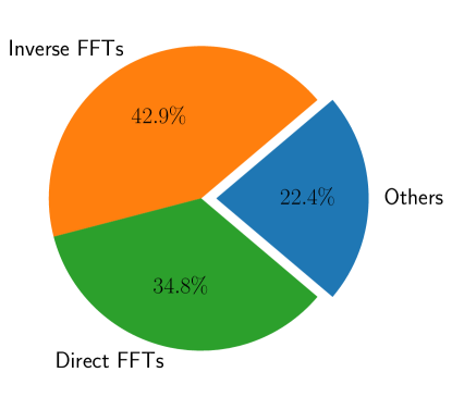
Figure 7: Representative graph of the time spent on the main steps of the time integration.

Figure 7 shows the percentage of time spent on each step of the time integration, step 7 was not included since it is a simple repetition of steps 1 to 6. One should note that the most computationally intensive part is due to the forward and backward FFTs (steps 2 and 4) that account for more than $75\%$ of the computational time. However, the importance of the forward and backward transforms is different since their subroutines are called with different frequencies. Besides, we decided to move the normalization to the forward transform since it has fewer calls per timestep. Although the integrator stability depends intrinsically on the physical properties of the system in question, we observed some practical advantages of using RK4EL in some tested cases. For $\alpha=1$, the governing equations represent a model known as the Surface Quasi Geostrophic (SQG) model [30, 41], which has important applications on atmospheric [27] and ocean flows [2]. On the one hand, the RK2EL scheme is roughly twice as fast as RK4EL since it requires half the number of repetitions. On the other hand, for $N=8192$, we were able to increase the timestep by a factor of almost 5 using the fourth-order scheme. For a simulation with fixed physical time $T=N_{t}dt$, one can have a speedup of approximately $2.5$ on the total simulation time.

References

- Klein et al. [2008] P. Klein, B. L. Hua, G. Lapeyre, X. Capet, S. Le Gentil, and H. Sasaki, Upper ocean turbulence from high-resolution 3d simulations, Journal of Physical Oceanography 38, 1748 (2008).
- Siegelman et al. [2022] L. Siegelman, P. Klein, A. P. Ingersoll, S. P. Ewald, W. R. Young, A. Bracco, A. Mura, A. Adriani, D. Grassi, C. Plainaki, et al., Moist convection drives an upscale energy transfer at jovian high latitudes, Nature Physics 18, 357 (2022).
- Elmegreen and Scalo [2004] B. G. Elmegreen and J. Scalo, Interstellar turbulence i: observations and processes, Annu. Rev. Astron. Astrophys. 42, 211 (2004).
- Frisch [1995] U. Frisch, Turbulence: the legacy of A.N. Kolmogorov (Cambridge University Press, 1995).
- Canuto et al. [1988] C. Canuto, M. Hussaini, A. Quarteroni, and T. Zang, Spectral Methods in Fluid Dynamics, Tech. Rep. (Springer, 1988).
- Boyd [2001] J. P. Boyd, Chebyshev and Fourier spectral methods (Courier Corporation, 2001).
- Mininni et al. [2011] P. D. Mininni, D. Rosenberg, R. Reddy, and A. Pouquet, A hybrid mpi–openmp scheme for scalable parallel pseudospectral computations for fluid turbulence, Parallel computing 37, 316 (2011).
- Lee et al. [2013] M. Lee, N. Malaya, and R. D. Moser, Petascale direct numerical simulation of turbulent channel flow on up to 786k cores, in Proceedings of the International Conference on High Performance Computing, Networking, Storage and Analysis (2013) pp. 1–11.
- Plimpton et al. [2018] S. Plimpton, A. Kohlmeyer, P. Coffman, and P. Blood, fftMPI, a library for performing 2d and 3d FFTs in parallel, Tech. Rep. (Sandia National Lab.(SNL-NM), Albuquerque, NM (United States), 2018).
- Ravikumar et al. [2019] K. Ravikumar, D. Appelhans, and P. Yeung, Gpu acceleration of extreme scale pseudo-spectral simulations of turbulence using asynchronism, in Proceedings of the International Conference for High Performance Computing, Networking, Storage and Analysis (2019) pp. 1–22.
- Rosenberg et al. [2020] D. Rosenberg, P. D. Mininni, R. Reddy, and A. Pouquet, Gpu parallelization of a hybrid pseudospectral geophysical turbulence framework using cuda, Atmosphere 11, 178 (2020).
- Demmel [2013] J. Demmel, Communication-avoiding algorithms for linear algebra and beyond., in IPDPS (2013) p. 585.
- Ayala et al. [2019] A. Ayala, S. Tomov, X. Luo, H. Shaeik, A. Haidar, G. Bosilca, and J. Dongarra, Impacts of multi-gpu mpi collective communications on large fft computation, in 2019 IEEE/ACM Workshop on Exascale MPI (ExaMPI) (IEEE, 2019) pp. 12–18.
- [14] P. Yeung, K. Ravikumar, S. Nichols, and R. Uma-Vaideswaran, Gpu-enabled extreme-scale turbulence simulations: Fourier pseudo-spectral algorithms at the exascale using openmp offloading, Available at SSRN 4821494 .
- Pierrehumbert et al. [1994] R. T. Pierrehumbert, I. M. Held, and K. L. Swanson, Spectra of local and nonlocal two-dimensional turbulence, Chaos, Solitons & Fractals 4, 1111 (1994).
- Xia et al. [2009] H. Xia, M. Shats, and G. Falkovich, Spectrally condensed turbulence in thin layers, Physics of Fluids 21 (2009).
- Benavides and Alexakis [2017] S. J. Benavides and A. Alexakis, Critical transitions in thin layer turbulence, Journal of Fluid Mechanics 822, 364 (2017).
- Musacchio and Boffetta [2017] S. Musacchio and G. Boffetta, Split energy cascade in turbulent thin fluid layers, Physics of Fluids 29 (2017).
- Musacchio and Boffetta [2019] S. Musacchio and G. Boffetta, Condensate in quasi-two-dimensional turbulence, Physical Review Fluids 4, 022602 (2019).
- Zhu et al. [2023] H.-Y. Zhu, J.-H. Xie, K.-Q. Xia, et al., Circulation in quasi-2d turbulence: Experimental observation of the area rule and bifractality, Physical Review Letters 130, 214001 (2023).
- Deusebio et al. [2014] E. Deusebio, G. Boffetta, E. Lindborg, and S. Musacchio, Dimensional transition in rotating turbulence, Physical Review E 90, 023005 (2014).
- Alexakis and Biferale [2018] A. Alexakis and L. Biferale, Cascades and transitions in turbulent flows, Physics Reports 767, 1 (2018).
- Ivey et al. [2008] G. Ivey, K. Winters, and J. Koseff, Density stratification, turbulence, but how much mixing?, Annu. Rev. Fluid Mech. 40, 169 (2008).
- Del Zanna et al. [2024] L. Del Zanna, S. Landi, L. Serafini, M. Bugli, and E. Papini, A gpu-accelerated modern fortran version of the echo code for relativistic magnetohydrodynamics, Fluids 9, 16 (2024).
- De Vanna et al. [2023] F. De Vanna, F. Avanzi, M. Cogo, S. Sandrin, M. Bettencourt, F. Picano, and E. Benini, Uranos: A gpu accelerated navier-stokes solver for compressible wall-bounded flows, Computer Physics Communications 287, 108717 (2023).
- Juckes [1994] M. Juckes, Quasigeostrophic dynamics of the tropopause, Journal of Atmospheric Sciences 51, 2756 (1994).
- Lapeyre and Klein [2006] G. Lapeyre and P. Klein, Dynamics of the upper oceanic layers in terms of surface quasigeostrophy theory, Journal of physical oceanography 36, 165 (2006).
- Hopfinger [1987] E. Hopfinger, Turbulence in stratified fluids: A review, Journal of Geophysical Research: Oceans 92, 5287 (1987).
- Sommeria [1986] J. Sommeria, Experimental study of the two-dimensional inverse energy cascade in a square box, Journal of fluid mechanics 170, 139 (1986).
- Salmon [1998] R. Salmon, Lectures on geophysical fluid dynamics (Oxford University Press, USA, 1998).
- Rivera and Wu [2000] M. Rivera and X.-L. Wu, External dissipation in driven two-dimensional turbulence, Physical review letters 85, 976 (2000).
- Kolmogorov [1941] A. N. Kolmogorov, Equations of turbulent motion in an incompressible fluid, in Dokl. Akad. Nauk SSSR, Vol. 30 (1941) pp. 299–303.
- Onsager [1949] L. Onsager, Statistical hydrodynamics, Il Nuovo Cimento (1943-1954) 6, 279 (1949).
- Bos [2021] W. J. Bos, Three-dimensional turbulence without vortex stretching, Journal of Fluid Mechanics 915, A121 (2021).
- Boffetta and Ecke [2012] G. Boffetta and R. E. Ecke, Two-dimensional turbulence, Annual review of fluid mechanics 44, 427 (2012).
- Kraichnan [1971] R. H. Kraichnan, Inertial-range transfer in two-and three-dimensional turbulence, Journal of Fluid Mechanics 47, 525 (1971).
- Boffetta et al. [2002] G. Boffetta, A. Celani, S. Musacchio, and M. Vergassola, Intermittency in two-dimensional ekman-navier-stokes turbulence, Physical Review E 66, 026304 (2002).
- Haugen and Brandenburg [2004] N. E. L. Haugen and A. Brandenburg, Inertial range scaling in numerical turbulence with hyperviscosity, Physical Review E 70, 026405 (2004).
- Frisch et al. [2008] U. Frisch, S. Kurien, R. Pandit, W. Pauls, S. S. Ray, A. Wirth, and J.-Z. Zhu, Hyperviscosity, galerkin truncation, and bottlenecks in turbulence, Physical review letters 101, 144501 (2008).
- Nam et al. [2000] K. Nam, E. Ott, T. M. Antonsen Jr, and P. N. Guzdar, Lagrangian chaos and the effect of drag on the enstrophy cascade in two-dimensional turbulence, Physical review letters 84, 5134 (2000).
- Blumen [1978] W. Blumen, Uniform potential vorticity flow: Part i. theory of wave interactions and two-dimensional turbulence, Journal of the Atmospheric Sciences 35, 774 (1978).
- Kraichnan [1994] R. H. Kraichnan, Anomalous scaling of a randomly advected passive scalar, Physical review letters 72, 1016 (1994).
- Chertkov [1998] M. Chertkov, On how a joint interaction of two innocent partners (smooth advection and linear damping) produces a strong intermittency, Physics of Fluids 10, 3017 (1998).
- Nam et al. [1999] K. Nam, T. M. Antonsen Jr, P. N. Guzdar, and E. Ott, k spectrum of finite lifetime passive scalars in lagrangian chaotic fluid flows, Physical Review Letters 83, 3426 (1999).
- Dembo [2009] A. Dembo, Large deviations techniques and applications (Springer, 2009).
- Ott [2002] E. Ott, Chaos in dynamical systems (Cambridge university press, 2002).
- Valadão et al. [2024] V. Valadão, T. Ceccotti, G. Boffetta, and S. Musacchio, Non-equilibrium fluctuations of the direct cascade in surface quasi geostrophic turbulence, arXiv e-prints , arXiv (2024).
*