Correlation functions of the Kitaev model with a
spatially modulated phase in the superconducting order parameter

Abstract

The Kitaev model with a spatially modulated phase in the superconducting order parameter exhibits two types of topological transitions, namely a band topology transition between trivial and topological gapped phases, and a Fermi surface Lifshitz transition from a gapped to a gapless superconducting state. We investigate the correlation functions of the model for arbitrary values of superconducting coupling $\Delta_{0}$, chemical potential $\mu$, and phase modulation wavevector $Q$, characterizing the current flowing through the system. In the cases $\mu=0$ or $Q=\pm\pi/2$ correlations are proven to exhibit an even/odd effect as a function of the distance $l$ between two lattice sites, as they are non-vanishing or strictly vanishing depending on the parity of $l$. We identify a clear difference between the two types of transitions through the $Q$-dependence of the short distance correlation functions. In particular, they exhibit pronounced cusps with discontinuous derivatives across the Lifshitz transition. We also determine the long distance behavior of correlations, finding various types of exponential decays in the gapped phase, and an algebraic decay characterized by two different spatial periods in the gapless phase. Furthermore, we establish a connection between the gapless superconducting phase of the Kitaev model and the chiral phase of spin models with Dzyaloshinskii-Moriya interaction.

I Introduction

Correlation functions are one of the most powerful tools to characterize the properties of quantum systems. In topological phase transitions, which cannot be directly signaled by the onset of a spontaneously broken local order parameter [1, 2, 3], their role becomes particularly important. In topological insulators [4, 5, 6], for instance, topological indices can be extracted from the ground-state correlation functions, given on any system portion of the order of the correlation length [7]. In inversion-symmetric Dirac models, correlation functions are closely connected to the Fourier component of the Berry connection (in 1D) and of the Berry curvature (in 2D)  [8, 9]. Also, quantities like entanglement entropy, fidelity and discord, borrowed from quantum information theory and harnessed for detecting topological quantum phase transitions [10, 11, 12, 13], ultimately require the evaluation of correlations. Moreover, single-particle correlation functions of non-interacting systems can be used as a training set in machine learning techniques to predict topological phases of interacting systems [14].

One of the most interesting and widely studied topological quantum systems is the Kitaev model [15], which effectively captures the essential properties of a $p$-wave topological superconductor. The ground state of the model is characterized by two topologically distinct gapped phases and, in the topological non-trivial phase, it exhibits two Majorana quasi-particle (MQP) edge states, whose braiding properties could offer the opportunity to realize topologically protected quantum information [16, 17, 18, 19, 20, 21, 22]. For this reason, various implementations of the 1D Kitaev model have been proposed, based on quantum spin Hall edge states contacted to ferromagnets [23, 24], proximized spin-orbit nanowires [25, 26], ferromagnetic atom chains [27, 28, 29, 30, 31, 32], and cold atoms in optical lattices [33, 34, 35], receiving promising, although not yet conclusive, support from experiments [36, 37, 38, 39, 40, 41, 42, 43, 44]

So far, most studies of the correlation functions in the Kitaev model have focussed on two aspects. Firstly, the analysis of edge correlations in the case of 1D and 2D lattices with open boundary conditions, with the purpose of finding a hallmark of the topological transition between the two gapped phases [45, 46, 47, 48]. Second, the effect of long-ranged hopping and superconducting terms, which do not allow for the customary topological classification. These terms can lead to an algebraic decay of correlation functions even in gapped phases [49, 50, 51, 52] and their realization in ultracold atom setups has been proposed [35].

However, in the experiments conducted on superconductor/semiconducting nanowire setups, where signatures of MQS are often searched for in the zero bias conductance peaks, an electrical current flow is driven across the system. This has recently motivated research groups to investigate the effects of a spatial modulation in the phase of the superconducting order parameter of the Kitaev model [53, 54, 55], where the wavevector $Q$ is related to the net momentum of a Cooper pair, and is non vanishing in the presence of a current flow. In particular, in the regime $\Delta_{0}>w$, where the magnitude $\Delta_{0}$ of the superconducting order parameter is larger than the bandwidth parameter $w$, it has been shown that the spatial modulation wavector $Q$ reduces the boundaries of the topological phase. Additionally, correlation functions have been found to exhibit off-diagonal long-range order at specific parameter points [54]. A recent study has shown that, in the more realistic regime $\Delta_{0}<w$, an even richer scenario arises: Two types of transitions can occur as a function of $Q$ [55]. The first one is related to the band topology and is the customary topological transition between the two gapped phases, while the second one is related to the Fermi surface topology, and is a Lifshitz transition [56, 57] between a gapped and a gapless superconducting phase, which further reduces the parameter range of observability of MQPs [55]. Furthermore, by treating $Q$ as the the wavevector of an extra synthetic dimension, such a Lifshitz transition in the 1D Kitaev model can also be seen as a transition between a type-I to type-II 2D Weyl semimetal.

Motivated by such insightful results, in this work we investigate the correlation functions of the 1D Kitaev model in the presence of the $Q$-modulation in the superconducting parameter phase, considering arbitrary values of the model parameters and of the distance $l$ between the lattice sites of the Kitaev chain. We shall identify the behavior of the correlation functions across the Lifshitz transition and highlight the differences from the more conventional band topology transition between the two gapped phases, at both short and long distances $l$.

The article is structured as follows. In Sec. II we describe the model and summarize those aspects of Ref.[55] that are needed for the present analysis. Then, in Section III we introduce the normal and anomalous correlation functions that we investigate, $\mathcal{C}(l)$ and $\mathcal{A}(l)$ respectively, illustrating the way $Q$ affects their behavior. Moreover, we present our first result: For some noteworthy cases, namely for $\mu=0$ or for $Q=\pm\pi/2$, the correlation functions $\mathcal{C}(l)$ and $\mathcal{A}(l)$ exhibit an even/odd effect, i.e. they are non vanishing or vanishing depending on the parity of the site distance $l$. In Sec.IV we relax such parameter constraints, and analyze the behavior of $\mathcal{C}(l)$ and $\mathcal{A}(l)$ for short distances ($l=1,2$) as a function of the system parameters. We show that their behavior as a function of $Q$ when crossing the Lifshitz transition line from gapped to gapless superconductor phase is quite different from the case of the customary transition from topological to trivial gapped phases. Section V focusses instead on the long distance behavior ($l\gg 1$), and we determine the asymptotic behavior both in the gapped and in the gapless phases. Furthermore, in Sec.IV we discuss the relation between the Kitaev model with superconducting modulation $Q$ and the XY spin model characterized by Dzyaloshinskii-Moriya interaction, highlighting a link in terms of correlation functions between a gapless superconductor and a spin chiral phase. Finally, we summarize our results and draw our conclusions in Sec. VII.

II Model, excitation spectrum and current carrying state

In order to model a 1D $p$-wave TS crossed by a current flow, we include a spatial modulation in the phase of the superconducting order parameter of the Kitaev model, and consider the following Hamiltonian on a 1D lattice

$$\begin{split}\mathcal{H}=&\sum_{j}\left\{w\left(c^{\dagger}_{j}c_{j+1}+c^{\dagger}_{j+1}c_{j}\right)-\mu\left(c^{\dagger}_{j}c_{j}-\frac{1}{2}\right)+\right.\\ +&\left.\Delta_{0}\left(e^{-iQ\left(2j+1\right)}c^{\dagger}_{j}c^{\dagger}_{j+1}+e^{iQ\left(2j+1\right)}c_{j+1}c_{j}\right)\right\}\quad.\end{split}$$ (1)

Here, $c_{j}\,(c^{\dagger}_{j})$ corresponds to the annihilation (creation) operator at the lattice site $j$, while $w>0$ denotes the tunneling amplitude of the hopping term determining the bare bandwidth $4w$, and $\mu$ is the chemical potential. Moreover, the second line of Eq.(1) represents the superconducting term, with $\Delta_{0}>0$ denoting the superconducting coupling, and $Q$ the spatial modulation of its phase, related to the finite momentum $-2Q$ of a Cooper pair in the presence of a current flow. Assuming an infinitely long chain, where the number of sites is $N_{s}\gg 1$, we can adopt periodic boundary conditions (PBCs), and treat $Q$ as a continuum variable.

While details about the model Eq.(1) can be found in Ref.[55], here we shall briefly recall the essential aspects that are needed to discuss how $Q$ affects the normal and the anomalous correlation functions. By applying the Fourier transform and by introducing the Nambu spinors $\Psi_{k;Q}=(c^{\dagger}_{k-Q}\,\,,c_{-k-Q})^{T}$, the Hamiltonian (1) can be rewritten as $\mathcal{H}=\frac{1}{2}\sum_{k}\Psi^{\dagger}_{k;Q}H(k;Q)\Psi_{k;Q}$, where

$$H\left(k;Q\right)=h_{0}(k;Q)\sigma_{0}+\bm{h}\left(k;Q\right)\cdot\bm{\sigma}$$ (2)

is the Bogolubov-de Gennes (BdG) Hamiltonian, ${\bm{\sigma}}=\left(\sigma^{x},\sigma^{y},\sigma^{z}\right)$ denote the Pauli matrices, $\sigma_{0}$ the $2\times 2$ identity,

$$h_{0}(k;Q) = 2w\sin{k}\,\sin{Q}$$ (3)

$${\bm{h}}(k;Q) = (0,\,-\text{Im}\left\{\Delta(k)\right\},\,\xi(k;Q))\quad,$$ (4)

with

$$\xi(k;Q) = 2w\cos{Q}\,\cos{k}\,-\mu$$ (5)

$$\Delta(k) = 2\Delta_{0}i\sin{k}\quad.$$ (6)

Denoting $h(k;Q)=\left|{\bm{h}}(k;Q)\right|=\left[\xi^{2}(k;Q)+\left|\Delta(k)\right|\right]^{1/2}$, the spectrum of the single-particle eigenvalues of the BdG Hamiltonian Eq.(2) reads

$$E_{\pm}(k;Q)=h_{0}(k;Q)\pm h(k;Q)\quad,$$ (7)

where the two bands fulfill the mutual relation

$$E_{-}(k;Q)=-E_{+}(-k;Q)\quad,$$ (8)

stemming from the redundancy of degrees of freedom in the Nambu formalism. Moreover, the eigenvectors $(u_{Q}(k),v_{Q}(k))^{T}$ and $(-v^{*}_{Q}(k),u_{Q}(k))^{T}$ of Eq.(2), where

$$\begin{split}u_{Q}(k)=&\sqrt{\frac{1}{2}\left(1+\frac{\xi(k;Q)}{h(k;Q)}\right)},\\ v_{Q}(k)=&-i\,\text{sgn}\left(\sin(k)\right)\sqrt{\frac{1}{2}\left(1-\frac{\xi(k;Q)}{h(k;Q)}\right)}\end{split}\quad,$$ (9)

enable one to rewrite the Hamiltonian Eq.(1) into its diagonal form

$$\mathcal{H}=\sum_{k}E_{+}(k;Q)\left(\gamma^{\dagger}_{k-Q}\gamma_{k-Q}-\frac{1}{2}\right)$$ (10)

in terms of the Bogolubov quasiparticles,

$$\begin{split}\gamma_{k-Q}=&u_{Q}(k)c_{k-Q}+v_{Q}^{*}(k)c^{\dagger}_{-k-Q}\\ \gamma^{\dagger}_{-k-Q}=&-v_{Q}(k)c_{k-Q}+u_{Q}(k)c^{\dagger}_{-k-Q}\end{split}.$$ (11)

The two terms appearing in the spectrum Eq.(7) allow us to highlight the twofold effect of the superconducting modulation wavevector $Q$. On the one hand, $Q$ renormalizes the bare tunneling amplitude $w\rightarrow w\cos{Q}$ [see Eq.(5)] that appears in the term $h(k;Q)$ of the spectrum Eq.(7). On the other hand, $Q$ introduces in Eq.(7) the $h_{0}$-term Eq.(3), which is not present in the standard Kitaev model ($Q=0$). The first effect alters the boundaries between the topological and trivial gapped phases [54], whereas the second effect can have even more dramatic consequences. Indeed $h_{0}(k;Q)$ breaks the symmetry for $k\rightarrow-k$ of the spectrum and, when its magnitude overcomes $h(k;Q)$ for some $k$’s, it leads to $E_{+}(k;Q)<0$. Importantly, this alters the occupancy of the $E_{+}$ band and the nature of the many-particle ground state [58, 55]. Indeed, Eq.(10) implies that, depending on whether $E_{+}(k;Q)>0$ or $E_{+}(k;Q)<0$, it is energetically more favorable for the system to have the $k$-state empty or occupied. For these reasons, differently from the customary Kitaev model ($Q=0$), where the lower band $E_{-}$ is completely filled, or equivalently the upper band $E_{+}$ is completely empty, the presence of the superconducting modulation can induce an indirect closing of the gap and lead the system to a gapless ground state $\ket{G(Q)}$ of the model (1). As discussed in details in Ref.[55], such ground state can be expressed in general as

$$\ket{G(Q)}=\!\!\prod_{\begin{subarray}{c}0<k<\pi\\ k\in S_{p}\end{subarray}}\!\!\left(u_{Q}(k)+v^{*}_{Q}(k)c^{\dagger}_{-k-Q}c^{\dagger}_{k-Q}\right)\prod_{k\in S_{e}}c^{\dagger}_{k-Q}\ket{0},$$ (12)

where the Brillouin zone (BZ) gets decomposed in three sectors, ${\rm BZ}=S_{p}\cup S_{e}\cup S_{h}$, identified through the three possible values

$$\eta(k;Q)=\left\{\begin{array}[]{cc}1&k\in S_{h}\\ 0&k\in S_{p}\\ -1&k\in S_{e}\end{array}\right..$$ (13)

of the spectral asymmetry function

$$\eta(k;Q)=\frac{1}{2}\left\{\text{sgn}E_{+}(k;Q)+\text{sgn}E_{-}(k;Q)\right\}\quad.$$ (14)

The sector $S_{p}$ represents the pair sector, as it involves in the ground state Eq.(12) Cooper pairs with a total momentum $-2Q$, while $S_{e}$ represents the unpaired electron sector, since only single electrons appear in Eq.(12) for $k\in S_{e}$, and $S_{h}$ is the unpaired hole sector, since no electron state appears in Eq.(12) for $k\in S_{h}$. Note that, as a consequence of Eq.(8), the unpaired hole sector $S_{h}$ can be seen as the mirror of the unpaired electron sector $S_{e}$ under $k\rightarrow-k$, while the pair sector $S_{p}$ is self-mirrored under such transformation.

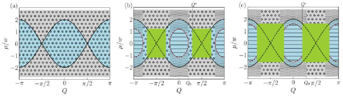
Figure 1: Phase diagram of the Kitaev model as a function of the wavevector $Q$ (spatial modulation of the superconducting order parameter) and chemical potential $\mu$, for three different values of the superconducting coupling: (a) $\Delta_{0}=1.3w$; (b) $\Delta_{0}=0.8w$; (c) $\Delta_{0}=0.6w$. Grey and cyan areas denote the trivial and topological gapped phases, respectively, while the green region denotes the gapless superconducting phase. Different symbols in the gapped phases identify three different types of exponential decay in the correlation functions, at long distance $l\gg 1$. In regions marked with “$\circ$”, and “$\cdot$”, the correlations decay as Eqs.(35)-(36) and Eqs.(59)-(60), respectively, while inside the elliptic region “$-$” they decay as Eqs.(67)-(68). Inside the gapless phase correlations decay algebraically as Eqs.(V.0.2)-(V.0.2). The crossing between situations (b) and (c), where the elliptic gapped region and the gapless region touch, occurs at the value $\Delta_{0}^{*}=w/\sqrt{2}$. The wavevector $Q^{*}$, given in Eq.(71), identifies the gapped/gapless boundary, while $Q_{0}$, given in Eq.(72), determines the boundary between the “$\circ$” and “$\cdot$” regions.

The ground state of the system can be in two possible type of phases.

Gapped phase. The gapped phase is characterized by the condition $E_{+}(k;Q)>0\,\,\forall k\in{\rm BZ}$, which in turn implies $E_{-}(k;Q)<0\,\,\forall k\in{\rm BZ}$, on account of Eq.(8). Then, Eq.(14) implies $\eta(k;Q)\equiv 0\,\,\,\forall k\in{\rm BZ}$, and from Eq.(13) one deduces that the pair sector $S_{p}$ covers the entire Brillouin zone, leaving the $S_{e}$ and $S_{h}$ sectors empty

$$\begin{array}[]{l}S_{p}\equiv{\rm BZ}\leftrightarrow k\in[-\pi,\pi]\\ \\ S_{e}=S_{h}=\emptyset\end{array}\quad.$$ (15)

In this case, the general expression (12) of the ground state reduces to the standard form consisting of Cooper pairs only. The gapped phase occurs if and only if one of the following three parameter conditions is fulfilled[55]

$$\begin{array}[]{lcl}i)&|\mu|>2w\mbox{ \& }&\forall\Delta_{0}>0\mbox{ \& }\forall Q\\ ii)&|\mu|<2w\mbox{ \&}&\sqrt{w^{2}-\mu^{2}/4}<\Delta_{0}\,\mbox{ \& }\left|\cos{Q}\right|\neq|\mu|/2w\\ iii)&|\mu|<2w\mbox{ \& }&w|\sin{Q}|<\Delta_{0}<\sqrt{w^{2}-\mu^{2}/4}\end{array}.$$ (16)

As is well known, there exist two topological distinct gapped phases, separated by the curves $\left|\mu\right|=2w\left|\cos{Q}\right|$ in the parameter space, where the gap in the excitation spectrum closes directly at either $k^{*}=0$ or $k^{*}=\pi$, i.e. when $E_{+}(k^{*};Q)=E_{-}(k^{*};Q)=0$.

Gapless phase. When, however, $E_{+}(k;Q)<0$ for some $k$, the gap between the two bands closes indirectly since $E_{-}(-k;Q)>0$. In this case Eq.(13) implies that the unpaired electron sector $S_{e}$ is not an empty set, just like its $k$-mirror set $S_{h}$. Cooper pairs are present only in a portion $S_{p}$ of the Brillouin zone and the ground state is strictly mixed, as given by Eq.(12). Such type of state arises also in other contexts, such as $s$-wave paired superfluids with rotationally symmetric confinement potentials [59, 60] and Fermi gases with two species of Fermions [61]. The ground state of model (1) is in the gapless phase when both the following conditions are fulfilled[55]

$$\sqrt{\Delta_{0}^{2}+\frac{\mu^{2}}{4}}<w\,\,\,\&\,\,\,\Delta_{0}<w|\sin{Q}|\quad.$$ (17)

In particular, one can show that the unpaired fermions (electron or holes) sector $S_{u}=S_{e}+S_{h}$ of the Brillouin zone is given by

$$\begin{array}[]{c}S_{u}\,\,=\left\{\,\,k\,\,|\,\,\left|k^{*}_{-}\right|<\left|k\right|<\pi-\left|k^{*}_{+}\right|\right\}\end{array}$$ (18)

while the pair sector is

$$S_{p}=\left\{k\,\,|\,\,0<|k|<|k^{*}_{-}|\,\,\mbox{or}\,\,\pi-\left|k^{*}_{+}\right|<\left|k\right|<\pi\right\}\quad.$$ (19)

where

$$k^{*}_{\pm}=\arcsin\left(\frac{\cos{Q}}{\sqrt{1-\frac{\Delta^{2}_{0}}{w^{2}}}}\right)\pm\arcsin\left(\frac{\mu}{2w\sqrt{1-\frac{\Delta^{2}_{0}}{w^{2}}}}\right).$$ (20)

We conclude this section by recalling the phase diagram of the Kitaev model (1), obtained in Ref.[55]. Here it is shown in Fig.1 as a function of the superconducting modulation wavevector $Q$ and the chemical potential $\mu$, for three different values of $\Delta_{0}$. Here cyan and gray areas denote the topological and trivial gapped phases, respectively, while the green area denotes the gapless region. While for $\Delta_{0}>w$ only the gapped phase exists [panel (a)], and the ground state only consists of Cooper pairs, for the physically realistic regime $\Delta_{0}<w$ also the gapless phase appears. It exists for parameter values (17), and is the more extended the lower the values of $\Delta_{0}$ [panels (b) to (c)]. The additional symbols appearing in Fig.1 identify different long distance behavior of the correlation functions, as we shall explain in detail in Sec.V.

III Correlation functions: expressions and even/odd effect

We now determine the real-space behavior of the correlation functions of the model (1). Specifically, we shall consider the normal and the anomalous correlation, defined as

$$\mathcal{C}(l) = e^{iQl}\langle c^{\dagger}_{j}c_{j+l}\rangle$$ (21)

$$\mathcal{A}(l) = e^{-iQ(2j+l)}\langle c^{\dagger}_{j}c^{\dagger}_{j+l}\rangle\quad,$$ (22)

respectively. Here the expectation values $\langle\cdots\rangle$ are computed with respect to the ground state $\ket{G(Q)}$, whose general expression is given by Eq.(12). Due the translational invariance of the model, $\mathcal{C}$ and $\mathcal{A}$ only depend on the site distance $l$, which is assumed to be $l\neq 0$, and are independent of the site $j$. Straightforward algebra, whose details are given in Appendix A, enables one to re-express the correlations Eqs.(21)-(22) as integrals in momentum space, and to identify the different contributions related to the sector $S_{p}$, $S_{e}$, $S_{h}$ characterizing the ground state (12). Specifically, one finds

$$\mathcal{C}(l)=\mathcal{C}_{p}(l)+i\,\mathcal{C}_{u}(l)\,,$$ (23)

where

$$\mathcal{C}_{p}(l)=-\frac{1}{4\pi}\intop_{S_{p}}dk\frac{\cos(kl)\xi(k;Q)}{h(k;Q)}$$ (24)

represents the Cooper pair contribution, and is the real part of $\mathcal{C}(l)$, whereas

$$\mathcal{C}_{u}(l) = \frac{1}{2\pi}\intop_{S_{e}}dk\sin(kl)$$ (25)

represents the unpaired electron contribution, and is the imaginary part of $\mathcal{C}(l)$. Similarly, the anomalous correlation function can be re-expressed as

$$\mathcal{A}(l)=-\frac{\Delta_{0}}{2\pi}\intop_{S_{p}}dk\frac{\sin(kl)\sin{k}}{h(k;Q)},\,\,$$ (26)

and only consists of contributions from Cooper pairs, as expected.

A comment is in order about how $Q$ enters the expressions Eqs.(24)-(25) and (26) of the correlation functions. On the one hand, the integrand functions in these equations depend on $Q$ only through the effect of renormalization $w\rightarrow w\cos{Q}$ of the tunneling amplitude, encoded in the functions $h(k;Q)$ and $\xi(k;Q)$. On the other hand, the integration domains $S_{p}$ and $S_{e}$, which are determined by the spectral asymmetry values Eq.(13), also depend on the $h_{0}(k;Q)$ term of the spectrum Eq.(7), which is responsible for the possible change induced by $Q$ in the band occupancy.

Let us now turn to the evaluation of the correlation functions Eqs.(24)-(25) and (26). Firstly, we note that the unpaired fermion contribution $\mathcal{C}_{u}$ can be given an analytical exact expression for arbitrary parameter values. Indeed, in the gapped phase, the spectral asymmetry always vanishes, $\eta\equiv 0\,\,\forall k\in{\rm BZ}$ [see Eq.(13)], and one has $\mathcal{C}_{u}=0$. In contrast, in the gapless phase, one can rewrite Eq.(25) as

$$\mathcal{C}_{u}(l) = -\frac{1}{4\pi}\intop_{S_{u}}dk\sin(kl)\eta(k;Q)=$$ (27)

$$= -\frac{\text{sgn}(Q)}{2\pi}\frac{1}{l}\left(\cos(k^{*}_{-}l)-(-1)^{l}\cos(k^{*}_{+}l)\right)\quad,$$

where $k^{*}_{\pm}$ are given in Eq.(20) and Eqs.(13) and (18) have been used. For the Cooper pair contributions $\mathcal{C}_{p}(l)$ to the normal correlator, and for the anomalous correlator $\mathcal{A}(l)$, analytical results are not available in general. Nevertheless, we can obtain such correlations by numerically exact integration of Eqs.(24) and (26) and, in some limits, we can provide analytical expressions. Here and in the next sections we shall present these results, pointing out the effect of the $Q$-wavevector related to the current flow.

III.1 Even/odd effect for the special cases
$\mu=0$ or $Q=\pm\pi/2$

We start by discussing two noteworthy cases, namely $\mu=0$ and $Q=\pm\pi/2$, where the correlation functions can be rigorously shown to exhibit an even/odd effect. Indeed $\mathcal{C}(l)$ and $\mathcal{A}(l)$ are non-vanishing or vanishing depending on the even/odd parity of the site distance $l$. This result, whose demonstration is given in Appendix B, is summarized in Tables 1 and 2.

Specifically, Table 1 refers to the case $\mu=0$ and shows that both the normal and the anomalous correlation functions vanish at any even site distance $l$, for any value of $Q$ and $\Delta_{0}$. It thus holds both in the gapped and in the gapless phase, although the decay of correlations for $l\gg 1$ is different in the two phases, as we shall discuss in details in Sec.V. An example of even/odd effect is shown in Fig.2(a), where $\mathcal{C}$ at $\mu=0$ is plotted as a function of $l$ for $\Delta_{0}=1.3w$, $Q=0.6\pi$.

Table 2 illustrates the case $Q=\pm\pi/2$. Note that the anomalous correlation $\mathcal{A}$ still vanishes at any even site distance $l$, both in the gapped and in the gapless phase, as also shown by the example plotted in panel (b) of Fig.2 for $\Delta_{0}=0.8w$ and $\mu=0.5w$. However, the normal correlation function $\mathcal{C}$ exhibits a qualitatively different effect depending on the ground state phase. Specifically, in the gapped phase, it strictly vanishes for any odd site distance $l$. However, in the gapless phase $\mathcal{C}(l)$ takes contribution only from Cooper pairs, $\mathcal{C}(l)=\mathcal{C}_{p}(l)$ if $l$ is even, while it purely stems from the unpaired fermion term, $\mathcal{C}(l)=i\mathcal{C}_{u}(l)$ for odd $l$ values.
For small values of distance ($l\leq 3$), it is also possible to find analytical expressions for the (non vanishing) correlations in terms of elliptic functions, which are reported in Appendix B.

	gapped phase	gapless phase
$\mathcal{C}(l)$	$0$	$0$	$l\,\,\text{even}$
	✓	✓	$l\,\,\text{odd}$
$\mathcal{A}(l)$	$0$	$0$	$l\,\,\text{even}$
	✓	✓	$l\,\,\text{odd}$

$(\mu=0)$

Table 1: The case $\mu=0$: Correlation functions for $l\neq 0$. Both the normal and the anomalous correlation function (21) and (22) are strictly vanishing for any even value of the site distance $l\neq 0$, while they are non-vanishing for $l$ odd. This holds both in the gapped and in the gapless phase.

	gapped phase	gapless phase
$\mathcal{C}(l)$	✓	$\equiv\mathcal{C}_{p}(l)$	$l\,\,\text{even}$
	$0$	$\equiv i\mathcal{C}_{u}(l)$	$l\,\,\text{odd}$
$\mathcal{A}(l)$	$0$	$0$	$l\,\,\text{even}$
	✓	✓	$l\,\,\text{odd}$

$(Q=\pm\frac{\pi}{2})$

Table 2: The case $Q=\pm\pi/2$: Correlation functions for $l\neq 0$. While the anomalous correlation function (22) vanishes for any even values of $l$, the normal correlation function exhibits a different behavior depending on whether the system ground state is in its gapped or in the gapless phase. In the former case it strictly vanishes for any odd $l$, while in the latter case it either gets contribution only from Cooper pairs, $\mathcal{C}=\mathcal{C}_{p}$ (for even $l$) or from the unpaired fermions $\mathcal{C}=i\mathcal{C}_{u}$ (for odd $l$).

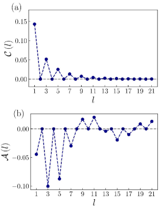
Figure 2: The even/odd effect of the correlation functions. Panel (a) is an example of Table 1 and shows the normal correlation function (21) as a function of $l>0$, for $\mu=0$, $Q=0.6\pi$ and $\Delta_{0}=1.3$ (ground state in the gapped phase). Panel (b) is an example of Table 2 and shows the anomalous correlation (22) as a function of $l>0$, for the values $\mu=0.5$, $Q=\pi/2$ and $\Delta_{0}=0.8$ (ground state in the gapless phase). In both cases the correlation functions vanish exactly at $l$ even.

We conclude this subsection by a comment on the two special points of the parameter space, namely $(Q,\mu)=(\pm\pi/2,0)$, which can be regarded to as the intersection of Tables 1 and 2. These two special points were recently analyzed in Ref.[54], where off-diagonal long range order was found in the correlations in the regime $\Delta_{0}>w$. Because in such regime the system is always in the gapped phase [panel (a) of Fig.1], we also deduce from Tables 1 and 2 that normal correlation at arbitrary site distance $l$ vanishes, $\mathcal{C}(l)\equiv 0\,\,\forall l>0$ (even and odd), and only anomalous correlation exists at such point. Moreover, our results enable to extend the analysis to the regime $\Delta_{0}<w$, where these special points are always in the gapless phase, instead. In this case Tables 1 and 2 predict that the normal correlation is vanishing for even $l$, while for odd $l$ it only gets contribution from the unpaired fermion sector, $\mathcal{C}=i\mathcal{C}_{u}$. As we shall see in Sec.VI, $\mathcal{C}_{u}$ can be related to spin chiral gapless phases in spin models.

IV Short distance behavior of correlation functions

We analyse now the behaviour of the correlation functions (21) and (22) at short distance $l$, for arbitrary values of the parameters $Q$, $\mu$, and $\Delta_{0}$. Specifically, by the numerically exact evaluation of $\mathcal{C}_{p}$ and $\mathcal{A}$ in Eqs.(24) and (26), we shall analyze the quantities $\left|\mathcal{C}(l)\right|^{2}=\mathcal{C}^{2}_{p}(l)+\mathcal{C}^{2}_{u}(l)$ and $\left|\mathcal{A}(l)\right|^{2}$. The former can be considered as the probability for an electron to hop from site $j+l$ to $j$, while the latter corresponds to the probability of creating a Cooper pair at sites $j$ and $j+l$. We shall focus here on the short distance values $l=1$ and $l=2$.

IV.0.1 The case $l=1$

Let us start by analyzing the case $l=1$. The two quantities $\left|\mathcal{C}(1)\right|^{2}$ and $\left|\mathcal{A}(1)\right|^{2}$ are shown in Fig.3 as contour plots over the parameter space $(Q,\mu)$, at a fixed value of $\Delta_{0}$. Specifically, the two upper panels refer to the regime $\Delta_{0}>w$, where the system exhibits only the two topologically different gapped phases [see Fig.1(a)], while the two lower panels of Fig.3 refer to the regime $\Delta_{0}<w$, where the gapless phase appears in the $(Q,\mu)$ parameter space [green areas of Fig.1(c)].

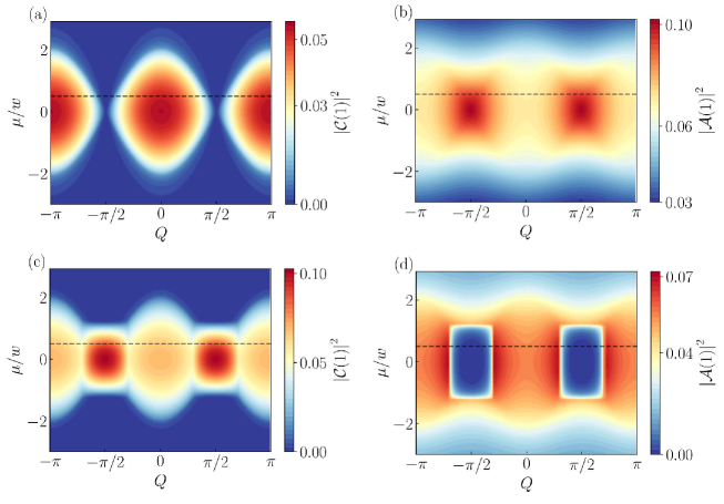
Figure 3: Normal and anomalous correlation functions, Eq.(21) and Eq.(22), for $l=1$. Contour plots of $|\mathcal{C}(1)|^{2}$ and $|\mathcal{A}(1)|^{2}$ as a function of the Cooper pair wavevector $Q$ and chemical potential $\mu$. Panels (a) and (b) are obtained for $\Delta_{0}=1.3w$. The behavior of $|\mathcal{C}(1)|^{2}$ in panel (a) reflects the phase diagram of Fig.1(a) where two topologically distinct gapped phases exist. Panels (c) and (d) are obtained for $\Delta_{0}=0.8w$, and both clearly show the emergence of a gapless region as a sharp rectangular area centered around the special points $(Q,\mu)=(\pm\pi/2,0)$ [green areas of Fig.1(c)]. Horizontal dashed lines identify the cuts at $\mu=0.5w$, shown in Figs.4 and 5.

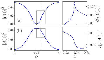
Figure 4: The squared modulus of the normal and anomalous correlations $\mathcal{C}(1)$ and $\mathcal{A}(1)$ are plotted as a function of $Q$, for $\Delta_{0}=1.3w$. (a) and (b) panels represent cuts of Fig.3(a) and Fig.3(b), respectively, at $\mu=0.5w$. Right panels display the $Q$-derivative of the corresponding curve on the left in the range highlighted by rectangles. Vertical dashed lines mark the transition point between the trivial and the topological gapped phases.

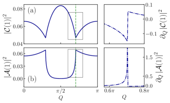
Figure 5: The squared modulus of the normal and anomalous correlations $\mathcal{C}(1)$ and $\mathcal{A}(1)$ are plotted as a function of $Q$, for $\Delta_{0}=0.8w$. (a) and (b) panels represent cuts of Fig.3(c) and Fig.3(d), respectively, at $\mu=0.5w$. Right panels display the $Q$-derivative of the corresponding curve on the left in the range highlighted by rectangles. Vertical dashed lines mark the Lifshitz transition line separating the gapped from the gapless phases.

From Fig.3(a), one can see that the contour plot of the squared normal correlation function $|\mathcal{C}(1)|^{2}$ qualitatively reproduces the phase diagram of Fig.1(a), reaching its maximal values at the center of the gapped topological phase and being suppressed in the trivial gapped phase. Instead, it would be harder to infer such phase diagram from the inspection of the anomalous correlation function $|\mathcal{A}(1)|^{2}$, shown in Fig.3(b). Yet, from such a plot we deduce that the maximal probability of finding nearest neighbors Cooper pairs is at the special points $(Q,\mu)=(\pm\pi/2,0)$, in agreement with the result discussed at the end of Sec.III.1 that all normal correlation functions vanish (at any distance) for such parameter values. Focussing now on the $\Delta_{0}<w$ regime, we observe that both the normal and the anomalous correlation functions depicted in panels (c) and (d) of Fig.3 clearly exhibit a rectangular shape, centered around the special points $(Q,\mu)=(\pm\pi/2,0)$, identifying the gapless region of Fig.1(b). It is straightforward to show that the values of correlations at the special points are

$$\left.\mathcal{C}(1)\right|_{\mu=0;Q=\pm\frac{\pi}{2}} = i\left.\mathcal{C}_{u}(1)\right|_{\mu=0;Q=\pm\frac{\pi}{2}}=$$ (30)

$$= \left\{\begin{array}[]{lcl}0&\mbox{for}&\Delta_{0}>w\\ \pm\frac{i}{\pi}&\mbox{for}&\Delta_{0}<w\\ \end{array}\right.$$

and

$$\left.\mathcal{A}(1)\right|_{\mu=0;Q=\pm\frac{\pi}{2}}=\left\{\begin{array}[]{lcl}0&\mbox{for}&\Delta_{0}>w\\ -\frac{1}{\pi}&\mbox{for}&\Delta_{0}<w\\ \end{array}\right.$$ (31)

The question we now want to address is whether the $Q$-dependence of the correlation functions enables one to distinguish the two types of transitions, namely the band topology transition (from trivial gapped to topological gapped) and the Fermi surface topology Lifshitz transition (gapped to gapless). To this purpose, for each panel in Fig.3, we have analysed a horizontal cut at $\mu=0.5w$. The cuts of the upper panels (a) and (b) of Fig.3 are shown in Fig.4 [panels (a) and (b), respectively] and display the behavior of $|\mathcal{C}(1)|^{2}$ of $|\mathcal{A}(1)|^{2}$ across the band topology transition, occurring at the two values $Q=\arccos(\pm\mu/2w)$. One of them is highlighted as a vertical dashed line. As one can see, the behavior appears to be smooth. To have a closer inspection around the transition point, we have focussed on the $Q$-range enclosed by boxes, and we have depicted the derivatives $\partial_{Q}|\mathcal{C}(1)|^{2}$ and $\partial_{Q}|\mathcal{A}(1)|^{2}$ in the right panels of Fig.4. As one can see, while the anomalous correlation has a finite and continuous derivative, the normal correlation exhibits a divergent derivative at the transition point, related to the direct closing at $k=\pi$ of the gap between the two bands $E_{+}$ and $E_{-}$. Note, however, that the behavior is the same on both sides (trivial and topological) of the transition, in agreement with the universality of the correlation length scaling discussed in Ref.[8].

Let us now analyze the cuts of Fig.3(c) and Fig.3(d), which are shown in panels (a) and (b) of Fig.5, and refer to the Lifshitz transition. We now observe clear cusps appearing both in $|\mathcal{C}(1)|^{2}$ and $\mathcal{A}(1)|^{2}$ at the boundaries between gapped and gapless phases, which are determined by the indirect closing of the gap between the two bands $E_{+}$ and $E_{-}$. The boundary at the value $Q=\pi-\arcsin(\Delta_{0}/w)$ is highlighted by the vertical dashed line, and the related discontinuity in the derivatives is shown by the focus in the right panels of Fig.5. The comparison between Figs.4 and 5 shows the difference in the $Q$-dependence of the correlation functions across the two types of transitions. Due to the presence of cusps, the Lifshitz transition has a much sharper evidence than the band topology transition between gapped phases. The origin of such cusps boils down to the intrinsically different structure of the ground state on the two sides (gapped vs gapless) of the transition, which affects the correlation functions. Indeed, as observed at the beginning of this section, the integral expressions (24) and (26) have a twofold dependence on $Q$, namely through the integrand function and through the integration domain. In the gapped side of the transition only the former is present, since $S_{p}\equiv{\rm BZ}$ is $Q$-independent, whereas in the gapless side also the latter leads to a finite contribution, since $S_{p}$ is given by Eqs.(19)-(20) and depends on $Q$. This gives rise to the discontinuity of the correlation function derivatives $\partial_{Q}|\mathcal{C}(1)|^{2}$ and $\partial_{Q}|\mathcal{A}(1)|^{2}$ shown in the right panels of Fig.5.

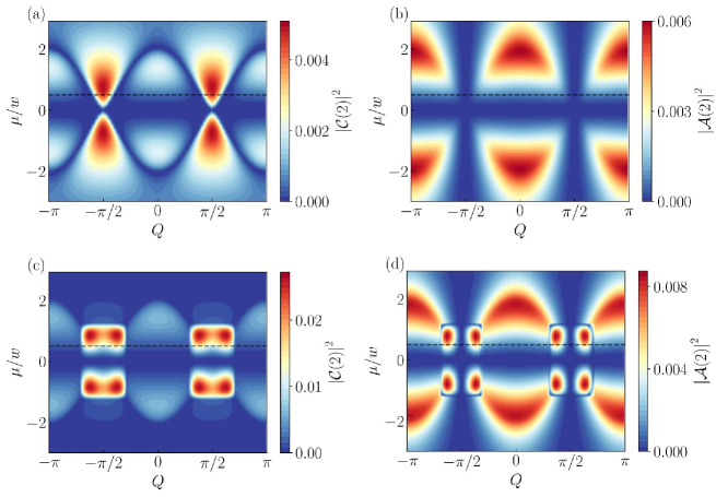
Figure 6: Normal and anomalous correlation functions, Eq.(21) and Eq.(22), for $l=2$. Contour plots of $|\mathcal{C}(2)|^{2}$ and $|\mathcal{A}(2)|^{2}$ as a function of the Cooper pair wavevector $Q$ and chemical potential $\mu$. Panels (a) and (b) are obtained for $\Delta_{0}=1.3w$, while panels (c) and (d) for $\Delta_{0}=0.8w$. The behavior of $|\mathcal{C}(2)|^{2}$ in panel (a) reflects the phase diagram of Fig.1(a), while both $|\mathcal{C}(2)|^{2}$ and $|\mathcal{A}(2)|^{2}$ in panels (c) and (d) acquire some local maxima inside the rectangular region identifying the gapless phase.

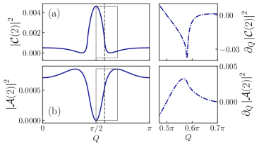
Figure 7: The squared modulus of the normal and anomalous correlations $\mathcal{C}(2)$ and $\mathcal{A}(2)$ are plotted as a function of $Q$, for $\Delta_{0}=1.3w$. (a) and (b) panels represent cuts of Fig.6(a) and Fig.6(b), respectively, at $\mu=0.5w$. Right panels display the $Q$-derivative of the corresponding curve on the left in the range highlighted by rectangles. Vertical dashed lines mark the transition point between the trivial and the topological gapped phases.

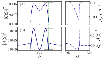
Figure 8: The squared modulus of the normal and anomalous correlations $\mathcal{C}(2)$ and $\mathcal{A}(2)$ are plotted as a function of $Q$, for $\Delta_{0}=0.8w$. (a) and (b) panels represent cuts of Fig.6(c) and Fig.6(d), respectively, at $\mu=0.5w$. Right panels display the $Q$-derivative of the corresponding curve on the left in the range highlighted by rectangles. Vertical dashed lines mark the Lifshitz transition line separating the gapped from the gapless phases.

IV.0.2 The case $l=2$

Let us now consider the probabilities $|\mathcal{C}(2)|^{2}$ and $|\mathcal{A}(2)|^{2}$ related to next nearest neighbor processes of electron hopping or pair production. These are shown in Fig.6 as contour plots, where again the upper panels (a) and (b) correspond to the regime $\Delta_{0}>w$, and the lower panels (c) and (d) to the regime $\Delta_{0}<w$ where the gapless phase appears. A first striking difference between Fig.6 ($l=2$) and Fig.3 ($l=1$) is the even/odd effect, which is schematically described in Tables 1 and 2 and can now be appreciated by inspecting the horizontal line $\mu=0$ and the vertical lines $Q=\pm\pi/2$, respectively. Indeed at $\mu=0$ both $|\mathcal{C}(2)|^{2}$ and $|\mathcal{A}(2)|^{2}$ vanish, in striking contrast with $|\mathcal{C}(1)|^{2}$ and $|\mathcal{A}(1)|^{2}$. For $Q=\pm\pi/2$ one observes that $|\mathcal{A}(2)|^{2}$ vanishes, while $|\mathcal{C}(2)|^{2}$ does not, in agreement with Table 2. Another striking difference is related to the gapless region. While from the $l=1$ correlations shown in Fig.3 the gapless region appears as a uniform rectangular shape, the $l=2$ correlations in Fig.6 reveal an inner structure with local maxima.

Then, similarly to what was done for $l=1$, we have investigated the difference between two types of transitions by analyzing the $Q$ dependence of $|\mathcal{A}(2)|^{2}$ and $|\mathcal{C}(2)|^{2}$. The cuts at $\mu=0.5w$ of the upper panels (a) and (b) of Fig.6 are shown in Fig.7 and are related to the transition between the gapped phases, while the cuts of the lower panels (c) and (d) of Fig. 6 are shown in Fig.8 and highlight the behavior across the Lifshitz transition. The corresponding derivatives around the transition boundaries are shown in the right panels of Figs. 7 and 8. As one can see from Fig.7, $|\mathcal{A}(2)|^{2}$ and $|\mathcal{C}(2)|^{2}$ vary smoothly across the band topology transition, while cusps clearly appear in Fig.8. This means that, despite the above mentioned differences between the $l=1$ and the $l=2$ case, the $Q$ dependence of both cases indicates that the gapped to gapless Lifshitz transition is far more detectable than the band topology transition.

V Long distance behavior of correlation functions

We now turn to evaluate the asymptotic behavior of the normal and anomalous correlations $\mathcal{C}(l)$ and $\mathcal{A}(l)$ at long distance $l\gg 1$. The behavior significantly changes from the gapped to the gapless phase. Moreover, even within the gapped phase, different asymptotic behaviors arise in the regime $\Delta_{0}<w$.

V.0.1 Asymptotic behavior in the gapped phases

In the gapped phase (16), the asymptotic behavior of the correlation functions can be obtained by re-expressing Eqs.(24) and (26) in a different but equivalent form, based on complex analysis. While the technicalities of this procedure are given in the Appendix C, here we briefly illustrate its main steps, which will be useful to elucidate the various asymptotic behaviors that emerge, depending on the parameter ranges.

As observed above, in the gapped phase the unpaired fermion sector $S_{u}$ is an empty set [see Eq.(15)], and the unpaired fermion contribution in Eq.(25) therefore vanishes,

$$\mathcal{C}_{u}=0\quad.$$ (32)

As the ground state only involves Cooper pairs, the pair sector $S_{p}$ coincides with the entire Brillouin zone [see Eq.(15)]. Thus, by interpreting $k\in[-\pi;\pi]$ as the phase of a complex number $z=e^{ik}$ that spans over the unit circle, it is possible to recast the correlation functions in the form of integrals in the complex plane [50, 52]

$$\mathcal{C}_{p}(l) = -\frac{1}{4\pi}\text{Im}\left\{\oint_{\left|z\right|=1}dz\frac{z^{l-1}g\left(z\right)}{\sqrt{g^{2}\left(z\right)-f^{2}\left(z\right)}}\right\}$$ (33)

$$\mathcal{A}(l) = \frac{1}{4\pi}\text{Im}\left\{\oint_{\left|z\right|=1}dz\frac{z^{l-1}f\left(z\right)}{\sqrt{g^{2}\left(z\right)-f^{2}\left(z\right)}}\right\},$$ (34)

where the functions $f(z)=\Delta_{0}(z-z^{-1})$ and $g(z)=w\left(z-z^{-1}\right)\cos{Q}-\mu$ of the complex variable take the values $f(e^{ik})=\Delta(k)$ and $f(e^{ik})=\xi(k;Q)$ over the unit circle $|z|=1$, respectively. The denominator of Eqs.(33)-(34) exhibits four branch points, whose location depends on the specific parameter values $\Delta_{0}$, $Q$ and $\mu$. It is possible to show that two of such branch points, which we shall denote as $z^{*}_{\pm}$, lie inside the unit circle ($|z^{*}_{\pm}|<1$), while the other two lie outside it and are given by $1/z^{*}_{\pm}$. Then, Cauchy theorem applied to Eqs.(33)-(34) enables one to rewrite Eqs.(33)-(34) as contour integrals over the branch cuts connecting the inner branch points $z^{*}_{\pm}$. Thus, it is the location of $z^{*}_{\pm}$ that determines the different asymptotic behavior of the correlation functions for $l\gg 1$. Details are given in the Appendix C

With keeping in mind that here the parameter conditions (16) for the gapped phase are assumed to hold, one can identify three possible configurations for the location of $z^{*}_{\pm}$ in the complex plane, which determine three different types of asymptotic behaviors and are highlighted with different symbols in Fig.1.

$(1)$   $z^{*}_{\pm}$ are real and have opposite signs
When this branch point configuration occurs, the correlation functions decay as

$$\mathcal{C}_{p}(l)\sim -\frac{1}{2\sqrt{l}}\left(\alpha^{+}_{1}e^{-\kappa_{+}l}-\left(-1\right)^{l}\alpha^{-}_{1}e^{-\kappa_{-}l}\right),$$ (35)

$$\mathcal{A}(l)\sim -\frac{1}{2\sqrt{l}}\left(\beta^{+}_{1}e^{-\kappa_{+}l}-\left(-1\right)^{l}\beta^{-}_{1}e^{-\kappa_{-}l}\right),$$ (36)

where

$$\kappa_{\pm}=\ln\frac{1}{\left|z^{*}_{\pm}\right|}$$ (37)

represent the inverse decay lengths, while the constants $\alpha_{1}^{\pm}$ and $\beta_{1}^{\pm}$ depend on $|z^{*}_{\pm}|$ and are explicitly given in Appendix C as a function of the parameter values. Such a configuration of real branch points with opposite signs occurs when the conditions

$$\left\{\begin{array}[]{l}\Delta_{0}^{2}+\frac{\mu^{2}}{4}-w^{2}\cos^{2}{Q}>0\\ \Delta_{0}>w|\cos{Q}|\end{array}\right.$$ (38)

are both fulfilled. For a given $\Delta_{0}$ value, the portions of the $Q$-$\mu$ phase diagram where the gapped phase fulfills the additional conditions (38) and the correlation asymptotic behavior is given by Eqs.(35)-(36) are highlighted as circles “$\circ$” in Fig.1. Note that, in the regime $\Delta_{0}>w$, where for any value of $Q$ and $\mu$ the Kitaev model only exhibits gapped phases (either trivial or topological) [panel (a) of Fig.1], the conditions (38) are fulfilled, whereas for $\Delta_{0}<w$ it only holds in subregions of the phase diagram [panel (b) and (c) of Fig.1].

Various features are noteworthy in the expressions Eqs.(35) and (36). First, they exhibit a combination of two exponential decays that are further enhanced by the additional $1/\sqrt{l}$ factor. Second, the inverse decay lengthscales are determined by the moduli $|z^{*}_{\pm}|$ of the inner branch points Eq.(37). Note that, because the inner branch points $z^{*}_{\pm}$ have opposite signs, the magnitude of $|z^{*}_{+}|$ and $|z^{*}_{-}|$ might be comparable, and both the exponential terms have to be retained in general. Finally, the relative sign $(-1)^{l}$ between the two terms actually changes when the site distance $l$ alternates from even to odd values. This implies that the two exponential either sum up or mutually suppress, depending on the parity of $l$.

This effect is particularly striking for the special cases $\mu=0$ and $Q=\pm\pi/2$, where one can now find an analytical asymptotic expression of the even/odd effect proven in Sec.III. Indeed both these special cases correspond to the configuration where two inner real branch points stemming from Eqs.(124) are symmetrically placed with respect to the origin, $z^{*}_{\pm}=\pm|z^{*}_{\pm}|$. In particular, for $\mu=0$ the constants become equal, $\alpha^{+}_{1}=\alpha^{-}_{1}$ and $\beta^{+}_{1}=\beta^{-}_{1}$, and the asymptotic expansions Eqs.(35)-(36) reduce to

$$\left.\mathcal{C}_{p}(l>0)\right|_{\mu=0}\,\,\sim$$ (39)

$$\sim \displaystyle\left\{\begin{array}[]{lcl}\displaystyle-\mbox{sgn}(\cos{Q})\sqrt{\frac{\Delta_{0}w|\cos{Q}|}{\Delta_{0}^{2}-w^{2}\cos^{2}{Q}}}\,\,\frac{e^{-\kappa l}}{\sqrt{2\pi l}}&&l\mbox{ odd}\\ 0&&l\mbox{ even}\end{array}\right.$$ (42)

and

$$\left.\mathcal{A}(l)\right|_{\mu=0}\,\,\sim\displaystyle\left\{\begin{array}[]{lcl}\displaystyle-\sqrt{\frac{\Delta_{0}w|\cos{Q}|}{\Delta_{0}^{2}-w^{2}\cos^{2}{Q}}}\,\,\frac{e^{-\kappa l}}{\sqrt{2\pi l}}&&l\mbox{ odd}\\ 0&&l\mbox{ even}\end{array}\right.$$ (45)

where

$$\kappa=\kappa_{\pm}=\frac{1}{2}\ln\left(\frac{\Delta_{0}+w|\cos{Q}|}{\Delta_{0}-w|\cos{Q}|}\right)$$ (46)

is the inverse decay length. However, for the case $Q=\pm\pi/2$, one finds $\alpha^{+}_{1}=-\alpha^{-}_{1}$ and $\beta^{+}_{1}=\beta^{-}_{1}$, and the asymptotic expansions Eqs.(35)-(36) acquire the form

$$\left.\mathcal{C}_{p}(l>0)\right|_{Q=\pm\frac{\pi}{2}}\,\,\sim$$ (47)

$$\sim \displaystyle\left\{\begin{array}[]{lcl}0&&l\mbox{ odd}\\ &&\\ \displaystyle\frac{\mu\left(\sqrt{\Delta_{0}^{2}+\frac{\mu^{2}}{4}}-\frac{|\mu|}{2}\right)}{\sqrt{\left(\Delta^{4}_{0}-\left(\sqrt{\Delta_{0}^{2}+\frac{\mu^{2}}{4}}-\frac{|\mu|}{2}\right)^{4}\right)}}\,\frac{e^{-\kappa l}}{\sqrt{2\pi l}}&&l\mbox{ even}\end{array}\right.$$ (51)

whereas

$$\left.\mathcal{A}(l)\right|_{Q=\pm\frac{\pi}{2}}\,\,\sim$$ (52)

$$\sim \displaystyle\left\{\begin{array}[]{lcl}0&&l\mbox{ odd}\\ &&\\ \displaystyle\sqrt{\frac{\Delta_{0}^{2}-\left(\sqrt{\Delta_{0}^{2}+\frac{\mu^{2}}{4}}-\frac{|\mu|}{2}\right)^{2}}{\Delta_{0}^{2}+\left(\sqrt{\Delta_{0}^{2}+\frac{\mu^{2}}{4}}-\frac{|\mu|}{2}\right)^{2}}}\,\frac{e^{-\kappa l}}{\sqrt{2\pi l}}&&l\mbox{ even}\end{array}\right.$$ (56)

with

$$\kappa=\kappa_{\pm}=\ln\frac{\sqrt{\Delta_{0}^{2}+\frac{\mu^{2}}{4}}-\frac{|\mu|}{2}}{\Delta_{0}}\quad.$$ (57)

$(2)\,z^{*}_{\pm}$ are real and have the same sign.
When the two inner branch points $z^{*}_{-}<z^{*}_{+}$ have the same sign

$$\sigma^{*}=\mbox{sgn}(z^{*}_{-})=\mbox{sgn}(z^{*}_{+})=\mbox{sgn}\left(\mu\cos{Q}\right)\quad,$$ (58)

the asymptotic behavior of the correlation functions is

$$\mathcal{C}_{p}(l) \sim -\frac{{\sigma^{*}}^{l-1}}{2}\,\left\{\alpha_{M}\,\frac{e^{-\kappa_{M}l}}{\sqrt{l}}\,-\alpha_{m}\,\frac{e^{-\kappa_{m}l}}{\sqrt{l}}\right\}$$ (59)

$$\mathcal{A}(l) \sim -\frac{{\sigma^{*}}^{l-1}}{2}\,\left\{\beta_{M}\,\frac{e^{-\kappa_{M}l}}{\sqrt{l}}\,-\beta_{m}\,\frac{e^{-\kappa_{m}l}}{\sqrt{l}}\right\}\quad,$$ (60)

where the values of the constants $\alpha_{M/m}$ and $\beta_{M/m}$ are given in Appendix C, while the inverse decay lengths are

$$\kappa_{M} = \ln\frac{1}{\mbox{max}(|z^{*}_{+}|,|z^{*}_{-}|)}$$ (61)

$$\kappa_{m} = \ln\frac{1}{\mbox{min}(|z^{*}_{+}|,|z^{*}_{-}|)}\quad.$$ (62)

Differently from the case (1) [see Eqs.(35)-(36)], the two exponential terms in Eqs.(59)-(60) do not compete with a $l$-dependent relative factor. Because the two branch points have the same sign, two limiting situations can occur. If $\kappa_{M}\ll\kappa_{m}$, the leading asymptotic term is dictated by $\kappa_{M}$, whereas if $\kappa_{M}\simeq\kappa_{m}$ the two terms give comparable contributions. The case $(2)$ occurs if and only if the relations

$$\left\{\begin{array}[]{l}\Delta_{0}^{2}+\frac{\mu^{2}}{4}-w^{2}\cos^{2}{Q}>0\\ \Delta_{0}<w|\cos{Q}|\end{array}\right.$$ (63)

are both fulfilled, in addition to the gapped phase conditions (16). In the $Q$-$\mu$ phase diagram shown in Fig.1, the sub-regions where Eq.(63) holds in the gapped phases are highlighted by dots “$\cdot$”.

$(3)$ $z^{*}_{\pm}=x^{*}\pm iy^{*}$ are a complex conjugate pair.
A direct inspection of the branch points (124) shows that they can exhibit an imaginary part if and only if

$$\Delta_{0}^{2}+\frac{\mu^{2}}{4}-w^{2}\cos^{2}{Q}<0\quad.$$ (64)

Such condition describes the area enclosed by an ellipse in the variables $\cos{Q}$ and $\mu$, and is identified in Figs.1(b) and (c) by the cyan regions with horizontal lines “$-$”, centered around the origin $(Q,\mu)=(0,0)$ and around $(Q,\mu)=(0,\pm\pi)$. Note that the pole configuration (3) can only occur for $\Delta_{0}<w$ and within the gapped topological phase.

In this case, the asymptotic behavior of the correlation functions exhibits an exponential decay that is combined with an oscillatory behavior [62]. The suppression is characterized by one decay length, related to the real part $x^{*}$ of the the branch points,

$$x^{*} = \displaystyle\frac{\frac{\mu}{2}\,\mbox{sgn}(\cos{{Q}})}{w|\cos{Q}|+\Delta_{0}}\quad,$$ (65)

while the period of the oscillatory behavior is determined by their imaginary part

$$y^{*}=\frac{\sqrt{w^{2}\cos^{2}{Q}-\Delta_{0}^{2}-\frac{\mu^{2}}{4}}}{w|\cos{Q}|+\Delta_{0}}\quad.$$ (66)

In this case the inner branch points $z^{*}_{\pm}=x^{*}\pm iy^{*}$ are straightforwardly given by $Z_{1,2}$ in Eq.(124).

While an asymptotic expression of the correlations cannot be obtained for arbitrary values, an analytical result can be obtained in the most interesting regime $|x^{*}|\ll y^{*}$, where the imaginary part dominates over the real part. This corresponds to the relevant case where the period of the oscillations is short compared to the decay length, and the oscillations become appreciable. In this case one obtains

$$\mathcal{C}_{p}(l)\sim\displaystyle\frac{e^{-\kappa_{+}\,l}}{\sqrt{l}}\left(\alpha^{s}_{3}\sin[ql]+\alpha^{c}_{3}\cos[ql]\right)$$ (67)

while

$$\mathcal{A}(l)\sim\displaystyle\frac{e^{-\kappa_{+}\,l}}{\sqrt{l}}\left(\beta^{s}_{3}\sin[ql]+\beta^{c}_{3}\cos[ql]\right)\quad.$$ (68)

Here,

$$\kappa_{+} = \ln\frac{1}{|z^{*}_{+}|}$$ (69)

$$q = \arccos\left(\frac{\frac{\mu}{2}\,\mbox{sgn}(\cos{Q})}{\sqrt{w^{2}\cos^{2}{Q}-\Delta_{0}^{2}}}\right)$$ (70)

represent the decay of the exponential suppression and the period of the oscillatory terms, respectively. The expression of the constants $\alpha^{c/s}_{3}$ and $\beta^{c/s}_{3}$ are given in Appendix C. It is straightforward to check that, for either $\mu=0$ or $Q=\pm\pi/2$, the even/odd effect is recovered.

We conclude this subsection by two remarks about the regime $\Delta_{0}<w$, which is the most realistic one in implementations of the Kitaev model. Firstly, the conditions (63) and (64) related to gapped phases, along with the conditions (17) for the gapless phase, identify two wavevectors

$$Q^{*} = \arcsin(\Delta_{0}/w)$$ (71)

$${Q}_{0} = \arccos(\Delta_{0}/w)\quad.$$ (72)

As can be seen from panels (b) and (c) of Fig.1, the former determines the boundaries $Q^{*}<|Q|<\pi-Q^{*}$ of the gapless region, while $Q_{0}$ specifies the boundary between the two different asymptotic behaviors “$\circ$” and “$\cdot$” of the correlation functions in the gapped region. In turn, Eqs.(71)-(72) imply that there exists a special value $\Delta^{*}_{0}=w/\sqrt{2}\simeq 0.71\,w$ of $\Delta_{0}$ that determines the relative order between $Q^{*}$ and $Q_{0}$. Indeed in Fig.1(b), which refers to the range $\Delta^{*}_{0}<\Delta_{0}<w$, one has $Q_{0}<Q^{*}$. In this case $Q_{0}$ also represents the $Q$-boundary of the striped elliptic region. However, in Fig.1(c), which refers to the range $\Delta_{0}<\Delta^{*}_{0}$, the gapped elliptic region is cut by the onset of the gapless phase, and its $Q$-boundaries are determined by $Q^{*}$ instead.
The second remark is that the striped elliptic region can be given a twofold interpretation. On the one side, it is the sub-portion of the topological gapped phase where the exponential decay of the long distance correlation functions is combined with an oscillatory behavior. On the other hand, it can be seen as the set of parameter values that are connected to the gapless region through $Q$. Indeed for any values of $\Delta_{0}<w$ and of chemical potential $\mu$, if the ground state is within the elliptic region for $Q=0$ (no current flows), by increasing $Q$ with keeping $\mu$ and $\Delta_{0}$ constant, the system will eventually enter the gapless phase. This is not the case for other parameter points of the topological gapped phase.

V.0.2 Asymptotic behavior in the gapless phase

We now turn to determine the behavior of the normal and anomalous correlations $\mathcal{C}(l)$ and $\mathcal{A}(l)$ for large distance, $l\gg 1$, in the gapless phase. As mentioned above, in the gapless phase, emerging when the parameters fulfill Eq.(17), the current carrying ground state (12) is characterized by both Cooper pairs and unpaired fermions (electron and holes).

As observed above, the unpaired fermion contribution $\mathcal{C}_{u}$ to the normal correlation $\mathcal{C}(l)$ can be evaluated exactly at arbitrary values of parameters, see Eq.(27), and exhibits for $l\gg 1$ a power decay as $\sim 1/l$, with oscillations characterized by two spatial frequencies dictated by $k^{*}_{\pm}$ [see Eq.(20)]. In contrast, the integrals (24) and (26) yielding the Cooper pair contribution $\mathcal{C}_{p}$ and the anomalous correlation function $\mathcal{A}$ cannot be computed analytically and an asymptotic expansion must be determined. We note, however, that the approach adopted to derive the asymptotic expansion in the gapped case, where $k$ is treated as the angle of a complex number describing a circle in the complex plane, is not straightforwardly applicable to the gapless case. This is because the $k$-domain $S_{p}$ appearing in the integrals Eqs.(24) and (26) does not coincide with the entire BZ, and the angle $k$ spans only disconnected arcs, rather than a closed circle. Nevertheless, an asymptotic expansion of such integrals can be computed with the method of the stationary phase. Details of these calculations are given in the Appendix D. To leading order, the Cooper pair contribution of the normal correlator is found to acquire the form

$$\mathcal{C}_{p}(l) \sim -\frac{1}{2\pi}\,\frac{1}{l}\left\{{F}_{-}(|k^{*}_{-}|)\sin{(|k^{*}_{-}|l)}\right.$$

$$\hskip 28.45274pt-\left.(-1)^{l}{F}_{+}(|k^{*}_{+}|)\sin{(|k^{*}_{+}|l)},\right\},$$

which is similar to the exact contribution Eq.(27) from the unpaired fermions, while the anomalous correlation behaves as

$$\mathcal{A}(l) \sim \frac{1}{2\pi}\frac{1}{l}\left\{{G}_{-}\left(\left|k^{*}_{-}\right|\right)\cos\left(k^{*}_{-}l\right)\right.$$

$$\hskip 28.45274pt-\left.\left(-1\right)^{l}{G}_{+}\left(\left|k^{*}_{+}\right|\right)\cos\left(k^{*}_{+}l\right)\right\}$$

where

$${F}_{\pm}(k^{*}_{\pm})=\frac{\xi_{\pm}(k^{*}_{\pm})}{\sqrt{\xi^{2}_{\pm}(|k^{*}_{\pm}|)+|\Delta(k^{*}_{\pm})|^{2}}},$$ (75)

and

$${G}_{\pm}(k^{*}_{\pm})=\frac{|\Delta(k^{*}_{\pm})|}{\sqrt{\xi^{2}_{\pm}(k^{*}_{\pm})+|\Delta(k^{*}_{\pm})|^{2}}}.$$ (76)

with $\xi_{\pm}(k^{*}_{\pm})=2w\cos(k^{*}_{\pm})\cos{Q}\pm\mu$.

Equations (V.0.2) and (V.0.2), together with (27), show that, in striking contrast with the exponential decay $\sim e^{-\kappa l}/\sqrt{l}$ obtained in the gapped phase, in the gapless phase correlation functions always exhibit an algebraic decay $\sim 1/l$, combined with spatial oscillations characterized by two periods given by $2\pi/|k^{*}_{\pm}|$, whose dependence on the parameters in given by Eq.(20).

Before concluding this subsection, we note that, for $\mu=0$ or for $Q=\pm\pi/2$ the two periods become equal $|k^{*}_{+}|=|k^{*}_{-}|$, and the expressions given above acquire a simpler form. Specifically, for $\mu=0$ one has $k^{*}_{Q}\doteq|k^{*}_{+}|=|k^{*}_{-}|=\arcsin(w|\cos{Q}|/\sqrt{w^{2}-\Delta_{0}^{2}})$, and Eq.(V.0.2) reduces to

$$\left.\mathcal{C}_{p}(l)\right|_{\mu=0}\sim\left\{\begin{array}[]{lcl}\displaystyle 0&&l\,\,\mbox{even}\\ &&\\ -\frac{\sin{(|k^{*}_{Q}|l)}}{\pi\,l}\,\,\mbox{sgn}(\cos{Q})\sqrt{\frac{w^{2}\sin^{2}{Q}-\Delta_{0}^{2}}{w|\sin{Q}|}}&&l\,\,\mbox{odd}\end{array}\right.$$ (77)

and

$$\left.\mathcal{A}(l)\right|_{\mu=0}\sim\left\{\begin{array}[]{lcl}\displaystyle 0&&l\,\,\mbox{even}\\ &&\\ \frac{\cos{(k^{*}_{Q}l)}}{\pi\,l}\frac{\Delta_{0}}{w|\sin{Q}|}&&l\,\,\mbox{odd}\end{array}\right.$$ (78)

In contrast, for $Q=\pm\pi/2$ one has $k^{*}_{\mu}=|k^{*}_{+}|=|k^{*}_{-}|=\arcsin(|\mu|/2\sqrt{w^{2}-\Delta_{0}^{2}})$. Then, from Eq.(27) one finds

$$\left.\mathcal{C}_{u}(l)\right|_{Q=\pm\frac{\pi}{2}}\equiv\left\{\begin{array}[]{lcl}0&&l\,\mbox{even}\\ &&\\ \mp\frac{\cos(k^{*}_{\mu}l)}{\pi\,l}&&l\,\,\mbox{odd}\end{array}\right.$$ (79)

whereas from Eqs.(V.0.2) and Eq.(V.0.2) one obtains

$$\left.\mathcal{C}_{p}(l)\right|_{Q=\pm\frac{\pi}{2}}\sim\left\{\begin{array}[]{lcl}\displaystyle\mbox{sgn}(\mu)\,\sqrt{1-\frac{\Delta^{2}_{0}}{w^{2}}}\,\,\frac{\sin{(k^{*}_{\mu}l)}}{\pi\,l}&&l\,\,\mbox{even}\\ &&\\ 0&&l\,\,\mbox{odd}\end{array}\right.$$ (80)

and

$$\left.\mathcal{A}(l)\right|_{Q=\pm\frac{\pi}{2}}\sim\left\{\begin{array}[]{lcl}\displaystyle 0&&l\,\,\mbox{even}\\ &&\\ \mbox{sgn}(\mu)\,\frac{\Delta_{0}}{w}\,\,\frac{\cos{(k^{*}_{\mu}l)}}{\pi\,l}&&l\,\,\mbox{odd}\end{array}\right.$$ (81)

respectively.

VI Connection with a XY spin chain with Dzyaloshinskii-Moriya interaction

In this section we discuss the relation between the Kitaev model with spatial modulation of the superconducting order parameter and spin chain models. As is well known, 1D models of spinless fermions can be mapped onto spin models through the Jordan-Wigner transformation [63]. For the conventional 1D Kitaev model without superconducting modulation ($Q=0$), the mapping returns a XY spin model under a transverse field. It is worth recalling that, even though in the thermodynamic limit the first-quantized version of the fermionic and spin models share the same single-particle eigenvalues and eigenfunctions, the physical nature of the many-particle ground states is not equivalent. In particular, while the 1D Kitaev model exhibits topological order and two topologically distinct phases sharing the same symmetries, the 1D spin model exhibits conventional order [64, 65]. Indeed, the gapped trivial and topological phases of the Kitaev model correspond to the gapped paramagnetic (PM) and ferromagnetic (FM) phases in the XY spin chain, respectively.

By applying to Eq.(1) the following Jordan-Wigner representation of the fermionic operators

$$\begin{array}[]{lcl}c^{\dagger}_{j}&=&\displaystyle e^{iQj}\sigma^{+}_{j}\prod^{j-1}_{n=1}\left(-\sigma^{z}_{n}\right),\\ c_{j}&=&\displaystyle e^{-iQj}\prod^{j-1}_{n=1}\left(-\sigma^{z}_{n}\right)\sigma^{-}_{j},\end{array}$$ (82)

where $\sigma_{j}^{z}$ and $\sigma^{\pm}_{j}=(\sigma^{x}_{j}\pm i\sigma^{y}_{j})/2$ are spin component operators at the $j$-th site, one obtains the following spin model Hamiltonian

$$\mathcal{H}_{s} = \frac{1}{2}\sum_{j}\left[-\mu\sigma^{z}_{j}+{J}_{x}(Q)\,\sigma^{x}_{j}\,\sigma^{x}_{j+1}+{J}_{y}(Q)\,\sigma^{y}_{j}\sigma^{y}_{j+1}+\right.$$ (83)

$$\hskip 28.45274pt-\left.{D}(Q)\left(\sigma^{x}_{j}\sigma^{y}_{j+1}-\sigma^{y}_{j}\sigma^{x}_{j+1}\right)\right]\quad.$$

Here the coupling constants

$$J_{x,y}(Q) = w\cos{Q}\pm\Delta_{0}$$ (84)

$${D}(Q) = w\sin(Q)$$ (85)

are independent of the site $j$ due to the phase factors $e^{\pm iQj}$ introduced in Eq.(82). For $Q=0$ one recovers from Eq.(83) the customary XY-model, where $\Delta_{0}$ acts as an anisotropy parameter for the exchange couplings $J_{x,y}$, while $\mu$ plays the role of a transverse field along $z$. The spatial modulation wavevector $Q$ of the Kitaev model gives rise to two effects. Firstly, it renormalizes the exchange coupling constants $J_{x,y}(Q)$ through $w\rightarrow w\cos{Q}$ and, similarly to renormalization of the tunneling amplitude in the fermionic model, it modifies the boundaries between the gapped PM and FM phases. The second effect of $Q$ is to introduce the term in the second line of Eq.(83), characterized by the coupling constant $D(Q)$ in Eq.(85), and known as the Dzyaloshinskii-Moriya interaction (DMI) [66, 67]. In magnetic systems, this coupling originates from the interplay of broken inversion symmetry and spin-orbit interaction and, despite being typically small, it can give rise to interesting chiral magnetic orders such as spin spirals and skyrmions [68, 69, 70, 71]. In particular, it can lead to a gapless chiral phase, where the chirality operator

$$\kappa_{j}=\sigma^{x}_{j}\sigma^{y}_{j+1}-\sigma^{y}_{j}\sigma^{x}_{j+1}$$ (86)

exhibits a finite long-range order [72, 71, 73].

The correlation functions of the spin model Eq.(83) are determined by the interplay between the above two effects, which are both controlled by the parameter $Q$. By exploiting the inverse Jordan-Wigner transformation

$$\begin{array}[]{lcl}\sigma^{+}_{j}&=&\displaystyle e^{-iQj}c^{\dagger}_{j}\prod^{j-1}_{n=1}\left(1-2c^{\dagger}_{n}c_{n}\right)\\ \sigma^{-}_{j}&=&\displaystyle e^{iQj}\prod^{j-1}_{n=1}\left(1-2c^{\dagger}_{n}c_{n}\right)c_{j}\\ \sigma^{z}_{j}&=&\displaystyle 2c^{\dagger}_{j}c_{j}-1\end{array}\quad,$$ (87)

spin-spin correlations can be expressed in terms of the fermionic correlations. In particular, for nearest neighbors correlations one finds

$$\begin{array}[]{lcl}\langle\sigma^{+}_{j}\sigma^{+}_{j+1}\rangle&=&\langle\sigma^{-}_{j}\sigma^{-}_{j+1}\rangle=\mathcal{A}(1)\\ \langle\sigma^{+}_{j}\sigma^{-}_{j+1}\rangle&=&\langle\sigma^{-}_{j}\sigma^{+}_{j+1}\rangle^{*}=\mathcal{C}(1)\end{array}\quad,$$ (88)

which in turn straightforwardly imply the connection between spin orders and the paired and unpaired contributions to fermion correlations, namely

$$\langle\sigma^{x}_{j}\sigma^{x}_{j+1}+\sigma^{y}_{j}\sigma^{y}_{j+1}\rangle = 4\mathcal{C}_{p}(1)$$ (89)

$$\langle\sigma^{x}_{j}\sigma^{x}_{j+1}-\sigma^{y}_{j}\sigma^{y}_{j+1}\rangle = 4\mathcal{A}(1)$$ (90)

$$\langle\sigma^{x}_{j}\sigma^{y}_{j+1}+\sigma^{y}_{j}\sigma^{x}_{j+1}\rangle = 0\quad,$$ (91)

and

$$\kappa=\langle\kappa_{j}\rangle=\langle\sigma^{x}_{j}\sigma^{y}_{j+1}-\sigma^{y}_{j}\sigma^{x}_{j+1}\rangle = -4\mathcal{C}_{u}(1)\quad.$$ (92)

In particular, Eq.(92) establishes that the gapless chiral phase in the XY model, $\kappa\neq 0$, corresponds to a gapless superconducting phase in the fermionic model, where unpaired fermions appear in the ground state. The results obtained in the previous section about the Kitaev model can now be interpreted in terms of the spin model Eq.(83). In particular, Eq.(17) identifies the parameter regimes where such a chiral phase exists, while the exact result Eq.(27) returns the expectation value $\kappa=\langle\kappa_{j}\rangle$. From Fig.9, which shows $|\kappa|^{2}$ as a function of $Q$, one can see that its maximal value is always reached at $Q=\pm\pi/2$, for any value of the magnetic field $\mu$. Yet, the value of $|\kappa|^{2}$ in such maxima depends on $\mu$, with $\mu=0$ corresponding to the global maximum. Furthermore, the boundaries of the chiral phase, given by $Q^{*}<|Q|<\pi-Q^{*}$, only depend on the anisotropy parameter $\Delta_{0}$ through Eq.(71) and are independent of the magnetic field $\mu$.

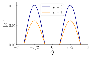
Figure 9: The squared modulus of the chiral order parameter $\kappa$ in Eq.(92) is plotted as a function of $Q$, at fixed $\Delta_{0}=0.6w$ (anisotropy parameter), for two values of $\mu$ (magnetic field). The maximum of chiral order occurs at $Q=\pm\pi/2$, its maximal value depends on $\mu$ and the onset of the chiral phase ($\kappa\neq 0$) is determined by the range $Q^{*}<|Q|<\pi-Q^{*}$, and only depends on the anisotropy parameter $\Delta_{0}$ [see Eq.(71)] and not on $\mu$.

As far as non-local spin correlations at arbitrary distance $l$ are concerned, their evaluation through fermionic correlation requires to account for the string operators appearing in the inverse Jordan-Wigner transformation (87)

$$\langle\sigma^{+}_{j}\sigma^{+}_{j+l}\rangle = e^{-iQ(2j+l)}\langle c^{\dagger}_{j}\prod^{l-1}_{n=j}\left(1-2c^{\dagger}_{n}c_{n}\right)c^{\dagger}_{j+l}\rangle$$ (93)

$$\langle\sigma^{-}_{j}\sigma^{-}_{j+l}\rangle = e^{iQ(2j+l)}\langle c_{j}\prod^{l-.1}_{n=j}\left(1-2c^{\dagger}_{n}c_{n}\right)c_{j+l}\rangle$$ (94)

$$\langle\sigma^{+}_{j}\sigma^{-}_{j+l}\rangle = e^{-iQl}\langle c^{\dagger}_{j}\prod^{l-1}_{n=j}\left(1-2c^{\dagger}_{n}c_{n}\right)c_{j+l}\rangle$$ (95)

$$\langle\sigma^{-}_{j}\sigma^{+}_{j+l}\rangle = e^{iQl}\langle c_{j}\prod^{l-1}_{n=j}\left(1-2c^{\dagger}_{n}c_{n}\right)c_{j+l}\rangle.$$ (96)

The right hand side of Eqs.(93)-(96) can be computed by applying Wick’s theorem and expressing spin correlations at a given distance $l$ as combination of products of the fermionic two-point correlation functions $\mathcal{C}(m)$ and $\mathcal{A}(m)$ determined in the previous section, for various $m$.

VII Summary and Conclusions

In this article we have investigated the correlation functions of the 1D Kitaev model in the presence of a spatially modulated phase of its superconducting order parameter, whose wavevector $Q$ identifies the finite net momentum $-2Q$ of the Cooper pairs. The model describes a $p$-wave topological superconductor crossed by an electrical current, and is characterized by two types of topological transitions. While in the regime $\Delta_{0}>w$ the ground state purely consists of Cooper pairs, and only a band topology transition between topologically trivial and non-trivial gapped phases can occur [see Fig.1(a)], in the regime $\Delta_{0}<w$ a gapless superconducting phase also appears in the $(Q,\mu)$ phase diagram [green region in Fig.1(b) and (c)] and the Fermi surface Lifshitz transition is additionally possible. We have found that such a rich scenario leads to various interesting effects in the correlation functions.

First, we have shown that for vanishing chemical potential, $\mu=0$, or for phase modulation wavevector equal to $Q=\pm\pi/2$, the correlations $\mathcal{C}(l)$ and $\mathcal{A}(l)$ at site distance $l$ exhibit an even/odd effect (see Fig.2). In particular, while the anomalous correlation $\mathcal{A}(l)$ is always strictly vanishing at any even $l$, the even/odd effect for the normal correlation function $\mathcal{C}$ in the case $Q=\pm\pi/2$ also depends on whether the system is in the gapped or gapless phase [see Tables 1 and  2].

Then, we have shown that the difference between the band topology and the Lifshitz transitions can be signalled by analyzing the behavior of the correlation functions $\mathcal{C}(l)$ and $\mathcal{A}(l)$ at short distance ($l=1,2$) as a function of the modulation wavevector $Q$. Our results for $l=1$ (see Figs.3, 4 and 5) highlight that across the band topology transition the anomalous correlation function $\mathcal{A}(1)$ behaves very smoothly in $Q$ and is not very informative about the transition, while the normal correlation function $\mathcal{C}(1)$ signals the transition only through a divergence of its derivative (upper right panels of Fig.4). This is a consequence of the direct closing of the gap at $k=0$ or $k=\pi$ across the two topologically distinct gapped phases and the related divergence of the correlation length from both sides of the transition, in agreement with the universality of the correlation length scaling discussed in Ref.[8]. In contrast, across the Lifshitz transition both correlations functions $\mathcal{C}(1)$ and $\mathcal{A}(1)$ exhibit sharp cusps, which reflect discontinuity jumps in their derivative (right panels of Fig.5). We have shown that a jump is the hallmark of the indirect closing of the gap at the Lifshitz transition and the appearance of unpaired fermions in the ground state. Such a difference between the two types of transitions is found also the correlation functions at distance $l=2$ (see Fig.6, 7 and 8). Indeed, despite the qualitatively different behavior with respect to the $l=1$ case, which can be appreciated by comparing Figs.3 and Fig.6, sharp cusps in both $|\mathcal{C}(2)|^{2}$ and $|\mathcal{A}(2)|^{2}$ are clearly found as a function of $Q$ across the Lifshitz transition (see Fig.8).

Furthermore, we have been able to determine the asymptotic behavior of $\mathcal{C}(l)$ and $\mathcal{A}(l)$ for long distance $l\gg 1$. In particular, in the gapped phase we have found that, depending on the parameter range, the exponential decay of correlation functions can actually acquire three different forms, identified by the symbols “$\circ$”, “$\cdot$” and “$-$” in the cyan and grey regions of Fig.1, and encoded in the pairs of equations (35)-(36), (59)-(60), and (67)-(68), respectively. Inside the gapless phase (green regions in Fig.1), correlations decay algebraically as given by Eqs.(V.0.2)-(V.0.2). Notably, for $\Delta_{0}>w$ both trivial and topological gapped phases are characterized only by the “$\circ$” type of exponential decay. In contrast, for $\Delta_{0}<w$, also the regions denoted by “$\cdot$” and “$-$” emerge. In particular, we have shown that the elliptic “$-$” region can be interpreted as that sub-portion of the gapped topological region of the parameter space that, by a sufficiently large increase of $Q$, allows the system to enter the gapless superconducting state.

Finally, we have shown that the Kitaev model with superconducting phase modulation can be mapped in a XY spin model, where $Q$ controls both the exchange coupling constants (84) and the strength (85) of a Dzyaloshinskii-Moriya interaction. We have shown that the gapless superconducting phase of the Kitaev model, where unpaired fermions appear in the ground states, can be interpreted as the spin chiral phase of the XY model, whose order parameter reaches its maximal values around for $Q=\pm\pi/2$ (see Fig.9). We have therefore used our results about fermionic correlations to evaluate also spin correlations between neighboring sites.

Implementations. Before concluding, we would like to briefly discuss some possible setups where the results obtained in this work could be applied. At the moment, there are mainly two promising setups for the realization of topological superconductivity. The first one is semiconductor nanowires with strong spin-orbit coupling, such as InSb and InAs, proximized by a superconducting layer (e.g., Al or Nb) and exposed to a longitudinal magnetic field [36, 37, 38, 39, 40, 41]. The second one is ferromagnetic atom chains deposited on a superconducting film [42, 43, 44]. Scanning tunneling microscopy has been proposed as a technique to measure local correlation functions in magnetic atom chains [27, 28], while spatial correlations in nanowires have been probed by X-ray scattering [74, 75]. Transport measurements are also closely related to correlation functions. Indeed the current $I=2\text{e}w\,\text{Im}\,\langle c^{\dagger}_{j}c_{j+1}\rangle/\hbar$ can be expressed in terms of the normal correlation function $\mathcal{C}(1)$ as

$$I=\frac{2\text{e}w}{\hbar}\left(\cos(Q)\mathcal{C}_{u}(1)-\sin(Q)\mathcal{C}_{p}(1)\right)\quad.$$ (97)

In particular, we would like to outline a connection between our results and the recent prediction that the electrical current through a topological superconductor exhibits cusps as a function of $Q$ [55]. On the one hand, the cusps in the current can now be interpreted as a straightforward consequence of the correlation singularity across the Lifshitz transition. On the other hand, because our findings show that such cusps are a general hallmark of such type of transition, their signature is expected to be observable in other correlation functions as well, like the anomalous correlation $\mathcal{A}$. The latter can be extracted from Andreev reflection spectroscopy [76, 77] and non-local correlations are accessible via crossed Andreev reflection and cross correlation measurements [78, 79, 80, 81].

Moreover, because our findings can also be interpreted in terms of spin chain models, we mention that nuclear magnetic resonance techniques enable one to determine correlation functions in magnetic systems even in out of equilibrium conditions [82]. Finally, spin models with adjustable spin-spin interactions can also be implemented with ions confined in a linear Paul trap, which can be manipulated using lasers. This approach allows both collective and individual control over ion spins through laser interactions, and enables one to access single-shot measurements of spin correlations [83, 84].

Appendix A Derivation of the real space correlations functions

In this Appendix we provide some details about the evaluation of the correlation functions (21) and (22) given in the Main Text. By re-expressing the real space operators through their Fourier modes, $c_{j}=N_{s}^{-1/2}\sum_{k\in{\rm BZ}}e^{ikj}c_{k}$, one can rewrite Eqs.(21) and (22) as

$$\mathcal{C}(j_{2}-j_{1}) = e^{iQ(j_{2}-j_{1})}\langle c^{\dagger}_{j_{1}}c_{j_{2}}\rangle=$$ (98)

$$= \frac{e^{iQ(j_{2}-j_{1})}}{N_{s}}\sum_{k_{1},k_{2}}e^{-ik_{1}j_{1}}e^{ik_{2}j_{2}}\langle c^{\dagger}_{k_{1}}c_{k_{2}}\rangle=$$

$$= \frac{1}{N_{s}}\sum_{k,k^{\prime}}e^{-i\left(kj_{1}-k^{\prime}j_{2}\right)}\langle c^{\dagger}_{k-Q}c_{k^{\prime}-Q}\rangle,$$

and

$$\mathcal{A}(j_{2}-j_{1}) = e^{-iQ(j_{2}+j_{1})}\langle c^{\dagger}_{j_{1}}c^{\dagger}_{j_{2}}\rangle$$ (99)

$$= e^{-iQ(j_{2}+j_{1})}\frac{1}{N_{s}}\sum_{k_{1},k_{2}}e^{-ik_{1}j_{1}}e^{-ik_{2}j_{2}}\langle c^{\dagger}_{k_{1}}c^{\dagger}_{k_{2}}\rangle=$$

$$= \frac{1}{N_{s}}\sum_{k,k^{\prime}}e^{-i\left(kj_{1}-k^{\prime}j_{2}\right)}\langle c^{\dagger}_{k-Q}c^{\dagger}_{-k^{\prime}-Q}\rangle,$$

respectively. The correlations $\langle c^{\dagger}_{k-Q}c_{k^{\prime}-Q}\rangle$, and $\langle c^{\dagger}_{k-Q}c^{\dagger}_{-k^{\prime}-Q}\rangle$ appearing in Eqs.(98)-(99) can now be computed by inverting Eqs.(11) in favor of the $c_{k-Q},c^{\dagger}_{k-Q}$ operators

$$\left\{\begin{array}[]{lcl}c_{k-Q}&=&u_{Q}(k)\gamma_{k-Q}-v^{*}_{Q}(k)\,\gamma^{\dagger}_{-k-Q}\\ c^{\dagger}_{k-Q}&=&u_{Q}(k)\gamma^{\dagger}_{k-Q}-v_{Q}(k)\gamma_{-k-Q}\end{array}\right.$$ (100)

and by exploiting the action of the $\gamma$-Bogolubov quasi-particles onto the current carrying ground state $|G(Q)\rangle$ given in Eq.(12). Such an action depends on the specific Brillouin sector $S_{p}$, $S_{e}$ or $S_{h}$ where the $k$-wavevector is located, namely $\gamma_{k-Q}\ket{G(Q)}=0$ for $k\in S_{+}\equiv S_{p}\cup S_{h}$ and $\gamma^{\dagger}_{k-Q}\ket{G(Q)}=0$ for $k\in S_{-}\equiv S_{e}$. Therefore, one has to consider the following cases
1.  $k,k^{\prime}\in S_{p}$

$$\begin{array}[]{ccl}\langle\gamma^{\dagger}_{k-Q}\gamma_{k^{\prime}-Q}\rangle&=&\langle\gamma^{\dagger}_{k-Q}\gamma^{\dagger}_{-k^{\prime}-Q}\rangle=\\ &=&\langle\gamma_{-k-Q}\gamma_{k^{\prime}-Q}\rangle=0\\ \langle\gamma_{-k-Q}\gamma^{\dagger}_{-k^{\prime}-Q}\rangle&=&\delta_{k,k^{\prime}}\end{array}$$ (101)

2. $k\in S_{h},\,-k\in S_{e}$

$$\begin{array}[]{l}\langle\gamma^{\dagger}_{k-Q}\gamma_{k^{\prime}-Q}\rangle=\langle\gamma^{\dagger}_{k-Q}\gamma^{\dagger}_{-k^{\prime}-Q}\rangle=\\ =\langle\gamma_{-k-Q}\gamma_{k^{\prime}-Q}\rangle=\langle\gamma_{-k-Q}\gamma^{\dagger}_{-k^{\prime}-Q}\rangle=0\end{array}$$ (102)

3. $k\in S_{e},\,-k\in S_{h}$

$$\begin{array}[]{ccl}\langle\gamma^{\dagger}_{k-Q}\gamma_{k^{\prime}-Q}\rangle&=&\langle\gamma_{-k-Q}\gamma^{\dagger}_{-k^{\prime}-Q}\rangle=\delta_{k,k^{\prime}}\\ \langle\gamma^{\dagger}_{k-Q}\gamma^{\dagger}_{-k^{\prime}-Q}\rangle&=&\langle\gamma_{-k-Q}\gamma_{k^{\prime}-Q}\rangle=0\\ \end{array}$$ (103)

Exploiting the above results one obtains the correlations in momentum space

$$\langle c^{\dagger}_{k-Q}c_{k^{\prime}-Q}\rangle=\left\{\begin{array}[]{ccc}\left|v_{Q}(k)\right|^{2}\delta_{k,k^{\prime}}&&k\in S_{p}\\ 0&&k\in S_{h}\\ \delta_{k,k^{\prime}}&&k\in S_{e}\end{array}\right.,$$ (104)

$$\langle c_{-k-Q}c^{\dagger}_{-k^{\prime}-Q}\rangle=\left\{\begin{array}[]{ccc}\left|u_{Q}(k)\right|^{2}\delta_{k,k^{\prime}}&&k\in S_{p}\\ 0&&k\in S_{h}\\ \delta_{k,k^{\prime}}&&k\in S_{e}\end{array}\right.,$$ (105)

$$\langle c_{-k-Q}c_{k^{\prime}-Q}\rangle=\left\{\begin{array}[]{ccc}-u_{Q}(k)v^{*}_{Q}(k)\delta_{k,k^{\prime}}&&k\in S_{p}\\ 0&&k\in S_{h}\\ 0&&k\in S_{e}\end{array}\right.,$$ (106)

$$\langle c^{\dagger}_{k-Q}c^{\dagger}_{-k^{\prime}-Q}\rangle=\left\{\begin{array}[]{ccc}-u_{Q}(k)v_{Q}(k)\delta_{k,k^{\prime}}&&k\in S_{p}\\ 0&&k\in S_{h}\\ 0&&k\in S_{e}\end{array}\right.,$$ (107)

where $u_{Q}(k)$ and $v_{Q}(k)$ are given by Eq.(9). Replacing Eqs.(104)-(105)-(106)-(107) in Eq.(98) and Eq.(99), and denoting $l=j_{2}-j_{1}$, it is straightforward to obtain

$$\mathcal{C}(l) = \frac{1}{N_{s}}\left(\sum_{k\in S_{p}}e^{ikl}\left|v_{Q}(k)\right|^{2}+\sum_{k\in S_{e}}e^{ikl}\right)$$ (108)

$$\mathcal{A}(l) = -\frac{1}{N_{s}}\sum_{k\in S_{p}}e^{ikl}u_{Q}(k)v_{Q}(k)$$ (109)

Substituting Eq.(9) into Eq.(109), and taking the thermodynamic limit $N_{s}\rightarrow\infty$, one obtains Eq.(26) of the Main Text. Moreover, exploiting the mirror symmetries $S_{e}\rightarrow S_{h}$ and $S_{p}\rightarrow S_{p}$ under $k\rightarrow-k$, one can rewrite Eq.(108) as

$$\mathcal{C}(l)=$$

$$= \frac{1}{2N_{s}}\left(\sum_{k\in{\rm BZ}}\cos(kl)-\sum_{k\in S_{p}}\frac{\xi(k;Q)}{h(k;Q)}+2\sum_{k\in S_{e}}\sin(kl)\right)$$

whence Eq.(24) and (25) of the Main Text are obtained by recalling that $l\neq 0$ is assumed, and by taking the thermodynamic limit $N_{s}\rightarrow\infty$.

Appendix B Details about correlation functions in the cases $\mu=0$ and $Q=\pm\pi/2$

In this Appendix we prove the even/odd effect occurring for $\mu=0$ or $Q=\pm\pi/2$ and discussed in Sec.III. Moreover, we provide the analytical expressions of the correlation functions at some values of $l$. For definiteness, we shall provide the proof for the normal correlation function $\mathcal{C}(l)$ in the case $\mu=0$, as the proof for the anomalous correlation $\mathcal{A}$ or for $Q=\pm\pi/2$ follows along the same lines. We start by analyzing the unpaired fermion contribution $\mathcal{C}_{u}(l)$, which vanishes in the gapped phase, $\mathcal{C}_{u}(l)\equiv 0$, while in the gapless phase is exactly given by Eq.(27). We now note that, for $\mu=0$, the two wavevectors in Eq.(20) share the same magnitude, which we can denote as

$$k^{*}_{Q}=|k^{*}_{\pm}(\mu=0)|=\arcsin\left(\frac{|\cos{Q}|}{\sqrt{1-\frac{\Delta_{0}^{2}}{w^{2}}}}\right)\quad.$$ (111)

Thus, from Eq.(27) one obtains

$$\left.\mathcal{C}_{u}(l)\right|_{\mu=0}=-\frac{\text{sgn}(Q)}{2\pi}\frac{1}{l}\left(1-(-1)^{l}\right)\cos(k^{*}_{Q}l)\quad,$$ (112)

whence we deduce that $\mathcal{C}_{u}(l)$ vanishes for even values of $l$. Turning now to the pair contribution $\mathcal{C}_{p}$, we observe that in its general expression Eq.(24) both the integrand function and the integration domain $S_{p}$ are symmetric under $k\rightarrow-k$, implying that this expression can be rewritten as an integral over the positive-$k$ values of $S_{p}$ only. Focussing first on the gapless phase, where the $S_{p}$ domain is given by Eq.(19), one can rewrite Eq.(24) as

$$\left.\mathcal{C}_{p}(l)\right|_{\mu=0} = -\frac{\cos{Q}}{2\pi}\left\{\int_{0}^{k^{*}_{Q}}\frac{\cos k\,\cos(kl)\,dk\,}{\sqrt{\cos^{2}k\cos^{2}{Q}+\frac{\Delta_{0}^{2}}{w^{2}}\sin^{2}k}}\,+\,\right.$$

$$\left.\hskip 14.22636pt+\int_{\pi-k^{*}_{Q}}^{\pi}\frac{\cos k\,\cos(kl)\,dk\,}{\sqrt{\cos^{2}k\cos^{2}{Q}+\frac{\Delta_{0}^{2}}{w^{2}}\sin^{2}k}}\right\}\,\,.$$

Changing $k\rightarrow\pi-k$ in the second integral, and exploiting $\cos(\pi l-kl)=(-1)^{l}\cos(kl)$, one finds

$$\left.\mathcal{C}_{p}(l)\right|_{\mu=0}=-\frac{1-(-1)^{l}}{2}\,\mathcal{Q}^{n}_{p}(l;k^{*}_{Q})\quad,$$ (113)

whence we realize that such expression vanishes for $l$ even. Here we have introduced

$$\begin{array}[]{lcl}\mathcal{Q}^{n}_{p}(l;\alpha)&\doteq&\displaystyle\frac{\cos{Q}}{\pi}\int_{0}^{\alpha}\frac{\cos k\,\cos(kl)\,dk\,}{\sqrt{\cos^{2}k\cos^{2}{Q}+\frac{\Delta_{0}^{2}}{w^{2}}\sin^{2}k}}=\\ &&\\ &=&\displaystyle\frac{\mbox{sgn}(\cos{Q})}{\pi}\int_{0}^{\alpha}dk\,\frac{\cos k\,\cos(kl)}{\sqrt{\cos^{2}k+\delta_{Q}\sin^{2}k}}\end{array}$$ (114)

with

$$\delta_{Q}=\frac{\Delta_{0}^{2}}{w^{2}\cos^{2}{Q}}\quad.$$ (115)

The result for the gapped phase is obtained by replacing $k^{*}_{Q}\rightarrow\pi/2$.

For the case $Q=\pm\pi/2$, following similar arguments and denoting

$$k^{*}_{\mu}=|k^{*}_{+}(Q=\pm\frac{\pi}{2}|=\arcsin\left(\frac{|\mu|}{2\sqrt{w^{2}-\Delta_{0}^{2}}}\right)\quad,$$ (116)

one finds for the gapless phase

$$\left.\mathcal{C}_{p}(l)\right|_{Q=\pm\frac{\pi}{2}}=\frac{1+(-1)^{l}}{2}\,\mathcal{R}^{n}_{p}(l;k^{*}_{\mu})\quad,$$ (117)

where we have introduced

$$\mathcal{R}^{n}(l;\alpha) \doteq \displaystyle\frac{\mu}{\pi}\int_{0}^{\alpha}dk\,\frac{\cos(kl)}{\sqrt{\mu^{2}+4\Delta_{0}^{2}\sin^{2}k}}=$$ (118)

$$= \frac{\mbox{sgn}(\mu)}{\pi}\int_{0}^{\alpha}dk\,\frac{\cos(kl)}{\sqrt{1+4\delta_{\mu}\sin^{2}k}}$$

with

$$\delta_{\mu}=\frac{\Delta_{0}^{2}}{\mu^{2}}\quad.$$ (119)

For the gapped phase the same formula (117) holds, with $k^{*}_{\mu}\rightarrow\pi/2$. In both cases, Eq.(117) implies that $\mathcal{C}_{p}$ vanishes for $l$ odd.

We conclude this Appendix by mentioning that, at $\mu=0$ or $Q=\pm\pi/2$ and for small values of $l$, it is also possible to find from Eq.(114) and (118) an exact analytical expression of the correlation functions in terms of incomplete elliptic functions of the first and second kind, $F$ and $E$. Here we limit ourselves to provide the (non vanishing) expressions for $l=1,2$ in the gapless phase.

For the case $\mu=0$ one has

$$\mathcal{C}_{p}(1)=\frac{\text{sgn}(\cos{Q})}{\pi}\left(\frac{\delta_{Q}F(k^{*}_{Q};1-\delta_{Q})-E(k^{*}_{Q};1-\delta_{Q})}{1-\delta_{Q}}\right)$$ (120)

and

$$\mathcal{A}(1)=\frac{\sqrt{\delta_{Q}}}{\pi}\left(\frac{E(k^{*}_{Q};1-\delta_{Q})-F(k^{*}_{Q};1-\delta_{Q})}{1-\delta_{Q}}\right)$$ (121)

while for the case $Q=\pm\pi/2$ one obtains

$$\mathcal{C}_{p}(2)=\frac{\text{sgn}(\mu)}{\pi}\left(\frac{(1+2\delta_{\mu})F(k^{*}_{\mu};-4\delta_{\mu})}{2\delta_{\mu}}-\frac{E(k^{*}_{\mu};-4\delta_{\mu})}{2\delta_{\mu}}\right)$$

and

$$\mathcal{A}(1)=\frac{\sqrt{\delta_{\mu}}}{\pi}\left(\frac{F(k^{*}_{\mu};-4\delta_{\mu})-E(k^{*}_{\mu};-4\delta_{\mu})}{2\delta_{\mu}}\right)$$ (123)

For the gapped phase, the corresponding results are obtained from the above formulas by replacing $k^{*}_{Q}\rightarrow\pi/2$ and $k^{*}_{\mu}\rightarrow\pi/2$, thereby obtaining expressions in terms of the complete elliptic integrals $K$ and $E$.

Appendix C Asymptotic Expansion of the correlations functions in the gapped phase

In this Appendix we provide details of the derivation of results about the asymptotic behavior of the correlation functions at long distance ($l\gg 1$) given in Section V.0.1. The functions appearing in Eqs.(33) and (34) exhibit four branch points at $z=Z_{j}$ given by

$$\begin{array}[]{l}Z_{1,2}=\displaystyle\frac{\frac{\mu}{2}\,\mbox{sgn}(\cos{Q})\pm\sqrt{\Delta_{0}^{2}+\frac{\mu^{2}}{4}-w^{2}\cos^{2}{Q}}}{w|\cos{Q}|+\Delta_{0}}\\ \\ Z_{3,4}=\displaystyle\frac{\frac{\mu}{2}\,\mbox{sgn}(\cos{Q})\pm\sqrt{\Delta_{0}^{2}+\frac{\mu^{2}}{4}-w^{2}\cos^{2}{Q}}}{w|\cos{Q}|-\Delta_{0}}\end{array}\quad,$$ (124)

whose location depends on the paramters $\Delta_{0}$, $\mu$ and $Q$. Note that the case $|\mu|=2w|\cos{Q}|$ is ruled out from the gapped phase parameter conditions (16), since in such a case two of the branch points (124) coalesce into a pole on the circle at either $z=+1$ or $z=-1$. This corresponds to the direct closing of the superconducting gap at $k=0$ or $k=\pi$, and identifies the separatrix between the two topologically distinct gapped phases, as observed above. Avoiding this singularity and focussing on the gapped phases, two branch points, which we shall denote as $z^{**}_{\pm}$, lie outside the unit circle ($|z^{**}_{\pm}|>1$), whereas, as observed in the Main Text, the two inner branch points ($|z^{*}_{\pm}|<1$) can have three different configurations in the complex plane, namely (1) both real and with opposite sign; (2) both real and with equal signs; (3) complex conjugate pair. These are illustrated in Fig.10, and determine the three different types of asymptotic behavior in the gapped phase. By applying Cauchy theorem to Eqs.(33) and (34), one can rewrite

$$\mathcal{C}_{p}(l) = +\frac{1}{4\pi}{\rm Im}\left\{\oint_{b.cut}dz\frac{z^{l-1}\,g(z)}{\mathcal{D}(z)}\right\}$$ (125)

$$\mathcal{A}(l) = -\frac{1}{4\pi}{\rm Im}\left\{\oint_{b.cut}dz\frac{z^{l-1}\,\,f(z)}{\mathcal{D}(z)}\right\}$$ (126)

where $\mathcal{D}(z)=\sqrt{g^{2}(z)-f^{2}(z)}$, and ”b.cut” denotes the inner branch cuts, taken clockwise, as also shown in Fig.10. Here we have exploited the fact that the integrals along infinitesimally small circles around the branch cuts vanish. One can now determine the values of the denominator $\mathcal{D}(z)$ appearing in Eqs.(125)-(126) along the branch cuts, analyzing the three possible configurations of the branch points $z^{*}_{\pm}$.

(1): $z^{*}_{\pm}$ real with opposite sign
This configuration occurs when the conditions (38) are fulfilled. In this case, the outer branch points are given by $z^{**}_{+}=1/z^{*}_{+}>0$ and $z^{**}_{-}=1/z^{*}_{-}<0$. The values of $\mathcal{D}(z)$ along the inner branch cut in Fig.10(1) are

$$\left\{\begin{array}[]{lcl}\mathcal{D}(x\pm i\epsilon)=\pm iD_{1}(x)&&x>0\\ \mathcal{D}(x\pm i\epsilon)=\mp iD_{1}(x)&&x<0\end{array}\right.$$ (127)

where

$$D_{1}(x)=\sqrt{\frac{\Delta_{0}^{2}-w^{2}\cos^{2}{Q}}{x^{2}}}\times$$

$$\times\sqrt{(z^{*}_{+}-x)\,(x-z^{*}_{-})\,(z^{**}_{+}-x)\,\,(x-z^{**}_{-})}$$

Inserting Eqs.(127)-(C) into Eq.(125) one obtains

$$\mathcal{C}_{p}(l) = \displaystyle-\frac{1}{2\pi}\,\frac{1}{\sqrt{\frac{\Delta_{0}^{2}}{w^{2}}-\cos^{2}{Q}}}\,\left\{\int_{0}^{z_{+}^{*}}\,dx\frac{x^{(l-1)}}{\sqrt{z^{*}_{+}-x}}f^{n,+}_{reg}(x)-(-1)^{l}\int_{0}^{|z_{-}^{*}|}\,dx\frac{x^{(l-1)}}{\sqrt{|z^{*}_{-}|-x}}f^{n,-}_{reg}(x)\right\}$$ (129)

where

$$f^{n,+}_{reg}(x) = \frac{(1+x^{2})\cos{{Q}}-\frac{\mu}{w}x}{\sqrt{\,\,(|z^{*}_{-}|+x)\,(\frac{1}{z^{*}_{+}}-x)\,\,(\frac{1}{|z^{*}_{-}|}+x)}}$$ (130)

$$f^{n,-}_{reg}(x) = \frac{(1+x^{2})\cos{{Q}}+\frac{\mu}{w}x}{\sqrt{\,(z^{*}_{+}+x)\,\,(\frac{1}{z^{*}_{+}}+x)\,\,(\frac{1}{|z^{*}_{-}|}-x)}}$$ (131)

In the first integral the term $x^{l-1}$ ranges from 0 to $(z^{*}_{+})^{l-1}$, which is exponentially small for $l\rightarrow\infty$ and strongly suppresses the contribution from $f^{n,+}_{reg}(x)$ away from $x\simeq z^{*}_{+}$. Similarly, in the second integral, the contribution from $f^{n,-}_{reg}(x)$ away from $x\simeq|z^{*}_{-}|$ is negligible. Therefore, in the $l\gg 1$ limit one can approximate Eq. (129) as

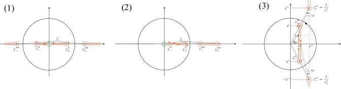
Figure 10: The three different configurations of the inner branch points $z^{*}_{\pm}$ of the denominator $\mathcal{D}(z)=\sqrt{g^{2}(z)-f^{2}(z)}$ appearing in Eqs.(125)-(126). The branch cuts are highlighted in red.

$$\mathcal{C}_{p}(l) \sim \displaystyle-\frac{1}{2\pi}\,\frac{1}{\sqrt{\frac{\Delta_{0}^{2}}{w^{2}}-\cos^{2}{Q}}}\,\left\{f^{n,+}_{reg}(z^{*}_{+})\int_{0}^{z_{+}^{*}}\frac{x^{(l-1)}}{\sqrt{z^{*}_{+}-x}}\,dx\,-(-1)^{l}f^{n,-}_{reg}(|z^{*}_{-}|)\int_{0}^{|z_{-}^{*}|}\frac{x^{(l-1)}}{\sqrt{|z^{*}_{-}|-x}}\,dx\right\}$$ (132)

A similar expression can be obtained for $\mathcal{A}(l)$ inserting Eq.(127) into Eq.(126). Using the identity

$$\int_{0}^{a}\frac{x^{(l-1)}}{\sqrt{a-x}}\,dx=a^{l-\frac{1}{2}}\,\sqrt{\pi}\frac{\Gamma(l)}{\Gamma\left(l+\frac{1}{2}\right)}\simeq\sqrt{\frac{\pi}{a\,l}}\,a^{l}\,$$ (133)

where we have exploited $\Gamma(l+\frac{1}{2})\sim\Gamma(l)\,l^{1/2}$ for $l\rightarrow\infty$, one obtains Eqs.(35) and (36), where

$$\alpha^{\pm}_{1}= \frac{wA^{\pm}_{1}}{\sqrt{\pi}\sqrt{\Delta^{2}_{0}-w^{2}\cos^{2}\left(Q\right)}},$$ (134)

$$\beta^{\pm}_{1}= \frac{\Delta_{0}B^{\pm}_{1}}{\sqrt{\pi}\sqrt{\Delta^{2}_{0}-w^{2}\cos^{2}\left(Q\right)}}$$ (135)

with

$$A^{\pm}_{1}= \frac{\left(1-\left|z^{*}_{\pm}\right|^{2}\right)\cos\left(Q\right)\mp\frac{\mu}{w}\left|z^{*}_{\pm}\right|}{\sqrt{\left|z^{*}_{\pm}\right|\left(\left|z^{*}_{+}\right|+\left|z^{*}_{-}\right|\right)\left(\frac{1}{\left|z^{*}_{\mp}\right|}+\left|z^{*}_{\pm}\right|\right)\left(\frac{1}{\left|z^{*}_{\pm}\right|}-\left|z^{*}_{\pm}\right|\right)}}$$ (136)

$$B^{\pm}_{1}= \frac{1-\left|z^{*}_{\pm}\right|^{2}}{\sqrt{\left|z^{*}_{\pm}\right|\left(\left|z^{*}_{+}\right|+\left|z^{*}_{-}\right|\right)\left(\frac{1}{\left|z^{*}_{\mp}\right|}+\left|z^{*}_{\pm}\right|\right)\left(\frac{1}{\left|z^{*}_{\pm}\right|}-\left|z^{*}_{\pm}\right|\right)}}.$$ (137)

(2): $z^{*}_{\pm}$ real roots with the same sign
This configuration occurs when the parameters fulfill Eqs.(63). In this case one has $z^{**}_{+}=1/z^{*}_{-}$ and $z^{**}_{-}=1/z^{*}_{+}$. The values of $\mathcal{D}(z)$ along the inner branch cut in Fig.10(2) are

$$\mathcal{D}(x\pm i\epsilon)=\pm i\,\sigma^{*}\,D_{2}(x)$$ (138)

where $\sigma^{*}$ is given by Eq.(58), and

$$D_{2}(x)=\sqrt{\frac{w^{2}\cos^{2}{Q}-\Delta_{0}^{2}}{{x^{*}}^{2}+y^{2}}}\times$$ (139)

$$\times\sqrt{(z^{*}_{+}-x)\,(x-z^{*}_{-})\,(z^{**}_{+}-x)\,\,(z^{**}_{-}-x)}\quad.$$

Inserting Eqs.(138)-(139) into Eq.(125), and denoting

$$\begin{array}[]{lcl}x_{M}&=&\mbox{max}(|z^{*}_{+}|,|z^{*}_{-}|)\\ x_{m}&=&\mbox{min}(|z^{*}_{+}|,|z^{*}_{-}|)\end{array}$$ (140)

one obtains

$$\mathcal{C}_{p}(l)=\displaystyle\frac{1}{2\pi}\frac{{\sigma^{*}}^{l-1}}{\sqrt{\cos^{2}{Q}-\frac{\Delta_{0}^{2}}{w^{2}}}}\,\times$$

$$\int_{x_{m}}^{x_{M}}\!\!\!dx\frac{x^{l-1}\,\left((1+x^{2})\cos{{Q}}-\frac{\mu}{w}x\,\sigma^{*}\right)}{\sqrt{\,(x_{M}-x)\,(x-x_{m})\,(\frac{1}{x_{M}}-x)\,(\frac{1}{x_{m}}-x)}}$$

A similar expression is obtained for $\mathcal{A}(l)$. Applying the same approximation strategy as in the case (1) for $l\gg 1$, one obtains Eqs.(59) and (60), where

$$\alpha_{M} = \frac{1}{\sqrt{\cos^{2}{Q}-\frac{\Delta_{0}^{2}}{w^{2}}}}\,\frac{(1+x_{M}^{2})\cos{{Q}}-\frac{\mu}{w}x_{M}\sigma^{*}}{\sqrt{\pi\,(x_{M}-x_{m})\,(\frac{1}{x_{m}}-x_{M})\,(1-x_{M}^{2})\,}}$$

$$\alpha_{m} = \frac{1}{\sqrt{\cos^{2}{Q}-\frac{\Delta_{0}^{2}}{w^{2}}}}\,\frac{(1+x_{m}^{2})\cos{{Q}}-\frac{\mu}{w}x_{m}\sigma^{*}}{\sqrt{\pi\,(x_{M}-x_{m})\,(\frac{1}{x_{M}}-x_{m})\,(1-x_{m}^{2})\,}}$$

$$\beta_{M} = \frac{\frac{\Delta_{0}}{w}}{\sqrt{\cos^{2}{Q}-\frac{\Delta_{0}^{2}}{w^{2}}}}\,\sqrt{\frac{1-x_{M}^{2}}{\pi\,(x_{M}-x_{m})\,(\frac{1}{x_{m}}-x_{M})}}$$

$$\beta_{m} = \frac{\frac{\Delta_{0}}{w}}{\sqrt{\cos^{2}{Q}-\frac{\Delta_{0}^{2}}{w^{2}}}}\,\sqrt{\frac{1-x_{m}^{2}}{\pi\,(x_{M}-x_{m})\,(\frac{1}{x_{M}}-x_{m})}}$$

(3): $z^{*}_{\pm}=x^{*}\pm iy^{*}$ a complex conjugate pair
This configuration occurs in the parameter range (64). In this case $z^{**}_{+}=1/z^{*}_{-}$ and $z^{**}_{-}=1/z^{*}_{+}$, as displayed in Fig.10(3). The real and imaginary parts of the inner roots are given in Eqs.(65)-(66) of the Main Text, while for the outer roots $z^{**}_{\pm}=x^{**}\pm iy^{**}$, one has

$$x^{**} = \displaystyle\frac{\frac{\mu}{2}\,\mbox{sgn}(\cos{{Q}})}{w|\cos{{Q}}|-\Delta_{0}}$$ (146)

$$y^{**} = \frac{\sqrt{w^{2}\cos^{2}{Q}-\Delta_{0}^{2}-\frac{\mu^{2}}{4}}}{w|\cos{{Q}}|-\Delta_{0}}\quad.$$ (147)

The values of $\mathcal{D}(z)$ along the branch cut are given by

$$\mathcal{D}(x^{*}\pm\epsilon+iy)=\pm\,D_{3}(y)e^{-i(\Delta\varphi(y)+\theta(y))}$$ (148)

where

$$D_{3}(y) = \sqrt{\frac{w^{2}\cos^{2}{Q}-\Delta_{0}^{2}}{{x^{*}}^{2}+y^{2}}}\times$$ (149)

$$\times\sqrt{\,\rho_{+}(y)\,\,\rho_{-}(y)\,\,r_{+}(y)\,\,r_{-}(y)}$$

with

$$\rho_{\pm}(y) = y^{*}\mp y\,$$ (150)

$$r_{\pm}(y) = \,\,\sqrt{(x^{*}-x^{**})^{2}+(y\mp y^{**})^{2}}\,$$ (151)

$$|z(y)| = \sqrt{{x^{*}}^{2}+y^{2}}$$ (152)

$$\theta(y) = \mbox{arg}(x^{*}+iy)\,\in[-\pi,\pi]$$ (153)

$$\Delta\varphi(y) = \frac{1}{2}\left\{\arctan\left(\frac{x^{**}-x^{*}}{y^{**}-y}\right)-\right.$$ (154)

$$\left.\hskip 28.45274pt\arctan\left(\frac{x^{**}-x^{*}}{y^{**}+y}\right)\right)$$

Inserting Eqs.(148)-(149) into Eq.(125) one obtains

$$\mathcal{C}_{p}(l) = \displaystyle\frac{1}{\pi}\frac{1}{\sqrt{\cos^{2}{Q}-\frac{\Delta_{0}^{2}}{w^{2}}}}\,\int_{0}^{y^{*}}\frac{|z(y)|^{l}}{\sqrt{({y^{*}}^{2}-y^{2})\,\,r_{+}(y)\,\,r_{-}(y)}}\,\,\times$$ (155)

$$\hskip 28.45274pt\displaystyle\times\left\{\sin\left[\Delta\varphi(y)+l\,\theta(y)\right]\,\cos{{Q}}\,(|z(y)|-|z(y)|^{-1})\sin{\theta(y)}-\right.$$

$$\displaystyle\hskip 34.14322pt\left.-\cos\left[\Delta\varphi(y)+l\,\theta(y)\right]\left(\cos{{Q}}\,(|z(y)|+|z(y)|^{-1})\cos{\theta(y)}-\frac{\mu}{w}\right)\right\}\,dy=$$

$$= \int_{0}^{y^{*}}\frac{({x^{*}}^{2}+y^{2})^{\frac{l-1}{2}}}{\sqrt{y^{*}-y}}\,\left\{F^{n}_{s}(y)\sin[l\theta(y)]+F^{n}_{c}(y)\cos[l\theta(y)]\right\}\,dy$$

where

$$F^{n}_{s}(y) = \frac{1}{\pi}\frac{1}{\sqrt{\cos^{2}{Q}-\frac{\Delta_{0}^{2}}{w^{2}}}}\,\frac{1}{\sqrt{(y^{*}+y)\,\,r_{+}(y)\,\,r_{-}(y)}}\times$$ (156)

$$\times\left\{\cos\left[\Delta\varphi(y)\right]\,\cos{{Q}}\,\,(|z(y)|^{2}-1)\sin{\theta(y)}+\sin\left[\Delta\varphi(y)\right]\left(\cos{{Q}}\,(|z(y)|^{2}+1)\cos{\theta(y)}-\frac{\mu}{w}\right)\right\}$$

$$F^{n}_{c}(y) = \frac{1}{\pi}\frac{1}{\sqrt{\cos^{2}{Q}-\frac{\Delta_{0}^{2}}{w^{2}}}}\,\frac{1}{\sqrt{(y^{*}+y)\,\,r_{+}(y)\,\,r_{-}(y)}}\times$$ (157)

$$\,\,\times\left\{\sin\left[\Delta\varphi(y)\right]\,\cos{{Q}}\,\,(|z(y)|^{2}-1)\sin{\theta(y)}-\cos\left[\Delta\varphi(y)\right]\left(\cos{{Q}}\,(|z(y)|^{2}+1)\cos{\theta(y)}-\frac{\mu}{w}\right)\right\}$$

A similar expression can be obtained for $\mathcal{A}(l)$. In the regime $|x^{*}|\ll y^{*}$, we observe that, for $l\gg 1$, the function $({x^{*}}^{2}+y^{2})^{\frac{l-1}{2}}$ suppresses exponentially in $l$ the contribution from $F^{n}_{c/s}(y)$ away from $y\simeq y^{*}$. Therefore, we can approximate Eq.(155) as

$$\mathcal{C}_{p}(l) \sim \left\{{F}^{n}_{s}(y^{*})\sin[l\theta^{*}]+{F}^{n}_{c}(y^{*})\cos[l\theta^{*}]\right\}\,\,\times$$ (158)

$$\,\times\int_{0}^{y^{*}}\frac{({x^{*}}^{2}+y^{2})^{\frac{l-1}{2}}}{\sqrt{y^{*}-y}}\,\,dy$$

where

$$\theta^{*}=\theta(y^{*})=\mbox{arg}(z^{*}_{+})\quad.$$ (159)

Moreover, again for $|x^{*}|\ll y^{*}$, the integral appearing in Eq.(158) can be fairly well approximated as

$$\int_{0}^{y^{*}}\frac{({x^{*}}^{2}+y^{2})^{\frac{l-1}{2}}}{\sqrt{y^{*}-y}}\,\,dy \sim ({x^{*}}^{2}+{y^{*}}^{2})^{\frac{l}{2}}\,\sqrt{\frac{\pi}{{y^{*}}\,l}}\,=$$ (160)

$$= |z^{*}_{+}|^{l}\,\sqrt{\frac{\pi}{{y^{*}}\,l}}$$

Inserting Eq.(160) into Eq.(158) and proceeding in a similar way for $\mathcal{A}(l)$, one obtains Eqs.(67) and (68), where

$$\alpha^{s}_{3} = \frac{1}{\sqrt{2\pi}}\frac{1}{\sqrt{\cos^{2}{Q}-\frac{\Delta_{0}^{2}}{w^{2}}}}\,\frac{1}{\sqrt{{y^{*}}^{2}\,\,r_{+}(y^{*})\,\,r_{-}(y^{*})}}\times\left\{\cos\left[\Delta\varphi(y^{*})\right]\,\cos{{Q}}\,\,(|z^{*}_{+}|^{2}-1)\sin{\theta^{*}}+\right.$$ (161)

$$\hskip 199.16928pt\left.+\sin\left[\Delta\varphi(y^{*})\right]\left(\cos{{Q}}\,(|z^{*}_{+}|^{2}+1)\cos{\theta^{*}}-\frac{\mu}{w}\right)\right\}$$

$$\alpha^{c}_{3} = \frac{1}{\sqrt{2\pi}}\frac{1}{\sqrt{\cos^{2}{Q}-\frac{\Delta_{0}^{2}}{w^{2}}}}\,\frac{1}{\sqrt{{y^{*}}^{2}\,\,r_{+}(y^{*})\,\,r_{-}(y^{*})}}\times\left\{\sin\left[\Delta\varphi(y^{*})\right]\,\cos{{Q}}\,\,(|z^{*}_{+}|^{2}-1)\sin{\theta^{*}}-\right.$$ (162)

$$\hskip 199.16928pt\left.-\cos\left[\Delta\varphi(y^{*})\right]\left(\cos{{Q}}\,\left(\left|z^{*}_{+}\right|^{2}+1\right)\cos{\theta^{*}}-\frac{\mu}{w}\right)\right\}$$

$$\beta^{s}_{3} = -\frac{1}{\sqrt{2\pi\,}}\frac{\frac{\Delta_{0}}{w}}{\sqrt{\cos^{2}{Q}-\frac{\Delta_{0}^{2}}{w^{2}}}}\frac{1}{\sqrt{{y^{*}}^{2}\,\,r_{+}(y^{*})\,\,r_{-}(y^{*})}}\times$$ (163)

$$\hskip 34.14322pt\times\left\{\cos\left[\Delta\varphi(y^{*})\right]\,(|z^{*}_{+}|^{2}+1)\,\sin{\theta^{*}}+\sin\left[\Delta\varphi(y^{*})\right]\,(|z^{*}_{+}|^{2}-1)\cos{\theta^{*}}\right\}$$

$$\beta^{c}_{3} = -\frac{1}{\sqrt{2\pi\,}}\frac{\frac{\Delta_{0}}{w}}{\sqrt{\cos^{2}{Q}-\frac{\Delta_{0}^{2}}{w^{2}}}}\frac{1}{\sqrt{{y^{*}}^{2}\,\,r_{+}(y^{*})\,\,r_{-}(y^{*})}}\times$$ (164)

$$\hskip 34.14322pt\times\left\{\sin\left[\Delta\varphi(y^{*})\right]\,\,\,(|z^{*}_{+}|^{2}+1)\sin{\theta^{*}}-\cos\left[\Delta\varphi(y^{*})\right]\,(|z^{*}_{+}|^{2}-1)\cos{\theta^{*}}\right\}$$

and $r_{\pm}(y)$ and $\Delta\varphi(y)$ are given in Eqs.(151) and (154), respectively.

Appendix D Asymptotic expansions of the correlation functions in the Gapless Phase

In this Appendix, we provide details about the derivation of the asymptotic expansions of the correlation functions found in the gapless phase, and given in Sec.V.0.2 [see Eqs.(V.0.2) and (V.0.2)]. For definiteness, we shall provide the derivation for $\mathcal{C}_{p}$, as the one for $\mathcal{A}$ follows along the same lines.

As mentioned in Appendix B, recalling that in the gapless phase the $S_{p}$ domain is given by Eq.(19) and exploiting the symmetry under $k\rightarrow-k$ of both the integrand function in Eq.(24) and of the integration domain $S_{p}$, one can rewrite the Eq.(24) as

$$\mathcal{C}_{p} = -\frac{1}{2\pi}\intop^{\left|k^{*}_{-}\right|}_{0}dk\cos(kl)\frac{\xi(k;Q,\mu)}{h(k;Q,\mu)}$$ (165)

$$-\frac{1}{2\pi}\intop^{\pi}_{\pi-\left|k^{*}_{+}\right|}dk\cos(kl)\frac{\xi(k;Q,\mu)}{h(k;Q,\mu)}$$

By applying a change of variable $k\rightarrow\pi-k$ in the second term, one obtains

$$\mathcal{C}_{p}(l)=-\frac{1}{2\pi}\text{Re}\left\{\mathcal{I}_{-}-(-1)^{l}\mathcal{I}_{+}\right\},$$ (166)

where

$$\mathcal{I}_{\pm}=\intop^{\left|k^{*}_{\pm}\right|}_{0}dk\,e^{ikl}{F}_{\pm}(k),$$ (167)

and

$${F}_{\pm}(k)= \frac{\xi_{\pm}(k;Q,\mu)}{h_{\pm}(k;Q,\mu)}$$

$$= \frac{2w\cos(k)\cos(Q)\pm\mu}{\sqrt{(2w\cos(k)\cos(Q)\pm\mu)^{2}+\left|\Delta(k)\right|^{2}}}\quad.$$ (168)

For $l\gg 1$, one can apply the stationary phase method to Eq.(166), obtaining

$$\mathcal{I}_{\pm}\sim\sum_{n=0}\frac{(-1)^{n}}{(il)^{n+1}}\left\{{F}^{(n)}_{\pm}\left(\left|k^{*}_{\pm}\right|\right)e^{i\left|k^{*}_{\pm}\right|l}-{F}^{(n)}_{\pm}(0)\right\}$$ (169)

To leading order in the asymptotic expansion ($n=0$) one obtains the Eq.(V.0.2) given in the main text. Following the very same lines, one also obtains the asymptotic expansion Eq.(V.0.2) given for the anomalous correlation function.

References

- Wen [2004] X.-G. Wen, Quantum field theory of many-body systems: From the origin of sound to an origin of light and electrons (Oxford university press, 2004).
- Chen et al. [2010] X. Chen, Z.-C. Gu, and X.-G. Wen, Local unitary transformation, long-range quantum entanglement, wave function renormalization, and topological order, Phys. Rev. B 82, 155138 (2010).
- Nussinov and Ortiz [2009] Z. Nussinov and G. Ortiz, A symmetry principle for topological quantum order, Ann. Phys. 324, 977 (2009).
- Hasan and Kane [2010] M. Z. Hasan and C. L. Kane, Colloquium: Topological insulators, Rev. Mod. Phys. 82, 3045 (2010).
- Qi and Zhang [2011] X.-L. Qi and S.-C. Zhang, Topological insulators and superconductors, Rev. Mod. Phys. 83, 1057 (2011).
- Chiu et al. [2016] C.-K. Chiu, J. C. Y. Teo, A. P. Schnyder, and S. Ryu, Classification of topological quantum matter with symmetries, Rev. Mod. Phys. 88, 035005 (2016).
- Ringel and Kraus [2011] Z. Ringel and Y. E. Kraus, Determining topological order from a local ground-state correlation function, Phys. Rev. B 83, 245115 (2011).
- Chen et al. [2017] W. Chen, M. Legner, A. Rüegg, and M. Sigrist, Correlation length, universality classes, and scaling laws associated with topological phase transitions, Phys. Rev. B 95, 075116 (2017).
- Chen and Schnyder [2019] W. Chen and A. P. Schnyder, Universality classes of topological phase transitions with higher-order band crossing, N. J. Phys. 21, 073003 (2019).
- Castelnovo and Chamon [2008] C. Castelnovo and C. Chamon, Quantum topological phase transition at the microscopic level, Phys. Rev. B 77, 054433 (2008).
- Abasto et al. [2008] D. F. Abasto, A. Hamma, and P. Zanardi, Fidelity analysis of topological quantum phase transitions, Phys. Rev. A 78, 010301(R) (2008).
- Eriksson and Johannesson [2009] E. Eriksson and H. Johannesson, Reduced fidelity in topological quantum phase transitions, Phys. Rev. A 79, 060301(R) (2009).
- Chen and Li [2010] Y.-X. Chen and S.-W. Li, Quantum correlations in topological quantum phase transitions, Phys. Rev. A 81, 032120 (2010).
- Tibaldi et al. [2023] S. Tibaldi, G. Magnifico, D. Vodola, and E. Ercolessi, Unsupervised and supervised learning of interacting topological phases from single-particle correlation functions, SciPost Physics 14, 005 (2023).
- Kitaev [2001] A. Y. Kitaev, Unpaired majorana fermions in quantum wires, Phys. Usp. 44, 131 (2001).
- Kitaev [2003] A. Y. Kitaev, Fault-tolerant quantum computation by anyons, Ann. Phys. 303, 2 (2003).
- Alicea [2012] J. Alicea, New directions in the pursuit of Majorana fermions in solid state systems, Rep. Prog. Phys. 75, 076501 (2012).
- Aguado [2017] R. Aguado, Majorana quasiparticles in condensed matter, La Rivista del Nuovo Cimento 40, 523 (2017).
- Lian et al. [2018] B. Lian, X.-Q. Sun, A. Vaezi, X.-L. Qi, and S.-C. Zhang, Topological quantum computation based on chiral Majorana fermions, Proc. Nat. Acad. Sci. 115, 10938 (2018).
- Beenakker [2020] C. Beenakker, Search for non-abelian majorana braiding statistics in superconductors, SciPost Physics Lecture Notes , 015 (2020).
- Das Sarma [2023] S. Das Sarma, In search of Majorana, Nat. Phys. 19, 165 (2023).
- Aghaee et al. [2023] M. Aghaee et al. (Microsoft Quantum), InAs-Al hybrid devices passing the topological gap protocol, Phys. Rev. B 107, 245423 (2023).
- Fu and Kane [2008] L. Fu and C. L. Kane, Superconducting proximity effect and Majorana fermions at the surface of a topological insulator, Phys. Rev. Lett. 100, 096407 (2008).
- Fu and Kane [2009] L. Fu and C. L. Kane, Josephson current and noise at a superconductor/quantum-spin-Hall-insulator/superconductor junction, Phys. Rev. B 79, 161408(R) (2009).
- Lutchyn et al. [2010] R. M. Lutchyn, J. D. Sau, and S. Das Sarma, Majorana fermions and a topological phase transition in semiconductor-superconductor heterostructures, Phys. Rev. Lett. 105, 077001 (2010).
- Oreg et al. [2010] Y. Oreg, G. Refael, and F. von Oppen, Helical liquids and Majorana bound states in quantum wires, Phys. Rev. Lett. 105, 177002 (2010).
- Choy et al. [2011] T.-P. Choy, J. M. Edge, A. R. Akhmerov, and C. W. J. Beenakker, Majorana fermions emerging from magnetic nanoparticles on a superconductor without spin-orbit coupling, Phys. Rev. B 84, 195442(R) (2011).
- Nadj-Perge et al. [2013] S. Nadj-Perge, I. K. Drozdov, B. A. Bernevig, and A. Yazdani, Proposal for realizing Majorana fermions in chains of magnetic atoms on a superconductor, Phys. Rev. B 88, 020407(R) (2013).
- Braunecker and Simon [2013] B. Braunecker and P. Simon, Interplay between classical magnetic moments and superconductivity in quantum one-dimensional conductors: Toward a self-sustained topological majorana phase, Phys. Rev. Lett. 111, 147202 (2013).
- Pientka et al. [2013] F. Pientka, L. I. Glazman, and F. von Oppen, Topological superconducting phase in helical Shiba chains, Phys. Rev. B 88, 155420(R) (2013).
- Vazifeh and Franz [2013] M. M. Vazifeh and M. Franz, Self-organized topological state with Majorana fermions, Phys. Rev. Lett. 111, 206802 (2013).
- Heimes et al. [2014] A. Heimes, P. Kotetes, and G. Schön, Majorana fermions from shiba states in an antiferromagnetic chain on top of a superconductor, Phys. Rev. B 90, 060507(R) (2014).
- Kraus et al. [2012] C. V. Kraus, S. Diehl, P. Zoller, and M. A. Baranov, Preparing and probing atomic majorana fermions and topological order in optical lattices, New Journal of Physics 14, 113036 (2012).
- Bühler et al. [2014] A. Bühler, N. Lang, C. V. Kraus, G. Möller, S. D. Huber, and H.-P. Büchler, Majorana modes and p-wave superfluids for fermionic atoms in optical lattices, Nat. Comm. 5, 4504 (2014).
- Fraxanet et al. [2021] J. Fraxanet, U. Bhattacharya, T. Grass, D. Rakshit, M. Lewenstein, and A. Dauphin, Topological properties of the long-range kitaev chain with aubry-andré-harper modulation, Phys. Rev. Res. 3, 013148 (2021).
- Mourik et al. [2012] V. Mourik, K. Zuo, S. Frolov, S. Plissard, E. P. A. M. Bakkers, and L. Kouwenhoven, Signatures of Majorana fermions in hybrid superconductor-semiconductor nanowire devices, Sci. 336, 1003—1007 (2012).
- Rokhinson et al. [2012] L. P. Rokhinson, X. Liu, and J. K. Furdyna, The fractional ac Josephson effect in a semiconductor–superconductor nanowire as a signature of majorana particles, Nat. Phys. 8, 795 (2012).
- Das et al. [2012a] A. Das, Y. Ronen, Y. Most, Y. Oreg, M. Heiblum, and H. Shtrikman, Zero-bias peaks and splitting in an Al–InAs nanowire topological superconductor as a signature of Majorana fermions, Nat. Phys. 8, 887 (2012a).
- Gül et al. [2018] Ö. Gül, H. Zhang, J. D. Bommer, M. W. de Moor, D. Car, S. R. Plissard, E. P. Bakkers, A. Geresdi, K. Watanabe, T. Taniguchi, et al., Ballistic Majorana nanowire devices, Nat. nanotech. 13, 192 (2018).
- Hart et al. [2014] S. Hart, H. Ren, T. Wagner, P. Leubner, M. Mühlbauer, C. Brüne, H. Buhmann, L. W. Molenkamp, and A. Yacoby, Induced superconductivity in the quantum spin Hall edge, Nat. Phys. 10, 638 (2014).
- Yu et al. [2021] P. Yu, J. Chen, M. Gomanko, G. Badawy, E. Bakkers, K. Zuo, V. Mourik, and S. Frolov, Non-Majorana states yield nearly quantized conductance in proximatized nanowires, Nat. Phys. 17, 482 (2021).
- Nadj-Perge et al. [2014] S. Nadj-Perge, I. K. Drozdov, J. Li, H. Chen, S. Jeon, J. Seo, A. H. MacDonald, B. A. Bernevig, and A. Yazdani, Observation of Majorana fermions in ferromagnetic atomic chains on a superconductor, Sci. 346, 602 (2014).
- Chen et al. [2016] H.-J. Chen, X.-W. Fang, C.-Z. Chen, Y. Li, and X.-D. Tang, Robust signatures detection of Majorana fermions in superconducting iron chains, Sci. Rep. 6, 36600 (2016).
- Pawlak et al. [2016] R. Pawlak, M. Kisiel, J. Klinovaja, T. Meier, S. Kawai, T. Glatzel, D. Loss, and E. Meyer, Probing atomic structure and majorana wavefunctions in mono-atomic fe chains on superconducting pb surface, npj Quant. Inf. 2, 1 (2016).
- Wang et al. [2017] Y. Wang, J.-J. Miao, H.-K. Jin, and S. Chen, Characterization of topological phases of dimerized kitaev chain via edge correlation functions, Phys. Rev. B 96, 205428 (2017).
- Miao et al. [2018] J.-J. Miao, H.-K. Jin, F.-C. Zhang, and Y. Zhou, Majorana zero modes and long range edge correlation in interacting kitaev chains: analytic solutions and density-matrix-renormalization-group study, Sc. Rep. 8, 488 (2018).
- Koga et al. [2021] A. Koga, Y. Murakami, and J. Nasu, Majorana correlations in the kitaev model with ordered-flux structures, Phys. Rev. B 103, 214421 (2021).
- [48] E. Ma, K. Zhang, and Z. Song, Topological bulk and edge correlations in a kitaev model on a square lattice, cond-mat ArXiv:2309.16341 .
- Vodola et al. [2014] D. Vodola, L. Lepori, E. Ercolessi, A. V. Gorshkov, and G. Pupillo, Kitaev chains with long-range pairing, Phys. Rev. Lett. 113, 156402 (2014).
- Vodola et al. [2016] D. Vodola, L. Lepori, E. Ercolessi, and G. Pupillo, Long-range ising and kitaev models: phases, correlations and edge modes, New Journal of Physics 18, 015001 (2016).
- Jäger et al. [2020] S. B. Jäger, L. Dell’Anna, and G. Morigi, Edge states of the long-range kitaev chain: An analytical study, Phys. Rev. B 102, 035152 (2020).
- Francica and Dell’Anna [2022] G. Francica and L. Dell’Anna, Correlations, long-range entanglement, and dynamics in long-range kitaev chains, Phys. Rev. B 106, 155126 (2022).
- Takasan et al. [2022] K. Takasan, S. Sumita, and Y. Yanase, Supercurrent-induced topological phase transitions, Phys. Rev. B 106, 014508 (2022).
- Ma and Song [2023] E. S. Ma and Z. Song, Off-diagonal long-range order in the ground state of the kitaev chain, Phys. Rev. B 107, 205117 (2023).
- Medina Cuy et al. [2024] F. G. Medina Cuy, F. Buccheri, and F. Dolcini, Lifshitz transitions and weyl semimetals from a topological superconductor with supercurrent flow, Phys. Rev. Res. 6, 033060 (2024).
- Volovik [2017] G. Volovik, Topological lifshitz transitions, Low Temp. Phys. 43, 47 (2017).
- Volovik [2018] G. E. Volovik, Exotic Lifshitz transitions in topological materials, Phys. Usp. 61, 89 (2018).
- Kotetes [2022] P. Kotetes, Diagnosing topological phase transitions in 1d superconductors using berry singularity markers, J. Phys.: Cond. Mat. 34, 174003 (2022).
- Prem et al. [2017] A. Prem, S. Moroz, V. Gurarie, and L. Radzihovsky, Multiply quantized vortices in fermionic superfluids: Angular momentum, unpaired fermions, and spectral asymmetry, Phys. Rev. Lett. 119, 067003 (2017).
- Tada [2018] Y. Tada, Nonthermodynamic nature of the orbital angular momentum in neutral fermionic superfluids, Phys. Rev. B 97, 214523 (2018).
- Liu and Wilczek [2003] W. V. Liu and F. Wilczek, Interior gap superfluidity, Phys. Rev. Lett. 90, 047002 (2003).
- Barouch et al. [1970] E. Barouch, B. M. McCoy, and M. Dresden, Statistical mechanics of the model. i, Phys. Rev. A 2, 1075 (1970).
- Jordan and Wigner [1928] P. Jordan and E. Wigner, Über das paulische äquivalenzverbot, Z. Phys. 47, 631–651 (1928).
- Greiter et al. [2014] M. Greiter, V. Schnells, and R. Thomale, The 1d ising model and the topological phase of the kitaev chain, Ann. Phys. 351, 1026 (2014).
- Pan and Das Sarma [2023] H. Pan and S. Das Sarma, Majorana nanowires, kitaev chains, and spin models, Phys. Rev. B 107, 035440 (2023).
- Dzyaloshinsky [1958] I. Dzyaloshinsky, A thermodynamic theory of weak ferromagnetism of antiferromagnetics, J. Phys. Chem. Sol. 4, 241 (1958).
- Moriya [1960] T. Moriya, New mechanism of anisotropic superexchange interaction, Phys. Rev. Lett. 4, 228 (1960).
- Bogdanov and Panagopoulos [2020] A. N. Bogdanov and C. Panagopoulos, Physical foundations and basic properties of magnetic skyrmions, Nat. Rev. Phys. 2, 492 (2020).
- Fert et al. [2017] A. Fert, N. Reyren, and V. Cros, Magnetic skyrmions: advances in physics and potential applications, Nat. Rev. Mat. 2, 1 (2017).
- Wiesendanger [2016] R. Wiesendanger, Nanoscale magnetic skyrmions in metallic films and multilayers: a new twist for spintronics, Nat. Rev. Mat. 1, 1 (2016).
- Mahdavifar et al. [2024] S. Mahdavifar, M. Salehpour, H. Cheraghi, and K. Afrousheh, Resilience of quantum spin fluctuations against dzyaloshinskii–moriya interaction, Sc. Rep. 14, 10034 (2024).
- Hikihara et al. [2001] T. Hikihara, M. Kaburagi, and H. Kawamura, Ground-state phase diagrams of frustrated spin-s xxz chains: Chiral ordered phases, Phys. Rev. B 63, 174430 (2001).
- Roy et al. [2019] S. Roy, T. Chanda, T. Das, D. Sadhukhan, A. Sen(De), and U. Sen, Phase boundaries in an alternating-field quantum xy model with dzyaloshinskii-moriya interaction: Sustainable entanglement in dynamics, Phys. Rev. B 99, 064422 (2019).
- Wu et al. [2008] S. Wu, J.-Y. Ji, M. Chou, W.-H. Li, and G. Chi, Low-temperature phase separation in gan nanowires: An in situ x-ray investigation, App. Phys. Lett. 92, 10.1063/1.2913207 (2008).
- Tran et al. [2021] T. Tran, X. Weng, M. Hennes, D. Demaille, A. Coati, A. Vlad, Y. Garreau, M. Sauvage-Simkin, M. Sacchi, F. Vidal, and Y. Zheng, Spatial correlation of embedded nanowires probed by x-ray off-bragg scattering of the host matrix, J. App. Crys. 54, 1173 – 1178 (2021).
- Miyoshi et al. [2005] Y. Miyoshi, Y. Bugoslavsky, and L. F. Cohen, Andreev reflection spectroscopy of niobium point contacts in a magnetic field, Phys. Rev. B 72, 012502 (2005).
- Daghero et al. [2011] D. Daghero, M. Tortello, G. Ummarino, and R. Gonnelli, Directional point-contact andreev-reflection spectroscopy of fe-based superconductors: Fermi surface topology, gap symmetry, and electron-boson interaction, Reports on Progress in Physics 74, 10.1088/0034-4885/74/12/124509 (2011).
- Beckmann et al. [2004] D. Beckmann, H. B. Weber, and H. V. Löhneysen, Evidence for crossed andreev reflection in superconductor-ferromagnet hybrid structures, Phys. Rev. Lett. 93, 197003 (2004).
- Das et al. [2012b] A. Das, Y. Ronen, M. Heiblum, D. Mahalu, A. V. Kretinin, and H. Shtrikman, High-efficiency cooper pair splitting demonstrated by two-particle conductance resonance and positive noise cross-correlation, Nat. Comm. 3, 1165 (2012b).
- He et al. [2014] J. J. He, J. Wu, T.-P. Choy, X.-J. Liu, Y. Tanaka, and K. Law, Correlated spin currents generated by resonant-crossed andreev reflections in topological superconductors, Nat. Comm. 5, 10.1038/ncomms4232 (2014).
- Pöschl et al. [2022] A. Pöschl, A. Danilenko, D. Sabonis, K. Kristjuhan, T. Lindemann, C. Thomas, M. J. Manfra, and C. M. Marcus, Nonlocal conductance spectroscopy of andreev bound states in gate-defined inas/al nanowires, Phys. Rev. B 106, L241301 (2022).
- Wei et al. [2018] K. X. Wei, C. Ramanathan, and P. Cappellaro, Exploring localization in nuclear spin chains, Phys. Rev. Lett. 120, 070501 (2018).
- Richerme et al. [2014] P. Richerme, Z.-X. Gong, A. Lee, C. Senko, J. Smith, M. Foss-Feig, S. Michalakis, A. V. Gorshkov, and C. Monroe, Non-local propagation of correlations in quantum systems with long-range interactions, Nat. 511, 198 (2014).
- Jurcevic et al. [2014] P. Jurcevic, B. P. Lanyon, P. Hauke, C. Hempel, P. Zoller, R. Blatt, and C. F. Roos, Quasiparticle engineering and entanglement propagation in a quantum many-body system, Nat. 511, 202 (2014).