Linear-Quadratic Dynamic Games as Receding-Horizon Variational Inequalities

Abstract

We consider dynamic games with linear dynamics and quadratic objective functions. We observe that the unconstrained open-loop Nash equilibrium coincides with the LQR in an augmented space, thus deriving an explicit expression of the cost-to-go. With such cost-to-go as a terminal cost, we show asymptotic stability for the receding-horizon solution of the finite-horizon, constrained game. Furthermore, we show that the problem is equivalent to a non-symmetric variational inequality, which does not correspond to any Nash equilibrium problem. For unconstrained closed-loop Nash equilibria, we derive a receding-horizon controller that is equivalent to the infinite-horizon one and ensures asymptotic stability.

I Introduction

Dynamic games model a dynamical system governed by multiple inputs, each controlled by a decision maker (or agent) with a self-interested objective. Applications include robotics [1, 2], robust control [3], logistics planning [4] and energy markets [5], to cite a few. In static games, a desirable operating point is the Nash Equilibrium (NE), from which no agent has interest in unilaterally deviating. Interestingly, depending on the information structure, dynamic games may admit different types of NE. In particular, an open-loop Nash equilibrium trajectory (OL-NE) is a sequence of inputs which is optimal for each agent given the current state and the input sequences of the other agents; instead, a closed-loop Nash equilibrium (CL-NE) is an optimal feedback policy given the current state and the control policies of the other agents. Essentially, in the OL-NE problem, each agent considers the opponents’ actions as exogenous inputs, while in the CL-NE problem each agent considers the opponents as additional dynamics which can be actively influenced. It is well-known that a linear infinite-horizon CL-NE policy can be found by solving a set of coupled symmetric AREs and that it is stable under standard stabilizability and detectability conditions [6, Proposition 6.3]. Recently, [7] provides a similar characterization of the OL-NE as a solution to a set of asymmetric AREs. Despite these developments, the existence, uniqueness and (for OL-NE) asymptotic stability to the origin cannot be established from the system primitives at the present stage, even in the unconstrained Linear-Quadratic (LQ) case. Furthermore, no established algorithmic method to compute infinite-horizon NE trajectory exists, although recently iterative algorithms for the computation of a CL-NE are proposed in [8] for unconstrained LQ systems.

Given the challenges posed by the infinite-horizon game setting, a particularly appealing approach is to approximate the infinite-horizon NE via a receding horizon solution, which involves computing the NE for a finite-horizon game at each time step and applying the first input of the sequence as a control action. Such approach carries additional advantages, as the agents are able to react to unexpected disturbances and to satisfy (possibly shared) operating constraints, while seconding the competitive nature of the problem. One can interpret this controller as multiple concurrent MPC controllers with interdependent objectives and constraints. From a computational perspective, the finite-horizon OL-NE problem is essentially a static game whose KKT conditions [9, §6.4.1] can be cast as a Variational Inequality (VI) [10]. The extensive literature on VIs allows one to design efficient, decentralized algorithms with convergence guarantees under loose assumptions and even in presence of coupling constraints [11]. Even CL-NE receding-horizon controllers might become viable thanks to recent developments in the computation of constrained finite-horizon CL-NE trajectories [12]. Indeed, receding-horizon solutions of dynamic games were successfully employed in drone racing [2], car racing [1], logistics planning [4] and electricity market clearance [5] applications. Generally, the stability properties of the closed-loop system are not analyzed, with the exception of [5] and [13], where convergence to an attractor is studied under the restrictions of considering a potential game and a stable plant, respectively.

In this paper, we consider a regulation problem for a constrained LQ dynamic game, which emerges when the agents have interest in reaching and maintaining a known attractor while optimizing an individual objective. This setup is related to distributed, non-cooperative MPC, where practical [14, 15] or asymptotic [16] stability is obtained by letting each agent communicate their forecast trajectory and then limiting the deviation from the forecast at the subsequent time steps. Since the opponents’ decisions are an exogenous input, this constraint effectively provides an upper bound on unforeseen disturbances, and the results are then derived by robustness considerations. In this paper we take a different approach which does not require the inclusion of additional constraints. We begin by noting that the infinite-horizon unconstrained OL-NE is equivalent to a LQR in an augmented space. With this result, we are able to derive a novel explicit expression of its cost-to-go, which we include as terminal cost for the receding horizon controller. With this terminal cost, the OL-NE trajectories coincide with the constrained infinite-horizon ones, and we show that the asymptotic stability of the origin for the system controlled in receding horizon follows from the convergence of the unconstrained, infinite-horizon OL-NE trajectory. Interestingly, we find that the additive terminal cost jeopardizes the structure of the problem, as the resulting VI is not associated to the KKT conditions of any NE problem. In the CL-NE case, the expression of the unconstrained, infinite-horizon cost-to-go is well-known in the literature. We formulate a receding-horizon control problem with such cost-to-go as terminal cost. Differently from the OL-NE case, we let each agent include the CL-NE feedback policy of the opponents in the prediction model. We show that the receding-horizon solution coincides with the infinite-horizon one in the unconstrained case. Our technical contributions are summarized as follows:

• In the infinite-horizon, unconstrained case, we find an alternative asymmetric ARE that characterizes the OL-NE to the one in [7]. We observe that the decoupled counterpart of the equations is a set of Stein equations, compared to the characterization of a CL-NE, which leads to a set of discrete-time Lyapunov equations. Inspired by [8], we then propose a OL-NE seeking algorithm based on the iterative solution of the Stein equations (Section III-A).

• We show that the OL-NE is equivalent to a LQR in an augmented space and we derive a novel expression for its cost-to-go (Section III-B). We prove that including this expression as terminal cost ensures local asymptotic stability of the receding-horizon controller (Section III-C).

• By an appropriate choice of the terminal cost and prediction model, we derive a receding-horizon CL-NE control whose trajectories are equivalent to the ones of the infinite-horizon CL-NE (Section IV).

In Section V, we illustrate two application examples via numerical simulations on distributed automatic generation control and vehicle platooning.

II Notation and preliminaries

Basic notation

For a set of indexed matrices $(A_{i})_{i\in\mathcal{I}}$ of appropriate dimensions, we denote $\operatorname{col}(A_{i})_{i\in\mathcal{I}}$, $\operatorname{row}(A_{i})_{i\in\mathcal{I}}$, $\operatorname{blkdiag}(A_{i})_{i\in\mathcal{I}}$ its column, row and block-diagonal stack, respectively. We denote the set of $T$-long sequences of vectors in $\mathbb{R}^{n}$ as $\mathcal{S}^{n}_{T}$. For $v\in\mathcal{S}^{n}_{T}$, we denote the $t$-th element of the sequence as $v[t]$. We denote a sequence $v\in\mathcal{S}^{n}_{T}$ parametrized in $y$ as $v(y)$. We then denote the $t$-th element of $v(y)$ as $v[t|y]$. For a symmetric matrix $Q\succ 0$, we denote the $Q$-weighted 2-norm by $\|\cdot\|_{Q}$. For an invertible matrix, $A^{-\top}:=(A^{\top})^{-1}$. For a closed convex set $C$ and $\mathcal{F}:K\to K$, we denote by $\mathrm{VI}(\mathcal{F},C)$ the variational inequality [11]

$$\text{find}~{}\bm{x}^{*}\in C~{}\text{s.t.}~{}\inf_{\bm{x}\in C}\langle\mathcal{F}(\bm{x}^{*}),\bm{x}-\bm{x}^{*}\rangle\geq 0.$$

Problem setting

We consider the problem of regulating the state of the dynamical system

$$x[t+1]=Ax[t]+\mathop{\vbox{\hbox{$\textstyle\sum$}}}\limits_{i\in\mathcal{I}}B_{i}u_{i}[t]$$ (1)

to the origin. Each input $u_{i}$ is determined by a self-interested decision maker (agent) $i\in\mathcal{I}$, where $\mathcal{I}:=\{1,...,N\}$. Without loss of generality, we consider inputs with the same dimension $m$. In the remainder of the paper, for vectors $(y_{i})_{i\in\mathcal{I}}$ indexed in $\mathcal{I}$, we denote $\bm{y}:=\operatorname{col}(y_{i})_{i\in\mathcal{I}}$ and $\bm{y}_{-i}:=\operatorname{col}(y_{i})_{i\in\mathcal{I}_{-i}}$, where $\mathcal{I}_{-i}:=\mathcal{I}\setminus\{i\}~{}\forall i\in\mathcal{I}$. Similarly, if $y_{i}\in\mathcal{S}_{T}^{n}~{}\forall i\in\mathcal{I}$, we denote $\bm{y}=(y_{i})_{i\in\mathcal{I}}$. For the dynamical system in (1) with initial state $x_{0}$ and input sequence $\bm{u}$, we consider the solution of the system as a sequence parametrized in $x_{0}$ and $\bm{u}$ and we therefore denote the state at time $t$ as $x[t|x_{0},\bm{u}]$. We consider quadratic objective functions over a control horizon $T$, possibly infinite, as follows:

$$\begin{split}\forall i\in\mathcal{I}:~{}&J_{i}(u_{i}|x_{0},\bm{u}_{-i})=\\ &\tfrac{1}{2}\mathop{\vbox{\hbox{$\textstyle\sum$}}}\limits_{t=0}^{T-1}\|x[t|x_{0},\bm{u}]\|^{2}_{Q_{i}}+\|u_{i}[t]\|^{2}_{R_{i}}.\end{split}$$ (2)

For convenience, define the sets $\mathcal{T}:=\{0,...,T-1\}$, $\mathcal{T}^{+}:=\{1,...,T\}$. The system in (1) is subject to coupled state and input constraints $x[t]\in\mathbb{X}\subseteq\mathbb{R}^{n}$, $u_{i}[t]\in\mathbb{U}_{i}(\bm{u}_{-i}[t])\subseteq\mathbb{R}^{m}$, respectively, for all $t$ and $i$. Let us define the feasible sets

$$\begin{split}\mathcal{U}_{i,T}(x_{0},\bm{u}_{-i}):=\{&u_{i}\in\mathcal{S}^{m}_{T}|\\ &u_{i}[t]\in\mathbb{U}_{i}(\bm{u}_{-i}[t])~{}\forall t\in\mathcal{T};\\ &x[t|x_{0},\bm{u}]\in\mathbb{X}~{}\forall t\in\mathcal{T}^{+}\}\end{split}$$ (3)

and the collective feasible set

$$\bm{\mathcal{U}}_{T}(x_{0}):=\{\bm{u}\in\mathcal{S}_{T}^{Nm}|u_{i}\in\mathcal{U}_{i,T}(x_{0},\bm{u}_{-i})~{}\forall i\in\mathcal{I}\}.$$ (4)

Finally, we assume that the origin is strictly feasible and that the state and input weights are positive semi-definite and definite, respectively.

Assumption 1.

1. $0\in\mathrm{int}(\mathbb{X})$; $\forall i\in\mathcal{I},0\in\mathrm{int}(\mathbb{U}_{i}(0))$.

2. $Q_{i}=C_{i}^{\top}C_{i}\succcurlyeq 0,~{}R_{i}=R_{i}^{\top}\succ 0\quad\forall i\in\mathcal{I}.$

III Open-loop Nash trajectories

Depending on the information structure of the problem assumed for the agents, dynamic games can have different desired solutions concepts [9, Ch. 6]. In this section, we study the open-loop Nash equilibrium (OL-NE) trajectories, where each agent assumes that the opponents only observe the initial state and subsequently commit to the sequence of inputs computed using such observations. The Nash trajectory is defined as follows:

Definition 1.

[9, Def. 6.2]: Let $x_{0}\in\mathbb{X}$. The sequences $\bm{u}^{*}\in\bm{\mathcal{U}}_{T}(x_{0})$ are an open-loop Nash trajectory at $x_{0}$ for the horizon $T$ if, for all $i\in\mathcal{I}$,

$$J_{i}(u^{*}_{i}|x_{0},\bm{u}^{*}_{-i})\leq\inf_{u_{i}\in\mathcal{U}_{i,T}(x_{0},\bm{u}^{*}_{-i})}J_{i}(u_{i}|x_{0},\bm{u}^{*}_{-i}).$$ (5)

Remarkably, in some problem instances, there exists a closed-form state-feedback law that allows one to compute the OL-NE [7] for every initial state. Thus, let us introduce the following definition:

Definition 2.

A mapping $\bm{\sigma}^{*}:\mathbb{X}\to\mathbb{R}^{Nm}$ is a feedback synthesis of an OL-NE in $\mathcal{X}$ if

$$\bm{\sigma}^{*}(x_{0})=\bm{u}^{*}[0|x_{0}]\quad\forall x_{0}\in\mathcal{X},$$

where $\bm{u}^{*}(x_{0})$ is an OL-NE trajectory at the initial state $x_{0}$.

III-A The unconstrained infinite-horizon case

Let us first focus our attention on the OL-NE problem with $T=\infty$ and $\mathbb{X}=\mathbb{R}^{n}$, $\mathbb{U}_{i}=\mathbb{R}^{m}$ for all $i$. We show in this section that the following equations, which can be immediately derived from [17, Eq. 9], characterize an OL-NE feedback synthesis:

$${P}^{\text{\tiny{OL}}}_{i} =Q_{i}+A^{\top}{P}^{\text{\tiny{OL}}}_{i}\bar{A}^{\text{\tiny{OL}}}$$ (6a)

$${K}^{\text{\tiny{OL}}}_{i} =-R_{i}^{-1}B_{i}^{\top}{P}^{\text{\tiny{OL}}}_{i}\bar{A}^{\text{\tiny{OL}}},$$ (6b)

where

$$\bar{A}^{\text{\tiny{OL}}}:=A+\mathop{\vbox{\hbox{$\textstyle\sum$}}}\limits_{i\in\mathcal{I}}B_{i}{K}^{\text{\tiny{OL}}}_{i}.$$ (7)

Let us also denote

$$S_{i}=B_{i}R_{i}^{-1}B_{i}^{\top},\quad\forall i\in\mathcal{I}.$$ (8)

The characterization in (6) is of technical interest, as it is suitable for an algorithmic solution. In fact, if we disregard the dependence of $\bar{A}^{\text{\tiny{OL}}}$ on $({P}^{\text{\tiny{OL}}}_{j})_{j\in\mathcal{I}}$, (6a) is a set of $N$ decoupled Stein equations, for which off-the-shelf solvers exist [18]. One can then iteratively find $({P}^{\text{\tiny{OL}}}_{i})_{i\in\mathcal{I}}$ that solves Equation (6a) with $\bar{A}^{\text{\tiny{OL}}}$ fixed, and then update $\bar{A}^{\text{\tiny{OL}}}$ according to (9), which we show to hold true in Fact 2 (Appendix -A) when $A$ is not singular:

$$\bar{A}^{\text{\tiny{OL}}}=(I+\textstyle\sum_{j\in\mathcal{I}}S_{j}{P}^{\text{\tiny{OL}}}_{j})^{-1}A.$$ (9)

This approach, inspired by the iteration in [8, Eq. 16] for symmetric coupled AREs, is formalized in Algorithm 1. Next, we show that the asymmetric Riccati equations in (6) are equivalent to the following Riccati-like equations [7, Eq. 4.27]:

$$A^{-\top}(Q_{i}-{P}^{\text{\tiny{OL}}}_{i})=$$

$$\qquad-{P}^{\text{\tiny{OL}}}_{i}(A+{\textstyle\sum_{j\in\mathcal{I}}}S_{j}A^{-\top}(Q_{j}-{P}^{\text{\tiny{OL}}}_{j})),$$ (10a)

$${K}^{\text{\tiny{OL}}}_{i}=-R_{i}^{-1}B_{i}^{\top}A^{-\top}(-Q_{i}+{P}^{\text{\tiny{OL}}}_{i})$$ (10b)

Fact 1.

Let $A$ be invertible. Then, $({P}^{\text{\tiny{OL}}}_{i},{K}^{\text{\tiny{OL}}}_{i})_{i\in\mathcal{I}}$ satisfy (6) if and only if they satisfy (10).

Proof.

See Appendix -A. ∎

In [7, Theorem 4.10], the authors show that a solution to (10) characterizes a feedback synthesis of the OL-NE under the following assumptions:

Assumption 2.

[7, Assm. 4.6, 4.7]

1. The matrix $A$ is invertible.

2. For all $i\in\mathcal{I}$, the pairs $(A,B_{i})$ and $(A,C_{i})$ in (1), (2) are respectively stabilizable and detectable.

Assumption 3.

[7, Assm. 4.9] The matrix

$$H:=\begin{bmatrix}A+\textstyle\sum_{j\in\mathcal{I}}\large(S_{j}A^{-\top}Q_{j}\large)&\operatorname{row}(-S_{j}A^{-\top})_{j\in\mathcal{I}}\\ \operatorname{col}(-A^{-\top}Q_{j})_{j\in\mathcal{I}}&I_{N}\otimes A^{-\top}\end{bmatrix}$$ (11)

possesses at least $n$ eigenvalues with negative eigenvalues with modulus smaller than $1$. Moreover, an $n$-dimensional stable invariant subspace of $H$ is complementary to

$$\mathrm{Im}\left(\begin{bmatrix}\bm{0}_{n\times Nn}\\ I_{Nn}\end{bmatrix}\right).$$

The matrix $H$ introduced in Assumption 3 can be considered as a generalization of the simplectic matrix commonly studied in optimal control, see e.g. [19, Ch. 21]. We now exploit the equivalence between the formulations (6) and (10), Fact 1, to conclude that the matrices $({K}^{\text{\tiny{OL}}}_{i})_{i\in\mathcal{I}}$ that solve (6) define a feedback synthesis for an OL-NE.

Proposition 1.

Let Assumptions 1, 2, 3 hold true and let $({K}^{\text{\tiny{OL}}}_{i},{P}^{\text{\tiny{OL}}}_{i})_{i\in\mathcal{I}}$ satisfy (6). For any $x_{0}\in\mathbb{R}^{n}$, let $\bm{u}^{\text{\tiny{OL}}}(x_{0})\in\mathcal{S}_{\infty}^{Nm}$, ${x}^{\text{\tiny{OL}}}(x_{0})\in\mathcal{S}_{\infty}^{n}$ be defined as

$${x}^{\text{\tiny{OL}}}[0|x_{0}]:=x_{0}$$

$$\forall t\in\mathbb{N}:~{} {x}^{\text{\tiny{OL}}}[t|x_{0}]:=\bar{A}^{\text{\tiny{OL}}}{x}^{\text{\tiny{OL}}}[t-1|x_{0}]$$ (12a)

$$\forall i\in\mathcal{I},t\in\mathbb{N}_{0}:~{} {u}^{\text{\tiny{OL}}}_{i}[t|x_{0}]:={K}^{\text{\tiny{OL}}}_{i}{x}^{\text{\tiny{OL}}}[t|x_{0}].$$ (12b)

Then, $\bm{u}^{\text{\tiny{OL}}}(x_{0})$ is an OL-NE trajectory at the initial state $x_{0}$.

Proof.

It follows directly from Fact 1 and [7, Theorem 4.10]. ∎

Assumption 3 is non-standard in the literature of optimal control and its implications are not very intuitive. It can be shown that, given a solution to (6), Assumption 3 is implied by the asymptotic stability of the closed-loop dynamics resulting from the controllers $({K}^{\text{\tiny{OL}}}_{i})_{i\in\mathcal{I}}$ (Fact 3 in Appendix -A). In practice, one can compute $({P}^{\text{\tiny{OL}}}_{i},{K}^{\text{\tiny{OL}}}_{i})_{i\in\mathcal{I}}$ and, if the resulting $\bar{A}^{\text{\tiny{OL}}}$ is stable, then the resulting sequence is an OL-NE. Therefore, in the remainder of this section, let us use Assumption 4 instead of Assumption 3.

Assumption 4.

The matrix $\bar{A}^{\text{\tiny{OL}}}$ in (7) is Schur.

Algorithm 1 OL-NE solution via Stein recursion

1:Initialization: $(K_{i}^{(0)})_{i\in\mathcal{I}}$ such that $\bar{A}^{(0)}=A+\textstyle\sum_{i\in\mathcal{I}}B_{i}K_{i}^{(0)}$ is Schur;

2:for $k\in\mathbb{N}$ do:

3:     for $i\in\mathcal{I}$ do:

4:         Solve $P_{i}^{(k+1)}=Q_{i}+A^{\top}P_{i}^{(k+1)}\bar{A}^{(k)};$

5:     end for

6:     $\bar{A}^{(k+1)}\leftarrow(I+\textstyle\sum_{j\in\mathcal{I}}S_{j}P_{j}^{(k+1)})^{-1}A$

7:     for $i\in\mathcal{I}$ do:

8:         $K_{i}^{(k+1)}\leftarrow-R_{i}^{-1}B_{i}^{\top}P_{i}^{(k+1)}\bar{A}^{(k+1)}.$

9:     end for

10:end for

III-B The OL-NE as a linear quadratic regulator

In this section, we show that the feedback synthesis of the unconstrained infinite-horizon OL-NE is a set of $N$ LQR controllers for $N$ dynamic systems defined in a higher-dimensional space. This result allows one to derive a novel expression for the cost-to-go, which is fundamental for our main results in Section III-C. For each $i\in\mathcal{I}$, let us denote with ${P}^{\text{\tiny{LQR}}}_{i},{K}^{\text{\tiny{LQR}}}_{i}$ the solution to the ARE that solves the standard linear quadratic regulator (LQR) problem for the LTI system $(A,B_{i})$, namely:

$${P}^{\text{\tiny{LQR}}}_{i} =Q_{i}+A^{\top}{P}^{\text{\tiny{LQR}}}_{i}\bar{A}^{\text{\tiny{LQR}}}_{i};$$ (13a)

$${K}^{\text{\tiny{LQR}}}_{i} =-R_{i}^{-1}B_{i}^{\top}{P}^{\text{\tiny{LQR}}}_{i}\bar{A}^{\text{\tiny{LQR}}}_{i};$$ (13b)

$$\bar{A}^{\text{\tiny{LQR}}}_{i} :=A+B_{i}{K}^{\text{\tiny{LQR}}}_{i}.$$ (13c)

In [7] the authors note that, for each agent $i$, the OL-NE is the optimal control sequence for the LTI system $(A,B_{i})$ perturbed by the actions of the other agents, which are thus treated as an affine, known disturbance signal. We observe that, along the trajectory defined by the control laws $({K}^{\text{\tiny{OL}}}_{i})_{i\in\mathcal{I}}$, such perturbation is fully determined by the initial state and by the dynamics of the autonomous system $\bar{A}^{\text{\tiny{OL}}}$. Remarkably, the problem can then be cast as an augmented regulator problem by considering a system with $2n$ states that incorporates the dynamics of the perturbation, for which the cost-to-go can be written in closed form.

Lemma 1 (Nash Equilibrium as augmented LQR solution).

Let $({P}^{\text{\tiny{OL}}}_{i},{K}^{\text{\tiny{OL}}}_{i})_{i\in\mathcal{I}}$ solve (6) and let $\bar{A}^{\text{\tiny{OL}}}$ as in (7). Let Assumptions 1(ii), 2, 4 hold true. For all $i\in\mathcal{I}$, define

$$\begin{split}&\widehat{A}_{i}:=\begin{bmatrix}A&\sum_{j\neq i}B_{j}{K}^{\text{\tiny{OL}}}_{j}\\ 0&\bar{A}^{\text{\tiny{OL}}}\end{bmatrix},\quad\widehat{B}_{i}:=\begin{bmatrix}B_{i}\\ 0\end{bmatrix}\\ &\widehat{C}_{i}:=\begin{bmatrix}C_{i}&0\end{bmatrix},\quad\widehat{Q}_{i}:=\widehat{C}_{i}^{\top}\widehat{C}_{i},\quad\widehat{R}_{i}:=R_{i}.\end{split}$$ (14)

Then, the Riccati equation

$$\widehat{P}_{i} =\widehat{Q}_{i}+\widehat{A}_{i}^{\top}\widehat{P}_{i}(\widehat{A}_{i}+\widehat{B}_{i}\widehat{K}_{i})$$ (15a)

$$\widehat{K}_{i} =-(\widehat{R}_{i}+\widehat{B}_{i}^{\top}\widehat{P}_{i}\widehat{B}_{i})^{-1}(\widehat{B}_{i}^{\top}\widehat{P}_{i}\widehat{A}_{i})$$ (15b)

admits a unique positive semidefinite solution

$$\widehat{P}_{i}=\begin{bmatrix}{P}^{\text{\tiny{LQR}}}_{i}&\accentset{\sim}{P}_{i}\\ \accentset{\sim}{P}_{i}^{\top}&*\end{bmatrix};\quad\widehat{K}_{i}=\begin{bmatrix}{K}^{\text{\tiny{LQR}}}_{i}&\accentset{\sim}{K}_{i}\end{bmatrix}$$ (16)

where $\accentset{\sim}{P}_{i}={P}^{\text{\tiny{OL}}}_{i}-{P}^{\text{\tiny{LQR}}}_{i}$ and $\accentset{\sim}{K}_{i}={K}^{\text{\tiny{OL}}}_{i}-{K}^{\text{\tiny{LQR}}}_{i}$. Furthermore, for all $i\in\mathcal{I}$, $\widehat{A}_{i}+\widehat{B}_{i}\widehat{K}_{i}$ is Schur.$\hfill\Box$

Proof.

See Appendix -B. ∎

Let us consider the lifted system $(\widehat{A}_{i},\widehat{B}_{i})$ for some $i\in\mathcal{I}$ with initial state $\operatorname{col}(x_{0},y_{0})$. In view of Lemma 1, the optimal control for the lifted system with input and state weights $\widehat{R}_{i}$, $\widehat{Q}_{i}$ is given by the feedback controller $\widehat{K}_{i}$ defined in (16). Let us denote by $\operatorname{col}(x^{*},y^{*})$ the optimal state sequence and by $u_{i}^{*}$ the optimal control sequence, that is $x^{*}[0]=x_{0}$, $y^{*}[0]=y_{0}$ and, for all $t\in\mathbb{N}_{0}$,

$$u^{*}_{i}[t] ={K}^{\text{\tiny{LQR}}}_{i}x^{*}[t]+\accentset{\sim}{K}_{i}y^{*}[t];$$ (17a)

$$x^{*}[t+1] =Ax^{*}[t]+B_{i}u^{*}_{i}[t]+\textstyle\sum_{j\neq i}B_{j}{{K}^{\text{\tiny{OL}}}_{j}}y^{*}[t];$$ (17b)

$$y^{*}[t+1] =\bar{A}^{\text{\tiny{OL}}}y^{*}[t].$$ (17c)

From (17c), $y^{*}[t]=(\bar{A}^{\text{\tiny{OL}}})^{t}y_{0}$ for all $t$. Following Proposition 1, the unconstrained OL-NE trajectory for the (non-lifted) system in (1) with initial state $y_{0}$ is given by $\bm{u}^{\text{\tiny{OL}}}[t|y_{0}]=({K}^{\text{\tiny{OL}}}_{j}(\bar{A}^{\text{\tiny{OL}}})^{t}y_{0})_{j\in\mathcal{I}}$. Thus, from (17b),

$$\begin{split}x^{*}[t+1]=&Ax^{*}[t]+B_{i}u_{i}^{*}[t]+\mathop{\vbox{\hbox{$\textstyle\sum$}}}\limits_{j\neq i}B_{j}{u}^{\text{\tiny{OL}}}_{j}[t|y_{0}].\end{split}$$ (18)

We note from (18) that $x^{*}$ is the sequence of states of the non-lifted dynamics in (1) controlled by $u_{i}^{*}$ and $\bm{u}^{\text{\tiny{OL}}}_{-i}(y_{0})$, that is,

$$x^{*}[t]=x[t|x_{0},u_{i}^{*},\bm{u}^{\text{\tiny{OL}}}_{-i}(y_{0})].$$ (19)

Consider the function

$$V_{i}(x_{0},y_{0}):=\frac{1}{2}\left\|\begin{bmatrix}x_{0}\\ y_{0}\end{bmatrix}\right\|_{\widehat{P}_{i}}^{2}$$ (20)

where $\widehat{P}_{i}$ solves (15). Following a known result in the optimal control literature (see e.g. [20, Thm. 21.1]), $V_{i}(x_{0},y_{0})$ is the optimal cost-to-go for the lifted system, which is achieved by the sequence $u_{i}^{*}$. By expanding the definition of $\widehat{Q}_{i},\widehat{R}_{i}$ in the infinite-horizon objective function for the $i$-th lifted system, one obtains

$$\begin{split}V_{i}(&x_{0},y_{0})=\tfrac{1}{2}\mathop{\vbox{\hbox{$\textstyle\sum$}}}\limits_{t=0}^{\infty}\|x^{*}[t]\|_{Q_{i}}^{2}+\|u_{i}^{*}[t]\|_{R_{i}}^{2}\\ &\overset{\eqref{eq:x_star_is_seq_of_nonlifted_sys_compact}}{=}\tfrac{1}{2}\mathop{\vbox{\hbox{$\textstyle\sum$}}}\limits_{t=0}^{\infty}\|x[t|x_{0},u^{*}_{i},\bm{u}^{\text{\tiny{OL}}}_{-i}(y_{0})]\|_{Q_{i}}^{2}+\|u_{i}^{*}[t]\|_{R_{i}}^{2}\\ &=J_{i}(u_{i}^{*}|x_{0},\bm{u}^{\text{\tiny{OL}}}_{-i}(y_{0}))\\ &\leq J_{i}(u_{i}|x_{0},\bm{u}^{\text{\tiny{OL}}}_{-i}(y_{0}))\quad\forall u_{i}\in\mathcal{S}_{\infty}^{m}\end{split}$$ (21)

where the latter inequality follows from the optimality of $u_{i}^{*}$. In particular, for $x_{0}=y_{0}$, we have

$$V_{i}(x_{0},x_{0})\leq J_{i}(u_{i}|x_{0},\bm{u}^{\text{\tiny{OL}}}_{-i}(x_{0}))~{}~{}\forall u_{i}\in\mathcal{S}_{\infty}^{m},$$ (22)

which implies that $V_{i}(x_{0},x_{0})$ is the infinite-horizon cost-to-go of the OL-NE trajectory from state $x_{0}$:

$$V_{i}(x_{0},x_{0})=J_{i}({u}^{\text{\tiny{OL}}}_{i}(x_{0})|x_{0},\bm{u}^{\text{\tiny{OL}}}_{-i}(x_{0})).$$ (23)

Finally, we observe from the Bellman optimality principle applied to the system $(\widehat{A}_{i},\widehat{B}_{i})$ that

$$V_{i}(x_{0},y_{0})=\min_{u_{i}\in\mathbb{R}^{m}}\tfrac{1}{2}\large(\|x_{0}\|^{2}_{Q_{i}}+\|u_{i}\|^{2}_{R_{i}}\large)+\\ V_{i}(Ax_{0}+B_{i}u_{i}+\textstyle\sum_{j\neq i}B_{j}{K}^{\text{\tiny{OL}}}_{j}y_{0},\bar{A}^{\text{\tiny{OL}}}y_{0})$$ (24)

and the latter optimization problem has solution ${K}^{\text{\tiny{LQR}}}_{i}x_{0}+\accentset{\sim}{K}_{i}y_{0}$.

III-C Receding horizon Open-Loop Nash equilibria

In this section, we show that, by including the cost-to-go for the OL-NE trajectory derived in Section III-B as a terminal cost, the solution to the finite-horizon problem is a feedback synthesis of the constrained infinite-horizon OL-NE. As a consequence, the receding-horizon control law obtained by applying the first input of the OL-NE trajectory makes the origin asymptotically stable if the infinite-horizon unconstrained solution does as well. In the remainder of this section, we study the case when $({P}^{\text{\tiny{OL}}}_{i},{K}^{\text{\tiny{OL}}}_{i})_{i\in\mathcal{I}}$ that solve (6) can be found, such that $\bar{A}^{\text{\tiny{OL}}}$ defined as in (9) is Schur. Consider a modified version of the cost functions in (2):

$$J_{i}(u_{i}|x_{0},\bm{v})=V_{i}\left(x[T|x_{0},(u_{i},\bm{v}_{-i})],x[T|x_{0},\bm{v}]\right)+\\ \tfrac{1}{2}\textstyle\sum_{t\in\mathcal{T}}\|x[t|x_{0},(u_{i},\bm{v}_{-i})]\|_{Q_{i}}^{2}+\|u_{i}[t]\|_{R_{i}}^{2}.$$ (25)

The choice of $V_{i}$ as a terminal cost is instrumental to recovering the infinite-horizon performance by the solutions to a finite-horizon formulation. Let us control the system in (1) with the feedback control law that maps a state $x_{0}\in\mathbb{X}$ to $\bm{u}^{*}[0|x_{0}]$, where $\bm{u}^{*}(x_{0})$ solves the fixed-point problem

$$\begin{split}\forall~{}i\in\mathcal{I}:~{}{u}_{i}^{*}(x_{0})=&\operatorname*{\operatorname{argmin}}_{u_{i}\in\mathcal{U}_{T,i}(x_{0},\bm{u}^{*}_{-i})}J_{i}(u_{i}|x_{0},\bm{u}^{*}).\end{split}$$ (26)

If a solution to (26) does not exist for some $x\in\mathbb{X}$, then the control action is undefined. Let ${\mathbb{X}}_{f}^{\text{\tiny{OL}}}$ be a constraints admissible forward invariant set for the dynamics $x[t+1]=\bar{A}^{\text{\tiny{OL}}}x[t]$. Note that, under Assumption 1(i), a suitable choice for ${\mathbb{X}}_{f}^{\text{\tiny{OL}}}$ is a sufficiently small level set of a Lyapunov function for the system $\bar{A}^{\text{\tiny{OL}}}$. Define the set

$$\begin{split}\mathcal{X}:=\big{\{}x_{0}\in\mathbb{X}~{}|~{}&\exists\bm{u}^{*}~{}\text{that solves}~{}\eqref{eq:def_u_star};\\ &x[T|x_{0},\bm{u}^{*}]\in{\mathbb{X}}_{f}^{\text{\tiny{OL}}}\big{\}}.\end{split}$$ (27)

We show that the control law $x_{0}\mapsto\bm{u}^{*}[0|x_{0}]$ defined by the solutions to (26) is a feedback synthesis of the OL-NE in the set $\mathcal{X}$.

Theorem 1.

Let Assumptions 1, 2, 4 hold true. Let $({P}^{\text{\tiny{OL}}}_{i},{K}^{\text{\tiny{OL}}}_{i})_{i\in\mathcal{I}}$ solve (6) and let $\bm{u}^{\text{\tiny{OL}}}(x)\in\mathcal{S}^{Nm}_{\infty}$ be the unconstrained OL-NE sequence for any initial state $x\in\mathbb{X}$, as defined in (12). For all $x_{0}\in\mathcal{X}$, defined in (27), let $\bm{u}^{*}(x_{0})\in\mathcal{S}^{Nm}_{T}$ solve (26) with associated state sequence $x^{*}:=x\left(x_{0},\bm{u}^{*}(x_{0})\right)$ and define $\bm{u}^{*}_{\infty}(x_{0})\in\mathcal{S}^{Nm}_{\infty}$ as

$$\forall i:~{}u_{\infty,i}^{*}[t|x_{0}]:=\begin{cases}u_{i}^{*}[t|x_{0}]&\text{if}~{}t<T\\ {u}^{\text{\tiny{OL}}}_{i}[t-T|x^{*}[T]]&\text{if}~{}t\geq T.\end{cases}$$ (28)

Then, $\bm{u}^{*}_{\infty}$ is an infinite-horizon OL-NE trajectory for the system in (1) with state and input constraint sets $\mathbb{X},(\mathbb{U}_{i})_{i\in\mathcal{I}}$, respectively, and initial state $x_{0}$.$\hfill\Box$

Proof.

See Appendix -C. ∎

In light of Proposition 1, the first $T$ elements of the infinite-horizon constrained OL-NE trajectory can be recovered by the solutions to (26). Thus, by solving (26) at subsequent time instants, one expects the agents not to deviate from the previously found solution. This is because they will recover shifted truncations of the same infinite-horizon OL-NE trajectory. Indeed, in Lemma 2 we show that a trajectory solving the problem in (26) when shifted by one time step still solves the problem in (26) for the subsequent state. This is crucial, because the control action remains the same between subsequent computations of the solution, keeping the evaluated objective constant–except for the first stage cost, which does not appear in the summation. The cumulative objective of the agents decreases then at each time step and it can be used as a Lyapunov function to show the stability of the origin (modulo some technicalities, due to the fact that $Q_{i}$ is only positive semidefinite for all $i$). Let us formalize this next.

Lemma 2.

Let Assumptions 1, 2, 4 hold. Let $x_{0}\in\mathcal{X}$, where $\mathcal{X}$ is defined in (27). Define $\accentset{\sim}{\bm{u}}\in\mathcal{S}_{T}^{Nm}$ as follows:

$$\forall i\in\mathcal{I}:~{}\accentset{\sim}{u}_{i}[t]=\begin{cases}u^{*}_{i}[t+1]&\text{if}~{}t<T-1\\ {K}^{\text{\tiny{OL}}}_{i}x^{*}[T]&\text{if}~{}t=T-1.\end{cases}$$ (29)

where $\bm{u}^{*}$ solves (26) with initial state $x_{0}$ and $x^{*}:=x\left(x_{0},\bm{u}^{*}\right)$. Then, $\accentset{\sim}{\bm{u}}$ is a solution for the problem in (26) with initial state $x^{*}[1]$.

Proof.

See Appendix -C. ∎

In view of Lemma 2 and given that the problem in (26) might admit multiple solutions, we assume that the shifted solution in (29) is actually employed when the agents solve subsequent instances of the problem in (26). Assumption 5 is practically reasonable as, when implementing a solution algorithm for (26), one can warm-start the algorithm to the shifted sequence $\accentset{\sim}{\bm{u}}$ defined in (29).

Assumption 5.

For any $x_{0}\in\mathbb{X}$, if the problem in (26) at the initial state $x_{0}$ admits a solution $\bm{u}^{*}$ with associated state sequence $x^{*}$ and if the shifted sequence $\accentset{\sim}{\bm{u}}$ defined in (29) is a solution of (26) with initial state $x^{*}[1]$, then $\accentset{\sim}{\bm{u}}$ is selected by all agents when solving (26) with initial state $x^{*}[1]$.

We are now ready to conclude on asymptotic stability of the system controlled in receding horizon:

Theorem 2.

Let Assumptions 1–2, 4–5 hold true. Consider the system in (1) with feedback control $x_{0}\mapsto\bm{u}^{*}[0|x_{0}]$, where $\bm{u}^{*}(x_{0})$ solves (26) for the initial state $x_{0}$. The origin is asymptotically stable for the closed-loop system with region of attraction $\mathcal{X}$, defined in (27).

Proof.

See Appendix -C. ∎

III-D The open-loop Nash equilibrium as a Variational Inequality

Theorem 1 bridges the infinite-horizon constrained OL-NE trajectory with the finite-horizon one, which can be computed algorithmically. In fact, we recast the problem in (26) as a Variational Inequality (VI), for which a plethora of efficient solution algorithms exist under some standard monotonicity and convexity assumptions [11].

Proposition 2.

Assume $\bm{\mathcal{U}}_{T}(x_{0})$ non-empty, closed and convex for all $x_{0}\in\mathbb{X}$. For some $T\in\mathbb{N}$, define for all $i\in\mathcal{I}$:

$$\Gamma_{i} :=\begin{bmatrix}B_{i}&0&\dots\\ AB_{i}&B_{i}&\dots&\\ \vdots&&\ddots&\\ A^{T-1}B_{i}&\dots&&B_{i}\end{bmatrix},$$

$$\Theta :=\operatorname{col}(A^{k})_{k\in\mathcal{T}^{+}};$$

$$\bar{R}_{i} :=I_{T}\otimes R_{i}$$

$$\bar{Q}_{i} :=\begin{bmatrix}I_{T}\otimes Q_{i}&0\\ 0&{P}^{\text{\tiny{OL}}}_{i}\end{bmatrix}$$

and define $F(\cdot|x_{0}):\mathbb{R}^{TNm}\to\mathbb{R}^{TNm}$, parametric in $x_{0}\in\mathbb{R}^{n}$, as

$$\begin{split}&F(\bm{u}|x_{0}):=\operatorname{blkdiag}(\bar{R}_{i})_{i\in\mathcal{I}}\bm{u}+\\ &\begin{bmatrix}\Gamma_{1}^{\top}\bar{Q}_{1}\\ \vdots\\ \Gamma_{N}^{\top}\bar{Q}_{N}\end{bmatrix}\begin{bmatrix}\Gamma_{1}&\dots&\Gamma_{N}\end{bmatrix}\bm{u}+\begin{bmatrix}\Gamma_{1}^{\top}\bar{Q}_{1}\\ \vdots\\ \Gamma_{N}^{\top}\bar{Q}_{N}\end{bmatrix}\Theta x_{0}.\end{split}$$ (30)

Then, any solution of $\mathrm{VI}(F(\cdot|x_{0}),\bm{\mathcal{U}}_{T}(x_{0}))$ is a solution to (26).

Proof.

See Appendix -C. ∎

Remark 1.

A subset of equilibria of a convex game corresponds to the solutions of a $VI$ defined via the stacked partial gradients of the agents cost functions [10]. We note, however, that the matrix defining the linear part of (30) has non-symmetric diagonal blocks, since $({P}^{\text{\tiny{OL}}}_{i})_{i\in\mathcal{I}}$ are in general non-symmetric. This implies that there do not exist $N$ cost functions (one for each block) such that $F$ corresponds to their stacked gradients. Therefore, there is no game whose Nash equilibria correspond to the solutions of (26). This observation also follows by noting that the optimization problem in (26) is parametrized in $\bm{u}^{*}$ instead of $\bm{u}^{*}_{-i}$, as it would be the case for the Nash equilibrium problem formulation.

IV Closed-Loop Nash equilibria

We now turn our attention to the closed-loop Nash equilibrium solution concept, where each agent assumes that the opponents can observe the state at each time step and recompute their input sequence accordingly. The game is defined over the feedback control functions $\sigma_{i}:\mathbb{N}\times\mathbb{R}^{n}\to\mathbb{R}^{m}$. The objective function in (2) becomes

$$\begin{split}\forall&i\in\mathcal{I}:~{}J_{i}(\sigma_{i}|x_{0},\bm{\sigma}_{-i})=\\ &\qquad\tfrac{1}{2}\mathop{\vbox{\hbox{$\textstyle\sum$}}}\limits_{t\in\mathcal{T}}\|x[t|x_{0},\bm{\sigma}]\|^{2}_{Q_{i}}+\|u_{i}[t|x_{0},\bm{\sigma}]\|^{2}_{R_{i}}\end{split}$$ (31)

where $\bm{\sigma}=(\sigma_{i})_{i\in\mathcal{I}}$ and we overload the notation for the solution of the system in (1) controlled by the feedback law $\bm{\sigma}$ as $x(x_{0},\bm{\sigma})$. Furthermore, we denote as $u_{i}(x_{0},\bm{\sigma})$ the sequence of inputs for agent $i\in\mathcal{I}$ resulting from $\bm{\sigma}$, that is, recursively in $t\in\mathcal{T}$:

$$u_{i}[t|x_{0},\bm{\sigma}] =\sigma_{i}(t,x[t|x_{0},\bm{\sigma}]),~{}~{}~{}~{}\forall i\in\mathcal{I};$$

$$x[t+1|x_{0},\bm{\sigma}] =Ax[t|x_{0},\bm{\sigma}]+\textstyle\sum_{i\in\mathcal{I}}B_{i}u_{i}[t|x_{0},\bm{\sigma}].$$

The CL-NE seeking problem is in general much harder than its OL-NE counterpart, as the solution is defined in the space of functions, as opposed to sequences. In this paper, we consider the unconstrained case with $\mathbb{X}=\mathbb{R}^{n}$, $\mathbb{U}_{i}=\mathbb{R}^{m}$, for all $i\in\mathcal{I}$.

Definition 3.

[9, Def. 6.3]: The feedback strategies $\bm{\sigma}^{*}:\mathbb{R}^{n}\to\mathbb{R}^{Nm}$ are a CL-NE if for all $x_{0}\in\mathbb{R}^{n}$, for all $i\in\mathcal{I}$,

$$\begin{split}J_{i}(\sigma^{*}_{i}|x_{0},\bm{\sigma}^{*}_{-i})&\leq\inf_{\sigma_{i}:\mathbb{R}^{n}\to\mathbb{R}^{m}}J_{i}(\sigma_{i}|x_{0},\bm{\sigma}^{*}_{-i}).\end{split}$$ (32)

IV-A The infinite-horizon case

In this section, we consider the unconstrained case with $T=\infty$. In this scenario, one can find a solution by restricting the search to linear feedback control laws. In fact, at the CL-NE, each agent solves the infinite-horizon optimal control problem for the system in (1) with the additional dynamics given by the opponents and, since the latter is linear, the problem reduces to $N$ coupled LQR problems. A sufficient characterization of the CL-NE based on this line of reasoning is well-known in the literature [6, Prop. 6.3]. Let us report a recent result which relaxes the assumptions:

Assumption 6.

$(A,\operatorname{row}(B_{i})_{i\in\mathcal{I}})$ is stabilizable and $(A,\sum_{i\in\mathcal{I}}Q_{i})$ is detectable.

Lemma 3.

[7, Cor. 3.3] Let Assumption 1(ii), 6 hold true. Let $({P}^{\text{\tiny{CL}}}_{i},{K}^{\text{\tiny{CL}}}_{i})_{i\in\mathcal{I}}$ solve

$${P}^{\text{\tiny{CL}}}_{i} =Q_{i}+(\bar{A}^{\text{\tiny{CL}}}_{-i})^{\top}{P}^{\text{\tiny{CL}}}_{i}\bar{A}^{\text{\tiny{CL}}}$$ (33a)

$${K}^{\text{\tiny{CL}}}_{i} =-R_{i}^{-1}B_{i}^{\top}{P}^{\text{\tiny{CL}}}_{i}\bar{A}^{\text{\tiny{CL}}}$$ (33b)

with ${P}^{\text{\tiny{CL}}}_{i}=({P}^{\text{\tiny{CL}}}_{i})^{\top}\succcurlyeq 0$,

$$\begin{split}\bar{A}^{\text{\tiny{CL}}}&:=A+\textstyle\sum_{j\in\mathcal{I}}B_{j}{K}^{\text{\tiny{CL}}}_{j}\\ \bar{A}^{\text{\tiny{CL}}}_{-i}&:=A+\textstyle\sum_{j\neq i}B_{j}{K}^{\text{\tiny{CL}}}_{j}.\end{split}$$ (34)

Then, the linear feedback control $\bm{\sigma}=({K}^{\text{\tiny{CL}}}_{i})_{i\in\mathcal{I}}$ is a CL-NE, the resulting closed-loop dynamics is asymptotically stable and $J_{i}(\bm{\sigma}|x_{0})=\|x_{0}\|_{{P}^{\text{\tiny{CL}}}_{i}}^{2}$ for all $i\in\mathcal{I}$ and $x_{0}\in\mathbb{R}^{n}$.

Proof.

It follows directly via algebraic calculations from [7, Cor. 3.3]. ∎

The similar structure of (6a) and (33a) allows for a direct comparison between the OL-NE and CL-NE solutions. If one ignores the dependence of $\bar{A}^{\text{\tiny{CL}}}_{-i}$ on ${K}^{\text{\tiny{CL}}}_{i}$ (which emerges via (33b)), (33a) is a standard Riccati equation that solves the LQR problem with state evolution matrix $\bar{A}^{\text{\tiny{CL}}}_{-i}$ and thus one can expect its solution to be symmetric. For this reason, (33) is sometimes referred to in the literature as a symmetric coupled ARE, as opposed to (6), whose solutions are in general not symmetric. As proposed in [8], the CL-NE can either be computed by iteratively fixing $({K}^{\text{\tiny{CL}}}_{j})_{j\neq i}$ for each $i$ and solving (33a) with a Riccati equation solver, or by rewriting (33a) as

$$\begin{split}{P}^{\text{\tiny{CL}}}_{i}&=Q_{i}+(\bar{A}^{\text{\tiny{CL}}})^{\top}{P}^{\text{\tiny{CL}}}_{i}\bar{A}^{\text{\tiny{CL}}}-({K}^{\text{\tiny{CL}}}_{i})^{\top}B_{i}^{\top}{P}^{\text{\tiny{CL}}}_{i}\bar{A}^{\text{\tiny{CL}}}\\ \overset{\eqref{eq:riccati_CL:K}}{}&{=}\underbrace{Q_{i}+({P}^{\text{\tiny{CL}}}_{i}\bar{A}^{\text{\tiny{CL}}})^{\top}S_{i}{P}^{\text{\tiny{CL}}}_{i}\bar{A}^{\text{\tiny{CL}}}}_{\accentset{\sim}{Q}_{i}}+(\bar{A}^{\text{\tiny{CL}}})^{\top}{P}^{\text{\tiny{CL}}}_{i}\bar{A}^{\text{\tiny{CL}}}\\ \end{split}$$

and by solving the latter via a Lyapunov equation solver, considering $\accentset{\sim}{Q}_{i}$ fixed at each iteration.

IV-B Receding horizon closed-loop Nash equilibria

In this section, we study the stability of the origin for the system (1) in closed-loop with the receding-horizon solution of a finite-horizon constrained CL-NE problem. As a CL-NE is a feedback law valid on the whole state space, one needs not recomputing it at each iteration and thus the concept of a receding-horizon CL-NE is counterintuitive. However, one must consider that the state of the art solution algorithm [12] only computes a single trajectory resulting from a CL-NE given an initial state. By receding-horizon CL-NE, we then mean computing at each time step a trajectory resulting from a finite-horizon CL-NE policy, and applying the first input of the sequence. For stability purposes, a natural choice for the terminal cost is $\|\cdot\|_{{P}^{\text{\tiny{CL}}}_{i}}^{2}$, where $({K}^{\text{\tiny{CL}}}_{i},{P}^{\text{\tiny{CL}}}_{i})_{i\in\mathcal{I}}$ solve (33). The CL-NE policies can be written as the solutions to the following NE problem with nested equilibrium constraints parametrized in the initial state [12, Theorem 2.2]:

$$\forall i:~{}\sigma_{T,i}^{*}(x[0])\in$$

$$\operatorname*{\mathrm{arg}}_{u_{i}[0]} \min_{u_{i}\in\mathcal{S}_{T}^{m}} \tfrac{1}{2}\|x[T]\|^{2}_{{P}^{\text{\tiny{CL}}}_{i}}+\tfrac{1}{2}\mathop{\vbox{\hbox{$\textstyle\sum$}}}\limits_{\tau\in\mathcal{T}}\|x[\tau]\|_{Q_{i}}^{2}+\|u_{i}[\tau]\|^{2}_{R_{i}}$$ (35b)

s.t. $$x[\tau+1]=Ax[\tau]+B_{i}u_{i}[\tau]$$

$$\qquad~{}\quad+\mathop{\vbox{\hbox{$\textstyle\sum$}}}\limits_{j\in\mathcal{I}_{-i}}B_{j}\sigma^{*}_{T-\tau,j}(x[\tau]),~{}~{}\forall\tau\in\mathcal{T}.$$ (35c)

In the latter, the notation $\operatorname*{\mathrm{arg}}_{u_{i}[0]}\min_{u_{i}\in\mathcal{S}_{T}^{m}}$ denotes that the minimum is taken over $u_{i}$, while only the first element $u_{i}[0]$ is returned. The equilibrium constraints emerge implicitly in (35c), as $\bm{\sigma}^{*}_{T-\tau}$ is defined by an instance of the problem in (35) over the shortened horizon $T-\tau$. The analysis of (35) is challenging, as the equilibrium constraints render (35) a set of optimal control problems over an implicitely defined, nonlinear dynamics. We then consider a surrogate feedback strategy to the one defined in (35), obtained by substituting $\sigma_{T-\tau,j}^{*}$ with the linear feedback ${K}^{\text{\tiny{CL}}}_{j}$ for all $\tau\in\mathcal{T},j\neq i$.

$$\forall i:~{}u^{*}_{i}(x[0])\in$$

$$\operatorname*{\mathrm{arg}}_{u_{i}[0]} \min_{u_{i}\in\mathcal{S}_{T}^{m}} \tfrac{1}{2}\|x[T]\|^{2}_{{P}^{\text{\tiny{CL}}}_{i}}+\tfrac{1}{2}\mathop{\vbox{\hbox{$\textstyle\sum$}}}\limits_{\tau\in\mathcal{T}}\|x[\tau]\|_{Q_{i}}^{2}+\|u_{i}[\tau]\|^{2}_{R_{i}}$$ (36b)

s.t. $$x[1]=Ax[0]+B_{i}u_{i}[0]+\textstyle\sum_{j\neq i}B_{j}u_{j}[0];$$ (36c)

$$x[\tau+1]=\bar{A}^{\text{\tiny{CL}}}_{-i}x[\tau]+B_{i}u_{i}[\tau],~{}~{}\forall\tau\neq 0.$$ (36d)

We remark that (36) is a standard NE problem (without equilibrium constraints) where the coupling between the agents’ decisions emerges via (36c). Intuitively, this substitution modifies the prediction model of each agent: Instead of expecting the remaining agents to apply a finite-horizon CL-NE with shrinking horizon, it is predicted that they will apply the infinite-horizon CL-NE. Next, we show that the prediction model employed in (36) is actually exact following the choice of the terminal cost, which ensures that $({K}^{\text{\tiny{CL}}}_{i}x_{0})_{i\in\mathcal{I}}$ is a solution to (36) from any initial state $x_{0}$.

Theorem 3.

Let Assumptions 1(ii), 6 hold. For all $T\in\mathbb{N}$, $x_{0}\in\mathbb{R}^{n}$, $\bm{u}^{*}$ is a Nash equilibrium of (36) for the initial state $x_{0}$, defined as

$$x^{*}[0] :=x_{0};$$

$$x^{*}[\tau+1] :=\bar{A}^{\text{\tiny{CL}}}x^{*}[\tau]\qquad\forall\tau\in\mathcal{T};$$

$$u_{i}^{*}[\tau] :={K}^{\text{\tiny{CL}}}_{i}x^{*}[\tau]\qquad\forall\tau\in\mathcal{T},~{}\forall i\in\mathcal{I}.$$

Proof.

See Appendix -D. ∎

The stability of the origin under the receding-horizon controller follows then from the one of $({K}^{\text{\tiny{CL}}}_{i})_{i\in\mathcal{I}}$. One can show that the results of Theorem 3 remain valid when input and state constraints are included, if the initial state is in a constraints-admissible forward invariant set for the autonomous system $x[t+1]=\bar{A}^{\text{\tiny{CL}}}x[t]$, thus still ensuring local asymptotic stability of the origin. This is verified numerically in Section V-B. A similar result cannot be concluded for the solution of (35).

V Application examples¹

V-A Vehicle platooning

We consider the vehicle platooning scenario in [21]. The leading vehicle, indexed by $1$, aims at reaching a reference speed $v^{\mathrm{ref}}$, while the remaining agents $i\in\{2,...,N\}$ aim at matching the speed of the preceding vehicle, while maintaining a desired distance $d_{i}$, plus an additional speed-dependent term $h_{i}v_{i}$, where $v_{i}$ is the speed of agent $i$ and $h_{i}$ is a design parameter. For all $i\neq 1$, the local state is

$$x_{i}=\begin{bmatrix}p_{i-1}-p_{i}-d_{i}-h_{i}v_{i}\\ v_{i-1}-v_{i}\end{bmatrix},$$ (37)

where $p_{i}$ denotes the position of agent $i$ with respect to the one of agent $1$. As the position of agent $1$ with respect to itself itself is $0$, we define

$$x_{1}=\begin{bmatrix}0\\ v^{\mathrm{ref}}-v_{1}\end{bmatrix}.$$

The dynamics is that of a single integrator and $N-1$ double integrators sampled with sampling time $\tau_{\text{s}}$. With algebraic calculations, we obtain

$$\begin{split}A&=\operatorname{blkdiag}\left(\begin{bmatrix}0&0\\ 0&1\end{bmatrix},I_{N-1}\otimes\begin{bmatrix}1&\tau_{\text{s}}\\ 0&1\end{bmatrix}\right);\\ B_{1}&=\delta_{2}^{N}\otimes\begin{bmatrix}\tau_{\text{s}}^{2}/2\\ \tau_{\text{s}}\end{bmatrix}-\delta_{1}^{N}\otimes\begin{bmatrix}0\\ \tau_{\text{s}}\end{bmatrix};\\ B_{N}&=-\delta_{N}^{N}\otimes\begin{bmatrix}h_{i}\tau_{\text{s}}+\tau_{\text{s}}^{2}/2\\ \tau_{\text{s}}\end{bmatrix};\\ \forall i&\in\{2,...,N-1\}:\\ B_{i}&=\delta_{i+1}^{N}\otimes\begin{bmatrix}\tau_{\text{s}}^{2}/2\\ \tau_{\text{s}}\end{bmatrix}-\delta_{i}^{N}\otimes\begin{bmatrix}h_{i}\tau_{\text{s}}+\tau_{\text{s}}^{2}/2\\ \tau_{\text{s}}\end{bmatrix},\end{split}$$ (38)

where $\delta^{n}_{i}\in\mathbb{R}^{n}$ is a vector with only non-zero element $1$ at index $i$. We impose the following safety distance, speed and input constraints:

$$\begin{split}p_{i-1}&\geq d^{\text{min}}_{i}+p_{i};\\ v_{i}^{\text{min}}&\leq v_{i}\leq v_{i}^{\text{max}};\\ u_{i}^{\text{min}}&\leq u_{i}\leq u_{i}^{\text{max}}.\end{split}$$ (39)

As the system in (38) does not satisfy the stabilizability assumption 2(ii), we apply to each agent $i$ a pre-stabilizing local controller

$$K_{i}^{\text{stab}}=(\delta_{i}^{N})^{\top}\otimes[-1,-1].$$

We then apply the OL-NE receding horizon control to the pre-stabilized system with state and input weights $Q_{i}=I$, $R_{i}=1$ and horizon $T=10$. A sample trajectory is shown in Figure 1, where we observe that the vehicles achieve the desired equilibrium state while satisfying all the constraints. We computed a suitable set ${\mathbb{X}}_{f}^{\text{\tiny{OL}}}$ by inscribing a level set of a quadratic Lyapunov function of the autonomous system with dynamics $\bar{A}^{\text{\tiny{OL}}}$ in the polyhedron defined by (39). We verify numerically that, starting from the time step $t=176$, the state enters the set $\mathcal{X}$ defined in (27) and, for each subsequent time step $\tau$, the input sequences $\accentset{\sim}{\bm{u}}$ computed at time $\tau$ as in (29) are a solution for the game at time step $\tau+1$, which is to be expected due to Lemma 2.

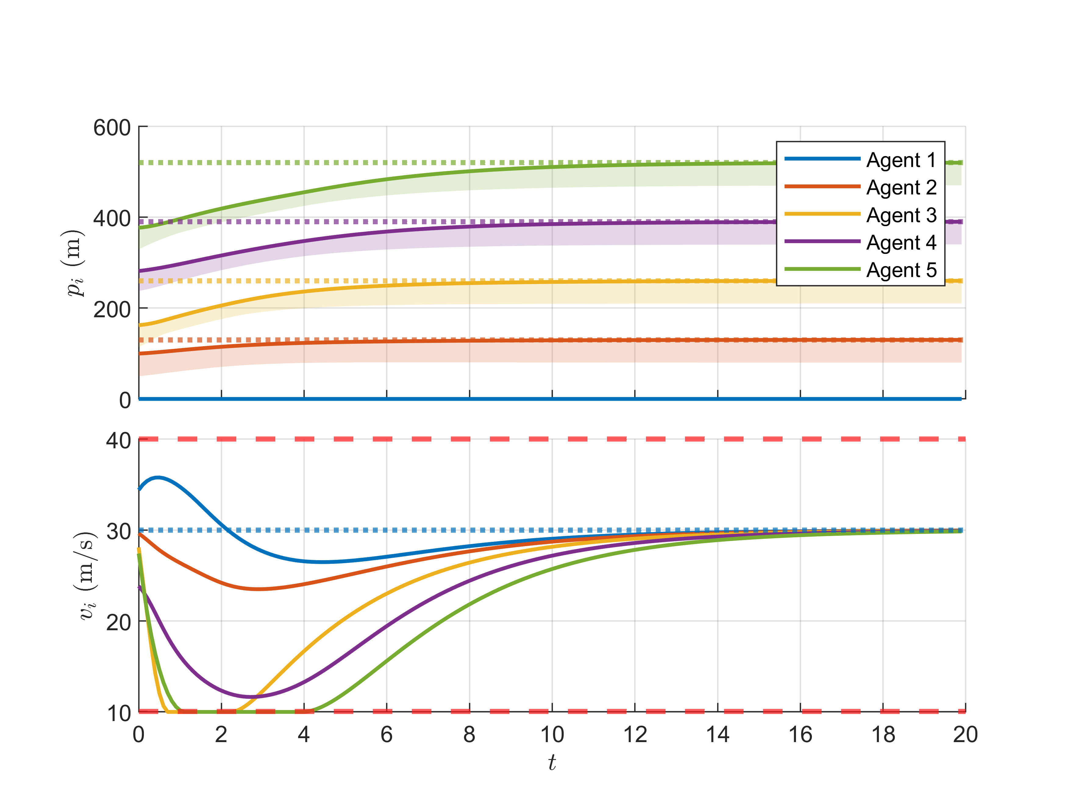
Figure 1: Position with respect to the leading agent and speed for the vehicle platooning scenario. The shaded areas in the first plot represent the safety distance constraints for each agent. The dotted lines represent the position and velocity desired values at steady state. The dashed red lines represent the speed constraints.

V-B Distributed control of interconnected generators

We test the inclusion of the proposed terminal costs on the automatic generation control problem for the power system application considered in [22]. The power system under consideration is composed of $4$ generators interconnected via tie-lines arranged in a line graph with nodes $\mathcal{N}=\{1,...,4\}$ and edges $\mathcal{E}=\{(1,2),(2,3),(3,4)\}$. The models for the dynamics of the generators and of the tie lines linearized around a steady-state reference are the ones in [23], namely

$$\begin{split}A&=\begin{bmatrix}\operatorname{blkdiag}(A^{\text{gen}}_{i})_{i\in\mathcal{N}}&\operatorname{col}(A^{\text{coup}}_{i})_{i\in\mathcal{N}}\\ \operatorname{col}(A^{\text{tie}}_{e})_{e\in\mathcal{E}}&\bm{0}_{3\times 3}\end{bmatrix},\\ A_{i}^{\text{gen}}&=\begin{bmatrix}-D_{i}/M^{a}_{i}&1/M^{a}_{i}&-1/M^{a}_{i}\\ 0&-1/T_{\text{ch},i}&1/T_{\text{ch},i}\\ -1/(R_{i}^{f}T_{G,i})&0&-1/T_{G,i}\end{bmatrix}\\ A^{\text{coup}}_{i}&=\mathcal{B}_{i,:}\otimes\begin{bmatrix}1/M_{i}^{a}\\ 0\\ 0\end{bmatrix}\\ A^{\text{tie}}_{e}&=\mathcal{B}_{:,j}^{\top}\otimes\begin{bmatrix}T_{e},0,0\end{bmatrix}\\ B_{i}&=\delta^{4}_{i}\otimes\begin{bmatrix}0\\ 0\\ 1/T_{G,i}\end{bmatrix},~{}~{}~{}~{}\forall~{}i\in\mathcal{I}.\end{split}$$ (40)

where $\mathcal{B}_{i,:}$ and $\mathcal{B}_{:,j}$ are respectively the $i$-th row and $j$-th column of the incidence matrix for the tie-lines graph. $\delta^{n}_{i}\in\mathbb{R}^{n}$ is a vector with only non-zero element $1$ at index $i$. The model considered has $3$ states for each generator (namely, the angular velocity of the rotating element, the mechanical power applied to the rotating element and the position of the steam valve) and one for each tie line (namely, the power flow). Each agent has control authority over the reference point of their respective governor. The notation for the parameters of the model is as in [24, §A.1], which we refer to for their values and interpretation. The control objective for each agent is to regulate the deviation from the reference angular speed of the generator rotating part and power flow at the tie-line they are connected to, with the exception of agent 1 that does not control the tie line. In numbers, we have

$$\begin{split}R_{i}&=1\quad\forall i\in\{1,2,3,4\};\\ Q_{1}&=\operatorname{blkdiag}(5,\bm{0}_{14\times 14})\\ \forall i&\in\{2,3,4\}:\\ Q_{i}&=\begin{bmatrix}\delta_{i}^{4}(\delta_{i}^{4})^{\top}\otimes\operatorname{diag}(5,0,0)&\bm{0}_{12\times 3}\\ \bm{0}_{3\times 12}&5\delta_{i+1}^{3}(\delta_{i+1}^{3})^{\top}\end{bmatrix}.\end{split}$$ (41)

This application example is chosen as it is observed in [22] that the distributed MPC control architecture (equivalent to the receding-horizon OL-NE without terminal cost in this paper) leads to the system being unstable and thus it is a challenging distributed control problem. We observe that Algorithm 1 converges to an unconstrained infinite-horizon OL-NE feedback synthesis that is not asymptotically stable, thus we could not test the performance of the OL-NE receding horizon controller. Conversely and as expected from Lemma 3, we find a stabilizing infinite-horizon CL-NE using the iterations in [8, Eq. 16]. We test the receding-horizon CL-NE controller which solves the problem in (36) from a randomly generated initial state, and we compare its stabilizing property with respect to the controller which implements (36) without a terminal cost in Figure 2. We estimate a constrained admissible forward invariant set of the form

$$\begin{split}{\mathbb{X}}_{f}^{\text{\tiny{CL}}}=\{x\in\mathbb{X}|\|x\|_{P}^{2}<r\}\end{split}$$ (42)

where $P$ defines a quadratic Lyapunov function for the autonomous system $\bar{A}^{\text{\tiny{CL}}}$ defined as in (34) and $r$ is determined numerically such that the controller $({K}^{\text{\tiny{CL}}}_{i})_{i\in\mathcal{I}}$ is feasible. We observe that the system is asymptotically stable when the initial state is in ${\mathbb{X}}_{f}^{\text{\tiny{CL}}}$. In general, the inclusion of the terminal cost is beneficial for the asymptotic convergence of the closed-loop system.

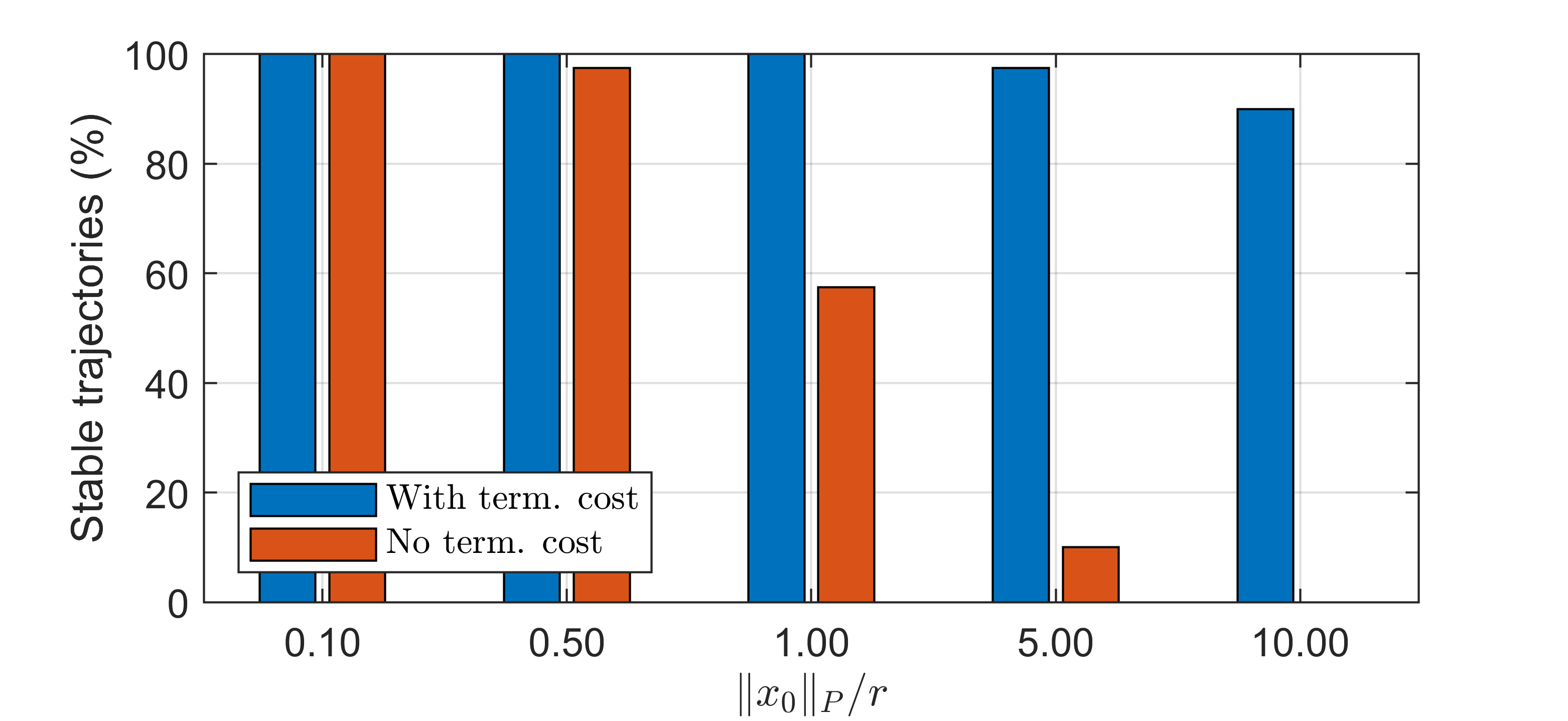
Figure 2: Percentage of asymptotically stable trajectories for the 4-zone power systems in [22] controlled by the receding-horizon CL-NE for different initial states $x_{0}$. $P$ and $r$ define a constraint-admissible forward invariant set as in (42).

VI Conclusion

By using the infinite-horizon cost-to-go over an augmented state-space as terminal cost function, the receding-horizon solution of the constrained finite-horizon open-loop Nash equilibrium inherits the local asymptotic stability property from the stability of the infinite-horizon unconstrained solution. The open-loop Nash equilibrium control inputs can be computed by solving a variational inequality. Instead, the closed-loop Nash equilibrium case requires solving a game with nested equilibrium constraints. Interestingly, with an appropriate relaxation of the equilibrium constraints, the solution of the infinite-horizon problem coincides with the receding-horizon solution of the closed-loop Nash equilibrium problem.

-A Additional results and proofs to Section III-A

Fact 2.

Let ${P}^{\text{\tiny{OL}}}_{i},{K}^{\text{\tiny{OL}}}_{i}$ solve (6). Let $A$ be invertible. Then, (9) holds true.

Proof.

$$\bar{A}^{\text{\tiny{OL}}} {=}A+\textstyle\sum_{i\in\mathcal{I}}B_{i}{K}^{\text{\tiny{OL}}}_{i}$$ (43a)

$${=}A-\textstyle\sum_{i\in\mathcal{I}}S_{i}{P}^{\text{\tiny{OL}}}_{i}\bar{A}^{\text{\tiny{OL}}}$$ (43b)

$$\Leftrightarrow\left(I+\textstyle\sum_{i\in\mathcal{I}}S_{i}{P}^{\text{\tiny{OL}}}_{i}\right)\bar{A}^{\text{\tiny{OL}}}=A$$ (43c)

$$\Leftrightarrow\left(I+\textstyle\sum_{i\in\mathcal{I}}S_{i}{P}^{\text{\tiny{OL}}}_{i}\right)\bar{A}^{\text{\tiny{OL}}}A^{-1}=I,$$ (43d)

thus $(I+\textstyle\sum_{i\in\mathcal{I}}S_{i}{P}^{\text{\tiny{OL}}}_{i})$ is invertible. Left-multiplying (43c) by $(I+\textstyle\sum_{i\in\mathcal{I}}S_{i}{P}^{\text{\tiny{OL}}}_{i})^{-1}$ shows (9). ∎

Proof of Fact 1

(proof of $\eqref{eq:riccati_open_loop}\Rightarrow\eqref{eq:riccati_open_loop_sassano}$). We left-multiply (6a) by $S_{i}A^{-\top}$ and sum over $\mathcal{I}$ to obtain:

$$\begin{split}\mathop{\vbox{\hbox{$\textstyle\sum$}}}\limits_{j\in\mathcal{I}}S_{j}A^{-\top}(Q_{j}-{P}^{\text{\tiny{OL}}}_{j})&=\mathop{\vbox{\hbox{$\textstyle\sum$}}}\limits_{j\in\mathcal{I}}-S_{j}{P}^{\text{\tiny{OL}}}_{j}\bar{A}^{\text{\tiny{OL}}}\\ \overset{\eqref{eq:riccati_open_loop:K},\eqref{eq:definition_S}}{}&{=}\mathop{\vbox{\hbox{$\textstyle\sum$}}}\limits_{j\in\mathcal{I}}B_{j}{K}^{\text{\tiny{OL}}}_{j}.\end{split}$$ (44)

Thus,

$$\begin{split}\bar{A}^{\text{\tiny{OL}}}\overset{\eqref{eq:closed_loop_A_explicit},\eqref{eq:equivalence_freiling_sassano:1}}{}&{=}A+\textstyle\sum_{j\in\mathcal{I}}S_{j}A^{-\top}(Q_{j}-{P}^{\text{\tiny{OL}}}_{j}).\end{split}$$ (45)

By substituting (45) in (6a) we find that (10a) is satisfied and

$${K}^{\text{\tiny{OL}}}_{i}=-R_{i}^{-1}B_{i}^{\top}{P}^{\text{\tiny{OL}}}_{i}(A+\textstyle\sum_{j\in\mathcal{I}}S_{j}A^{-\top}(Q_{j}-{P}^{\text{\tiny{OL}}}_{j}))$$

which reads as (10b) by substituting (10a).

(proof of $\eqref{eq:riccati_open_loop}\Leftarrow\eqref{eq:riccati_open_loop_sassano}$) Substituting (10a) in (10b),

$${K}^{\text{\tiny{OL}}}_{i}=-R_{i}^{-1}B_{i}^{\top}{P}^{\text{\tiny{OL}}}_{i}(A+\textstyle\sum_{h\in\mathcal{I}}S_{h}A^{-\top}(Q_{h}-{P}^{\text{\tiny{OL}}}_{h})).$$ (46)

By substituting (46) and the definition of $S_{i}$ in (7),

$$\bar{A}^{\text{\tiny{OL}}}=A-\mathop{\vbox{\hbox{$\textstyle\sum$}}}\limits_{j\in\mathcal{I}}S_{j}{P}^{\text{\tiny{OL}}}_{j}\big{(}A+\mathop{\vbox{\hbox{$\textstyle\sum$}}}\limits_{h\in\mathcal{I}}S_{h}A^{-\top}(Q_{h}-{P}^{\text{\tiny{OL}}}_{h})\big{)}.$$ (47)

On the other hand, by substituting (10b) in (7),

$$\bar{A}^{\text{\tiny{OL}}}=A+\textstyle\sum_{h\in\mathcal{I}}S_{h}A^{-\top}(Q_{h}-{P}^{\text{\tiny{OL}}}_{h}).$$ (48)

By substituting (48) in (46), one obtains (6b). Finally, by multiplying (10a) with $A^{\top}$ on the left and by substituting (48), one obtains (6a). $\hfill\blacksquare$

Fact 3.

Let $({P}^{\text{\tiny{OL}}}_{i})_{i\in\mathcal{I}},({K}^{\text{\tiny{OL}}}_{i})_{i\in\mathcal{I}}$ solve (10). Then, the conditions in Assumption 3 are satisfied if $\bar{A}^{\text{\tiny{OL}}}$ defined as in (7) is Schur.

Let $({P}^{\text{\tiny{OL}}}_{i})_{i\in\mathcal{I}}$ solve (10) and

$$\bar{P}:=\begin{bmatrix}I\\ \operatorname{col}({P}^{\text{\tiny{OL}}}_{j})_{j\in\mathcal{I}}\end{bmatrix}.$$ (49)

We note that $\mathrm{Im}(\bar{P})$ is complementary to

$$\mathrm{Im}\left(\begin{bmatrix}\bm{0}_{n\times Nn}\\ I_{Nn}\end{bmatrix}\right).$$

It is then sufficient to prove that $\mathrm{Im}(\bar{P})$ is a stable invariant subspace of $H$. By applying the definition of $H$ and $\bar{P}$, we compute

$$H\bar{P}=\begin{bmatrix}A+\sum_{j\in\mathcal{I}}S_{j}A^{-\top}(Q_{j}-{P}^{\text{\tiny{OL}}}_{j})\\ \operatorname{col}(-A^{-\top}(Q_{j}-{P}^{\text{\tiny{OL}}}_{j}))_{j\in\mathcal{I}}\end{bmatrix}.$$ (50)

By substituting (48) and (10a) in (50), one obtains

$$H\bar{P}=\bar{P}\bar{A}^{\text{\tiny{OL}}}$$ (51)

which implies that $\mathrm{Im}(\bar{P})$ is a stable invariant subspace for $H$. It can be verified by right-multiplying (51) by a generic eigenvector of $\bar{A}^{\text{\tiny{OL}}}$ that the eigenvalues of $\bar{A}^{\text{\tiny{OL}}}$ are a subset of the ones of $H$, thus $H$ has at least $n$ eigenvectors strictly in the unit circle and Assumption 3 is satisfied. $\hfill\blacksquare$

-B Additional results and proofs of Section III-B

Let us present a preliminary result to the proof of Lemma 1:

Lemma 4.

Let $({P}^{\text{\tiny{OL}}}_{i},{K}^{\text{\tiny{OL}}}_{i})_{i\in\mathcal{I}}$ solve (6) and let Assumption 1(ii), 2 hold true. Then, for each $i\in\mathcal{I}$, ${P}^{\text{\tiny{OL}}}_{i}={P}^{\text{\tiny{LQR}}}_{i}+\accentset{\sim}{P}_{i}$ where $\accentset{\sim}{P}_{i}$ satisfies

$$\accentset{\sim}{P}_{i}=(\bar{A}^{\text{\tiny{LQR}}}_{i})^{\top}\accentset{\sim}{P}_{i}\bar{A}^{\text{\tiny{OL}}}+(\bar{A}^{\text{\tiny{LQR}}}_{i})^{\top}{P}^{\text{\tiny{LQR}}}_{i}(\textstyle\sum_{j\neq i}B_{j}{K}^{\text{\tiny{OL}}}_{j})$$ (52)

and ${K}^{\text{\tiny{OL}}}_{i}={K}^{\text{\tiny{LQR}}}+\accentset{\sim}{K}_{i}$, where

$$\accentset{\sim}{K}_{i}=-(R_{i}+B_{i}{P}^{\text{\tiny{LQR}}}_{i}B_{i})^{-1}\\ B_{i}^{\top}(\accentset{\sim}{P}_{i}\bar{A}^{\text{\tiny{OL}}}+{P}^{\text{\tiny{LQR}}}_{i}(\textstyle\sum_{j\neq i}B_{j}{K}^{\text{\tiny{OL}}}_{j})).$$ (53)

Proof.

${P}^{\text{\tiny{LQR}}}_{i}$ is symmetric [20, Thm. 22.2], thus (13a) can be written as

$${P}^{\text{\tiny{LQR}}}_{i}=Q_{i}+(\bar{A}^{\text{\tiny{LQR}}}_{i})^{\top}{P}^{\text{\tiny{LQR}}}_{i}A.$$ (54)

Now note:

$$\begin{split}\bar{A}^{\text{\tiny{LQR}}}_{i}{P}^{\text{\tiny{LQR}}}_{i}B_{i}{K}^{\text{\tiny{OL}}}_{i}\overset{\eqref{eq:riccati_open_loop:K}}{}&{=}-\bar{A}^{\text{\tiny{LQR}}}_{i}{P}^{\text{\tiny{LQR}}}_{i}B_{i}R_{i}^{-1}B_{i}^{\top}{P}^{\text{\tiny{OL}}}_{i}\bar{A}^{\text{\tiny{OL}}}\\ \overset{\eqref{eq:lqr:K}}{}&{=}(B_{i}{K}^{\text{\tiny{LQR}}}_{i})^{\top}{P}^{\text{\tiny{OL}}}_{i}\bar{A}^{\text{\tiny{OL}}}.\end{split}$$ (55)

Substituting ${P}^{\text{\tiny{OL}}}_{i}={P}^{\text{\tiny{LQR}}}_{i}+\accentset{\sim}{P}_{i}$ in (6a):

$${P}^{\text{\tiny{LQR}}}_{i}+\accentset{\sim}{P}_{i} =Q_{i}+A^{\top}({P}^{\text{\tiny{LQR}}}_{i}+\accentset{\sim}{P}_{i})\bar{A}^{\text{\tiny{OL}}}$$

$${=}Q_{i}+(\bar{A}^{\text{\tiny{LQR}}}_{i})^{\top}({P}^{\text{\tiny{LQR}}}_{i}+\accentset{\sim}{P}_{i})\bar{A}^{\text{\tiny{OL}}}$$

$$\quad-(B_{i}{K}^{\text{\tiny{LQR}}}_{i})^{\top}{P}^{\text{\tiny{OL}}}_{i}\bar{A}^{\text{\tiny{OL}}}$$

$${=}Q_{i}+(\bar{A}^{\text{\tiny{LQR}}}_{i})^{\top}({P}^{\text{\tiny{LQR}}}_{i}+\accentset{\sim}{P}_{i})\bar{A}^{\text{\tiny{OL}}}$$

$$\quad-\bar{A}^{\text{\tiny{LQR}}}_{i}{P}^{\text{\tiny{LQR}}}_{i}B_{i}{K}^{\text{\tiny{OL}}}_{i}.$$

Subtract (54) from the latter to obtain (52). Let us rewrite (6b) and (13b) respectively as:

$$\begin{multlined}(R_{i}+B_{i}^{\top}{P}^{\text{\tiny{OL}}}_{i}B_{i}){K}^{\text{\tiny{OL}}}_{i}=\\ \qquad-B_{i}^{\top}{P}^{\text{\tiny{OL}}}_{i}(A+\textstyle\sum_{j\neq i}B_{j}{K}^{\text{\tiny{OL}}}_{j});\end{multlined}(R_{i}+B_{i}^{\top}{P}^{\text{\tiny{OL}}}_{i}B_{i}){K}^{\text{\tiny{OL}}}_{i}=\\ \qquad-B_{i}^{\top}{P}^{\text{\tiny{OL}}}_{i}(A+\textstyle\sum_{j\neq i}B_{j}{K}^{\text{\tiny{OL}}}_{j});$$ (58)

$$(R_{i}+B_{i}^{\top}{P}^{\text{\tiny{LQR}}}_{i}B_{i}){K}^{\text{\tiny{LQR}}}_{i}=-B_{i}^{\top}{P}^{\text{\tiny{LQR}}}_{i}A.$$ (59)

Substitute ${P}^{\text{\tiny{OL}}}_{i}={P}^{\text{\tiny{LQR}}}_{i}+\accentset{\sim}{P}_{i}$ in (58):

$$(R_{i}+B_{i}^{\top}{P}^{\text{\tiny{LQR}}}_{i}B_{i}){K}^{\text{\tiny{OL}}}_{i}=\\ -B_{i}^{\top}({P}^{\text{\tiny{OL}}}_{i}(A+\textstyle\sum_{j\neq i}B_{j}{K}^{\text{\tiny{OL}}}_{j})+\accentset{\sim}{P}_{i}B_{i}{K}^{\text{\tiny{OL}}}_{i}).$$

which reads as (53) after subtracting (59). ∎

Proof of Lemma 1

By the Schur property of $\bar{A}^{\text{\tiny{OL}}}$, it follows that any control action that stabilizes $(A,B_{i})$ is stabilizing for $(\widehat{A}_{i},\widehat{B}_{i})$ for all $i$, thus the system in (LABEL:eq:auxiliary_lti_system) is stabilizable. Let $\widehat{A}_{i}z=\lambda z$ for some $\lambda\geq 1$ and $\widehat{C}_{i}z=0$, that is, let $z$ an unstable unobservable mode of $\widehat{A}_{i}$. From the stability of $\bar{A}^{\text{\tiny{OL}}}$, it has to be $z=[x^{\top},{0}^{\top}]^{\top}$ for some $x\in\mathbb{R}^{n}$. Then, $\widehat{A}_{i}z=Ax$ and it has to be $x=0$ by the detectability of $(A,C_{i})$. Consequently, $(\widehat{A}_{i},\widehat{C}_{i})$ is detectable. Following [19, Cor. 13.8], (15a) admits a unique positive semidefinite solution and the corresponding controller is stabilizing. Consider the partition

$$\widehat{P}_{i}=\begin{bmatrix}\widehat{P}_{i}^{1,1}&\widehat{P}_{i}^{1,2}\\ \widehat{P}_{i}^{2,1}&\widehat{P}_{i}^{2,2}\end{bmatrix};\quad\widehat{K}_{i}=[\widehat{K}_{i}^{1},\widehat{K}_{i}^{2}].$$

By expanding (15) for the blocks $\widehat{P}_{i}^{1,1}$, $\widehat{P}_{i}^{2,1}$ and $\widehat{K}_{i}^{1}$, one obtains via straightforward calculations:

$$\widehat{P}_{i}^{1,1} =Q_{i}+A^{\top}\widehat{P}_{i}^{1,1}(A+B_{i}\widehat{K}_{i}^{1})$$ (60a)

$$\widehat{K}_{i}^{1} =-(R_{i}+B_{i}^{\top}\widehat{P}_{i}^{1,1}B_{i})^{-1}B_{i}^{\top}\widehat{P}_{i}^{1,1}A$$ (60b)

$$\widehat{P}_{i}^{2,1} =(\textstyle\sum_{j\neq i}B_{j}{K}^{\text{\tiny{OL}}}_{j})^{\top}\widehat{P}_{i}^{1,1}(A+B_{i}\widehat{K}_{i}^{1})+$$

$$(\bar{A}^{\text{\tiny{OL}}})^{\top}\widehat{P}_{i}^{2,1}(A+B_{i}\widehat{K}_{i}^{1}).$$ (60c)

We note that (60a) and (60b) have the same expression as (13a) and (13b), respectively. From $\widehat{P}_{i}\succcurlyeq 0$, $\widehat{P}_{i}^{1,1}\succcurlyeq 0$. Thus, $\widehat{P}_{i}^{1,1}$ is the unique positive semidefinite solution of (13a) and $\widehat{P}_{i}^{1,1}={P}^{\text{\tiny{LQR}}}_{i}$, $\widehat{K}_{i}^{1}={K}^{\text{\tiny{LQR}}}_{i}$. Thus, by substituting ${P}^{\text{\tiny{LQR}}}_{i}$ and ${K}^{\text{\tiny{LQR}}}_{i}$ in (60c), one obtains that $(\widehat{P}_{i}^{2,1})^{\top}$ must satisfy (52). As (52) is a Stein equation in $\accentset{\sim}{P}_{i}$, its solution is unique following the Schur property of $\bar{A}^{\text{\tiny{LQR}}}_{i}$ and $\bar{A}^{\text{\tiny{OL}}}$ [25, Lemma 2.1]. Thus, $(\widehat{P}_{i}^{2,1})^{\top}=\accentset{\sim}{P}_{i}$.$\hfill\blacksquare$

-C Proofs of Section III-C and III-D

For simplicity, in this section we drop the dependence on $x_{0}$ of $\bm{u}^{*}$, which solves (26), and $\bm{u}^{*}_{\infty}$, defined in (28). We recall that $x^{*}=x(x_{0},\bm{u}^{*})$. We denote the infinite-horizon objective of agent $i$ as

$$J_{i}^{\infty}(u_{i}|x_{0},\bm{u}_{-i})=\tfrac{1}{2}\textstyle\sum_{t=0}^{\infty}\|x[t|x_{0},\bm{u}]\|^{2}_{Q_{i}}+\|u_{i}[t]\|^{2}_{R_{i}}$$ (61)

in contrast to the finite-horizon objective $J_{i}$ in (25).

Proof of Theorem 1

By the invariance of ${\mathbb{X}}_{f}^{\text{\tiny{OL}}}$, $\bm{u}_{\infty}^{*}$ is feasible. To prove it is an OL-NE trajectory, we proceed by contradiction. Assume there exists $v_{i}\in\mathcal{U}_{i}^{\infty}(x_{0},\bm{u}_{\infty,-i}^{*})$ such that

$$J_{i}^{\infty}(v_{i}|x_{0},\bm{u}^{*}_{\infty,-i})<J_{i}^{\infty}(u^{*}_{\infty,i}|x_{0},\bm{u}^{*}_{\infty,-i}).$$ (62)

Let us substitute the definition (28) of $\bm{u}^{*}_{\infty}$ into (61):

$$J_{i}^{\infty}(u^{*}_{\infty,i}|x_{0},\bm{u}^{*}_{\infty,-i})$$

$$=J_{i}^{\infty}\left({u}^{\text{\tiny{OL}}}_{i}(x^{*}[T])|x^{*}[T],\bm{u}^{\text{\tiny{OL}}}_{-i}(x^{*}[T])\right)+$$

$$\quad\tfrac{1}{2}\textstyle\sum_{t=0}^{T-1}\left(\|u^{*}_{T,i}[t]\|^{2}_{R_{i}}+\|x^{*}[t]\|^{2}_{Q_{i}}\right)$$

$${=}V_{i}(x^{*}[T],x^{*}[T])+\tfrac{1}{2}\textstyle\sum_{t=0}^{T-1}\|u^{*}_{i}[t]\|^{2}_{R_{i}}+\|x^{*}[t]\|^{2}_{Q_{i}}$$

$${=}J_{i}\left(u^{*}_{i}|x_{0},\bm{u}^{*}\right).$$

Denote $x_{v}[t]=x[t|x_{0},v_{i},\bm{u}^{*}_{-i}]$ and note:

$$J_{i}^{\infty}(v_{i}|x_{0},\bm{u}^{*}_{\infty,-i})=J_{i}^{\infty}(v_{i}|x_{v}[T],\bm{u}^{\text{\tiny{OL}}}_{-i}(x^{*}[T]))+$$

$$\quad\tfrac{1}{2}\textstyle\sum_{t=0}^{T-1}\|v_{i}[t]\|^{2}_{R_{i}}+\|x_{v}[t]\|^{2}_{Q_{i}}$$

$$\overset{\eqref{eq:V_optimal_xy}}{\geq}V_{i}(x_{v}[T],x^{*}[T])+\tfrac{1}{2}\textstyle\sum_{t=0}^{T-1}\|v_{i}[t]\|^{2}_{R_{i}}+\|x_{v}[t]\|^{2}_{Q_{i}}$$

$$\overset{\eqref{eq:cost_rec_hor_ol}}{=}J_{i}(v_{i}|x_{0},\bm{u}^{*})$$

Thus, (62) contradicts the definition of $\bm{u}^{*}(x_{0})$ in (26). It follows that $\bm{u}^{*}_{\infty}(x_{0})$ is an OL-NE for all $x_{0}\in\mathcal{X}$ and from Definition 2 $\bm{u}^{*}_{\infty}[0|x]=\bm{u}^{*}[0|x]$ is a feedback synthesis of the OL-NE in $\mathcal{X}$.$\hfill\blacksquare$

Proof of Lemma 2

We note that, for any $x_{0}$, by evaluating (24) at optimality for a generic $i\in\mathcal{I}$,

$$\begin{split}&V_{i}(x_{0},x_{0})=\tfrac{1}{2}\|x_{0}\|^{2}_{Q_{i}}+\tfrac{1}{2}\|{K}^{\text{\tiny{OL}}}_{i}x_{0}\|^{2}_{R_{i}}\\ &+V_{i}\large(Ax_{0}+B_{i}{K}^{\text{\tiny{OL}}}_{i}x_{0}+\textstyle\sum_{j\neq i}B_{j}{K}^{\text{\tiny{OL}}}_{j}x_{0},\bar{A}^{\text{\tiny{OL}}}x_{0}\large)\\ &=\tfrac{1}{2}\|x_{0}\|^{2}_{Q_{i}}+\tfrac{1}{2}\|{K}^{\text{\tiny{OL}}}_{i}x_{0}\|^{2}_{R_{i}}+V_{i}(\bar{A}^{\text{\tiny{OL}}}x_{0},\bar{A}^{\text{\tiny{OL}}}x_{0}),\end{split}$$ (63)

where we applied Lemma 4 to substitute ${K}^{\text{\tiny{LQR}}}_{i}+\accentset{\sim}{K}_{i}={K}^{\text{\tiny{OL}}}_{i}$. We proceed by contradiction and thus assume for some $v_{i}\in\mathcal{U}_{i,T}(x^{*}[1],\accentset{\sim}{\bm{u}}_{-i})$

$$J_{i}(v_{i}|x^{*}[1],\accentset{\sim}{\bm{u}})<J_{i}(\accentset{\sim}{u}_{i}|x^{*}[1],\accentset{\sim}{\bm{u}})$$ (64)

and we denote $x_{v}=x(x^{*}[1],v_{i},\accentset{\sim}{\bm{u}}_{-i})$. Define the auxiliary sequence of length $T$

$$\hat{v}_{i}[t]:=\begin{cases}u_{i}^{*}[t]&\text{if}~{}t=0\\ {v}_{i}[t-1]&\text{if}~{}t\in\{1,...,T-1\}.\end{cases}$$ (65)

One can verify that

$$x[t+1|x_{0},\hat{v}_{i},\bm{u}^{*}_{-i}]=x_{v}[t],~{}\forall t\in\mathcal{T}.$$ (66)

As $v_{i}\in\mathcal{U}_{i,T}(x^{*}[1],\accentset{\sim}{\bm{u}}_{-i})$, clearly $\hat{v}_{i}$ is also feasible, that is, $\hat{v}_{i}\in\mathcal{U}_{i,T}(x_{0},{\bm{u}}^{*}_{-i})$. By expanding (25),

$$\begin{split}&J_{i}(v_{i}|x^{*}[1],\accentset{\sim}{\bm{u}})\\ &=V_{i}(x_{v}[T],\bar{A}^{\text{\tiny{OL}}}x^{*}[T])+\tfrac{1}{2}\textstyle\sum_{t=0}^{T-1}\|x_{v}[t]\|^{2}_{Q_{i}}+\|v_{i}[t]\|^{2}_{R_{i}}\\ \overset{\eqref{eq:V_value_function}}{}&{\geq}V_{i}(x_{v}[T-1],x^{*}[T])+\tfrac{1}{2}\textstyle\sum_{t=0}^{T-2}\|x_{v}[t]\|^{2}_{Q_{i}}+\|v_{i}[t]\|^{2}_{R_{i}}\\ \overset{\eqref{eq:state_evol_v_hat}}{}&{=}V_{i}(x[T|x_{0},\hat{v}_{i},\bm{u}^{*}_{-i}],x^{*}[T])\\ &\quad+\tfrac{1}{2}\textstyle\sum_{t=1}^{T-1}\|x[t|x_{0},\hat{v}_{i},\bm{u}^{*}_{-i}]\|^{2}_{Q_{i}}+\|\hat{v}_{i}[t]\|^{2}_{R_{i}}\\ \overset{\eqref{eq:cost_rec_hor_ol}}{}&{=}J_{i}(\hat{v}_{i}|x_{0},\bm{u}^{*})-\tfrac{1}{2}\|x_{0}\|_{Q_{i}}^{2}-\tfrac{1}{2}\|u_{i}^{*}[0]\|^{2}_{R_{i}}.\end{split}$$ (67)

Again from (25) and the definition of $\accentset{\sim}{\bm{u}}$ in (29),

$$\begin{split}&J_{i}(\accentset{\sim}{u}_{i}|x^{*}[1],\accentset{\sim}{\bm{u}})=\tfrac{1}{2}\textstyle\sum_{t=1}^{T-1}\|x^{*}[t]\|^{2}_{Q_{i}}+\|u^{*}_{i}[t]\|^{2}_{R_{i}}\\ &\quad+\tfrac{1}{2}\|x^{*}[T]\|^{2}_{Q_{i}}+\tfrac{1}{2}\|{K}^{\text{\tiny{OL}}}_{i}x^{*}[T]\|^{2}_{R_{i}}\\ &\quad+V_{i}(\bar{A}^{\text{\tiny{OL}}}x^{*}[T],\bar{A}^{\text{\tiny{OL}}}x^{*}[T])\\ \overset{\eqref{eq:evolution_V_nominal}}{}&{=}V_{i}(x^{*}[T],x^{*}[T])+\tfrac{1}{2}\textstyle\sum_{t=1}^{T-1}\|x^{*}[t]\|^{2}_{Q_{i}}+\|u^{*}_{i}[t]\|^{2}_{R_{i}}\\ \overset{\eqref{eq:cost_rec_hor_ol}}{}&{=}J_{i}(u^{*}_{i}|x_{0},\bm{u}^{*})-\tfrac{1}{2}\|x_{0}\|^{2}_{Q_{i}}-\tfrac{1}{2}\|u^{*}_{i}[0]\|^{2}_{R_{i}}.\end{split}$$ (68)

By substituting (67) and (68) in (64), one obtains

$$J_{i}(\hat{v}_{i}|x_{0},\bm{u}^{*})<J_{i}(u^{*}_{i}|x_{0},\bm{u}^{*})$$

which contradicts $\bm{u}^{*}$ being a solution of (26).$\hfill\blacksquare$

Proof of Theorem 2

Let $\bar{C}=\operatorname{col}(C_{i})_{i\in\mathcal{I}}$. It can be shown that $(A,\bar{C})$ is detectable following Assumption 2(ii). $(A,\bar{C})$ is then input/output-to-state-stable [26, Def. 2.22], [27, Prop. 3.3]. As shown in [27, Eq. 12], there exists a function $\Lambda^{\prime}:\mathbb{R}^{n}\to\mathbb{R}_{\geq 0}$ such that, for some $\gamma_{\text{x}},\gamma_{\text{y}},\gamma_{\text{u}},\bar{\gamma}>0$ and for all $x$,

$$\begin{split}&\Lambda^{\prime}(Ax+\textstyle\sum_{i\in\mathcal{I}}B_{i}u_{i})-\Lambda^{\prime}(x)\\ &\leq-\gamma_{\text{x}}\|x\|^{2}+\gamma_{\text{y}}\|\bar{C}x\|^{2}+\gamma_{\text{u}}\|\bm{u}\|^{2}\\ &\leq-\gamma_{\text{x}}\|x\|^{2}+\bar{\gamma}\textstyle\sum_{i\in\mathcal{I}}\large(\|x\|_{Q_{i}}^{2}+\|u_{i}\|_{R_{i}}^{2}\large)\end{split}$$ (69)

where the latter inequality follows from $\|\bar{C}x\|^{2}=\sum_{i}\|x\|_{Q_{i}}^{2}$ and the equivalence of norms. By applying an equivalence result for storage functions [26, Theorem B.53], there exists then $\Lambda:\mathbb{R}^{n}\to\mathbb{R}_{\geq 0}$ and a positive definite function $\rho$ such that

$$\Lambda(Ax+\textstyle\sum_{i\in\mathcal{I}}B_{i}u_{i})-\Lambda(x)\\ \leq-\rho(\|x\|)+\textstyle\sum_{i\in\mathcal{I}}\large(\|x\|_{Q_{i}}^{2}+\|u_{i}\|_{R_{i}}^{2}\large).$$ (70)

Consider the candidate Lyapunov function

$$V(x_{0})=\Lambda(x_{0})+\textstyle\sum_{i\in\mathcal{I}}J_{i}(u_{i}^{*}(x_{0})|x,\bm{u}^{*}(x_{0}))$$ (71)

where $\bm{u}^{*}(x_{0})$ solves (26). Let $x^{+}$ be the state of the closed-loop system after one timestep, that is, $x^{+}=x[1|x_{0},\bm{u}^{*}]$. Define the shifted input sequence $\accentset{\sim}{\bm{u}}$ as in (29), which solves (26) with initial state $x^{+}$ following Lemma 2 and Assumption 5. Then,

$$\begin{split}&V(x^{+})-\Lambda(x^{+})=\mathop{\vbox{\hbox{$\textstyle\sum$}}}\limits_{i\in\mathcal{I}}J_{i}(\accentset{\sim}{u}_{i}|x^{+},\accentset{\sim}{\bm{u}})\\ &=\mathop{\vbox{\hbox{$\textstyle\sum$}}}\limits_{i\in\mathcal{I}}\Big{(}V_{i}(x[T|x^{+},\accentset{\sim}{\bm{u}}],x[T|x^{+},\accentset{\sim}{\bm{u}}])\\ &\quad+\mathop{\vbox{\hbox{$\textstyle\sum$}}}\limits_{t=0}^{T-1}\|x[t|x^{+},\accentset{\sim}{\bm{u}}]\|^{2}_{Q_{i}}+\|\accentset{\sim}{u}_{i}[t]\|_{R_{i}}^{2}\Big{)}\\ \overset{\eqref{eq:shifted_sol}}{}&{=}\mathop{\vbox{\hbox{$\textstyle\sum$}}}\limits_{i\in\mathcal{I}}\Big{(}V_{i}(\bar{A}^{\text{\tiny{OL}}}x[T|x_{0},\bm{u}^{*}],\bar{A}^{\text{\tiny{OL}}}x[T|x_{0},\bm{u}^{*}])\\ &\quad+\|x[T|x_{0},\bm{u}^{*}]\|_{Q_{i}}^{2}+\|{K}^{\text{\tiny{OL}}}_{i}x[T|x_{0},\bm{u}^{*}]\|_{R_{i}}^{2}\\ &\quad+\mathop{\vbox{\hbox{$\textstyle\sum$}}}\limits_{t=0}^{T-2}\|x[t+1|x_{0},\bm{u}^{*}]\|^{2}_{Q_{i}}+\|u_{i}^{*}[t+1]\|_{R_{i}}^{2}\Big{)}\\ \overset{\eqref{eq:evolution_V_nominal}}{}&{=}\mathop{\vbox{\hbox{$\textstyle\sum$}}}\limits_{i\in\mathcal{I}}\big{(}V_{i}(x[T|x_{0},\bm{u}^{*}],x[T|x_{0},\bm{u}^{*}])\\ &\quad+\mathop{\vbox{\hbox{$\textstyle\sum$}}}\limits_{t=1}^{T-1}\|x[t|x_{0},\bm{u}^{*}]\|^{2}_{Q_{i}}+\|u_{i}^{*}[t]\|_{R_{i}}^{2}\big{)}\\ \overset{\eqref{eq:cost_rec_hor_ol}}{}&{=}\mathop{\vbox{\hbox{$\textstyle\sum$}}}\limits_{i\in\mathcal{I}}\Big{(}J_{i}(u_{i}^{*}|x_{0},\bm{u}^{*})-\|x_{0}\|^{2}_{Q_{i}}-\|u_{i}^{*}[0]\|_{R_{i}}^{2}\Big{)}\\ \overset{\eqref{eq:lyapunov_function}}{}&{=}V(x_{0})-\Lambda(x_{0})-\mathop{\vbox{\hbox{$\textstyle\sum$}}}\limits_{i\in\mathcal{I}}\Big{(}\|x_{0}\|^{2}_{Q_{i}}+\|u_{i}^{*}[0]\|_{R_{i}}^{2}\Big{)}.\end{split}$$ (72)

We rearrange (72) to obtain

$$\begin{split}&V(x^{+})-V(x_{0})\\ &{=}\Lambda(x^{+})-\Lambda(x_{0})-\mathop{\vbox{\hbox{$\textstyle\sum$}}}\limits_{i\in\mathcal{I}}\|x_{0}\|^{2}_{Q_{i}}+\|u_{i}^{*}[0]\|_{R_{i}}^{2}\\ \overset{\eqref{eq:ioss_lyap}}{}&{\leq}-\rho(\|x_{0}\|).\end{split}$$ (73)

From the invariance of ${\mathbb{X}}_{f}^{\text{\tiny{OL}}}$, $\bar{A}^{\text{\tiny{OL}}}x\in{\mathbb{X}}_{f}^{\text{\tiny{OL}}}$. As $\bar{A}^{\text{\tiny{OL}}}x$ is the terminal state for $\accentset{\sim}{\bm{u}}$ with initial state $x^{+}$ we obtain from the definition of $\mathcal{X}$ that $x^{+}\in\mathcal{X}$. Thus, $\mathcal{X}$ is invariant for the closed-loop system. By an induction argument, we conclude that $V$ is a Lyapunov function for the closed-loop system.∎

Proof of Proposition 2

In this proof, we will treat finite sequences as column vectors, that is, $u_{i}=\operatorname{col}(u_{i}[t])_{{t\in\mathcal{T}}}$, $x=\operatorname{col}(x[t])_{t\in\mathcal{T}^{+}}$. Let $\bm{u}^{*}$ solve $\mathrm{VI}(F(\cdot|x_{0}),\bm{\mathcal{U}}_{T}(x_{0}))$. Let us denote the last row block of $\Gamma_{i}$, for all $i$, as follows:

$$\hat{\Gamma}_{i}:=\begin{bmatrix}A^{T-1}B_{i}&A^{T-2}&\dots&&B_{i}\end{bmatrix}.$$

We can rewrite the state evolution as:

$$\begin{split}x(x_{0},u_{i},\bm{v}_{-i})&=\Theta x_{0}+\Gamma_{i}u_{i}+\textstyle\sum_{j\neq i}\Gamma_{j}v_{j}.\end{split}$$ (74)

Using (74) we find the following expression for the terminal states appearing in (25)

$$\begin{split}x[T|x_{0},\bm{v}]&=A^{T}x_{0}+\hat{\Gamma}_{i}v_{i}+\textstyle\sum_{j\neq i}\hat{\Gamma}_{j}v_{j}\\ x[T|x_{0},u_{i},\bm{v}_{-i}]&=A^{T}x_{0}+\hat{\Gamma}_{i}u_{i}+\textstyle\sum_{j\neq i}\hat{\Gamma}_{j}v_{j}.\end{split}$$ (75)

Substituting (74) and (75) in (25), one obtains with straightforward calculations:

$$\begin{split}&J_{i}(u_{i}|x_{0},\bm{v})=u_{i}^{\top}\hat{\Gamma}_{i}^{\top}(\tfrac{1}{2}{P}^{\text{\tiny{LQR}}}_{i}\hat{\Gamma}_{i}u_{i}+\accentset{\sim}{P}_{i}\hat{\Gamma}_{i}v_{i})\\ &~{}~{}+{u}_{i}^{\top}\hat{\Gamma}_{i}^{\top}{P}^{\text{\tiny{OL}}}_{i}(A^{T}x_{0}+\textstyle\sum_{j\neq i}\hat{\Gamma}_{j}{v}_{j})\\ &~{}~{}+\tfrac{1}{2}{u}_{i}^{\top}(\bar{R}_{i}+\Gamma_{i}^{\top}(I_{T}\otimes{Q}_{i})\Gamma_{i}){u}_{i}\\ &~{}~{}+{u}_{i}^{\top}\Gamma_{i}^{\top}(I_{T}\otimes{Q}_{i})(\Theta x_{0}+\textstyle\sum_{j\neq i}\Gamma_{j}{v}_{j})+f(x_{0},\bm{v})\end{split}$$ (76)

where $f$ contains all the additive terms that do not depend on $u_{i}$. By deriving the latter with respect to $u_{i}$, we find

$$F(\bm{u}|x_{0})=\operatorname{col}(\nabla_{u_{i}}J_{i}(u_{i}|x_{0},\bm{v})|_{\bm{v}=\bm{u}})_{i\in\mathcal{I}}.$$

Furthermore, $J_{i}(\cdot|x_{0},\bm{v})$ is convex for every $x_{0},\bm{v}$, because ${P}^{\text{\tiny{LQR}}}_{i}\succcurlyeq 0$, $Q_{i}\succcurlyeq 0$, $R\succ 0$. Thus, by the definition of VI solution, for any $u_{i}\in\mathcal{U}_{i,T}(x_{0},\bm{u}^{*}_{-i})$:

$$0 \leq F(\bm{u}^{*}|x_{0})^{\top}\left(\operatorname{col}(u_{i},\bm{u}^{*}_{-i})-\bm{u}^{*}\right)$$

$$=\nabla_{u_{i}}J_{i}(u^{*}_{i}|x_{0},\bm{v})|_{\bm{v}=\bm{u}^{*}}^{\top}(u_{i}-u_{i}^{*})$$

$$\leq J_{i}(u_{i}|x_{0},\bm{u}^{*})-J_{i}(u^{*}_{i}|x_{0},\bm{u}^{*}),$$

which shows that $\bm{u}^{*}$ solves the problem in (26). $\hfill\blacksquare$

-D Additional results and proofs of Section IV

Before proving Theorem 3, let us show that the CL-NE satisfies an optimality principle:

Lemma 5.

Let $({P}^{\text{\tiny{CL}}}_{i},{K}^{\text{\tiny{CL}}}_{i})_{i\in\mathcal{I}}$ satisfy (33). Then, for all $i\in\mathcal{I}$,

$$\tfrac{1}{2}\|x\|_{{P}^{\text{\tiny{CL}}}_{i}}^{2}=\min_{u_{i}\in\mathbb{R}^{m}}~{}\tfrac{1}{2}\large(\|x\|^{2}_{Q_{i}}+\|u_{i}\|^{2}_{R_{i}}\\ +\|\bar{A}^{\text{\tiny{CL}}}_{-i}x+B_{i}u_{i}\|^{2}_{{P}^{\text{\tiny{CL}}}_{i}}\large)$$ (77)

and the minimum is achieved by ${K}^{\text{\tiny{CL}}}_{i}x$.

Proof.

Let us rewrite (33b) as

$${K}^{\text{\tiny{CL}}}_{i}=-(R_{i}+B_{i}^{\top}{P}^{\text{\tiny{CL}}}_{i}B_{i})^{-1}B_{i}^{\top}{P}^{\text{\tiny{CL}}}_{i}\bar{A}^{\text{\tiny{CL}}}_{-i}.$$

By setting the gradient of (77) to $0$ and comparing the resulting equation with the latter, one can see that the minimum is achieved by ${K}^{\text{\tiny{CL}}}_{i}x$. By substituting $u_{i}={K}^{\text{\tiny{CL}}}_{i}x$ in (77), the minimum of (77) is

$$\|x\|^{2}_{Q_{i}}+({K}^{\text{\tiny{CL}}}_{i}x)^{\top}R_{i}{K}^{\text{\tiny{CL}}}_{i}x+(\bar{A}^{\text{\tiny{CL}}}x)^{\top}{P}^{\text{\tiny{CL}}}_{i}\bar{A}^{\text{\tiny{CL}}}x\overset{\eqref{eq:riccati_CL:K}}{=}$$

$$\|x\|^{2}_{Q_{i}}-({K}^{\text{\tiny{CL}}}_{i}x)^{\top}B_{i}^{\top}{P}^{\text{\tiny{CL}}}_{i}\bar{A}^{\text{\tiny{CL}}}x+(\bar{A}^{\text{\tiny{CL}}}x)^{\top}{P}^{\text{\tiny{CL}}}_{i}\bar{A}^{\text{\tiny{CL}}}x=$$

$$\|x\|^{2}_{Q_{i}}+x^{\top}(\bar{A}^{\text{\tiny{CL}}}-B_{i}{K}^{\text{\tiny{CL}}}_{i})^{\top}{P}^{\text{\tiny{CL}}}_{i}\bar{A}^{\text{\tiny{CL}}}x\overset{\eqref{eq:riccati_CL:P}}{=}\|x\|_{{P}^{\text{\tiny{CL}}}_{i}}^{2}.$$

∎

Proof of Theorem 3

We rewrite the minimization in (36b) as

$$\min_{u_{i}\in\mathcal{S}_{T-1}^{m}}\tfrac{1}{2}\big{\{}\textstyle\sum_{\tau=0}^{T-2}\|x[\tau]\|_{Q_{i}}^{2}+\|u_{i}[\tau]\|_{R_{i}}^{2}\\ +\min_{u_{i}[T-1]\in\mathbb{R}^{m}}\large(\|x[T-1]\|_{Q_{i}}^{2}+\|u_{i}[T-1]\|_{R_{i}}^{2}\\ +\|x[T]\|_{{P}^{\text{\tiny{CL}}}_{i}}^{2}\large)\big{\}}.$$ (78)

By substituting the constraint (36d) in (78) and by applying Lemma 5, the inner minimization in (78) is solved by $u_{i}^{*}[T-1]={K}^{\text{\tiny{CL}}}_{i}x[T-1]$. Substituting (77) in the latter, we obtain

$$\begin{split}&\min_{u_{i}\in\mathcal{S}_{T-1}^{m}}\tfrac{1}{2}\big{(}\|x[T-1]\|_{{P}^{\text{\tiny{CL}}}_{i}}^{2}+\mathop{\vbox{\hbox{$\textstyle\sum$}}}\limits_{\tau=0}^{T-2}\|x[\tau]\|_{Q_{i}}^{2}+\|u_{i}[\tau]\|_{R_{i}}^{2}\big{)}.\end{split}$$

By repeating the reasoning backwards in time and substituting the constraint (36c), (36b) becomes

$$\begin{split}\min_{u_{i}[0]\in\mathbb{R}^{m}}\tfrac{1}{2}&\big{(}\|x[0]\|_{Q_{i}}^{2}+\|u_{i}[0]\|_{R_{i}}^{2}\\ &+\big{\|}Ax[0]+\textstyle\sum_{j\in\mathcal{I}}B_{j}u_{j}[0]\big{\|}_{{P}^{\text{\tiny{CL}}}_{i}}^{2}\big{)}.\end{split}$$ (79)

If $u_{j}[0]={K}^{\text{\tiny{CL}}}_{j}x[0]$ for all $j\in\mathcal{I}_{-i}$, the minimum is obtained by $u_{i}^{*}[0]={K}^{\text{\tiny{CL}}}_{i}x[0]$ following Lemma 5. Thus, $\bm{u}^{*}$ is a NE. $\hfill\blacksquare$

References

• [1] M. Wang, Z. Wang, J. Talbot, J. C. Gerdes, and M. Schwager, “Game-Theoretic Planning for Self-Driving Cars in Multivehicle Competitive Scenarios,” IEEE Transactions on Robotics, vol. 37, pp. 1313–1325, Aug. 2021.
• [2] R. Spica, E. Cristofalo, Z. Wang, E. Montijano, and M. Schwager, “A Real-Time Game Theoretic Planner for Autonomous Two-Player Drone Racing,” IEEE Transactions on Robotics, vol. 36, pp. 1389–1403, Oct. 2020.
• [3] Y. Theodor and U. Shaked, “Output-feedback mixed ${H}_{\infty}$ $H_{2}$ control - a dynamic game approach,” International Journal of Control, vol. 64, pp. 263–279, May 1996.
• [4] S. Hall, L. Guerrini, F. Dörfler, and D. Liao-McPherson, “Game-theoretic Model Predictive Control for Modelling Competitive Supply Chains,” Jan. 2024. arXiv:2401.09853 [cs, eess].
• [5] S. Hall, G. Belgioioso, D. Liao-McPherson, and F. Dorfler, “Receding Horizon Games with Coupling Constraints for Demand-Side Management,” in 61st Conference on Decision and Control (CDC), pp. 3795–3800, IEEE, 2022.
• [6] T. Başar and G. J. Olsder, Dynamic noncooperative game theory. No. 23 in Classics in applied mathematics, Philadelphia: SIAM, 2nd ed ed., 1999.
• [7] A. Monti, B. Nortmann, T. Mylvaganam, and M. Sassano, “Feedback and Open-Loop Nash Equilibria for LQ Infinite-Horizon Discrete-Time Dynamic Games,” SIAM Journal on Control and Optimization, vol. 62, pp. 1417–1436, June 2024.
• [8] B. Nortmann, A. Monti, M. Sassano, and T. Mylvaganam, “Nash Equilibria for Linear Quadratic Discrete-time Dynamic Games via Iterative and Data-driven Algorithms,” IEEE Transactions on Automatic Control, pp. 1–15, 2024.
• [9] A. Haurie, J. B. Krawczyk, and G. Zaccour, Games and Dynamic Games, vol. 1 of World Scientific-Now Publishers Series in Business. World Scientific, Mar. 2012.
• [10] F. Facchinei, A. Fischer, and V. Piccialli, “On generalized Nash games and variational inequalities,” Operations Research Letters, vol. 35, pp. 159–164, Mar. 2007.
• [11] F. Facchinei and J.-S. Pang, Finite-dimensional variational inequalities and complementarity problems. Springer, 2007.
• [12] F. Laine, D. Fridovich-Keil, C.-Y. Chiu, and C. Tomlin, “The Computation of Approximate Generalized Feedback Nash Equilibria,” SIAM Journal on Optimization, vol. 33, pp. 294–318, 2023.
• [13] S. Hall, D. Liao-McPherson, G. Belgioioso, and F. Dörfler, “Stability Certificates for Receding Horizon Games,” Apr. 2024. arXiv:2404.12165 [cs, eess].
• [14] W. B. Dunbar and R. M. Murray, “Distributed receding horizon control for multi-vehicle formation stabilization,” Automatica, vol. 42, pp. 549–558, Apr. 2006.
• [15] W. B. Dunbar, “Distributed Receding Horizon Control of Dynamically Coupled Nonlinear Systems,” IEEE Transactions on Automatic Control, vol. 52, pp. 1249–1263, July 2007.
• [16] M. Farina and R. Scattolini, “Distributed predictive control: A non-cooperative algorithm with neighbor-to-neighbor communication for linear systems,” Automatica, vol. 48, no. 6, pp. 1088–1096, 2012.
• [17] G. Freiling, G. Jank, and H. Abou-Kandil, “Discrete-Time Riccati Equations in Open-Loop Nash and Stackelberg Games,” European Journal of Control, 1999.
• [18] S. Van Huffel, V. Sima, A. Varga, S. Hammarling, and F. Delebecque, “High-performance numerical software for control,” IEEE Control Systems Magazine, vol. 24, pp. 60–76, 2004.
• [19] K. Zhou, J. Doyle, and K. Glover, Robust and optimal control. Prentice Hall, 1996.
• [20] J. P. Hespanha, Linear systems theory. Princeton Oxford: Princeton University Press, second edition ed., 2018.
• [21] S. Shi and M. Lazar, “On distributed model predictive control for vehicle platooning with a recursive feasibility guarantee,” IFAC-PapersOnLine, vol. 50, pp. 7193–7198, July 2017.
• [22] A. Venkat, I. Hiskens, J. Rawlings, and S. Wright, “Distributed MPC Strategies With Application to Power System Automatic Generation Control,” IEEE Transactions on Control Systems Technology, vol. 16, pp. 1192–1206, Nov. 2008.
• [23] A. J. Wood, B. F. Wollenberg, and G. B. Sheblé, Power Generation, Operation and Control. John Wiley & Sons, 2014.
• [24] A. N. Venkat, Distributed Model Predictive Control: Theory and Applications. PhD thesis, UW-Madison, 2006.
• [25] T. Jiang and M. Wei, “On solutions of the matrix equations $X-AXB=C$ and $X-AXB=C$,” Linear Algebra and its Applications, vol. 367, pp. 225–233, July 2003.
• [26] J. B. Rawlings, D. Q. Mayne, and M. Diehl, Model predictive control: theory, computation, and design. Nob Hill Publishing, 2nd ed., 2017.
• [27] C. Cai and A. R. Teel, “Input–output-to-state stability for discrete-time systems,” Automatica, vol. 44, pp. 326–336, 2008.