Strongly interacting fermions are non-trivial yet non-glassy
Abstract
Random spin systems at low temperatures are glassy and feature computational hardness in finding low-energy states. We study the random all-to-all interacting fermionic Sachdev–Ye–Kitaev (SYK) model and prove that, in contrast, (I) the low-energy states have polynomial circuit depth, yet (II) the annealed and quenched free energies agree to inverse-polynomially low temperatures, ruling out a glassy phase transition in this sense. These results are derived by showing that fermionic and spin systems significantly differ in their commutation index, which quantifies the non-commutativity of Hamiltonian terms. Our results suggest that low-temperature strongly interacting fermions, unlike spins, belong in a classically nontrivial yet quantumly easy phase.
I Introduction
Simulating ground and thermal state properties of quantum systems is a key application of future quantum computers [1, 2, 3, 4, 5, 6, 7]. Nevertheless, the search for particular, favorable instances that are quantumly easy and classically hard is not clear-cut [8]. A challenge is that current quantum computers are limited in quality and size, requiring the community to rely on theoretical arguments to give computational separations. However, the ground states for standard few-body quantum spin models can be QMA-hard (as classical spin models are NP-hard) in the worst case [9, 10, 11]; in the average case, random classical and quantum spin models exhibit glassy physics where computational hardness may arise [12, 13]. To give an efficient quantum algorithm for low-temperature states, one must carefully avoid these instances.
Most chemical and condensed matter systems involve fermionic degrees of freedom, not spins. Of particular importance in quantum chemistry is the strongly interacting regime, where Gaussian states do not give good approximations to the ground state and the Hartree–Fock method fails [14]. This has been proposed as a promising regime in which to apply quantum computers to achieve quantum advantage [3]. The Sachdev–Ye–Kitaev (SYK) Hamiltonian provides a natural model for strongly interacting fermions [15, 16, 17]. As a counterpart to random spins, it is a random Hamiltonian consisting of all-to-all -body Majorana fermions:
| (1) |
where and are i.i.d. standard Gaussian random variables.
While the 4-body fermionic ground state problem can be just as hard as spin models in the worst case (NP-hard) [18], average-case fermionic systems appear to have qualitatively different physics and perhaps computational complexity than spin systems [19, 20, 13]. Extensive heuristic calculations (such as large-N expansions) together with numerical evidence indicate that the SYK model resembles a thermalizing chaotic system, not a frozen spin-glass as occurs with few-body quantum spin systems [13, 21]. However, rigorous proofs that go beyond the physical arguments have been very limited [19, 22].
In this Letter, we study the strongly interacting SYK model and give quantitative evidence that random, all-to-all connected fermionic systems have a classically non-trivial yet non-glassy thermal state at constant temperatures. In contrast, these two properties are false for disordered spin systems [23, 24]. Remarkably, the proofs of both main results rely on the same quantity, the commutation index [25]. This quantity pinpoints a crucial and often overlooked distinction between fermionic and spin Hamiltonians: low-degree fermionic monomials have a very different commutation structure than low-weight Pauli operators. The commutation index captures this difference, quantifying the fundamental distinction in the physics of local spin systems and local fermionic systems. This disparity, we argue, is the origin of a potential quantum advantage in simulating strongly interacting fermionic systems.
More precisely, we first show that all low-energy states (including constant-temperature thermal states) of the SYK model have high circuit complexity (‘classically non-trivial’):
Theorem I.1 (Low energy states are classically nontrivial).
Consider the degree- SYK model . With high probability, the maximum energy is , yet any state such that
| (2) |
has circuit complexity
| (3) |
That is, low-energy states of the SYK model are highly entangled and require many parameters to describe; simple classical ansatzes, such as Gaussian states, must fail. In comparison, local quantum spin systems are known to have efficiently computable product state approximations to the ground state [24] and thus, in this sense, have ‘trivial’ states that achieve a constant-factor approximation of the ground state energy.
Second, we show that the quenched free energy of the SYK model agrees with the annealed free energy even at very low temperatures (‘non-glassy’), formalizing and strengthening previous results of this nature [26, 13, 21, 27].111In particular, Ref. [13] showed that the SYK model is consistent with an annealed approximation, and here we prove that the annealed approximation holds. Here, the free energy is normalized such that corresponds to constant physical temperature.
Theorem I.2 (Annealed at low temperatures).
Consider the partition function of the degree- SYK model . Then, we have:
| (4) |
The quantitative agreement of the two free energies at (inverse-polynomially) low temperatures strikes a stark contrast with disordered spin systems: the SYK model does not experience a ‘glass’ phase transition in the sense of quenched-vs.-annealed free energy. For classical spin Hamiltonians, it is known that the annealed free energy fails to agree with the quenched free energy at constant temperatures where the Hamiltonian is in its glassy phase and algorithmic hardness arises (see Appendix A); disordered quantum spin systems undergo a similar transition at constant temperature [23]. The lack of a glass transition for the SYK model suggests that there may be no algorithmic obstructions to preparing low-temperature states of the model on a quantum computer, but we do not prove this claim. We leave finding such an efficient quantum algorithm for future work.
Finally, we study the ground state energy of the SYK model as a function of the locality , as an extension of Theorem I.1 with potentially large .
Theorem I.3 (Lower bounding the norm with -dependence).
With high probability over the disorder it holds that the maximum energy of the degree- SYK model is .
We show a similar scaling for -body quantum spin glasses. To our knowledge this is the first lower bound on the maximum eigenvalue which scales as ; for both models only the scaling at constant was previously known [22, 19, 28, 29]. Our lower bound technique relies on a measure of anticommutation which we call the commutation degree, which counts the maximum number of operators that anti-commute with any given operator in the Hamiltonian. Interestingly, the commutation degree does not distinguish between local spin operators and local fermionic operators.
Background and related work. The SYK model is a canonical instance of a chaotic Hamiltonian [15, 16, 17] with related models studied as far back as [30, 31]. For even , the SYK model has a Gaussian spectrum [22] and heuristics from physics indicate that the expected maximum energy of the SYK model scales as for even [32, 33, 19]. However, the only rigorous result we are aware of with explicit constants is an upper bound of [22]. Though Gaussian state approximation algorithms exist for fermionic systems [24, 28], it is known that for the SYK model with , Gaussian states cannot achieve constant factor approximations to the maximum energy [34]. Separate from the SYK model, so-called no low-energy trivial states (NLTS) theorems rule out constant factor approximations to ground energies with low depth circuits in worst-case settings [35, 36]. For random nonlocal Hamiltonians, [37] shows a circuit lower bound for sparse, sampled Pauli models using a similar technique as in the proof of I.1, where the commutation index is much more straightforward to calculate.
The commutation index has connections to other areas of quantum information theory and Hamiltonian complexity. In [38, 39], the commutation index (there termed the generalized radius) is used to study generalized Heisenberg uncertainty relations. Related to our work, [19] use the commutation index to analyze the performance of sum-of-squares relaxations of the SYK model and prove the instance of II.1, giving as well an algorithm verifying energy for . [29] demonstrates that product states maximize the energy variance for random quantum spin Hamiltonians. Finally, the commutation index appears in quantum learning theory, where it provides a sample-complexity lower bound on how many copies of the state are required to learn the expectation values of a set of operators via shadow tomography [40, 25].
II Commutation structure of local operators
The commutation index of a given set of operators is defined to be [25]:
| (5) |
When all the commutation index takes values . Roughly, a more ‘commuting’ set of observables gives a larger value of . For example, if the operators in are all mutually commuting Pauli operators, choosing to be a simultaneous eigenstate gives .
The commutation index has strong implications for the physics of the model with Gaussian coefficients . Crucially, it controls the concentration of the eigenvalues of :
| (6) |
This holds since governs how sensitive the energy of any given state is when varying the couplings of the model:
| (7) |
Our key observation is that the commutation index of the set of degree- Majorana operators is very small:
Theorem II.1.
Let be the set of degree- Majorana operators on fermionic modes. Then for any constant, even :
| (8) |
The decay with system size is unique to the fermionic setting—for local Pauli operators, is constant with respect to (see Table 1). This behaviour was first conjectured in [19] to our knowledge, and we establish the conjecture—including the setting when scales with —in Section B.4.
| Set | Commutation index |
|---|---|
| Commuting | |
| -local Paulis | (B.1) |
| Degree- Majoranas | (II.1) |
| All Paulis | [40, Lemma 5.8] |
The proof of II.1 involves constructing the commutation graph whose vertices correspond to operators with edges between operators if and only if they anti-commute. The commutation index can be upper bounded by , where is the so-called Lovász theta function of the commutation graph. The Lovász theta function can be efficiently computed via a semi-definite program [41]. For the SYK Hamiltonian, is the graph of a certain Johnson association scheme [42].
In the course of writing our results we became aware of Ref. [43], which also establishes the necessary results on the Lovász theta function of Johnson association schemes. Our results use different proof techniques and determine the explicit -dependence of the constant in Eq. (8), which was not derived in [43].
III Circuit lower bound for the SYK model
An almost direct consequence of a decaying commutation index is a lower bound on the complexity of any ansatz in constructing near-ground states. For any random Hamiltonian with i.i.d. Gaussian coefficients , the commutation index characterizes the maximum variance of the energy for an arbitrary fixed state . Standard concentration bounds then imply that the probability a state has energy is bounded as . This concentration is so strong that one can bound the maximum energy over extremely large sets of states (or -nets of infinite sets) via a simple union bound argument with high probability over the disorder. In particular, we obtain a lower bound on the cardinality of the class of ansatzes needed to achieve a given energy .
Specializing to the SYK model via I.1, we summarize the implications of this result for various classes of states in Table 2. For instance, we show that all states that achieve a constant (i.e., ) approximation ratio with the SYK ground state energy have a quantum circuit depth of . In contrast, product states give constant factor approximations to the ground state energy for any local spin Hamiltonian (see Appendix E for a short proof). Our argument also extends to classical ansatzes. For instance, tensor network methods require a bond dimension that grows polynomially with to construct near-ground states [44, 45]. Similarly, popular methods based on neural quantum states [46, 47, 48, 49, 50] need at least parameters to construct near-ground states for the standard SYK model, implying a fully connected network must have layer width that grows as .
| Ansatz | Circuit complexity∗ |
|---|---|
| Quantum circuit with gates | |
| MPS with bond dimension | |
| Neural network with parameters | |
| ∗min. complexity to achieve energy w.h.p. | |
Our circuit lower bound is related to the study of ‘no low-energy trivial states’ (NLTS) Hamiltonians, whose existence was conjectured in [51] and resolved in [35, 36]. However, the settings are not strictly comparable: our instances are random (average-case), whereas NLTS is formalized for worst-case bounded interaction instances of Hamiltonians. The randomness allows us to prove stronger statements in two ways. First, our circuit lower bounds hold for states at any constant temperature, rather than for states below some energy threshold. Second, we can achieve arbitrary polynomial circuit depth lower bounds, whereas current constructions of NLTS only give a logarithmic depth lower bound. See Appendix E for more discussion.
IV Annealed approximation for the SYK model
The commutation index also has direct implications for the concentration of various physical properties of interest around their disordered expectation. One manifestation of this is in the relation between the quenched and annealed free energies:
| (9) |
where is the partition function of the model at an inverse temperature . The quenched free energy assumes the disorder induced by the random couplings is fixed when averaging over thermal fluctuations; the annealed free energy treats these fluctuations on an equal footing. While the two quantities agree at high temperature, at low temperature the latter is incapable of accounting for frustration induced by the disorder of the random couplings which can induce a spin glass phase [52, 53]. Their disagreement is thus indicative of the presence of a spin glass phase (see Appendix A). Motivated by this we bound the difference in quenched and annealed free energies as a function of the temperature and the commutation index of the model:
| (10) |
For the SYK model this directly implies I.2. Informally, this bound is due to the exponential concentration of eigenvalues around their mean given in Eq. (6). We formally prove Eq. (10) in Appendix C. We there also prove concentration bounds for observable expectations as well as two-point correlators, again following from bounding how sensitive these quantities are when varying the disorder. We summarize some of these results when applied to the SYK model in Table 3.
| Quantity | Rate |
|---|---|
| ∗for order of | |
V Lower Bound for the SYK Maximum Eigenvalue
Finally, we show how commutation properties of local Hamiltonians can give rise to lower bounds on the maximum eigenvalue. In particular, for any random Hamiltonian where all , the scaling of the maximum eigenvalue is related to what we call the commutation degree of the operators comprising the Hamiltonian:
| (11) |
The name ‘commutation degree’ is derived from the fact that it is the maximal degree of the commutation graph associated with the set ; see Section B.2. The commutation degree can be interpreted as controlling the maximal amount of operator spreading of any under the dynamics of . Using this intuition we are able to control how sensitive the expected partition function is to the inverse temperature:
| (12) |
where is an absolute constant. As the partition function lower-bounds we prove in Appendix D that, for all ,
| (13) |
Using eigenvalue concentration as in Eq. (6) and maximizing the bound over then implies:
| (14) |
By the concentration results of Table 3 this bound also holds for with high probability over the disorder, not just in expectation. Intruigingly, the overall scaling depends only on the commutation degree . This quantity (when normalized by ) agrees to leading order for both the -body quantum spin glass model and the SYK model . As long as —which is true for the former when , and always for the latter for sufficiently large —this implies that for both models:
| (15) |
We here allow the locality to potentially grow with as . This strengthens the previously-known scaling for both when is constant [19, 28, 29]. For it is known that both models exhibit a phase transition in their spectrums to a semicircle law [22, 54] which is consistent with our results.
Acknowledgements.
E.R.A. was funded in part by the Walter Burke Institute for Theoretical Physics at Caltech. RK is funded by NSF grant CCF-2321079.References
- Feynman [1982] R. P. Feynman, Simulating physics with computers, International Journal of Theoretical Physics 21, 467 (1982).
- Lloyd [1996] S. Lloyd, Universal quantum simulators, Science 273, 1073 (1996).
- McArdle et al. [2020] S. McArdle, S. Endo, A. Aspuru-Guzik, S. C. Benjamin, and X. Yuan, Quantum computational chemistry, Rev. Mod. Phys. 92, 015003 (2020).
- Lee et al. [2021] J. Lee, D. W. Berry, C. Gidney, W. J. Huggins, J. R. McClean, N. Wiebe, and R. Babbush, Even more efficient quantum computations of chemistry through tensor hypercontraction, PRX Quantum 2, 030305 (2021).
- von Burg et al. [2021] V. von Burg, G. H. Low, T. Häner, D. S. Steiger, M. Reiher, M. Roetteler, and M. Troyer, Quantum computing enhanced computational catalysis, Physical Review Research 3, 033055 (2021).
- Babbush et al. [2018] R. Babbush, N. Wiebe, J. McClean, J. McClain, H. Neven, and G. K.-L. Chan, Low-depth quantum simulation of materials, Phys. Rev. X 8, 011044 (2018).
- Chamberland et al. [2020] C. Chamberland, K. Noh, P. Arrangoiz-Arriola, E. T. Campbell, C. T. Hann, J. Iverson, H. Putterman, T. C. Bohdanowicz, S. T. Flammia, A. Keller, G. Refael, J. Preskill, L. Jiang, A. H. Safavi-Naeini, O. Painter, and F. G. S. L. Brandão, Building a fault-tolerant quantum computer using concatenated cat codes (2020), arXiv:2012.04108 [quant-ph] .
- Lee et al. [2022] S. Lee, J. Lee, H. Zhai, Y. Tong, A. M. Dalzell, A. Kumar, P. Helms, J. Gray, Z.-H. Cui, W. Liu, M. Kastoryano, R. Babbush, J. Preskill, D. R. Reichman, E. T. Campbell, E. F. Valeev, L. Lin, and G. K.-L. Chan, Is there evidence for exponential quantum advantage in quantum chemistry? (2022).
- Kitaev et al. [2002] A. Y. Kitaev, A. Shen, M. N. Vyalyi, and M. N. Vyalyi, Classical and quantum computation, 47 (American Mathematical Soc., 2002).
- Aharonov et al. [2009] D. Aharonov, D. Gottesman, S. Irani, and J. Kempe, The power of quantum systems on a line, Communications in mathematical physics 287, 41 (2009).
- Gottesman and Irani [2009] D. Gottesman and S. Irani, The quantum and classical complexity of translationally invariant tiling and Hamiltonian problems, in 2009 50th Annual IEEE Symposium on Foundations of Computer Science (IEEE, 2009) pp. 95–104.
- Gamarnik [2021] D. Gamarnik, The overlap gap property: A topological barrier to optimizing over random structures, Proceedings of the National Academy of Sciences 118, e2108492118 (2021).
- Baldwin and Swingle [2020a] C. L. Baldwin and B. Swingle, Quenched vs annealed: Glassiness from SK to SYK, Phys. Rev. X 10, 031026 (2020a).
- Szabo and Ostlund [2012] A. Szabo and N. S. Ostlund, Modern quantum chemistry: introduction to advanced electronic structure theory (Courier Corporation, 2012).
- Sachdev and Ye [1993] S. Sachdev and J. Ye, Gapless spin-fluid ground state in a random quantum heisenberg magnet, Physical review letters 70, 3339 (1993).
- Kitaev [2015a] A. Kitaev, Hidden correlations in the hawking radiation and thermal noise, Talk at Kavli Institute for Theoretical Physics (2015a).
- Kitaev [2015b] A. Kitaev, A simple model of quantum holography, Talks at Kavli Institute for Theoretical Physics (2015b).
- Liu et al. [2007] Y.-K. Liu, M. Christandl, and F. Verstraete, Quantum computational complexity of the n-representability problem: Qma complete, Physical review letters 98, 110503 (2007).
- Hastings and O’Donnell [2022] M. B. Hastings and R. O’Donnell, Optimizing strongly interacting fermionic hamiltonians, in Proceedings of the 54th Annual ACM SIGACT Symposium on Theory of Computing (2022) pp. 776–789.
- Maldacena and Stanford [2016a] J. Maldacena and D. Stanford, Comments on the Sachdev-Ye-Kitaev model, arXiv preprint arXiv:1604.07818 19 (2016a).
- Facoetti et al. [2019] D. Facoetti, G. Biroli, J. Kurchan, and D. R. Reichman, Classical glasses, black holes, and strange quantum liquids, Physical Review B 100, 205108 (2019).
- Feng et al. [2019] R. Feng, G. Tian, and D. Wei, Spectrum of SYK model, Peking Mathematical Journal 2, 41 (2019).
- Baldwin and Swingle [2020b] C. Baldwin and B. Swingle, Quenched vs annealed: Glassiness from SK to SYK, Physical Review X 10, 031026 (2020b).
- Bravyi et al. [2019] S. Bravyi, D. Gosset, R. König, and K. Temme, Approximation algorithms for quantum many-body problems, Journal of Mathematical Physics 60 (2019).
- King et al. [2024] R. King, D. Gosset, R. Kothari, and R. Babbush, Triply efficient shadow tomography, arXiv preprint arXiv:2404.19211 (2024).
- Gurau [2017] R. Gurau, Quenched equals annealed at leading order in the colored syk model, Europhysics letters 119, 30003 (2017).
- Georges et al. [2000] A. Georges, O. Parcollet, and S. Sachdev, Mean field theory of a quantum heisenberg spin glass, Physical review letters 85, 840 (2000).
- Herasymenko et al. [2023a] Y. Herasymenko, M. Stroeks, J. Helsen, and B. Terhal, Optimizing sparse fermionic hamiltonians, Quantum 7, 1081 (2023a).
- Anschuetz et al. [2024] E. R. Anschuetz, D. Gamarnik, and B. T. Kiani, Bounds on the ground state energy of quantum -spin hamiltonians, arXiv preprint arXiv:2404.07231 (2024).
- French and Wong [1970] J. French and S. Wong, Validity of random matrix theories for many-particle systems, Physics Letters B 33, 449 (1970).
- Bohigas and Flores [1971] O. Bohigas and J. Flores, Two-body random hamiltonian and level density, Physics Letters B 34, 261 (1971).
- García-García et al. [2018] A. M. García-García, Y. Jia, and J. J. Verbaarschot, Exact moments of the Sachdev-Ye-Kitaev model up to order 1/n2, Journal of High Energy Physics 2018, 1 (2018).
- García-García and Verbaarschot [2016] A. M. García-García and J. J. Verbaarschot, Spectral and thermodynamic properties of the Sachdev-Ye-Kitaev model, Physical Review D 94, 126010 (2016).
- Haldar et al. [2021a] A. Haldar, O. Tavakol, and T. Scaffidi, Variational wave functions for Sachdev-Ye-Kitaev models, Physical Review Research 3, 023020 (2021a).
- Anshu et al. [2023] A. Anshu, N. P. Breuckmann, and C. Nirkhe, Nlts hamiltonians from good quantum codes, in Proceedings of the 55th Annual ACM Symposium on Theory of Computing (2023) pp. 1090–1096.
- Herasymenko et al. [2023b] Y. Herasymenko, A. Anshu, B. Terhal, and J. Helsen, Fermionic hamiltonians without trivial low-energy states, arXiv preprint arXiv:2307.13730 (2023b).
- Chen et al. [2023] C.-F. A. Chen, A. M. Dalzell, M. Berta, F. G. Brandão, and J. A. Tropp, Sparse random hamiltonians are quantumly easy (2023).
- de Gois et al. [2023] C. de Gois, K. Hansenne, and O. Gühne, Uncertainty relations from graph theory, Physical Review A 107, 062211 (2023).
- Xu et al. [2023] Z.-P. Xu, R. Schwonnek, and A. Winter, Bounding the joint numerical range of pauli strings by graph parameters, arXiv preprint arXiv:2308.00753 (2023).
- Chen et al. [2022] S. Chen, J. Cotler, H.-Y. Huang, and J. Li, Exponential separations between learning with and without quantum memory, in 2021 IEEE 62nd Annual Symposium on Foundations of Computer Science (FOCS) (IEEE, 2022) pp. 574–585.
- Knuth [1993] D. E. Knuth, The sandwich theorem, arXiv preprint math/9312214 (1993).
- Delsarte [1973] P. Delsarte, An algebraic approach to the association schemes of coding theory, Philips Res. Rep. Suppl. 10, vi+ (1973).
- Linz [2024] W. Linz, -systems and the Lovász number, arXiv preprint arXiv:2402.05818 (2024).
- Schollwöck [2011] U. Schollwöck, The density-matrix renormalization group in the age of matrix product states, Annals of physics 326, 96 (2011).
- Bañuls [2023] M. C. Bañuls, Tensor network algorithms: A route map, Annual Review of Condensed Matter Physics 14, 173 (2023).
- Carleo and Troyer [2017] G. Carleo and M. Troyer, Solving the quantum many-body problem with artificial neural networks, Science 355, 602 (2017).
- Schmitt and Heyl [2020] M. Schmitt and M. Heyl, Quantum many-body dynamics in two dimensions with artificial neural networks, Physical Review Letters 125, 100503 (2020).
- Sharir et al. [2020] O. Sharir, Y. Levine, N. Wies, G. Carleo, and A. Shashua, Deep autoregressive models for the efficient variational simulation of many-body quantum systems, Physical review letters 124, 020503 (2020).
- Sharir et al. [2022] O. Sharir, A. Shashua, and G. Carleo, Neural tensor contractions and the expressive power of deep neural quantum states, Physical Review B 106, 205136 (2022).
- Nomura and Imada [2021] Y. Nomura and M. Imada, Dirac-type nodal spin liquid revealed by refined quantum many-body solver using neural-network wave function, correlation ratio, and level spectroscopy, Physical Review X 11, 031034 (2021).
- Freedman and Hastings [2013] M. H. Freedman and M. B. Hastings, Quantum systems on non--hyperfinite complexes: A generalization of classical statistical mechanics on expander graphs, arXiv preprint arXiv:1301.1363 (2013).
- Talagrand [2000] M. Talagrand, Rigorous low-temperature results for the mean field p-spins interaction model, Probability theory and related fields 117, 303 (2000).
- Parisi [1979] G. Parisi, Infinite number of order parameters for spin-glasses, Physical Review Letters 43, 1754 (1979).
- Erdős and Schröder [2014] L. Erdős and D. Schröder, Phase transition in the density of states of quantum spin glasses, Mathematical Physics, Analysis and Geometry 17, 441 (2014).
- Kirkpatrick and Thirumalai [1987] T. R. Kirkpatrick and D. Thirumalai, p-spin-interaction spin-glass models: Connections with the structural glass problem, Physical Review B 36, 5388 (1987).
- Gamarnik et al. [2023] D. Gamarnik, A. Jagannath, and E. C. Kızıldağ, Shattering in the ising pure -spin model, arXiv preprint arXiv:2307.07461 (2023).
- Derrida [1980] B. Derrida, Random-energy model: Limit of a family of disordered models, Physical Review Letters 45, 79 (1980).
- Gur-Ari et al. [2018] G. Gur-Ari, R. Mahajan, and A. Vaezi, Does the syk model have a spin glass phase?, Journal of High Energy Physics 2018, 1 (2018).
- Leschke et al. [2021] H. Leschke, C. Manai, R. Ruder, and S. Warzel, Existence of replica-symmetry breaking in quantum glasses, Physical Review Letters 127, 207204 (2021).
- Gamarnik et al. [2021] D. Gamarnik, A. Jagannath, and A. S. Wein, Circuit lower bounds for the p-spin optimization problem, arXiv preprint arXiv:2109.01342 (2021).
- Huang and Sellke [2022] B. Huang and M. Sellke, Tight lipschitz hardness for optimizing mean field spin glasses, in 2022 IEEE 63rd Annual Symposium on Foundations of Computer Science (FOCS) (IEEE, 2022) pp. 312–322.
- Huang and Sellke [2023] B. Huang and M. Sellke, Algorithmic threshold for multi-species spherical spin glasses, arXiv preprint arXiv:2303.12172 (2023).
- Vlasov [2019] A. Y. Vlasov, Clifford algebras, spin groups and qubit trees, arXiv preprint arXiv:1904.09912 (2019).
- Jiang et al. [2020] Z. Jiang, A. Kalev, W. Mruczkiewicz, and H. Neven, Optimal fermion-to-qubit mapping via ternary trees with applications to reduced quantum states learning, Quantum 4, 276 (2020).
- Borwein and Erdelyi [1995] P. Borwein and T. Erdelyi, Polynomials and Polynomial Inequalities, Graduate Texts in Mathematics, Vol. 161 (Springer, New York, 1995).
- Chen et al. [2024a] C.-F. Chen, J. Garza-Vargas, J. A. Tropp, and R. van Handel, A new approach to strong convergence, arXiv preprint arXiv:2405.16026 (2024a).
- Chen et al. [2024b] C.-F. Chen, A. Bouland, F. G. Brandão, J. Docter, P. Hayden, and M. Xu, Efficient unitary designs and pseudorandom unitaries from permutations, arXiv preprint arXiv:2404.16751 (2024b).
- Kitaev and Suh [2018] A. Kitaev and S. J. Suh, The soft mode in the Sachdev-Ye-Kitaev model and its gravity dual, Journal of High Energy Physics 2018, 1 (2018).
- Maldacena and Stanford [2016b] J. Maldacena and D. Stanford, Remarks on the Sachdev-Ye-Kitaev model, Physical Review D 94, 106002 (2016b).
- Feng et al. [2020] R. Feng, G. Tian, and D. Wei, Spectrum of SYK model III: large deviations and concentration of measures, Random Matrices: Theory and Applications 9, 2050001 (2020).
- Wainwright [2019a] M. J. Wainwright, Basic tail and concentration bounds, in High-Dimensional Statistics: A Non-Asymptotic Viewpoint, Cambridge Series in Statistical and Probabilistic Mathematics (Cambridge University Press, 2019) pp. 21–57.
- Rigollet and Hütter [2023] P. Rigollet and J.-C. Hütter, High-dimensional statistics, arXiv preprint arXiv:2310.19244 (2023).
- Vershynin [2018] R. Vershynin, High-Dimensional Probability: An Introduction with Applications in Data Science, Vol. 47 (Cambridge University Press, 2018).
- Wainwright [2019b] M. J. Wainwright, High-dimensional statistics: A non-asymptotic viewpoint, Vol. 48 (Cambridge university press, 2019).
- Wilcox [1967] R. M. Wilcox, Exponential operators and parameter differentiation in quantum physics, Journal of Mathematical Physics 8, 962 (1967).
- Bhatia [1997] R. Bhatia, Matrix Analysis (Springer, 1997).
- Dalzell et al. [2023] A. M. Dalzell, M. Berta, F. G. Brandão, J. A. Tropp, et al., Sparse random hamiltonians are quantumly easy, arXiv preprint arXiv:2302.03394 (2023).
- Haldar et al. [2021b] A. Haldar, O. Tavakol, and T. Scaffidi, Variational wave functions for Sachdev-Ye-Kitaev models, Phys. Rev. Res. 3, 023020 (2021b).
- Eldar and Harrow [2017] L. Eldar and A. W. Harrow, Local hamiltonians whose ground states are hard to approximate, in 2017 IEEE 58th Annual Symposium on Foundations of Computer Science (FOCS) (2017) pp. 427–438.
- Anshu and Breuckmann [2022] A. Anshu and N. P. Breuckmann, A construction of combinatorial NLTS, Journal of Mathematical Physics 63, 122201 (2022).
- Anschuetz et al. [2023] E. R. Anschuetz, D. Gamarnik, and B. Kiani, Combinatorial NLTS from the overlap gap property, arXiv preprint arXiv:2304.00643 (2023).
- Huang et al. [2020] H.-Y. Huang, R. Kueng, and J. Preskill, Predicting many properties of a quantum system from very few measurements, Nature Physics 16, 1050 (2020).
Appendix A Background on related results for classical spin glass models
Spin glass models are a now-canonical object in the study of disordered systems in physics and mathematics. Properties of the energy landscape of this model feature phase transitions which govern the complexity of the near ground states and have various algorithmic and physical implications. We briefly summarize these important implications here, focusing on the (classical) Ising spin glass model.
In the Ising spin model, configurations are each a point in the space with energy given by the random Hamiltonian
| (16) |
where are coefficients drawn i.i.d. from the standard Normal distribution. This model can equivalently be viewed as a qubit or matrix model on the vector space . Denoting as the Pauli Z matrix acting on qubit , the Hamiltonian takes the form
| (17) |
Note that the eigenvectors of the above Hamiltonian map onto spins in Eq. 16 with energy given by the corresponding eigenvalue. For this model, the (quenched) free energy takes the form
| (18) |
with associated Gibbs measure
| (19) |
Given that for any the random variable is distributed as Gaussian with unit variance, one can show that the limiting annealed free energy is
| (20) |
Explicitly calculating the quenched free energy is far more challenging. Nonetheless, Kirkpatrick and Thirumalai [55] predicted that below a critical temperature, the structure of the Gibbs distribution clusters into exponentially many disconnected clusters indicative of a so-called shattering phase of a spin model. Such a shattering phase is a characteristic of ‘glassiness’ and a source of formal proofs for algorithmic hardness of finding near-ground states. We summarize these findings below.
Evidence of shattering was provided in [52] and only recently fully rigorously proven in [56] for the large limit. The phase transition coincides with the point where the quenched and annealed free energies fail to agree, formalized in [52] as:
| (21) |
Talagrand shows in Theorem 1.1 of [52] that
| (22) |
in the limit and is notable for also being the transition point where the quenched and annealed free energies fail to agree for the Random Energy Model [57]. In the Random Energy Model, the different configurations each have an energy given by independent draws of a Gaussian random variable with variance . In studying potential ‘glassiness’ in SYK energy landscapes, [58] study the distribution of low energy eigenvalues of SYK model. There, numerical evidence is presented that extremal eigenvalues of the SYK model have level repulsion, which is also observed in many random matrix theory eigenspectra but which is not a feature of the Random Energy Model.
Failure of the quenched free energy to agree with the annealed free energy is typically an indication that an exponentially small fraction of low energy states dominate contributions to the Gibbs distribution. Note that the quenched free energy for a particular draw of the coefficients is typically close to its expectation (i.e., self-averaging in the terminology of statistical mechanics), but this is not true of the partition function . Fluctuations in low energy states can cause to oscillate significantly. When these outliers dominate the contribution to the Gibbs distribution, the annealed free energy can disagree with the quenched free energy.
The point intuitively indicates the transition into a regime where low-energy states are rare but nonetheless dominate the contribution to the Gibbs distribution. This fact has many implications. [52] shows that whether is greater or less than determines whether or not ‘overlaps’ of configurations drawn from the Gibbs distribution converge to zero, where
| (23) |
More explicitly, treating as a random variable where are drawn independently from the Gibbs measure at temperature , Talagrand shows in Proposition 1.2 of [52] that
| (24) | ||||
| (25) | ||||
| (26) |
where denotes the thermal or Gibbs average over independent replicas. is the defining property of the glassy phase of a system, so this formally connects the disagreement of the quenched and annealed free energy with the onset of glassiness. Similar replica symmetry breaking behavior has also been proven to exist for Sherrington–Kirkpatrick models with a quantum transverse field (i.e., ) of sufficiently low strength [59]. Though we do not detail it here, for many glassy systems this transition is also associated with the onset of a clustering phenomenon in the landscape of low energy states known as the Overlap Gap Property (OGP) [12]. This property is known to be the cause of the algorithmic hardness of optimizing glassy systems [60, 61, 62].
We now turn toward the SYK model. Let us denote the corresponding value of for the SYK model as
| (27) |
where the free energy above is that of the SYK model and we assume the limit above exists for the annealed free energy. We show in C.1 that for , must grow with and the transition governed by cannot occur at any constant temperature. Insofar as the story from the spin glass setting agrees with that of the SYK model this would imply the lack of a transition into a clustered phase with topological barriers to optimization. Nonetheless, formalizing such notions of ‘glassiness’ and the OGP for SYK models appear to be formidable tasks.
Appendix B Commutation index and the Lovász theta function
B.1 Commutation index
In this section we study a property which quantifies the commutation structure of a set of operators. This allows us to discuss the commutation structure of local Majorana operators and how they differ from local Paulis.
Definition B.1.
For a set of Hermitian operators, define their commutation index by
| (28) |
Lemma B.1.
The commutation index can equivalently be written as
| (29) |
Proof.
The first expression follows from the definition by the polarization identity, using that is Hermitian. The second expression follows from the first by taking the singular value decomposition of . ∎
The commutation index of the set of -local Paulis is independent of system size .
Theorem B.1.
Let be the set of -local -qubit Paulis. When , it holds
| (30) |
Moreover, the maximum is achieved by any product state.
See Section B.3 for a proof of B.1. On the other hand, the commutation index of the set of degree- Majorana operators decays polynomially with system size.
Definition B.2.
The Majorana operators on fermionic modes are defined abstractly as operators which satisfy the relations
| (31) |
A degree- Majorana operator is a degree- monomial in the Majorana operators.
Theorem B.2.
Let be the set of degree- Majorana operators on fermionic modes with even. Then
| (32) |
for all sufficiently large, for each .
See Section B.4 for a proof of B.2.
B.2 Commutation graph
Given a set of Pauli or Majorana operators, we can study their commutation structure by encoding it into a graph , which we call the commutation graph.
Definition B.3.
(Commutation graph.) The commutation graph of a set of Pauli or Majorana operators is defined as follows.
-
•
The vertices of correspond to operators .
-
•
We include an edge between any two vertices whose operators anticommute.
We now introduce a key graph property which reveals the anticommutativity of the operators through their commutation graph .
Definition B.4.
(Lovász theta function.) Let be a graph on vertices. The Lovász theta function is defined by the following semidefinite program of dimension . Let denote the edges in the graph , and the all-ones matrix.
| (33) |
It has dual
| (34) |
For any graph , the following chain of inequalities is known:
| (35) |
For example, see [41]. Further, the commutation index is bounded by the Lovász theta function of . All together, these bounds are expressed in the following lemma.
Lemma B.2.
Let be a set of Pauli operators
| (36) |
Further,
| (37) |
B.3 Proof of B.1
First we aim to show for any product state of single-qubit states . Denoting by the set of Paulis on subsystem , we have
| (38) |
By tracing out , it is sufficient to show
| (39) |
for any product state . Since , this is equivalent to
| (40) |
But this holds since
| (41) |
using that the single-qubit states are pure.
For the upper bound, we will invoke B.2. Recalling that is the commutation graph of -local Paulis, it suffices to show that . For this purpose, we import a fact from [41] using a proof technique similarly applied in [29]. A graph is vertex-symmetric if for any two vertices , there is an automorphism of taking to .
Fact B.1 ([41]).
If graph is vertex-symmetric, then
| (42) |
where is the complement graph and denotes the number of vertices in .
The commutation graph of -local Paulis is vertex-symmetric. Thus to establish the upper bound , it suffices to show . Using the independence number inequality of B.2, it suffices to find an independent set in of size at least . This is equivalent to a clique in of size at least . In other words, we must exhibit a set of mutually anticommuting -local Paulis. This can be done using the ternary tree embedding of [63, 64]. Let . The ternary tree construction at depth embeds mutually anticommuting operators into qubits where each anticommuting operator has locality .
B.4 Proof of B.2
First we show the lower bound in B.2. We can find a set of mutually commuting degree- Majoranas of size by taking -wise products of . Let be the state which is maximally mixed within the simultaneous -eigenspace of the operators in . Then and . (Note the number of degree- monomials on Majoranas is .) The remainder of this section is devoted to showing the upper bound via the Lovász theta function. We aim to establish the following theorem.
Theorem B.3.
Let be the set of degree- Majorana operators on modes. Then
| (43) |
for all sufficiently large, for each .
Noting that , the upper bound in B.2 follows from combining B.3 and B.2. Thus it suffices to establish B.3.
After completing our work, we became aware of Ref. [43], in which they establish for some function . B.3 is stronger, since it specifies the asymptotic dependence . We give a self-contained proof of B.3.
The Johnson association scheme is the graph whose vertices correspond to subsets of size , and forms an edge if . Write for the adjacency matrix of the Johnson scheme . The graph has adjacency matrix equal to
| (44) |
We are interested in the Lovász theta function of . The following three results advertised in [19] reduce to a linear program involving Hahn polynomials.
Lemma B.3.
([42, p. 48]) The matrices are simultaneously diagonalizable, with eigenvalues given by the dual Hahn polynomials:
| (45) | ||||
| (46) |
In particular, for all the all-1’s vector is an eigenvector of of multiplicity 1 with eigenvalue .
Lemma B.4.
In the dual formulation of the Lovász theta function in B.4 for the graph it suffices to minimize over matrices whose entries depend only on . Thus we can write
| (47) |
Corollary B.1.
| (48) |
Our strategy to prove B.3 is as follows. We will examine the linear program of B.1 in the large- limit. We will find that has the correct limit for large , given by the following lemma.
Lemma B.5.
for some .
This gives the correct large- limit for the Lovász theta function for constant :
| (49) |
Moreover, will be a low-degree polynomial in .
Lemma B.6.
is a polynomial in of degree .
Finally, we will show a uniform bound on .
Lemma B.7.
for all .
The polynomial method completes the argument by controlling the error for finite . Markov’s other inequality ([65, Theroem 5.1.8]) states the following (the particular bound on the -values is worked out in, e.g., [66, 67]):
Lemma B.8 (Markov’s other inequality).
For any polynomial of degree ,
| (50) |
Consequently, there is an absolute constant such that for any polynomial of degree
| (51) |
For constant , and large , the leading order term in the Hahn polynomial is
| (52) |
Since it will be important in our application later, let us be more specific about the coefficients in the cases and . To leading order in with constant we have
| (53) |
where
| (54) |
Now let us examine the LP of B.1 in the large- limit. Our strategy is to sequentially go through and ensure that for sufficiently large for each . For odd , the equation will automatically hold for sufficiently large . Ensuring that eventually for even will require choosing as a function of . All coefficients will be positive, and they will depend on with scaling . Henceforth let us assume these properties, and we will see that they can be satisfied.
Let us first consider . For all , are negative and in fact independent of . The term is equal to , and the terms are subleading order in since they scale like by assumption. Thus the constraint is satisfied so long as
| (55) |
for some polynomial of degree with and for all .
For , all the Hahn polynomials appearing are positive to leading order in , so is large and positive eventually. The same holds for any odd value of .
Now consider . The term is to leading order in , and the term is to leading order. The terms are subleading order in since they scale like . Thus we can satisfy the constraint by picking
| (56) | ||||
| (57) |
for some polynomial of degree with and for all .
Continue like this for . For each even , we will set
| (58) | ||||
| (59) |
For each even , is a polynomial of degree satisfying and for all . Notice that
| (60) |
and , so defining
| (61) |
we can write
| (62) |
Finally, let us look at . For large , we have
| (63) | ||||
| (64) |
where is a polynomial of degree satisfying and for all , and is some function of . (Note .) The product in telescopes to give
| (65) |
so we get
| (66) |
as promised. This establishes B.5.
Let us now examine .
| (67) | ||||
| (68) | ||||
| (69) |
recalling . Note the coefficients are independent of . From this expression, we can readily see that is a polynomial in of degree , establishing B.6.
It remains to establish B.7. For all , and . Further, for all
| (70) |
using the general bound . Using these facts, we can bound
| (71) | ||||
| (72) |
using in the final step.
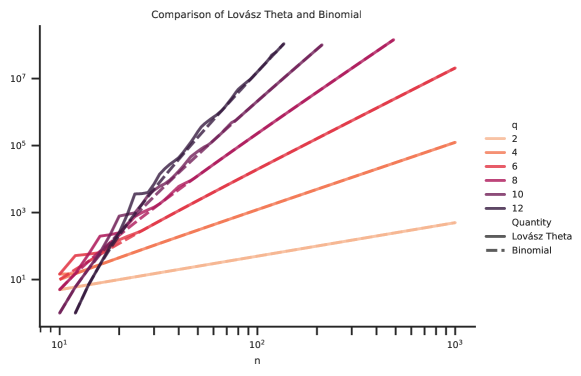
B.5 Numerics on Lovász theta function of local Majorana operators
In this section we present some numerics on the Lovász theta function of the commutation graph of degree- Majorana operators .
| 2 | 1 | 1 | ||||||||
| 4 | 2 | 1 | 2 | 1 | ||||||
| 6 | 3 | 3 | 1 | 3 | 3 | 1 | ||||
| 8 | 4 | 14 | 4 | 1 | 4 | 6 | 4 | 1 | ||
| 10 | 5 | 14.57 | 14.57 | 5 | 1 | 5 | 10 | 10 | 5 | 1 |
| 12 | 6 | 15 | 52 | 15 | 6 | 6 | 15 | 20 | 15 | 6 |
| 14 | 7 | 21 | 57.34 | 57.34 | 21 | 7 | 21 | 35 | 35 | 21 |
| 16 | 8 | 28 | 64 | 198 | 64 | 8 | 28 | 56 | 70 | 56 |
| 18 | 9 | 36 | 100.13 | 218.34 | 218.34 | 9 | 36 | 84 | 126 | 126 |
| 20 | 10 | 45 | 153.11 | 251.22 | 787.17 | 10 | 45 | 120 | 210 | 252 |
| 22 | 11 | 55 | 195.13 | 429.91 | 885.15 | 11 | 55 | 165 | 330 | 462 |
| 24 | 12 | 66 | 236.42 | 759 | 982.84 | 12 | 66 | 220 | 495 | 792 |
| 26 | 13 | 78 | 286 | 990.80 | 1757.0 | 13 | 78 | 286 | 715 | 1287 |
| 28 | 14 | 91 | 364 | 1217.2 | 3260.2 | 14 | 91 | 364 | 1001 | 2002 |
| 30 | 15 | 105 | 455 | 1444.2 | 4643.9 | 15 | 105 | 455 | 1365 | 3003 |
| 32 | 16 | 120 | 560 | 1820.0 | 6040.7 | 16 | 120 | 560 | 1820 | 4368 |
| 34 | 17 | 136 | 680 | 2423.3 | 7240.0 | 17 | 136 | 680 | 2380 | 6188 |
| 36 | 18 | 153 | 816 | 3327.1 | 9269.4 | 18 | 153 | 816 | 3060 | 8568 |
| 38 | 19 | 171 | 969 | 4512.8 | 12552 | 19 | 171 | 969 | 3876 | 11628 |
| 40 | 20 | 190 | 1140 | 6022.1 | 17230 | 20 | 190 | 1140 | 4845 | 15504 |
Appendix C Annealed approximation and concentration results
Consider the model
| (73) |
where are standard independent Gaussians and are deterministic matrices. The Gibbs state at inverse temperature is defined by
| (74) |
where is called the partition function at inverse temperature . The factor ensures that the free energy is extensive and scales proportionally to .
In this section we show that the commutation index of the terms has an important effect on the concentration properties of the random model . Denote the commutation index by
| (75) |
Recall that this quantity characterizes the variance of the energy with respect to a fixed state :
| (76) |
The value of has implications for relations between the normalized quenched and annealed free energies:
| (77) |
The quenched free energy is physical but hard to calculate while the annealed free energy is much easier to calculate but nonphysical. The first result is that this variance quantity controls the difference between the two.
Theorem C.1 (Quenched and annealed free energy).
| (78) |
Therefore, a small variance means that the annealed free energy well-approximates the quenched free energy, which indicates the absence of spin glass order [13]. The next three results give concentration of expectation values, energy, and two-point correlators of the thermal state of . Two-point correlators are of special interest in the study of the SYK model [13, 58, 68, 69]. Concentration results for Lipschitz bounded functions of the spectrum of the SYK model have also been established in [70].
Theorem C.2 (Concentration of expectation values).
For any fixed bounded operator ,
| (79) |
Theorem C.3 (Concentration of energy).
| (80) |
where .
Theorem C.4 (Concentration of two-point correlators).
For any fixed bounded operators and , denoting
| (81) |
for any , we have:
| (82) |
Instantiating for example Theorems C.1, C.2, C.3, C.4 with the upper bound on the commutation index of Majoranas in B.2 yields the following results for the SYK model.
Corollary C.1.
(SYK model is annealed.) For the SYK model where is even,
| (83) | |||
| (84) | |||
| (85) | |||
| (86) |
and are any fixed bounded operators.
Importantly, the above result shows that for the standard SYK model with , the quenched free energy in the limit of always equal its annealed approximation for physical temperatures where . This stands in stark contrast with spin glasses where a transition occurs for some critical temperature into a clustered or ‘glassy’ phase (see Appendix A).
The remainder of this appendix is concerned with establishing Theorems C.1, C.2, C.3, C.4 for concentration of various observables and free energies.
C.1 Preliminaries
Let us first state a useful fact about Lipschitz functions of Gaussian variables.
Fact C.1 (Gaussian concentration of Lipschitz functions, Theorem 2.26 of [71]).
Let be i.i.d. standard Gaussian variables, and -Lipschitz. Then for any :
| (87) |
Our first step is to establish concentration for the eigenvalues of using this fact.
Lemma C.1 (Concentration of eigenvalues).
For all and any eigenvalue of ,
| (88) |
Proof.
We apply C.1 to . It suffices to show has Lipschitz constant bounded by . Observe that for any fixed state ,
| (89) |
The function also has the same Lipschitz bound, as a result of the following argument. The eigenvalue in Hilbert space can be written in the min-max variational form:
| (90) |
The above statement guarantee that there exists subspaces and of dimension and respectively with non-zero intersection where for any and , it holds
| (91) |
For a given set of coefficients , let be the Hamiltonian of a different set of coefficients . Define subspaces and as before and let . Then
| (92) |
By symmetry, we similarly have . Thus and is -Lipschitz. C.1 completes the proof. ∎
In the course of proving our results we will also use an equivalent formulation of C.1 that follows from its sub-Gaussianity [72, 73, 74].
Lemma C.2 (Sub-Gaussian MGF bound, Lemma 1.5 of Ref. [72]).
Given a random variable with sub-Gaussian concentration bound
| (93) |
it holds that
| (94) |
C.2 Proof of C.1
C.3 Proof of C.2
The result once again follows from a Lipschitz bound. We use the well-known expression for the derivative of a matrix exponential [75]:
| (95) |
From the chain rule we then have:
| (96) |
Consider now the operator:
| (97) |
We can check that has trace norm bounded by . Denoting by the th singular value of in nonincreasing order, we have by the majorization inequality [76]:
| (98) |
that
| (99) |
This implies that has trace norm bounded by . However, is not necessarily positive semidefinite. We instead consider as the difference of two positive semidefinite matrices:
| (100) |
where each of is a (unnormalized) quantum state. By the cyclic property of the trace we can then write:
| (101) |
We thus have:
| (102) | ||||
| (103) | ||||
| (104) |
The result then follows from C.1.
C.4 Proof of C.3
We would like an analog of Eq. (101) where the observable is . Notice this is -dependent and commutes with . We get:
| (105) |
Let denote the ground energy of , and let be the set of coefficients where . For :
| (106) | ||||
| (107) | ||||
| (108) | ||||
| (109) |
C.5 Proof of C.4
Completely analogously to the proof of C.2 we have:
| (116) |
where:
| (117) |
We now focus on the final term of Eq. (116). We have:
| (118) |
where is the Hermitian, time-averaged operator:
| (119) |
We have:
| (120) | ||||
| (121) | ||||
| (122) |
To proceed, consider (for instance):
| (123) |
is Hermitian by definition and has trace norm bounded by by the matrix Hölder inequality (or alternatively, an analog of the singular value majorization argument used in the proof of C.2). Once again we can consider as the difference of two positive semidefinite matrices:
| (124) |
Doing this for all terms yields:
| (125) | ||||
| (126) | ||||
| (127) | ||||
| (128) |
Appendix D Lower bound on SYK optimum
Consider a Hamiltonian weighted by i.i.d. Gaussian coefficients
| (129) |
where we here assume that all . We show a lower bound for the maximal eigenvalue for such a Hamiltonian.
Theorem D.1 (Lower bound on the maximal eigenvalue).
There is an absolute constant such that
| (130) |
The commutation index is defined in B.1. We have also defined the commutation degree
| (131) |
and the global norm
| (132) |
Our results in the main text are only reported in the case all for simplicity. Note that here, both and feature a quadratic sum (instead of a linear sum) due to the randomness of the Hamiltonian.
This immediately gives lower bounds for the SYK maximal eigenvalue.
Corollary D.1.
With high probability over the disorder, the maximum eigenvalue of the SYK model is
| (133) |
Proof.
Our theorem also lower bounds the maximal eigenvalue of a -local quantum spin glass:
| (134) |
Corollary D.2.
With high probability over the disorder, the maximum eigenvalue of the -local quantum spin glass model is
| (135) |
when .
Proof.
The strategy to prove D.1 is to lower bound the optimum by calculating the exponential
| (Concentration for the maximal eigenvalue: C.1) | ||||
| (136) |
where we use to denote the normalized trace. We begin by lower bounding the right-hand side.
Lemma D.1 (Lower bounds on the exponential).
There is an absolute constant such that for each
| (137) |
In proving Lemma D.1 we will use the below two facts.
Fact D.1 (Integration by parts).
For standard Gaussian random variable and a function whose derivative is absolutely integrable w.r.t. the Gaussian measure, we have that
| (138) |
Fact D.2 (Multivariate Hölder for random matrices [37, Fact A.1]).
For any family of square random matrices, possibly statistically dependent, the product satisfies the trace inequality
| (139) |
where
| (140) |
Proof of Lemma D.1.
Take derivative w.r.t. :
| (141) | ||||
| (142) | ||||
| (Integration by parts: D.1) | ||||
| (Derivative of matrix exponential [75]) | ||||
| (143) |
The last line “swaps” the through the exponential, resulting in errors written as commutator, as seen from
| (144) |
and setting The intuition is that the commutator would be small due to the locality of . We further expand the second term
| (145) | |||
| (146) | |||
| (Integration by parts: D.1) |
Thus,
| (147) | |||
| (D.2 and ) | |||
| (148) | |||
| (By definitions of and ) |
The second inequality uses a multivariate Hölder’s inequality for random matrices (D.2), for moment parameters for each , and for each and Indeed, Also, the “” notation absorbs the absolute numerical constants arising from the insertions of and the integration over Thus, defining ,
| (149) | ||||
| (Gronwall’s differential inequality) | ||||
| (By the initial condition ) |
which concludes the proof. ∎
One immediate corollary of this lemma is the following, which follows from evaluating Eq. (137) at .
Corollary D.3 (A good ).
| (150) |
With the preliminaries in place we are now able to prove D.1. We will also use eigenvalue concentration bounds proved in Appendix C.
Appendix E Circuit lower bound for SYK model
In this section we show that low-energy states of random strongly interacting fermionic Hamiltonians have high circuit complexity. In particular, we show a circuit lower bound on the low energy states of the the SYK model. It was previously described in Eq. (1), but we repeat its definition here for convenience.
Definition E.1.
Let denote the set of degree- Majorana operators on fermionic modes. The model is a random ensemble of Hamiltonians defined by
| (153) |
Theorem E.1.
(SYK model low-energy states have high circuit complexity.) Let denote the set of unitaries generated by quantum circuits with at most gates each taken from a finite universal set of -local unitary gates. Fix an arbitrary initial state . With high probability, for any even , it holds that the minimum circuit complexity to construct a state achieving at least on is at least
| (154) |
Meanwhile, we can recall D.1 from Appendix D, which gives a lower bound on the maximum eigenvalue of SYK.
The proof of E.1 will proceed via a concentration argument, followed by a union bound over the circuit family. This resembles the circuit lower bound of [77, Appendix D]. We establish the necessary concentration now, which relies crucially on B.2 concerning the commutation index of low-degree Majorana operators.
Lemma E.1.
Fix any state . The energy sharply concentrates:
| (155) |
Proof.
Proof of E.1..
Let be the number of gates in the universal gate set. Then the number of circuits in is at most
| (158) |
Performing a union bound on E.1 yields
| (159) |
For this to be non-vanishing in , it requires
| (160) |
∎
Remark E.1.1.
The proof above can be extended to gates with continuous parameters by forming an -net over the gates. This comes at the cost of additional factors in the bound of E.1.
Remark E.1.2.
E.1 Relation to NLTS results
Our circuit lower bound is closely related to the study of ‘no low-energy trivial states’ (NLTS) Hamiltonians. Introduced in [51], a Hamiltonian has the NLTS property if there is no constant-depth circuit preparing a state whose energy is above the ground energy by less than some constant fraction of the norm . Such Hamiltonians were first proven to exist in [35] using quantum LDPC codes.
The circuit lower bounds we give are not quite comparable to the traditional notion of NLTS. This is because we compare the energy of our low-energy states to the Hamiltonian’s maximum eigenvalue rather than the norm of the coefficients. Unlike the quantum code Hamiltonian studied in [35, 36], the SYK model is highly frustrated and thus the operator norm and norms have vastly different scalings: and , respectively.
Despite these differences from the standard NLTS setting, the circuit lower bounds we can establish are much stronger in two ways when compared to current progress on NLTS [79, 80, 81, 36, 35]. First, our circuit lower bounds hold for states at any energy which is a constant fraction of the ground state energy, rather than for states below some constant-fraction energy threshold. Second, we can achieve arbitrary polynomial circuit depth lower bounds, whereas current constructions of NLTS only give a logarithmic depth lower bound.
E.2 Other Notions of Nontriviality
Though our focus so far has been on quantum circuit lower bounds, our results readily generalize to lower bounds for other classes of ansatzes via the construction of covering nets. We begin by discussing tensor networks, focusing on matrix product states (MPSs) as a particular example. Implemented at any finite precision the number of configurations of a matrix product state on sites grows with the bond dimension as . It is thus apparent from the same argument that the minimum bond dimension such that there is an MPS achieving an energy is
| (161) |
with high probability. Similarly, a classical neural network representation of the state with weights has a number of configurations growing as , yielding the growth condition to achieve an energy with high probability:
| (162) |
E.3 Product state approximations for spin Hamiltonians
It is worth pointing out that there cannot be a -local spin Hamiltonian with the property in E.1. For any traceless -local spin Hamiltonian , there is a product state achieving energy at least . The argument is imported from [24, proof of Theorem 2], and the proof technique bears a remarkable resemblence to the classical shadows protocol [82], which provides a learning algorithm for -local spin operators.
Theorem E.2.
For any -local Hamiltonian on qubits, there is a product state achieving energy
| (163) |
Proof.
Let be the true (possibly entangled) maximum-energy state achieving
| (164) |
For each qubit, pick a random basis out of , and measure in this basis. This gives a product state of single-qubit stabilizer states. Let be the resulting ensemble of pure product states we will analyze . It turns out that
| (165) |
where is the depolarizing channel
| (166) |
Thus
| (167) |
Here we used that is traceless and -local. ∎