Analytical planar wavefront reconstruction and error estimates
for radio detection of extensive air showers

Abstract

When performing radio detection of ultra-high energy astroparticles, the planar wavefront model is often used as a first step to evaluate the arrival direction of primary particles, by adjusting the wavefront orientation based on the peak of signal traces of individual antennas. The benefits of this approach are however limited by the lack of a good evaluation of its robustness.
In order to mitigate this limitation, we derive in this work an analytical solution for the arrival direction as well as the corresponding analytical reconstruction uncertainty.
Because it is fast and robust, this reconstruction method can be used as a proxy for more complex estimators, or implemented online for low-level triggering.

1 Introduction

An extensive air shower (EAS) is produced when a high-energy particle (cosmic ray, gamma ray, neutrino or one of its secondary particles) interacts with molecules of the atmosphere, generating a cascade of daughter particles. In air, this development can be used to detect the highest energy astroparticles for instance via the direct collection of the daughter particles, or the shower radiation production in Cherenkov, fluorescence light, or radio. For all these techniques, determining the arrival direction of the primary particle is key. First because it serves as a fundamental discrimination against terrestrial emissions. Second because it can be a useful ingredient to reconstruct the other parameters of the air-shower, such as its energy or the nature of the primary particle. The arrival direction can also be used to discern cosmic rays from neutrinos, mostly emerging from below the horizon. Finally, this has become crucial in the current multi-messenger astronomy era, for source identification and follow-up searches.

In this work, we focus on the radio-detection technique. The electromagnetic component of the shower undergoes charge separation due to the geomagnetic field and other less prominent processes. The resulting varying current leads to an emission in the radio regime, which can be detected by simple antennas arrays (see e.g., reviews by [1, 2]). This concept has been successfully tested with various experiments like LOPES [3], CODALEMA [4], LOFAR [5], AERA [6], TREND [7]. These instruments have focused on vertical showers, arriving with low inclination with respect to the zenith. The arrival direction can be reconstructed by making use of the timing information collected at each antenna in the array, and fitting a wavefront model, accounting for the varying light propagation speed in the atmosphere. A robust determination of the initial radiation emission direction thus requires a correct modeling of the wavefront.

The shape of the wavefront as observed on the ground depends strongly on the ratio between the emission region size and the distance to the detector. Vertical showers present rather close-by emission-point configurations: geometrically, one can infer that the wavefront curvature is quasi-spherical close to the shower axis, and becomes conical further out, leading to a hyperbolic function. The pioneering LOPES [8] and CODALEMA [4] experiments found that plane or hyperbolic wave modelings enabled indeed reasonable reconstructions. The efficiency of the hyperbolic modeling was further confirmed by LOFAR analysis [9]. On the other hand, showers arriving with very inclined zenith angles, as targeted by next-generation radio detectors like GRAND [10] or BEACON [11], imply that the observer is located at large distances from the emission region. Recent studies [12] have demonstrated that the wavefront shape could then be modeled more accurately by a spherical function.

Generally, the planar wavefront (PWF) model is found to be a reasonable first step to evaluate the arrival direction independently of any configuration. The simplicity of the planar wavefront modeling allows for a fast and analytical computation, which can be implemented online at first detector triggering levels. We present in this work a full analytical methodology to calculate the arrival direction using the planar wavefront model, and assess its robustness and efficiency. Most importantly, we precisely evaluate the errors associated to this computation. Such estimates are lacking in the literature: the source positions are reconstructed without associated, theoretically-motivated uncertainties. On the contrary, this study provides the community with both reliable direction reconstruction and uncertainty estimations. The source code implementing the methods described below is publicly available in [13].

The layout of this paper is as follows. In Section 2 we present our methodology, its formalism, the solutions and the error estimation calculations. In Section 3, we evaluate the performances of our method, and discuss the outcomes in Section 4.

2 Methodology

2.1 Problem formulation and solution

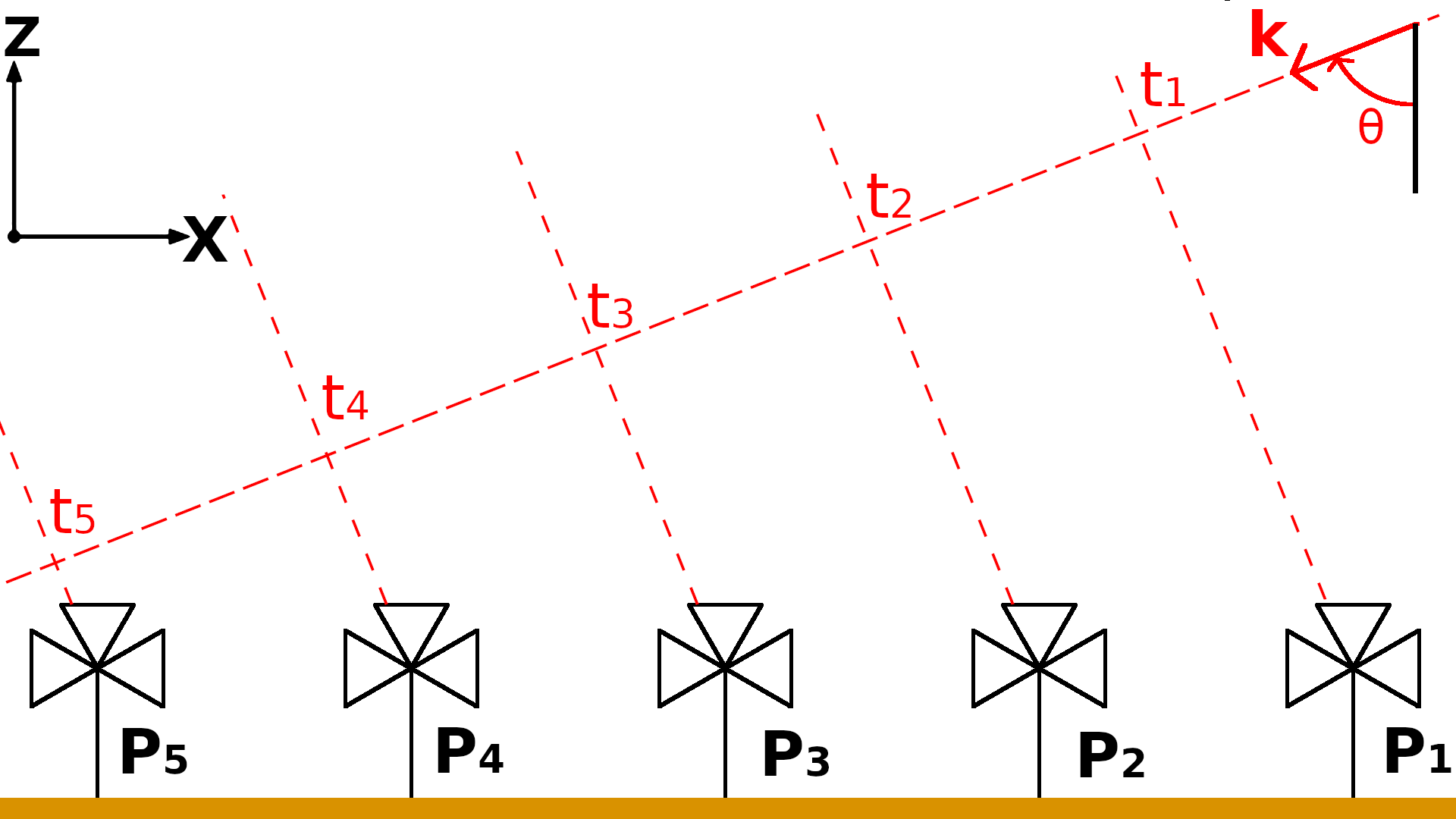
Figure 1: 2d representation of the planar wavefront model. The cosmic ray (coming from the right), generates a wave with a wavefront perpendicular to the direction of propagation. All antennas on a same perpendicular plane to the direction of propagation will be triggered at the same time.

Under the assumption that the wavefront is planar, as depicted on Fig. 1, the time of arrival on antenna $i$ can be related to the direction vector $\mathbf{k}$, the position of the antenna $\mathbf{p}_{i}$, and a time of reference $t_{0}$ as follows:

$$t_{i}=\frac{1}{c^{\prime}}\mathbf{p}_{i}\cdot\mathbf{k}+t_{0}\text{; }\ \mathbf{k}=\left(\begin{matrix}k_{x}\\ k_{y}\\ k_{z}\end{matrix}\right)\ ,$$ (1)

where $c^{\prime}$ is the average speed of light in the traversed medium. Here $\mathbf{k}$ is a unit vector as the signal must prop- agate at the speed of light. It is normal to the wavefront and in the direction of propagation of the signal. It directs the shower axis in the PWF case. With the angle convention used, we define the zenith angle $\theta$ and azimuth angle $\phi$ of the air shower by the following equation:

$$\mathbf{k}=\left(\begin{matrix}k_{x}\\ k_{y}\\ k_{z}\end{matrix}\right)\ =\left(\begin{matrix}-\sin(\theta)\cos(\phi)\\ -\sin(\theta)\sin(\phi)\\ -\cos(\theta)\end{matrix}\right)\ .$$ (2)

Equation 1 can be written in vector format, to account for $n$ antennas:

$$\mathbf{T}=\mathbf{P}\,\mathbf{k}+\mathbf{\epsilon}\ ,$$ (3)

with $\mathbf{\epsilon}$ the noise impinging each antenna: $\mathbf{\epsilon}\thicksim\mathcal{N}\left(\mathbf{0},\ \mathbf{Q}\right)$, with

$$\mathbf{Q}=\text{diag}(\sigma_{1}^{2},\sigma_{2}^{2},...,\sigma_{n}^{2})$$ (4)

with $\sigma_{i}$ the standard deviation of the noise on $t_{i}$. T is a length n vector encapsulating all timings : $\mathbf{T}=c^{\prime}[t_{i}-\bar{t}]_{i=\{1..n\}}$, and $\mathbf{P}=[\mathbf{p}_{i}-\bar{\mathbf{p}}]_{i=\{1..n\}}$ a $n\times 3$ matrix. $\bar{t}$ and $\bar{\mathbf{p}}$ are the weighed averages of the times and positions of the antennas:

$$\bar{\mathbf{p}} = \frac{1}{\sum_{i}{\sigma_{i}}^{-2}}\sum_{i}\frac{\mathbf{p}_{i}}{{\sigma_{i}}^{2}}$$ (5)

and

$$\bar{t} = \frac{1}{\sum_{i}{\sigma_{i}}^{-2}}\sum_{i}\frac{t_{i}}{{\sigma_{i}}^{2}}$$

In the rest of the paper, we will consider that all $\sigma_{i}$’s are equal to the same value $\sigma$. The weighted averages become simple averages. The rest of the calculations are unchanged.

Eq. 3 yields the following likelihood function :

$$\rm p(\mathbf{T}\,|\,\mathbf{P},\mathbf{k})=\frac{\exp{\left[-\frac{1}{2}(\mathbf{T}-\mathbf{P}\,\mathbf{k})^{T}\mathbf{Q}^{-1}(\mathbf{T}-\mathbf{P}\,\mathbf{k})\right]}}{{\left({2\pi\det{\mathbf{Q}}}\right)}^{n/2}}\ .$$ (6)

In order to estimate the direction of arrival $\mathbf{k}$, we need to find the maximum of the likelihood function, or equivalently, find the minimum of the negative log-likelihood function:

$$L_{\mathbf{P},\mathbf{T}}(k) =-\log\rm p(\mathbf{T}|\mathbf{P},\mathbf{k})$$

$$=\frac{1}{2}(\mathbf{T}-\mathbf{P}\mathbf{k})^{T}\mathbf{Q}^{-1}(\mathbf{T}-\mathbf{P}\mathbf{k})+A$$ (7)

under the constraint that

$$\|\mathbf{k}\|=1$$ (8)

Where $A$ is a constant that doesn’t interfere in the minimisation process. The solution to this process will be called $\mathbf{k_{MLE}}$.

We present two methods to solve this optimisation problem. The first one, a projection method, is only valid under the approximation that the antennas lie almost on the same plane but has the advantage of being fully analytical. The second method is a semi-analytical method and offers a more general solution.

2.1.1 Projection method

The minimum of the function in Eq. 7 without the constraint that $\|\mathbf{k}\|=1$ is given by:

$$\mathbf{k}^{*}=(\mathbf{P}^{T}\mathbf{Q}^{-1}\mathbf{P})^{-1}\mathbf{P}^{T}\mathbf{Q}^{-1}\mathbf{T}\ \ ,$$ (9)

as it is a linear regression problem.

Since the timing measurement errors are Gaussian, we can also express the distribution of $\mathbf{k}$ by:

$$\mathbf{k}\thicksim\mathcal{N}\left(\mathbf{k}^{\mathbf{*}},\ \mathbf{\Sigma}\right)\,,\text{ with }\mathbf{\Sigma}=(\mathbf{P}^{T}\mathbf{Q}^{-1}\mathbf{P})^{-1}\ .$$ (10)

This distribution is represented by the red contour lines in Figure 2. It is skewed along an axis close to the vertical line because the antennas lie almost on an horizontal plane. The component of $\mathbf{k}^{*}$ normal to this plane is reconstructed with low precision thus its covariance term is orders of magnitude higher than for the other components.

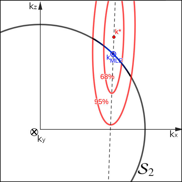
Figure 2: Visualisation of a cross section of the regression problem. The unconstrained linear regression produces $\mathbf{k}^{*}$ and the distribution represented by the red contour lines. The projection approximation projects $\mathbf{k}^{*}$ on the sphere along the dashed line (the large axis of the distribution). It is an approximation of $\mathbf{k_{MLE}}$, the maximum of likelihood on the unit sphere $\mathcal{S}_{2}$. The likelihood distribution under constraint is represented by the blue color gradient on the sphere. The distributions represented here are not to scale.

To apply the constraint, we disregard this component and set its value so that $\|\mathbf{k}\|=1$. On Fig. 2, it amounts to projecting $\mathbf{k}^{\mathbf{*}}$ along the dashed line onto the unit sphere $\mathcal{S_{2}}$. More formally, as $\mathbf{\Sigma}^{-1}$ is a positive-definite matrix, it can be diagonalised into an orthogonal basis: $\mathbf{\Sigma}^{-1}=\mathbf{\Phi}\mathbf{\Lambda}\mathbf{\Phi}^{T}$ with $\mathbf{\Lambda}$ a diagonal matrix composed of the eigen values of $\mathbf{\Sigma}^{-1}$ in decreasing order and $\mathbf{\Phi}$ an orthogonal transition matrix. The distribution given by Eq. 10 can then be written:

$$\rm p(\mathbf{k}) =C\exp\left[{-\frac{1}{2}\left(\mathbf{\Phi}^{T}\mathbf{k}-\mathbf{\Phi}^{T}\mathbf{k}^{*}\right)^{T}\mathbf{\Lambda}\,\left(\mathbf{\Phi}^{T}\mathbf{k}-\mathbf{\Phi}^{T}\mathbf{k}^{*}\right)}\right]$$ (11)

$$\text{ with: }\bm{\Lambda}=\left(\begin{matrix}\lambda_{1}&0&0\\ 0&\lambda_{2}&0\\ 0&0&\lambda_{3}\end{matrix}\right)$$

The eigen values $\lambda_{1}$, $\lambda_{2}$, $\lambda_{3}$ are such that: $\lambda_{3}\ll\lambda_{1},\lambda_{2}$.

Projecting $\mathbf{\Phi}^{T}\mathbf{k}^{\mathbf{*}}$ onto the unit sphere and along the eigen vector associated with $\lambda_{3}$ gives the final prediction in the eigen basis coordinates system. Projecting the resulting vector in the original $(\mathbf{x},\mathbf{y},\mathbf{z})$ coordinate system by multiplying by $\mathbf{\Phi}$ produces $\mathbf{k_{proj}}$ which is an approximation of the maximum likelihood estimator.

If $\mathbf{\Phi}^{T}\mathbf{k}^{*}=\left[k_{x^{\prime}},k_{y^{\prime}},k_{z^{\prime}}\right]^{T}$ then

$$\mathbf{k_{proj}}=\mathbf{\Phi}\left[k_{x^{\prime}},\ k_{y^{\prime}},\ -\sqrt{1-(k_{x^{\prime}}^{2}+k_{y^{\prime}}^{2})}\right]^{T}\ .$$ (12)

In the case where $k_{x^{\prime}}^{2}+k_{y^{\prime}}^{2}>1$, we set $k_{z^{\prime}}=0$ then normalise $\mathbf{\Phi}^{T}\mathbf{k}^{*}$ so that $k_{x^{\prime}}^{2}+k_{y^{\prime}}^{2}=1$. The negative sign before the square root favors negative values for $k_{z}$ as we expect down going EAS.

2.1.2 Semi analytical method

Eq. 7 is a quadratic form that is convex in $\mathbf{k}$ but the constraint that $\mathbf{k}$ lies on the unit sphere makes the optimization problem non-convex. However, the unit sphere is compact and the quadratic form is continuous, so we know that the optimization problem has a global minimum. For the sake of simplicity, let us look at the following problem:

$$\mathbf{k_{MLE}}=\operatorname*{arg\,min}_{\mathbf{k}}\mathbf{k}^{T}\mathbf{A}\mathbf{k}-2\mathbf{b}^{T}\mathbf{k},\quad s.t.\quad\|\mathbf{k}\|=1$$ (13)

with $\mathbf{A}$ positive semi-definite. In our case, by developing Eq. 7, we have:

$$\begin{cases}\mathbf{A}=\mathbf{\Sigma}^{-1}=\mathbf{P}^{T}\mathbf{Q}^{-1}\mathbf{P}\\ \mathbf{b}=\mathbf{P}^{T}\mathbf{Q}^{-1}\mathbf{T}\\ \end{cases}$$ (14)

It can be shown [14] that $\mathbf{k}$ is a solution of Eq. 13 if and only if there exist $\mu$ such that $\mathbf{A}+\mu\mathbf{I}$ is positive semidefinite, and $(\mathbf{A}+\mu\mathbf{I})\mathbf{k}=\mathbf{b}$.

Let us diagonalise the matrix, $\mathbf{A}=\mathbf{\Phi\Lambda\Phi}^{T}$ like in the previous subsection, where $\Lambda$ is the diagonal matrix whose diagonal are the eigen values $[\lambda_{1},\lambda_{2},\lambda_{3}]$ of $\mathbf{A}$ in decreasing order, and define $\bm{\beta}=\mathbf{\Phi}^{T}\mathbf{b}$.

The solution to Eq. 13 is given by $\mathbf{k_{MLE}}=\mathbf{\Phi}^{T}\mathbf{c}$ where $\mathbf{c}$ is computed in the following way: let us define $\mathcal{E}_{3}=\{i\mid\lambda_{i}=\lambda_{3}\}$ and $\mathcal{E}_{+}=\{i\mid\lambda_{i}>\lambda_{3}\}$. We then have two distinct cases:

• Degenerate case. If $\beta_{i}=0$ for all $i\in\mathcal{E}_{3}$, and

  $$\sum_{\mathcal{E}_{+}}\frac{\beta_{i}^{2}}{(\lambda_{i}-\lambda_{3})^{2}}\leq 1,$$ (15)

  then $\mu=-\lambda_{3}$ and $c_{i}=\beta_{i}/(\lambda_{i}-\lambda_{3})$ for all $i\in\mathcal{E}_{+}$. The values of $c_{i}$ for $i\in\mathcal{E}_{3}$ are chosen arbitrarily, as long as they ensure that $\mathbf{k}$ is of unit norm: $\sum_{\mathcal{E}_{3}}c_{i}^{2}=1-\sum_{\mathcal{E}_{+}}c_{i}^{2}$.

• Non degenerate case. In this case, we have $c_{i}={\beta_{i}}/{(\lambda_{i}+\mu)}$, such that $\sum c_{i}(\mu)^{2}=1$. The function on the left hand side of the last equation is strictly convex in $\mu$, in the interval $[-\lambda_{3}+\sqrt{\sum_{\mathcal{E}_{3}}b_{i}^{2}},-\lambda_{i}+\|b\|]$ . $\mu$ can then be estimated with a line search algorithm.

Once $\mathbf{c}$ is obtained, we can multitply by $\mathbf{\Phi}$ to get $\mathbf{k_{MLE}}$. The degenerate case corresponds to when the antennas lie on a common plane, the solution is the same as the approximate solution from the previous subsection.

For all previous methods, a final step is added to ensure the reconstructed $\mathbf{k}$ points downward. When the predicted vector points upward, we reflect it through the plane formed by the antennas, whose normal vector is the eigen vector associated with $\lambda_{3}$.

2.2 Uncertainty

The classical linear regression with no constraint produces the distribution of $\mathbf{k}$ given $\mathbf{P}$ and $\mathbf{T}$ : $\rm p(\mathbf{k}|\,\mathbf{P},\mathbf{T})$ as shown in Eq. 10.

Applying the constraint amounts to looking for:

$$\rm p(\mathbf{k}|\,\mathbf{P},\mathbf{T},\|\mathbf{k}\|=1)$$ (16)

rather than $\rm p(\mathbf{k}|\,\mathbf{P},\mathbf{T})$. As we show in Sect. 3, the reconstruction errors of the estimators proposed in the previous section are small (typically less than a degree). We can assume that the unit sphere is locally flat and approximated by its tangent plane at $\mathbf{k_{MLE}}$, $\mathcal{T}_{\mathbf{MLE}}$. The distribution of $\mathbf{k}$ on the unit sphere is thus locally approximated by the distribution on $\mathcal{T}_{\mathbf{MLE}}$.

$$\rm p\left(\ \mathbf{k}\ |\,\mathbf{P},\mathbf{T},\,\|\mathbf{k}\|=1\right)\approx\rm p\left(\ \mathbf{k}\ |\,\mathbf{P},\mathbf{T},\,\mathbf{k}\in\mathcal{T}_{\mathbf{MLE}}\right).$$ (17)

We will write the previous vectors in the basis $\mathbf{b}=(\mathbf{\hat{e_{r}}},\mathbf{\hat{e_{\theta}}},\sin\rm\theta\ \mathbf{\hat{e_{\phi}}})$, the spherical basis associated with $\mathbf{k_{MLE}}$ scaled by $\sin\theta$ along $\mathbf{\hat{e_{\phi}}}$. We will add a subscript $\rm sph$ to vectors expressed in this basis.

let us denote by $\mathbf{R}$ the transition matrix:

$$\mathbf{k_{sph,MLE}}=\mathbf{R}\,\mathbf{k_{MLE}}=\left(\begin{matrix}1\\ 0\\ 0\end{matrix}\right)\ .$$ (18)

The basis $\mathbf{b}$ is such that the tangent plane $\mathcal{T}_{\mathbf{MLE}}=\left\{\mathbf{k_{sph}}\in\mathbb{R}^{3}\mathbf{|}\ \mathbf{k_{sph}}\cdot\mathbf{\hat{e_{r}}}=1\right\}$ and that $(\mathbf{\hat{e_{\theta}}},\sin\rm\theta\ \mathbf{\hat{e_{\phi}}})$ is a basis of $\mathcal{T}_{\mathbf{MLE}}$. Furthermore, for small variation $\mathbf{dk_{sph}}$ close to $\mathbf{k_{sph,MLE}}$ on $\mathcal{T}_{\mathbf{MLE}}$ we have:

$$\mathbf{dk_{sph}}=\left(\begin{matrix}0\\ \rm d\theta\\ \rm d\phi\end{matrix}\right)+\,o(\mathbf{dk_{sph}})=\left(\begin{matrix}0\\ \mathbf{k_{a}}\end{matrix}\right)+\,o(\mathbf{dk_{sph}}),$$ (19)

where $\rm d\theta$ and $\rm d\phi$ are small variations of zenith and azimuth angles.

Rewriting 10 in this new basis gives:

$$\mathbf{k_{sph}}\thicksim\mathcal{N}\left(\mathbf{k_{sph}}^{\mathbf{*}},\ \mathbf{R}\mathbf{\Sigma}\mathbf{R}^{T}\right)\ .$$ (20)

Let $\mathbf{k_{a}}\in\mathbb{R}^{2\times 1}$ and $k_{r}\in\mathbb{R}$ such that $\mathbf{k_{sph}}=[k_{r},\,\mathbf{k_{a}}^{T}]^{T}$. Let $\mathbf{k_{a}}^{\mathbf{*}}\in\mathbb{R}^{2\times 1}$ and $k_{r}^{*}\in\mathbb{R}$ such that $\mathbf{k_{sph}}^{\mathbf{*}}=[k_{r}^{*},\,{\mathbf{k_{a}}^{\mathbf{*}}}^{T}]^{T}$. Finally, let $\mathbf{\Sigma_{rr}}\in\mathbb{R}$, $\mathbf{\Sigma_{aa}}\in\mathbb{R}^{2\times 2}$ and $\mathbf{\Sigma_{ar}}\in\mathbb{R}^{2\times 1}$. such that:

$$\mathbf{R}\mathbf{\Sigma}\mathbf{R}^{T}=\left(\begin{matrix}\mathbf{\Sigma_{rr}}&\mathbf{\Sigma_{ar}}^{T}\\ \mathbf{\Sigma_{ar}}&\mathbf{\Sigma_{aa}}\end{matrix}\right)\ .$$ (21)

Each of these quantities are denoted by $\mathbf{r}$ if they involve the coordinate along $\mathbf{\hat{e_{r}}}$ and by $\mathbf{a}$ if they involve a coordinate corresponding to an angle (along $\mathbf{\hat{e_{\theta}}}$ or $\sin\rm\theta\ \mathbf{\hat{e_{\phi}}}$). For example, $\mathbf{\Sigma_{rr}}$ is the variance of the distribution along $\mathbf{\hat{e_{r}}}$.

The condition "$\mathbf{k}\in\mathcal{T}_{\mathbf{MLE}}$" translates into "$k_{\rm r}=1$". The conditional distribution is Gaussian with covariance matrix:

$$\bar{\bm{\Sigma}} = \rm{Cov}(\mathbf{k_{a}}\,|\,k_{\rm r}=1)=\rm{Cov}\left(\left(\begin{matrix}\theta\\ \phi\end{matrix}\right)\right)$$ (22)

$$= \mathbf{\Sigma_{aa}}-\frac{1}{\mathbf{\Sigma_{rr}}}\mathbf{\Sigma_{ar}}^{T}\mathbf{\Sigma_{ar}}$$

To summarize, the final distribution of the reconstructed zenith and azimuth is given by:

$$\left(\begin{matrix}\theta\\ \phi\end{matrix}\right)\thicksim\mathcal{N}\left(\left(\begin{matrix}\theta_{\rm MLE}\\ \phi_{\rm MLE}\end{matrix}\right),\,\bar{\mathbf{\Sigma}}\right),$$ (23)

where $\theta_{\rm MLE}$ and $\phi_{\rm MLE}$ are the zenith and azimuth angles of $\mathbf{k_{MLE}}$.

The expression for $\bar{\mathbf{\Sigma}}$ in Eq. 22 is the Schur complement of the block matrix $\mathbf{R}\mathbf{\Sigma}\mathbf{R}^{T}$. Its inverse is the corresponding block in the block matrix $\left(\mathbf{R}\mathbf{\Sigma}\mathbf{R}^{T}\right)^{-1}$. We thus have:

$$\bar{\mathbf{\Sigma}}=\left[\mathbf{R_{a}}^{T}\mathbf{\Sigma}^{-1}\mathbf{R_{a}}\right]^{-1}$$ (24)

with

$$\mathbf{R_{a}}=\left(\begin{matrix}-\cos(\theta)\cos(\phi)&\sin(\theta)\sin(\phi)\\ -\cos(\theta)\sin(\phi)&-\sin(\theta)\cos(\phi)\\ \sin(\theta)&0\\ \end{matrix}\right).$$ (25)

In practice, we approximate $\mathbf{R_{a}}$ by replacing $\theta$ by $\theta_{\rm{MLE}}$ and $\phi$ by $\phi_{\rm{MLE}}$, the zenith and azimuth angles of $\mathbf{k_{MLE}}$.

If we denote by $\psi$ the angle between the prediction $\mathbf{k_{MLE}}$ and the target direction $\mathbf{k}$:

$$\psi=\cos^{-1}(\mathbf{k}\,\cdot\,\mathbf{k_{MLE}}).$$ (26)

We can estimate the mean value of $\psi^{2}$ as

$$\|\mathbf{k_{MLE}}-\mathbf{k}\|^{2}=\psi^{2}+o(\psi^{3})$$ (27)

thus

$$<\psi^{2}>\approx<\|\mathbf{k_{MLE}}-\mathbf{k}\|^{2}>\approx\rm tr(\mathbf{C}\bar{\mathbf{\Sigma}}\mathbf{C})$$ (28)

with

$$\mathbf{C}=\left(\begin{matrix}1&0\\ 0&\sin(\theta_{\rm MLE})\end{matrix}\right).$$

This correspond to the uncertainty described in [15]:

$$<\psi^{2}>=\sigma_{\theta\theta}^{2}+\sin^{2}{(\theta)}\,\sigma_{\phi\phi}^{2}$$ (29)

with $\sigma_{\theta\theta}$ and $\sigma_{\phi\phi}$, the diagonal values of $\bar{\mathbf{\Sigma}}$, which correspond to the variance of the estimators of $\theta$ and $\phi$.

3 Performances

To evaluate the performances of the direction estimators as well as the uncertainty estimator, we will use two distinct sets of simulations.

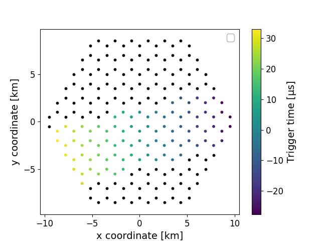
Figure 3: Antenna layout. Antennas are placed on an hexagonal grid with 1000 m side length. Every event only triggers a subset of all the available antennas. Here, the layout intersected a cosmic ray with a zenith angle $\theta=87.1$°, azimuth $\phi=14.5$° and energy $E=4.0$ EeV. The triggered antennas are color-coded according to the arrival times.

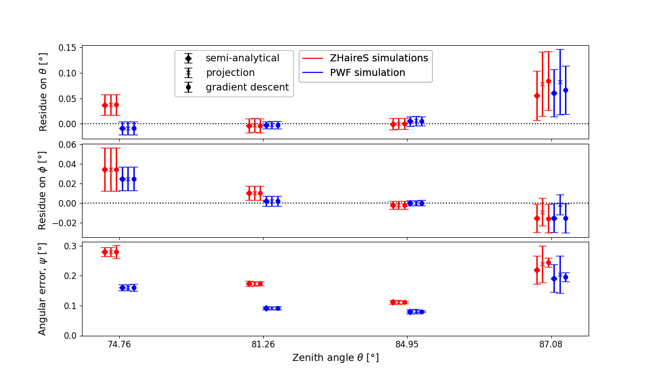
Figure 4: Mean zenith (top) and azimuth (middle) angle reconstruction residus on the PWF and ZHAireS simulation esets. The bottom plot represents the mean angular error, defined in Eq. 26 The error bars represent one standard deviation of the mean value estimator.

• We first use a set of 1500 ZHAireS simulations [16] sampled at selected antenna locations (see Fig. 3). We use the same simulation procedure as the one described in [17]. These are simulation of the electric field sampled every 0.5ns. They have been generated with a discrete number of input parameters:

  • 5 values of zenith angle $\theta$ : [63.01°, 74.76°, 81.26°, 84.95°, 87.08°]. After applying the trigger criterion, no events are left with $\theta=63.01$°

  • 5 values of energy $E$ : [0.1, 0.3, 0.63, 1.6, 4.0] EeV

  • 3 types of primary type : [proton, gamma, iron]

  • Azimuth angle $\phi$ randomly sampled between 0° and 180°

  To make data closer to antenna measurements, we do a series of transformation to the data. First, we filter the traces to keep only frequencies between 50 MHz and 200 MHz with a band-pass filter. We extract the maximum amplitude and time of maximum of the Hilbert envelope of the resulting traces. Antennas with signal amplitude lower than $90\,\rm{\mu}$V/m are disregarded as it would not trigger the trace recording, according to typical noise levels. Furthermore, any EAS that triggered less than 5 antennas according to previous trigger criterion are rejected. After these quality cuts, we are left with 555 simulated events. We then add a Gaussian noise with a standard deviation of 10 ns to the timings to represent the noise introduced by the GPS and measurements uncertainties. This new set of simulation let us assess the performances on data as close as possible to what a radio antenna would measure from a EAS.

  This dataset will be referred as the ZHAireS simulation set in the following sections.

• We also consider a second set of simulations based on the planar wavefront modelling. From every event of the ZHAireS simulation set, we create a corresponding one with the same triggered antennas. The sole difference is that we replace the wavefront arrival times by times generated by a planar wavefront with the same zenith and azimuth angles. Similarly as the ZHAireS set, we add a Gaussian noise with a standard deviation of 10 ns.

  This second simulation set is useful to show the performance of the methods in an idealised situation where the only errors come from the stochasticity of the data and the solver approximations but not from a discrepancy between the simulation and the model used to reconstruct the arrival direction. In addition, it let us generate many realisations of the same event but with different noise values. We will refer to this set of simulations as the PWF simulation set.

3.1 Estimator precision

In this section, we compare the two methods defined in section 2 with the more established and traditionally used gradient descent type techniques that are usually considered in this type of analysis [12, 15].

For each simulation set, we apply the projection, semi-analytical and gradient descent estimators to the simulated arrival times, and present the binned residues in the top and middle panels of Fig. 4. For a proper reconstruction we use a fixed refractive index $n_{\rm{atm}}=1.00014$ (see  A for more details).

As can be seen, the two new methods presented in this work give similar and consistent results (diamond and cross symbols) compared to the gradient descent (dot symbol). It should be noted that all the methods also provide residues consistent with zero, meaning that they do not exhibit significant bias on both simulation sets. While this is expected for the PWF simulation set, which is generated using the same model as the estimators, the fact that this is also the case for the ZHAireS set demonstrates the the PWF formalism, despite its simplicity is a very good descriptions of very inclined EAS.

On the bottom panel of Fig. 4, we present the mean angular errors for the three estimators and two simulation sets. This is the mean value of the angle $\psi$ as described in section 2. This error is always positive and describe the pointing precision of the estimator. On average, the angular error is around 0.2° for all zenith angles.

3.2 Uncertainty calibration

In this section, we investigate the calibration of the theoretical uncertainties that we computed in Sect. 2 and verify their calibration. Essentially, uncertainties are well calibrated when the reported variance, e.g. if we assume a Gaussian distribution, matches the empiric variance, which is determined by considering the dispersion of the results of the estimator. We illustrate this on Fig. 5 where we compare the theoretical uncertainties from Eq 24 to the dispersion of reconstructed events for the PWF simulation set. More specifically, we considered one specific event from the PWF simulation set (this event has $\theta=81.26$°, and $\phi=7.69$°), and generated 10000 different timing noise realizations, resulting in 10000 different events coming form the same direction. We applied the semi-analytical estimator to each of these events, and show the 2-d histogram of the reconstructed events in blue on Fig. 5. We also show the 1-d histogram along each angle coordinate. We show in red the 68%, 95%, and 99.5% theoretical contours, derived from Eq. 24, as well as the 1-d probability function on top of the 1-d blue histogram. As can be seen, both the empirical and theoretical distributions are consistent.

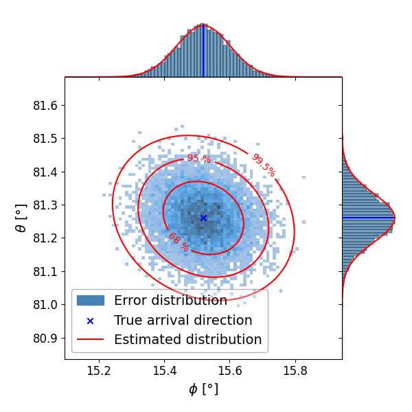
Figure 5: Example of confidence regions prediction, the uncertainty estimation closely matches the error distribution. The blue distribution is the histogram of many reconstruction of the same event ($\theta=81.26$°, $\phi=7.69$°) with different noise realisations. The red lines are the isolines of the estimated uncertainties.

We now turn our attention to the calibration on the ZHAireS simulation set. On Fig. 6 we show, for each zenith bin, the histogram of the differences between the arrival times in the raw ZHAireS simulations (before filtering and noise) and the one we would obtain with a planar wavefront. These histograms illustrate the fact that the wavefront simulated by ZHAireS isn’t perfectly planar, they represent the deviation of the simulated wavefront from an idealised planar wavefront. For each zenith bin, we add the variance of these time differences, denoted $\sigma_{\rm model}^{2}$, to the Gaussian timing noise variance, resulting in adding an effective systematic Gaussian noise to the previous noise distribution:

$$\sigma_{\rm{tot}}^{2}=\sigma_{\rm model}^{2}+\sigma^{2}\ .$$ (30)

More generally, we can measure the calibration of uncertainties with a prediction interval coverage probability (PICP) diagram. For a chosen percentage, say $68\%$, we measure on our dataset the proportion of events where the true arrival direction lie inside the $68\%$ confidence region given by the theoretical uncertainties. If those are correctly calibrated, we expect this proportion to be close to $68\%$. We represent this diagram on Fig. 7 for the PWF (triangles) and ZHAireS (cross) simulation sets for 68%, 95% and 99.5% intervals. The envelop represents the statistical deviation tolerated (2 standard deviation) inside which we can consider that we are well calibrated. If the value is outside this envelop, we can confidently say the estimator isn’t perfectly calibrated. It is the case for zenith around $82$° but the PICP metric lies most of the time in the acceptable range around its target value.

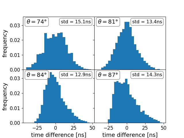
Figure 6: Histogram of the difference of arrival times between the ZHAireS and PWF simulation set for the four zenith bins that are considered.

3.3 Computational efficiency

Finally, we compare the computation efficiency of the different methods. The PWF reconstruction method described in [15] and [18] use an alternative loss function:

$$L^{\prime}_{\mathbf{P},\mathbf{T}}(k) = \sum_{i,j}{\left((t_{i}-t_{j})-\frac{1}{c^{\prime}}(\mathbf{p}_{i}-\mathbf{p}_{j})\cdot\mathbf{k}\right)^{2}}$$ (31)

$$= \|\mathbf{\Delta T}-\mathbf{\Delta P}\mathbf{k}\|^{2}$$

This loss function is mathematically equivalent to Eq. 7 but has a time complexity of $\mathcal{O}(n^{2})$ while Eq. 7 is in $\mathcal{O}(n)$ making it computationally faster. The minimisation of this loss function with gradient descent with respect to $\theta$ and $\phi$ is calling the function $d$ times so the total complexity of commonly used method is $\mathcal{O}(dn^{2})$. Conversely, the time complexity of the analytical-solutions or projection approximation is the time complexity of the linear regression or $\mathcal{O}(3^{2}n+3^{3})=\mathcal{O}(n)$ (3 because we work in 3 dimension). The time complexity of inverting $\mathbf{Q}$ is linear as $\mathbf{Q}$ is a diagonal matrix. Furthermore, the complexity of finding $\mu$ in the semi-analytical method has very small impact on the performances.

The analytical estimators have much less computation to do, especially for large footprints and could therefore be used in an inline configuration for direct reconstruction.

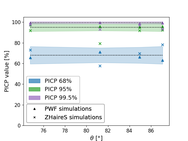
Figure 7: Prediction Interval Coverage Probability (PICP) for 68%, 95% and 99.5% quantiles on PWF dataset (triangle) and ZHAireS dataset (cross). The uncertainty estimator is well calibrated on PWF dataset but under-confident around 82° on the ZHAireS simulations. The shaded region are 95% confidence intervals of the PICP estimator (2 standard deviations).

4 Conclusions, discussion

We have proposed a mathematical and probabilistic approach to the planar wavefront description of air showers. By construction, the direction of propagation of the wavefront is linearly dependent on the time of arrival and the positions of the antennas. We have demonstrated that despite the constraint that the propagation vector must be unitary, an analytical solution exists. A geometrical approach allows us to estimate the uncertainty on the reconstruction from the uncertainty on the measurements. The analytical uncertainty estimation for reconstruction also allows for the prediction of error bars and confidence regions for direction estimators that are reliable for a wide range of zenith angles. This reconstruction method can be fast and robust and used as a proxy for more complex estimators as well as an online reconstruction method for triggering procedure or first direction estimation.

Appendix A Refraction index refinement

To model the wavefront, a proper description of the wave propagation speed is necessary. This speed depends on the medium traversed by the signal. If the EAS starts to develop high in the atmosphere, the mean refractive index would be smaller than for a EAS that starts closer to the ground where the atmosphere density is larger. Given an event, the mean refractive index is different for every antenna.

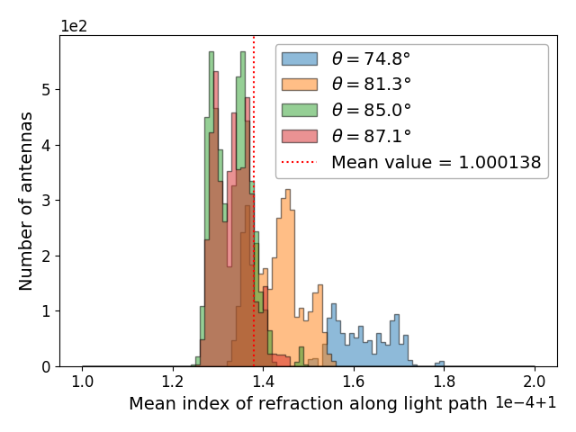
Figure 8: Distributions of mean refractive indices for all events and all antennas in the ZHAireS simulation set. The refractive index calculated is the mean index between $X_{\rm max}$ position, a proxy of the virtual source position, and the antenna position.

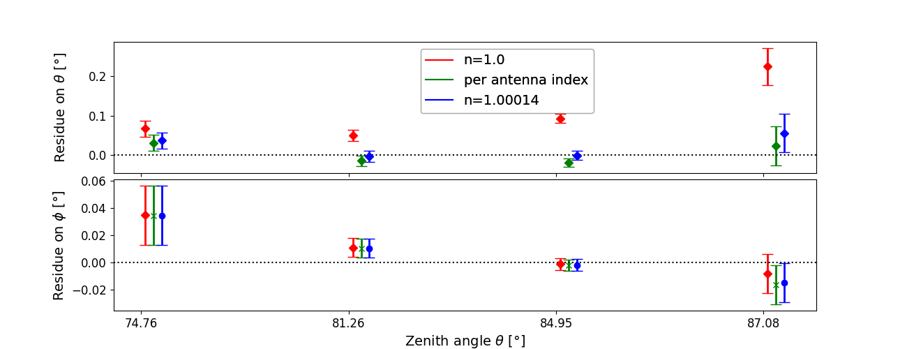
Figure 9: Mean zenith (top) and azimuth (bottom) angle reconstruction residues on ZHAireS simulation set using a refractive index $n_{\rm{atm}}=1$ (red), $n_{\rm{atm}}=1.00014$ (blue), and a refractive index varying for every antenna (green).

To compute this refractive index along the light path, we consider that the signal travels in a straight line and was emitted at the location of $X_{\rm max}$ [12]. The effective refractive index model used is the same as the one in the ZHAireS simulations [16]. We represent on Fig. 8 the histograms of the mean refractive indices along the light path for every event and every antenna in the ZHAireS simulation set.

We present in Fig. 9 the binned residues for $\theta$ and $\phi$ reconstruction o the ZHAireS simulation set using the semi-analytical method, where we consider a refractive index $n_{\rm{atm}}=1$ (red), $n_{\rm{atm}}=1.00014$ (blue), and a refractive index varying for every antenna (green). As can be seen, it is necessary to account for the atmosphere density. However using an average value for all the events and antennas provides satisfactory results, and alleviates the need to recompute the refractive index for every antenna.

References

-
[1]
T. Huege, Radio
detection of cosmic ray air showers in the digital era, Physics Reports 620
(2016) 1–52.
doi:10.1016/j.physrep.2016.02.001.
URL https://doi.org/10.1016%2Fj.physrep.2016.02.001 -
[2]
F. G. Schröder, Radio
detection of cosmic-ray air showers and high-energy neutrinos, Progress in
Particle and Nuclear Physics 93 (2017) 1–68.
doi:10.1016/j.ppnp.2016.12.002.
URL https://doi.org/10.1016%2Fj.ppnp.2016.12.002 -
[3]
H. Falcke, et al., Detection and
imaging of atmospheric radio flashes from cosmic ray air showers, Nature
435 (7040) (2005) 313–316.
doi:10.1038/nature03614.
URL http://dx.doi.org/10.1038/nature03614 -
[4]
D. Ardouin, et al.,
Radio-detection signature
of high-energy cosmic rays by the codalema experiment, Nuclear Instruments
and Methods in Physics Research Section A: Accelerators, Spectrometers,
Detectors and Associated Equipment 555 (1–2) (2005) 148–163.
doi:10.1016/j.nima.2005.08.096.
URL http://dx.doi.org/10.1016/j.nima.2005.08.096 -
[5]
M. P. van Haarlem, et al.,
Lofar: The low-frequency
array, Astronomy & Astrophysics 556 (2013) A2.
doi:10.1051/0004-6361/201220873.
URL http://dx.doi.org/10.1051/0004-6361/201220873 -
[6]
T. Huege, Radio detection
of cosmic rays with the auger engineering radio array, EPJ Web of
Conferences 210 (2019) 05011.
doi:10.1051/epjconf/201921005011.
URL http://dx.doi.org/10.1051/epjconf/201921005011 -
[7]
D. Charrier, et al.,
Autonomous radio
detection of air showers with the trend50 antenna array, Astroparticle
Physics 110 (2019) 15–29.
doi:10.1016/j.astropartphys.2019.03.002.
URL http://dx.doi.org/10.1016/j.astropartphys.2019.03.002 -
[8]
W. Apel, et al., The
wavefront of the radio signal emitted by cosmic ray air showers, Journal of
Cosmology and Astroparticle Physics 2014 (09) (2014) 025–025.
doi:10.1088/1475-7516/2014/09/025.
URL http://dx.doi.org/10.1088/1475-7516/2014/09/025 -
[9]
A. Corstanje, et al.,