Casting Light on Degeneracies: A Comprehensive Study of Lightcurve Variations in Microlensing Events OGLE-2017-BLG-0103 and OGLE-2017-BLG-0192
Abstract
This study investigates orbital parallax in gravitational microlensing events, focusing on OGLE-2017-BLG-0103 and OGLE-2017-BLG-0192. For events with timescales 60 days, a Jerk Parallax degeneracy arises due to high Jerk velocity (), causing a four-fold continuous parallax degeneracy. OGLE-2017-BLG-0103, after incorporating orbital parallax, reveals four discrete degenerate parallax solutions, while OGLE-2017-BLG-0192 exhibits four discrete solutions without degeneracy. The asymmetric light curve of OGLE-2017-BLG-0103 suggests a more probable model where xallarap is added to the parallax model, introducing tension. The galactic model analysis predicts a very low mass stellar lens for OGLE-2017-BLG-0192. For OGLE-2017-BLG-0103, degenerate solutions suggest a low-mass star or a darker lens in the disc, while the Xallarap+Parallax model also predicts a stellar lens in the bulge, with the source being a solar-type star orbited by a dwarf star. This study presents five degenerate solutions for OGLE-2017-BLG-0103, emphasizing the potential for confirmation through high-resolution Adaptive Optics (AO) observations with Extremely Large Telescopes in the future. The complexities of degenerate scenarios in these microlensing events underscore the need to analyze special single-lens events in the Roman Telescope Era.
1 Introduction
Gravitational microlensing (Einstein, 1936; Paczynski, 1986) is an intriguing astronomical phenomenon where the gravity of a foreground lens causes the light from a background source to bend, resulting in the appearance of multiple images when their relative proximity in the sky is closer than the which is given by,
| (1) |
where 4G/ 8.14 , is the mass of the lens, and and are the distances to the lens and source, respectively. These images are not individually resolved, distinguishing microlensing from . Instead, microlensing is detectable as a temporary fluctuation in the brightness of the source star when continuously observed over days or months. This phenomenon produces a characteristic light curve known as the Paczyǹski Curve (Paczynski, 1986) when plotted over time. It was only through the establishment of dedicated survey groups such as OGLE-I (Udalski et al., 1994), EROS (Aubourg et al., 1994), and MACHO (Bennett et al., 1993), that the first microlensing event toward the galactic bulge was observed (Alcock et al., 1995a, b). Since then, this field has rapidly expanded, shedding light on the mysteries of the inner Milky Way, thanks to the latest generation of survey telescopes like OGLE-IV (Udalski et al., 2015), KMTNet (Kim et al., 2016) and MOA-III (Bond et al., 2001; Sumi et al., 2003) equipped with a wide-field camera.
A straightforward way to parameterize a microlensing event is to consider a point lens, a point source, and the observer-lens-source combination moving in relative motion. In such a scenario, the separation between the lens and the source, normalized to the angular Einstein radius of the lens, is given by:
| (2) |
Here, is a function of time , and represent the impact parameters and the time of the closest approach, and corresponds to the time the source takes to cross the Einstein Radius. The time-varying magnification is then given by:
| (3) |
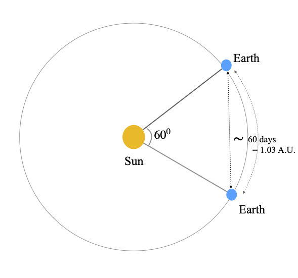
Although the lens itself cannot be directly detected during a microlensing event, higher-order effects can sometimes be observed, leading to the characterization of the lens. One such effect is known as Microlensing Parallax (), which is a vector quantity having a magnitude equal to and a direction similar to the project lens-source proper motion () (Equation (4)). Orbital parallax causes the source to follow a non-rectilinear trajectory, resulting in an asymmetric light curve, which becomes significant for events lasting 60 days or longer (Gould et al., 1994; Alcock et al., 1995a; Mao et al., 2002; Soszyński et al., 2001; Bond et al., 2002; Bennett et al., 2002b, a; Smith, 2003). During this period, the Earth’s displacement around the Sun is approximately 1.03 A.U. (see Figure (1)). The typical value of for M-dwarf lenses towards the bulge is around 2 A.U., which, while larger, is comparable to the chord length depicted in Figure 1. For events with shorter timescales (), the chord length is much smaller than 1.03 A.U., rendering unconstrained due to negligible perturbations in the light curve. However, for longer-duration events where the displacement exceeds the chord length, can be effectively constrained, resulting in a noticeably asymmetric light curve. Alternatively, even if the timescale of an event is larger than 60 days, but the lens has a low mass, then the value of will be smaller, and hence the won’t be constrained properly eventually leading to degenerate solutions.
| (4) |
Note that the is a vector quantity and the direction of the vector is similar to the direction of the lens-source proper motion ( = /) vector (Gould, 1992). Then, the mass of the lens can be calculated using,
| (5) |
where is the relative lens-source parallax. So, the mass of the lens can be measured if we know the value of or in addition to . Since the lens is usually faint and distant, we cannot measure (and hence ) directly. The parameter is also obtained from the lightcurve when finite-source effects are measured (see Gould (1994); Witt & Mao (1995); Nemiroff & Wickramasinghe (1994)). Interestingly, only a handful of single-lens events have
directly measured the value of either by measuring finite-source effects in extremely high magnification events (Yoo et al., 2004; Gould et al., 2009), via resolution of microlensing images using interferometry (Delplancke et al., 2001; Dong et al., 2019), or via astrometric-microlensing (Hog et al., 1995; Sahu et al., 2022). As these measurements are not possible for every microlensing event, measuring signatures in the lightcurve helps to put constraints on and .
For microlensing events having timescales 60 days, Gould (2004) showed that they suffer from a four-fold continuous degeneracy called as Jerk Parallax () degeneracy. This degeneracy is important when the value of is high and is 60 days. As increases, the continuous degeneracy is broken into discrete degeneracy and completely broken for very long events. We encourage the readers to refer Smith et al. (2003); Gould (2004) to understand the origins and fundamentals of this degeneracy. While this degeneracy has been explored before by Gould (2004); Jiang et al. (2004); Park et al. (2004); Poindexter et al. (2005), exactly, how does this degeneracy break as increases, and how do multi-site observations help in realizing this degeneracy has never been seen before. While the events analyzed by the first three authors had timescales 60 days, the latter found degenerate solutions in events having higher than 60 days.
In this paper, we present our analysis of the microlensing events OGLE-2017-BLG-0103 and OGLE-2017-BLG-0192. By modeling the light curve involving , we identify the existence of a discrete Jerk-Parallax degeneracy in the light curve of the former event but not later. We also explore the possibility of the source having an orbiting companion causing effects (also called xallarap) similar to the observed orbital parallax effect. For OGLE-2017-BLG-0103, we find a strong degeneracy between the orbital parallax and the Xallarap+Parallax model. We do not find such tension in OGLE-2017-BLG-0192.
1.1 Overview
After an introduction, we discuss the details of the data used in this analysis (2). In the initial part of Section (3), we describe the microlensing model that we fit the observed data followed by sub-Sections (3.1) and (3.2), where we talk about our approach to finding the Jerk-Parallax degenerate solutions (both giving similar results), followed by Section (3.3) where we discuss our Xallarap model. In Section (4), we analyze the source and the blend, followed by Section (5), where we obtain the distance to and mass of the lens. Finally, we discuss our results and conclude in Section (6).
2 Observations and Data Reductions
OGLE-2017-BLG-0103 is the 103rd event detected by the Early Warning System (EWS) of OGLE in the field BLG501.11 while OGLE-2017-BLG-0192 is the 192nd detected in the OGLE field BLG518.09. It was observed towards the galactic bulge through its 1.3m Warsaw Telescope, located at the Las Campanas Observatory in Chile Udalski et al. (2015). OGLE has a wide-field CCD camera, a mosaic of 32 2k x 4k individual chips. Together, they contribute to the camera having a wide FoV of 1.4 sq. deg. The calibrated source in both these events is a faint star with a baseline magnitude of 18.5 mag on the OGLE photometric maps. The equatorial co-ordinates of OGLE-2017-BLG-0103 are , which can be translated to galactic co-ordinates as , . Similarly, the equatorial coordinates for OGLE-2017-BLG-0192 are , , which can be translated to = (). We download the OGLE photometry for both events, which is available on its homepage. This photometry is generated after performing the difference image analysis of the field images that use the algorithm by Alard & Lupton (1998). Both these microlensing events were also observed independently by KMTNet through its three 1.8m telescopes spread across longitude in the southern hemisphere in Chile (KMT-C), South Africa (KMT-S), and Australia (KMT-A). Both these events were also found during the 2016 season by KMTNet’s event finder algorithm (Kim et al., 2018) and were designated in the KMTNet database as KMT-2017-BLG-1698 and KMT-2017-BLG-1225. All three KMTNet telescopes have wide-field cameras, each with four 9k x 9k chips to monitor the galactic field Kim et al. (2016). While OGLE-2017-BLG-0103 was observed in two fields - BLG02 and BLG42, OGLE-2017-BLG-0192 was observed in the field BLG31 by the KMTNet. Most of the observations were taken in the I band; there are occasional V band observations for these events. The KMTNet images in the I and V bands were reduced using the pyDIA software Albrow (2017), based on difference image analysis using the delta-basis-function approach of Bramich et al. (2013).
3 Analysis
As mentioned in the introduction, a single lens and single source lightcurve is described by three Pac̀zynski parameters: , , and . Two additional fit parameters, the and , are the source and blend fluxes obtained by performing a linear fit of the model to the observed data (refer Equation (6)). However, as we describe later, we incorporate a few additional parameters and form a higher-order model to fit the asymmetry in the data. We model the observed light curve of both events using the I band data of OGLE and KMTNet. So we have fourteen and eight values of and for OGLE-2017-BLG-0103 and OGLE-2017-BLG-0192, respectively, in addition to three Paczyǹski parameters to fit the observed light curve.
| (6) |
3.1 Orbital Parallax Model
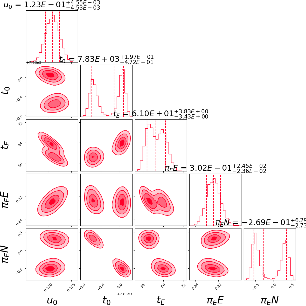
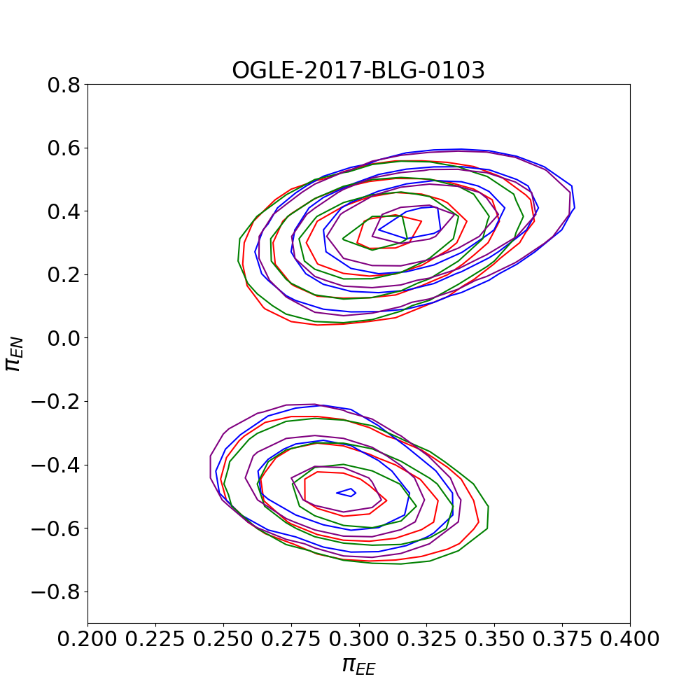
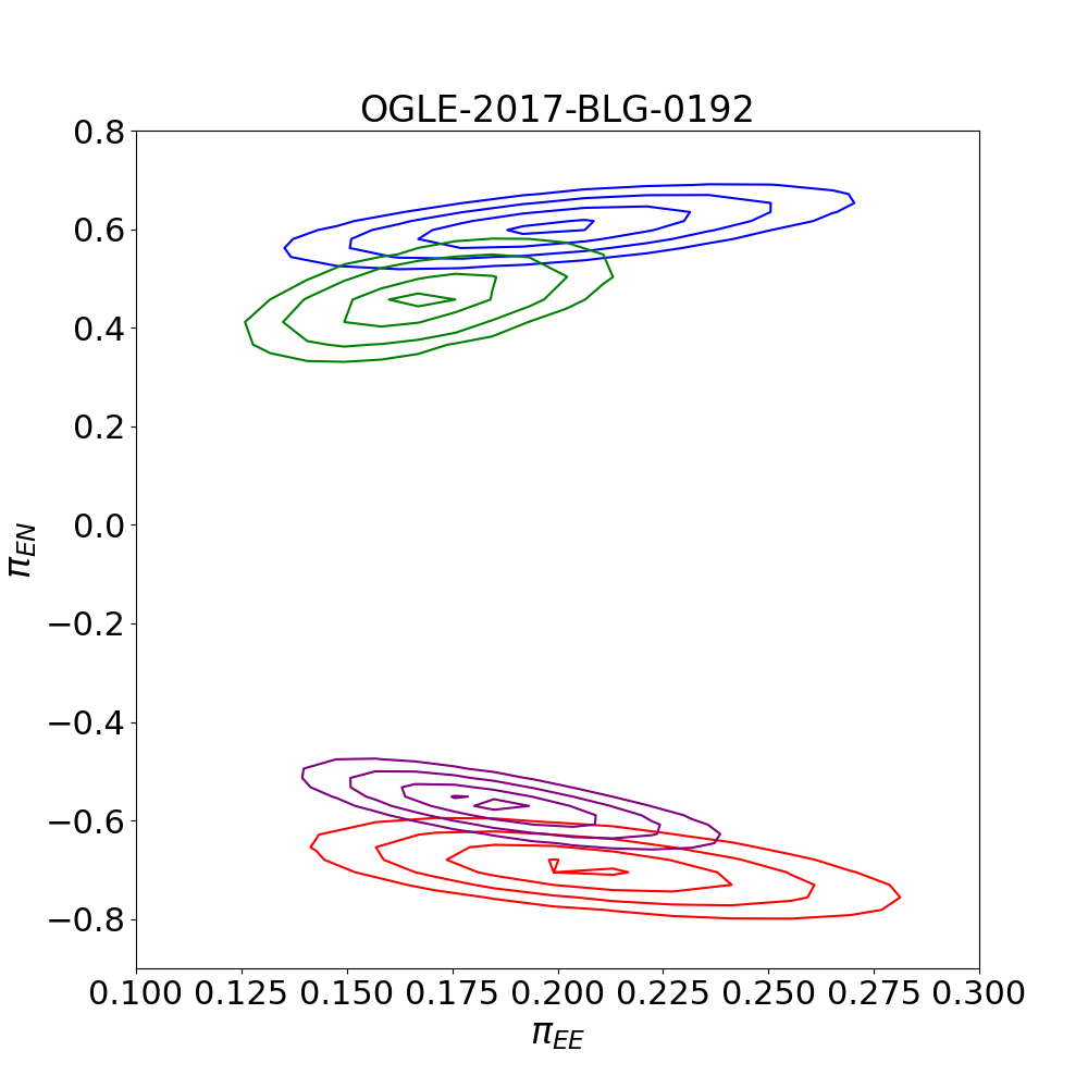
The single lens model did not fit the rising side of the asymmetric light curves of these events. So, we explore the orbital parallax model by adding two parameters and . We initially perform a coarse grid search minimizing in the (, ) plane by holding the Paczyński parameters constant. For OGLE-2017-BLG-0103, we found a minima at () = (0.184, -0.168) and for OGLE-2017-BLG-0192 at (0.120, -0.392) respectively. We seed these parameters along with Paczyński parameters to (Foreman-Mackey et al., 2013) and obtained a fitting model called P1. We then re-normalized the photometric uncertainties in magnitudes using the P1 model so that 1. After re-normalizing the photometric uncertainties, the P1 model was re-run, which converged to a solution shown in Figure (2a) where we see the Jerk-parallax degeneracy in the discrete contours of the model parameters. Similarly, Figure (2b) shows the P1 model parameter distributions for OGLE-2017-BLG-0192 where we do not see any bimodal distributions of , and parameters which indicate that the degeneracy is broken in this case.
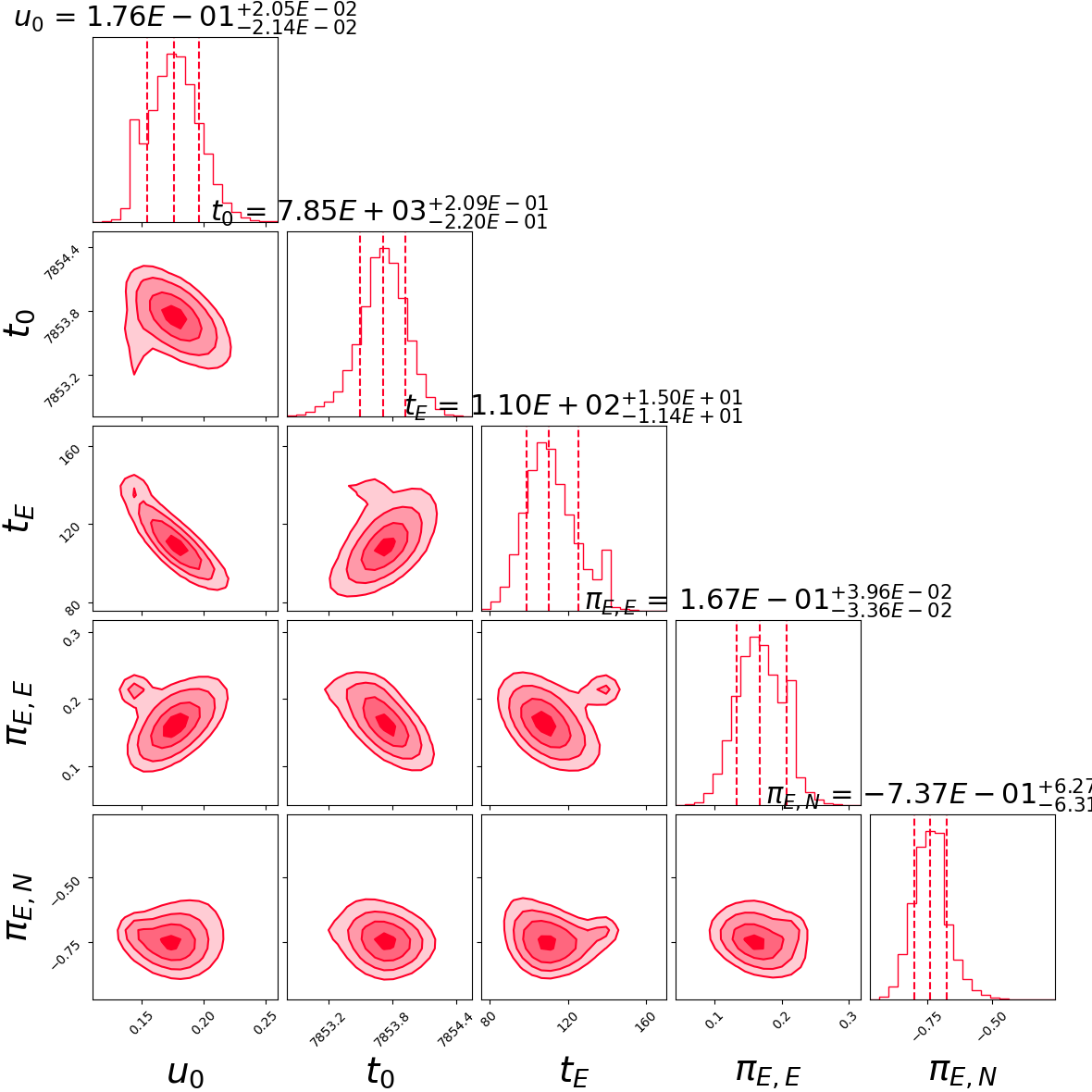
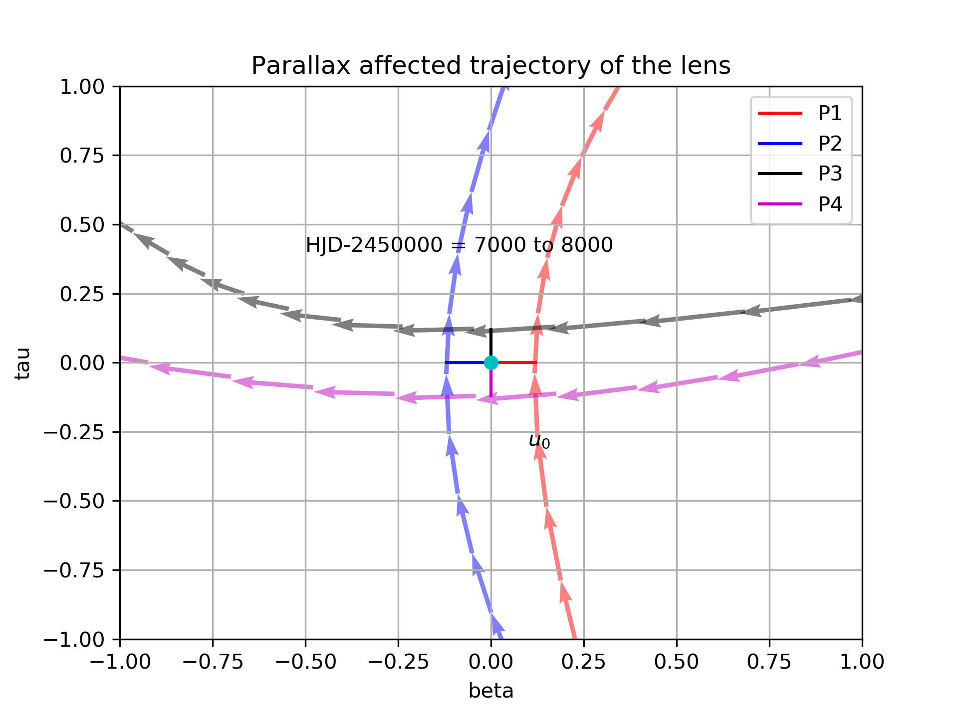
For OGLE-2017-BLG-0103, we term the model corresponding to the left mode in the distribution as P3. To explore the mirrored degenerate solutions, which are also the ecliptic degenerate solutions, we seed the emcee with the P1 model but with the sign of reversed (see Jiang et al. (2004); Poindexter et al. (2005), Skowron et al. (2011)). The walkers then converge to new solutions P2 and P4. Thus, we find all four degenerate solutions where P3 and P4 are the Jerk-Parallax degenerate solutions corresponding to P1 and P2, respectively. While P4 is the constant acceleration degenerate pair of P3, it is the ecliptic degenerate counterpart of P1 (and similarly, P2 is the constant-acceleration pair of P1 and ecliptic degenerate P3). The trajectories for these pairs take the path shown in Figure (3a). So, we must expect similar lens properties for each pair of ecliptic degenerate solutions but different for the Jerk-Parallax degenerate solution. In Figure (3b), we show the contours of of all the solutions. Although we do not see any bimodal distributions in the case of OGLE-2017-BLG-0192, we still repeat the above procedure and find that the discrete solutions are not very far from each other in the plane (see Figure (4b)).
3.2 Alternative method to find jerk parallax solutions
We show an alternative way to find the Jerk-Parallax degenerate solutions for the event OGLE-2017-BLG-0103 based on the framework by An et al. (2002); Smith et al. (2003); Gould (2004) and also used by Jiang et al. (2004) and Park et al. (2004). In this method, we find the Sun’s celestial position at the event’s peak and obtain the velocity () and acceleration (). At the time of the vernal equinox of the year 2017 (which was close to of OGLE-2017-BLG-0103), the acceleration of the Sun projected into the sky was
The projected acceleration points north through east in the sky. Since the parallax contours are elongated in the direction perpendicular to this direction at , to find the model P3, we first find and , the components of parallel and perpendicular to the acceleration of the Sun in the sky at (0.43, 0.00). Then, the perpendicular component of the degenerate parallax solution is found by using the relation:
| (7) |
where is the perpendicular component of the Jerk-Parallax and is calculated by,
| (8) |
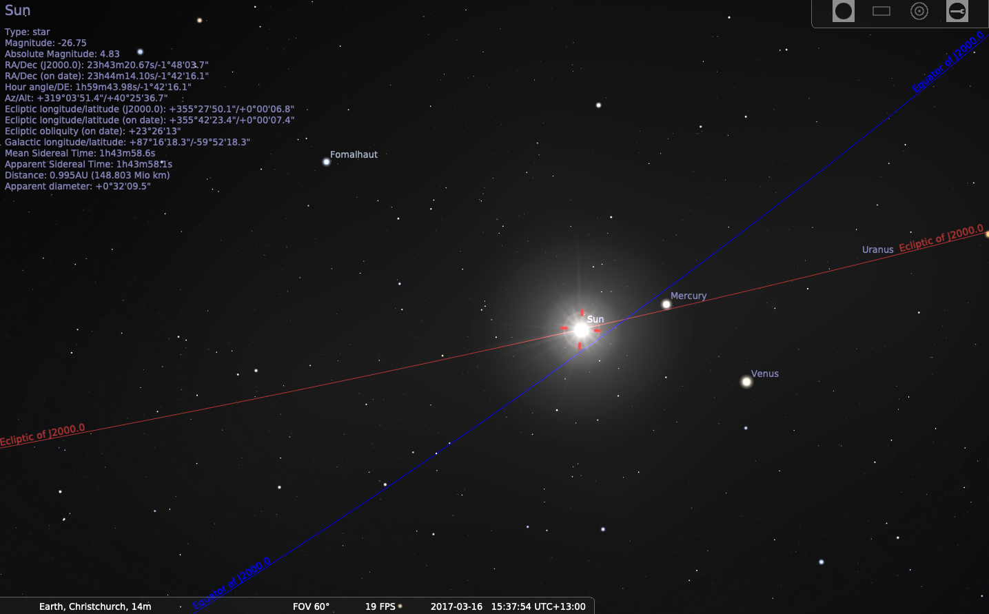
where is the ecliptic latitude of the event and is the phase of the Earth’s orbit. Using Equation (8), we get = 0.17. Thus, the location of the degenerate parallax solution is: () = (0.43, -0.17). The Sun’s path in the plane of the sky can be visualized in Figure (3b) where the background image is a screenshot of Stellarium v.0.15.1111www.stellarium.org and the ecliptic and equatorial planes are shown in red and blue colors, respectively. We can also see the projected position of the Sun close to the vernal equinox, the direction of projected acceleration towards the intersection of the ecliptic and equatorial planes. There is one component of parallel to the acceleration along the ecliptic and two anti-parallel perpendicular components causing this degeneracy.
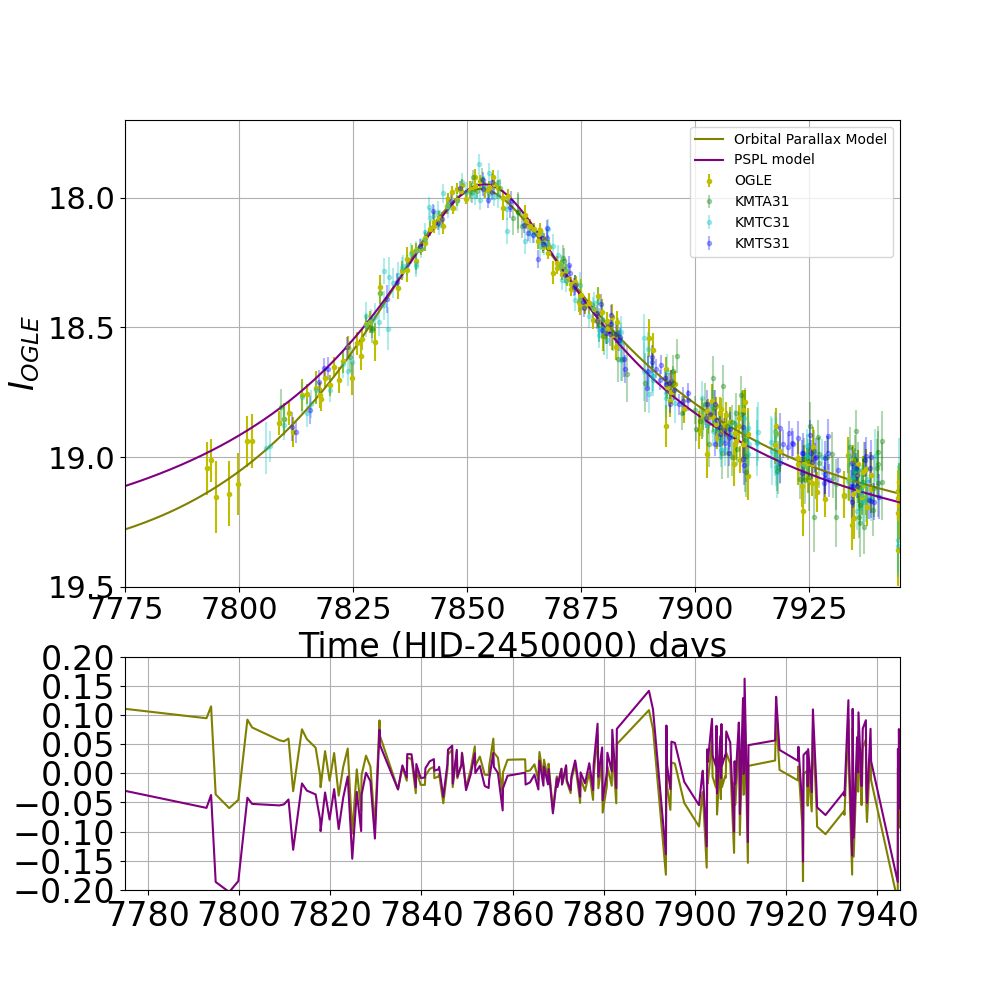
In Figure (4a), we see that the major axes of the elliptical co-variances in the first plot for OGLE are nearly perpendicular to each other. Since the direction of is the direction of in the adopted frame of reference, therefore, the direction of for P3 will be perpendicular to the direction of in P1 solution (see Figure (3a). As the direction of for P1 solution is arctan(/) = , the direction of for P3 solution should be . Thus, we can convert (,) derived earlier to celestial frame () = (0.30, -0.34) using (An et al., 2002). After seeding emcee with the Paczyński parameters of the P1 solution and these parallax parameters, we found that the median value of the degenerate parallax parameters is () = (0.30,-0.50). Furthermore, and also converge to the other mode of the bimodal distribution of the samples. Similarly, the other P4 solution was found using the P2 solution. In all the solutions, it is observed that 222 is responsible for the asymmetry about the base in the lightcurve. In contrast, is responsible for the asymmetry about the peak of the lightcurve. which is also seen in the light curve. The samples of the model parameters corresponding to each solution with their , , and percentile values are shown in Table (1). Similarly, the model parameters for the different parallax solutions with their , and percentile values for OGLE-2017-BLG-0192 are shown in Table (2) and the light curve in Figure (5).
| Microlensing model results | |||||||
|---|---|---|---|---|---|---|---|
| Parameter | PSPL | P1 | P2 | P3 | P4 | Xallarap | Xallarap + Parallax |
| 49123.42 | 11288.62 | 11290.50 | 11289.86 | 11290.90 | 11282.85 | 11237.26 | |
| 0.099 0.001 | 0.123 0.001 | -0.122 0.001 | 0.123 0.001 | -0.123 0.001 | 0.104 0.09 | ||
| (days) | 7829.90 0.01 | 7829.44 0.09 | 7829.67 0.03 | 7830.05 0.06 | 7829.67 0.03 | 7829.66 0.06 | 7830.37 0.04 |
| (days) | 73.12 0.01 | 58.26 1.62 | 60.42 2.12 | 63.91 2.22 | 60.23 2.06 | 73.17 3.22 | 53.632.07 |
| - | 0.31 0.02 | 0.30 0.02 | 0.30 0.02 | 0.30 0.02 | - | -0.014 0.004 | |
| - | 0.32 0.08 | -0.02 0.41 | -0.50 0.11 | 0.02 0.40 | - | 0.002 0.002 | |
| - | - | - | - | - | -0.001 0.002 | 0.001 0.001 | |
| - | - | - | - | - | 4.28 1.22 | ||
| - | - | - | - | - | 0.004 0.001 | 0.024 0.02 | |
| - | - | - | - | - | 1.56 0.02 | 1.56 0.01 | |
| - | - | - | - | - | 1.42 0.14 | 1.74 0.19 | |
| - | - | - | - | - | 0.0 | ||
| 2135.62 7.45 | 2142.26 8.57 | 2142.10 8.57 | 2139.82 3.21 | 2159.93 8.64 | 2140.78 9.32 | 2140.78 9.32 | |
| 1565.32 9.80 | 1570.63 11.40 | 1571.00 11.41 | 1568.81 5.49 | 1584.84 11.51 | 1570.67 11.12 | 1570.67 11.12 | |
| 2275.56 4.26 | 2323.37 4.53 | 2323.60 4.53 | 2321.11 7.97 | 2343.57 9.12 | 2321.25 4.62 | 2321.25 4.62 | |
| 2127.67 7.38 | 2125.29 7.37 | 2125.41 7.37 | 2123.11 7.37 | 2143.57 7.44 | 2124.68 7.03 | 2124.68 7.03 | |
| 1570.51 6.97 | 1578.11 7.98 | 1578.17 7.98 | 1575.87 4.52 | 1591.36 8.04 | 1576.63 7.99 | 1576.63 7.99 | |
| 2342.34 4.57 | 2323.30 5.49 | 2323.09 5.49 | 2320.80 11.39 | 2342.46 5.54 | 2322.00 5.30 | 2322.00 5.30 | |
| 2126.89 5.67 | 2125.77 5.84 | 2125.38 5.84 | 2123.36 8.56 | 2143.01 5.89 | 2126.87 6.32 | 2126.87 6.32 | |
| 1801.27 21.88 | 1803.28 22.81 | 1810.18 22.83 | 1811.93 22.80 | 1800.28 22.84 | 1801.21 22.43 | 1563.44 72.43 | |
| 2749.22 11.20 | 2747.28 11.43 | 2750.22 18.63 | 2752.91 11.43 | 2740.65 11.51 | 2745.24 12.21 | 2495.24 180.21 | |
| 2212.63 18.97 | 2213.61 19.18 | 2219.03 9.12 | 2221.69 19.18 | 2205.86 4.57 | 2745.24 12.21 | 1833.24 128.21 | |
| 12200.56 16.03 | 12177.35 15.99 | 12182.79 16.01 | 12185.16 15.99 | 12171.50 19.22 | 12177.73 16.78 | 11848.73 316.78 | |
| 2735.54 9.30 | 2738.75 9.10 | 2743.07 19.21 | 2745.75 9.10 | 2735.71 8.04 | 2736.98 9.12 | 2519.98 179.12 | |
| 2176.66 15.98 | 2177.66 18.60 | 2184.12 13.92 | 2186.66 18.60 | 2174.00 5.54 | 2176.76 17.76 | 1816.76 127.76 | |
| 12175.72 24.30 | 12172.96 22.80 | 12180.16 22.83 | 12181.64 22.80 | 12170.82 22.84 | 12175.96 25.40 | 11859.96 325.40 | |
| Microlensing model results | ||||||
|---|---|---|---|---|---|---|
| Parameter | PSPL | P1 | P2 | P3 | P4 | Xallarap |
| 4810.66 | 1540.73 | 1548.62 | 1581.93 | 1568.16 | 1636.83 | |
| 0.134 0.005 | 0.14 0.02 | -0.10 0.02 | 0.08 0.02 | -0.11 0.02 | ||
| (days) | 7853.78 0.06 | 7853.69 0.19 | 7853.33 0.19 | 7850.52 0.39 | 7851.31 0.29 | 7830.120.25 |
| (days) | 122.70 0.06 | 139.97 22.16 | 196.42 41.39 | 175.93 30.66 | 137.01 21.00 | |
| - | 0.21 0.03 | 0.20 0.03 | 0.17 0.02 | 0.19 0.02 | - | |
| - | -0.70 0.05 | 0.61 0.04 | 0.46 0.04 | -0.57 0.04 | - | |
| - | - | - | - | - | 0.0002 0.0001 | |
| - | - | - | - | - | ||
| - | - | - | - | - | 0.0048 0.0008 | |
| i | - | - | - | - | - | 1.571 0.001 |
| - | - | - | - | - | ||
| - | - | - | - | - | ||
| 1373.28 5.88 | 1374.07 6.00 | 1371.29 6.01 | 1372.89 6.00 | 1373.28 6.02 | 2949.99 14.70 | |
| 19738.09 311.20 | 19737.93 316.31 | 19732.00 318.63 | 19735.91 312.43 | 19735.65 311.51 | 35827.25 150.20 | |
| 11618.32 102.97 | 11615.34 102.09 | 11609.99 103.12 | 11612.32 103.18 | 11612.86 102.57 | 21038.56 198.67 | |
| 23098.56 191.52 | 23099.35 190.98 | 23104.18 196.01 | 23085.16 195.99 | 23071.50 193.22 | 42085.30 22.08 | |
| 1308.62 12.45 | 1308.13 12.37 | 1306.06 8.57 | 1306.53 6.21 | 1309.65 7.64 | -284.13 7.89 | |
| 15652.32 653.80 | 15648.00 653.16 | 15711.00 614.41 | 15648.81 648.49 | 15804.84 611.51 | 126.39 4.56 | |
| 13201.72 294.26 | 13156.13 293.72 | 13178.62 288.58 | 13165.11 297.97 | 13149.57 290.12 | 4229.28 38.32 | |
| 18078.63 460.59 | 18077.67 467.27 | 18069.81 480.01 | 18075.00 477.37 | 18070.00 467.44 | 159.63 7.79 | |
3.3 Xallarap effect
Like the motion of the Earth around the Sun, a companion orbiting to the source might also cause similar perturbations in the light curve due to orbital parallax (Griest & Hu, 1992; Paczynski, 1997; Dominik, 1998; Smith et al., 2003). When the orbital effect is insignificant, the light curve of a binary-source event can be assumed as the superposition of the lightcurves of static individual sources. Conversely, in cases where the orbital effect is substantial, it necessitates the incorporation of the orbital dynamics. The study of binary sources and their orbital motion in microlensing lightcurves may even provide new opportunities: it may help break degeneracies in microlensing (Griest & Hu, 1992; Han & Gould, 1997; Paczynski, 1997), or it may open a new channel to discover planets orbiting around the source star (Rahvar & Dominik, 2009; Bagheri et al., 2019; Miyazaki et al., 2021). The periods of binary systems may range from a few hours for very close systems to hundreds of years for widely spaced pairs. But binary source microlensing is not sensitive to long-period orbital signatures in the lightcurve (Rahvar & Dominik, 2009). Also, given the steepness of the luminosity-mass relation, in most cases, the secondary star might be much fainter than the primary. Consequently, though we might not detect flux from the companion in such cases, the companion may still be able to modulate its trajectory on the lens plane. For this reason, the binarity of the source may sometimes arise just from the perturbation of the motion of the host without any signs of additional light, and the light curve can be similar to that of the orbital parallax modulated light curve. We, therefore, explore this possibility in the case of both events by analyzing the lightcurve for the Xallarap effect Parallax spelled backward. The Xallarap vector () is the ratio of the semi-major axis of the source () normalized to projected onto the source plane;
| (9) |
where is the source distance. We form the Xallarap model by introducing seven more parameters: and , which are the components of the Xallarap parallel and perpendicular to the source velocity at , , which is the inclination of the orbital plane i, which is the phase from the ascending node, which is the angular velocity (day-1), and which is the mass ratio of the secondary to the primary. We assume circular orbit and a power law mass-luminosity relation for the main-sequence stars (as can be seen later in the paper) = , where is the flux ratio (Carroll & Ostlie, 2017) (as can be seen from the result Table (1)). We use the code originally written in C++ but recently integrated into Python using (Bozza et al., 2021).
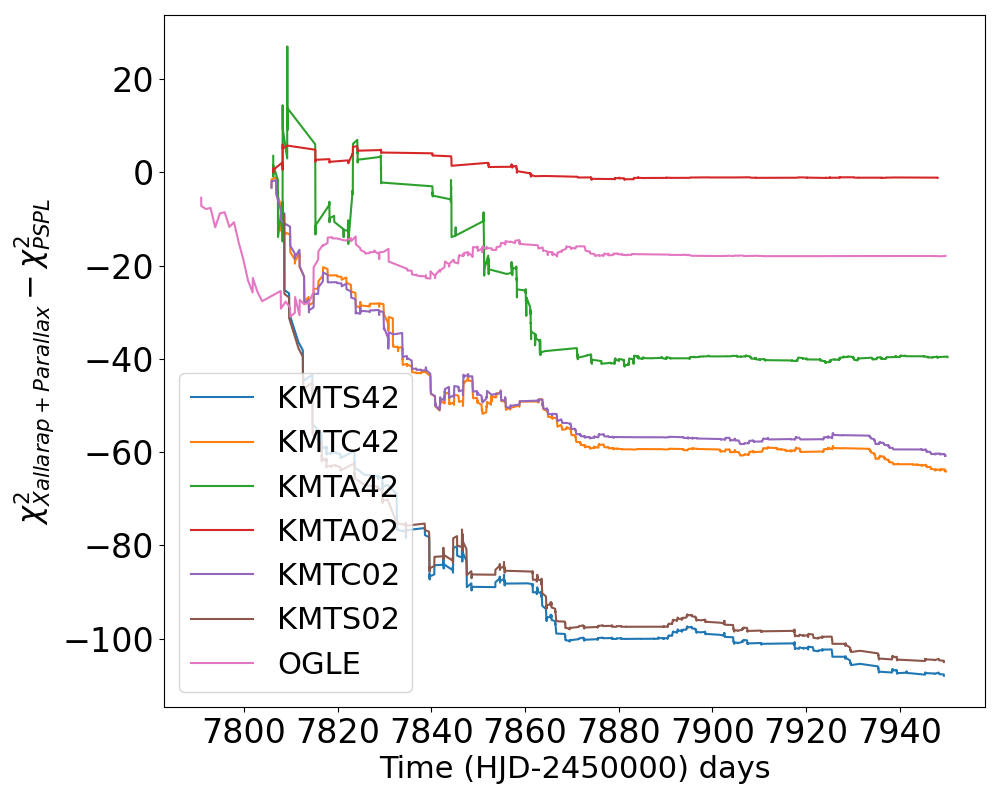
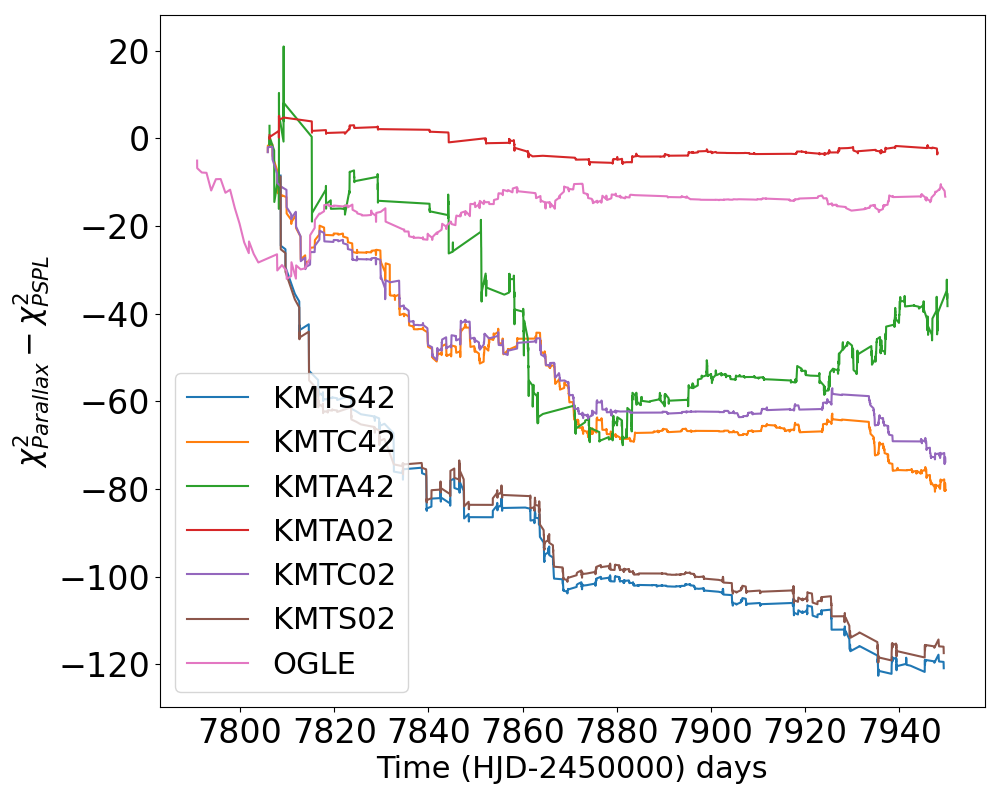
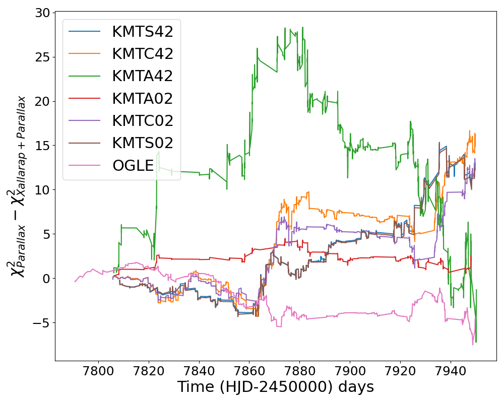
We initially model the light curves with a single lens and binary source xallarap model. For OGLE-2017-BLG-0103, the improves by 6; for OGLE-2017-BLG-0192, the worsens by 60, but the orbital parameters also do not mimic Earth’s orbit. This indicates that the Xallarap model overfits the systematics in the light curve of OGLE-2017-BLG-0192, and the event is not affected by the xallarap effect. But even OGLE-2017-BLG-0103 has only a marginal improvement of . Therefore, we include orbital parallax in our Xallarap model (now known as the Xallarap+Parallax model) for OGLE-2017-BLG-0103. This further reduces the 39. So, our Xallarap+Parallax model converges to a solution with a better of 45 than the orbital parallax model. In Figure (6), we verify the authenticity of the Xallarap signal by plotting the cumulative for three models: the Xallarap+Parallax model compared to the parallax model, the Xallarap+Parallax model compared to the PSPL model, and the orbital parallax model compared to the PSPL model. The Parallax and Xallarap+Parallax models better fit than the PSPL model. We also see that the combined Xallarap+Parallax model shows a marked improvement over the Parallax model alone, as indicated by the positive values for most data sets, particularly KMT-A42. The OGLE dataset does not show significant deviation. So, while the Parallax model gives a better fit than the PSPL model, adding the Xallarap effect further improves the fit.
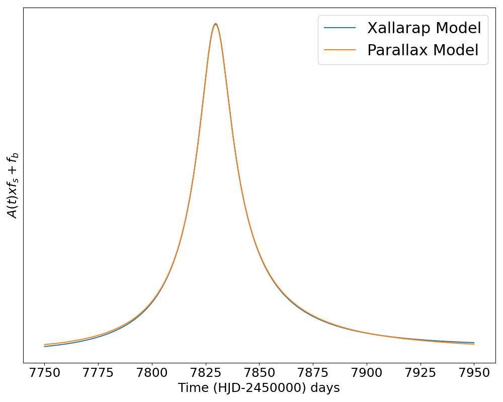
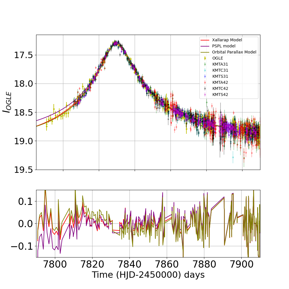
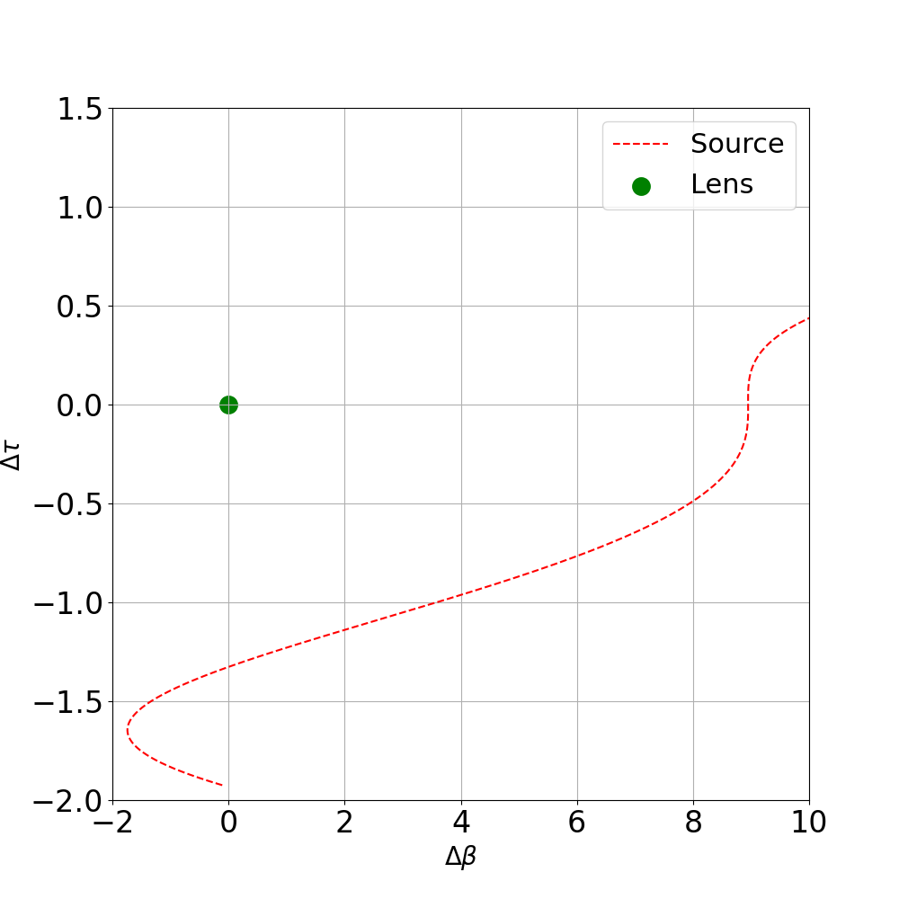
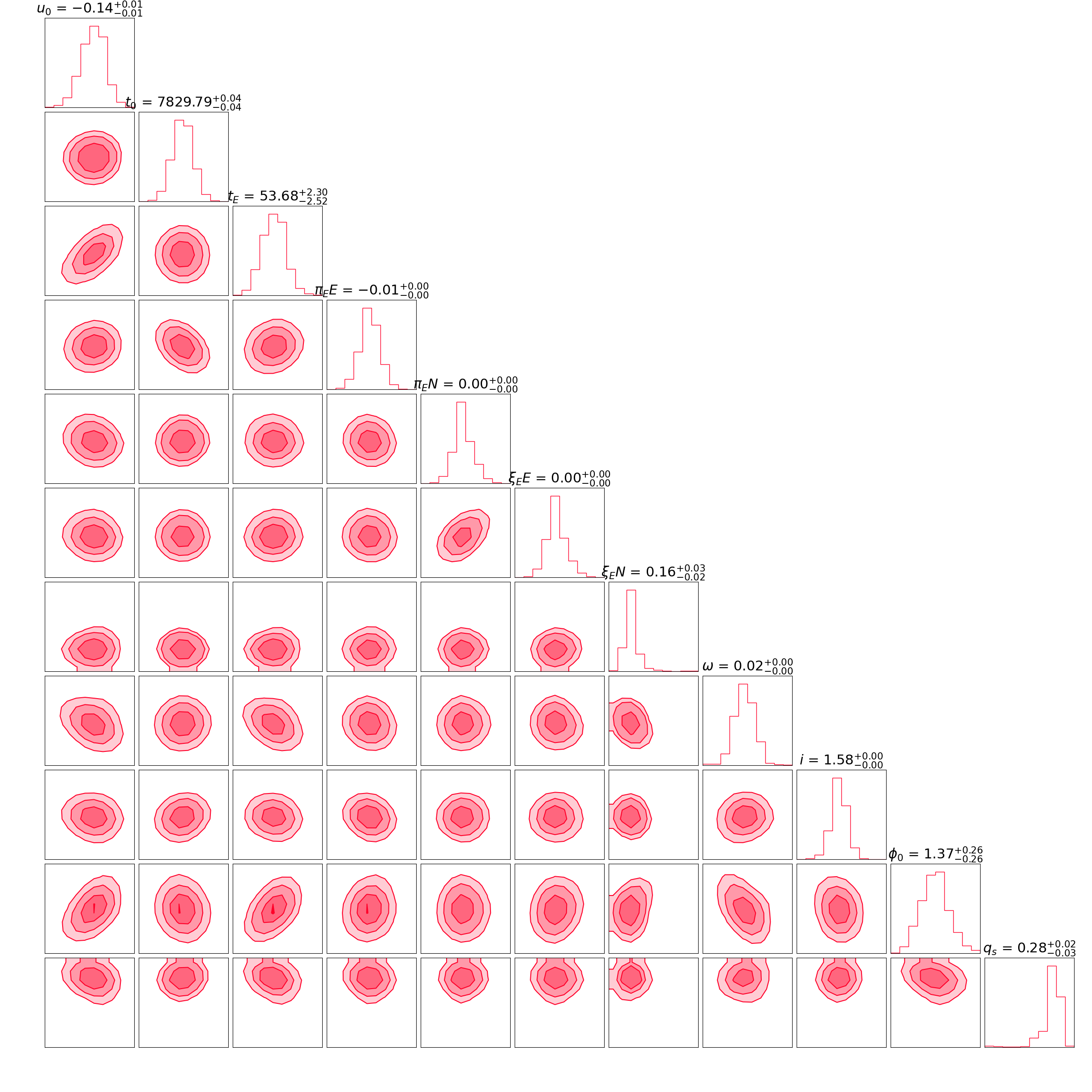
From the model parameters of the event OGLE-2017-BLG-0103 listed in Table (1), we see that the orbital inclination is degrees, the phase angle of the orbit is and the period of the orbit is years. The value of the xallarap vector is , and the orbital parallax also converges to a small value, indicating that the xallarap effect is present in the lightcurve. If we get a xallarap solution miming the Earth’s orbit, the orbital parallax model is favored (Rahvar & Dominik, 2009; Miyazaki et al., 2021). However, our results indicate that we are getting a different orbit that does not reflect Earth’s orbit projected onto the source plane. The mass ratio of the source system () is , which indicates that the companion is not a planetary object. As these values do not mimic the Earth’s orbit, the xallarap solution cannot be ruled out. We show the lightcurve of OGLE-2017-BLG-0103 and the PSPL, Orbital Parallax and Xallarap + Parallax models fitted to it, the residuals plot, the trajectory of the source on the lens plane affected by the best-fit values of and , and the covariance plots in Figure (7).
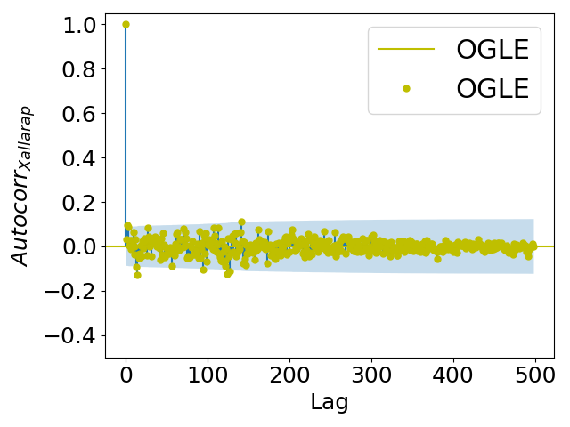
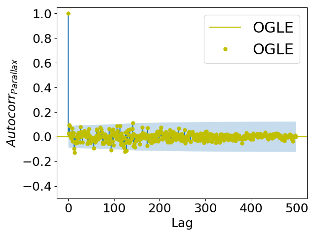
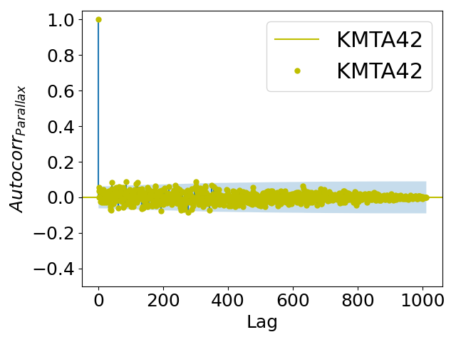
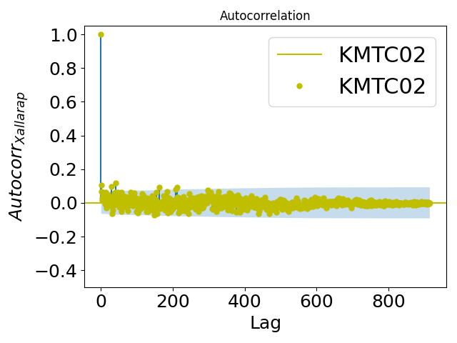
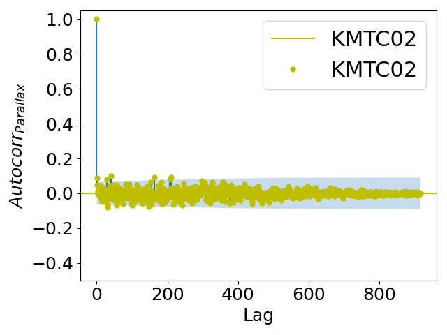
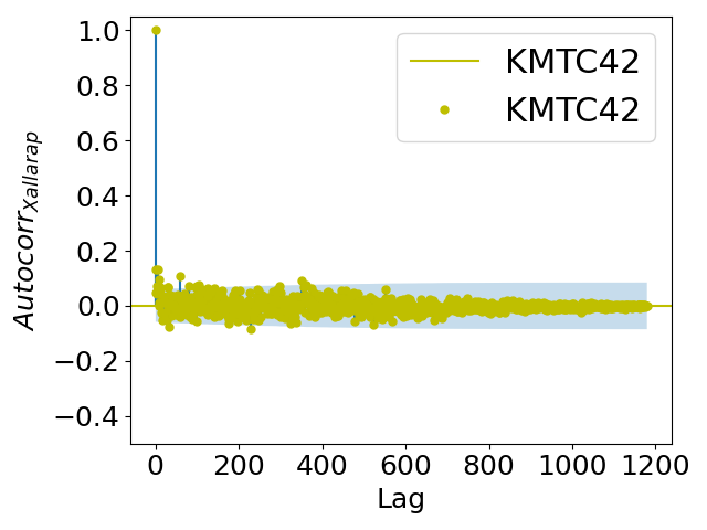
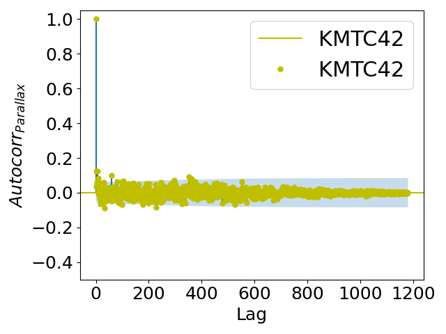
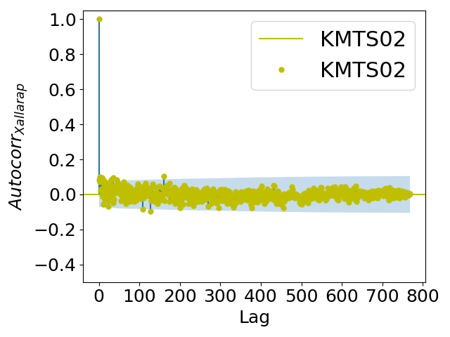
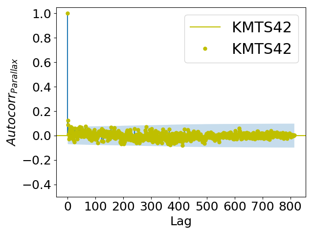
To check whether systematics are playing a role in Xallarap + Parallax model fit, we performed the autocorrelation analysis of the residuals eg. see Figure (8) which shows the autocorrelation vs. time plot for the residuals in OGLE data333The plots for other datasets are shown in Appendix (A)). In all the plots, the ACF at lag 0 is 1, as expected. The autocorrelation values are close to zero for all other lags and lie within the 95% confidence interval (shaded blue region). This indicates that the residuals do not exhibit significant autocorrelation at any lag, suggesting the absence of systematic trends or correlated noise.
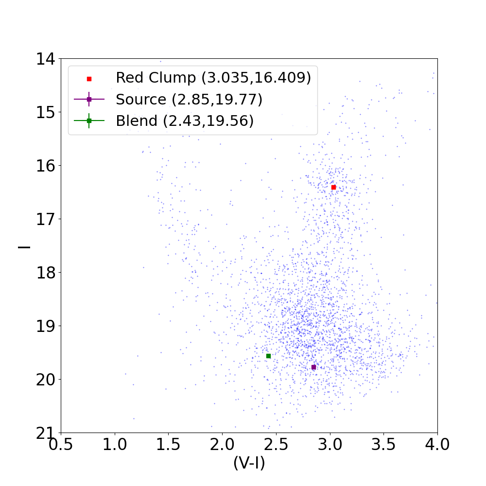
4 Color-Magnitude Diagram for OGLE-2017-BLG-0103
We perform the source analysis only for OGLE-20187-BLG-0103 as we find xallarap signatures in the light curve. In the case of OGLE-2017-BLG-0192, we do not show the CMD here as there are no xallarap signatures in the light curve. Due to adequate coverage of this OGLE-2017-BLG-0103 by different observatories, the source and blend flux are fairly constrained. We then fit the V-band data of the KMTC-BLG42 field to our model and get the values of the source flux and the blend flux in the V-band as we got for the I-band. We use these fluxes to locate the position of the source and the blend on the CMD formed by the stars in the BLG02 field of the KMTC02 dataset (see Figure (9)) and find that the source lies on the main-sequence. The position of the source and the blend on the CMD is () = (2.850.04, 19.770.42), (2.430.03, 19.560.46) respectively. In the CMD, the centroid of the red clump stars in the field, the source, and the blend are shown in red, purple, and green colors, respectively. We can see that the source lies on the main sequence, and the blend is located on the bluer side of the CMD but is slightly brighter than the source. We also find the source in the Gaia DR3 database (Gaia Collaboration et al., 2023) with a source id of 4056392106235284992, source parallax (), equatorial proper motion (, ) = (-2.10 0.73 mas, -8.34 1.11 mas/yr, and -7.15 0.60 mas/yr) respectively. The re-normalized unit weight error () of the source is 1.14, which indicates that the source is a single star or there is no bright companion. The negative value of parallax indicates that the source is faint and heavily blended, which is also evident from the lightcurve and the CMD.
From Nataf et al. (2013), we find that the intrinsic color of the red clump in the bulge is at = (1.06, 14.39). On comparing these values with the values for the centroid of the red clump from pyDIA, we estimate the reddening () and extinction towards the BLG02 field as (2.13,2.10) respectively. This gives the true color and brightness of the source as = (0.710.04, 17.660.42).
5 Lens properties
As mentioned earlier, the modeling of the microlensing light curve does not directly give information about the nature of the lens, e.g., its mass and distance, and it can be measured only if and are measured together from the lightcurve (see Equation (5)). In the case of our events, we do not detect any finite source effects nor have any high-resolution imaging by the Hubble Space Telescope or interferometry observations by VLTI to measure directly. So, we form a galactic model and simulate the microlensing events that could give rise to measured microlensing model parameters eg. and in the case of the Orbital Parallax model and in case of Xallarap+Orbital Parallax model. We formulate the galactic model priors based on the Gaussian velocity distribution towards the bulge (Han & Gould, 1995), stellar density distribution, and the Chabrier stellar mass function (see Chabrier (2003); Batista et al. (2011); Clanton & Gaudi (2014); Zhu et al. (2017); Jung et al. (2018) and others). We assume thin, thick discs with a normalizing factor of 0.12 (Jurić et al., 2008; Jung et al., 2018). We assume the lens and source distances are free parameters in the galactic model. In addition, we assume certain different conditions to obtain the lens mass and distance using Orbital Parallax and Xallarap+Parallax models. Since we have obtained the best fit using the orbital parallax model for both events and another possibility using the Xallarap+Parallax model for OGLE-2017-BLG-0103, we discuss our results of the galactic model for both methods separately.
5.1 Physical properties of the lens for both the events using only the Orbital Parallax model
Here, we discuss the results using the orbital parallax model. Our galactic model is constrained by the samples of and . Since the source star of OGLE-2017-BLG-0103 has proper motion information in Gaia Dr3, we also constrain our galactic model using this information. For this, we transform the proper motion in the galactic plane by referring to the relations by Poleski (2013). However, we cannot constrain the galactic model for OGLE-2017-BLG-0192 as the source star has no astrometry information in Gaia Dr3. So, we use only the and information in this event. The results for OGLE-2017-BLG-0103 are given in Table (3) and the results corresponding to the least model of OGLE-2017-BLG-0192 in Table (4). These tables also show the lens’s proper motion values and expected brightness (assuming it is a main sequence star). The expected brightness includes the extinction towards the lens () computed by using,
| (10) |
where is the extinction to the source (= found in the CMD analysis), and is the scale height of the dust towards the line of sight (see Bennett et al. (2015)). From the result table, we see that for OGLE-2017-BLG-0103, the P1 and P3 pair of solutions give similar results of a very low mass star having a typical of the disc stars while the P2 and P4 pair of solutions give similar results where the lens is more massive and has higher than the disc stars. The expected brightness of these massive lenses computed assuming they lie on the main sequence is brighter than the blend, which is impossible. This indicates the lens might be a stellar-remnant and not a main-sequence star.
5.2 Physical properties of lens and source for OGLE-2017-BLG-0103 using the Xallarap+Parallax model
Our Xallarap+Parallax model consists of a single lens but a binary source. We estimate the source’s mass () using MESA Isochrones and Stellar Evolutionary Tracks (MIST) models (see (Dotter, 2016; Choi et al., 2016) for more information)444Also visit http://waps.cfa.harvard.edu/MIST/index.html to access the database and various tools. its color and brightness information (calculated in the Section (4)) as 1.28. Thus, using Kepler’s third law, we get
| (11) |
where = + , is the orbital period and is the semi-major axis of the orbit. As we know and from our Xallarap+Parallax model, we get =0.980.12 A.U., = and = . Now, is related to by
| (12) |
Thus, we get = 0.16 0.04 mas. Using the galactic model, we can constrain the mass of the lens and distance to it. In our galactic model analysis using the Xallarap+Parallax model, we keep and as free parameters such that is always less than . We use as the upper limit on the lens brightness, assuming that the lens is also a main-sequence star. Since converges to a very small value in the Xallarap+Parallax model, we ignore the parallax constraint555We also do not use Equation (5) as it will lead to a massive lens.. Instead, we use Equation (12). We use the other priors similar to the ones used in the previous galactic model analysis using the Orbital Parallax model. We show the distribution of and in Figure (10). Interestingly, as the xallarap is more sensitive to the lenses closer to the source (Dominik, 1998), the lens moves further and is closer to the source this time than in the earlier galactic model analysis.
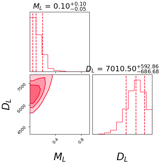
The physical parameters are listed in the last row of Table (3).
| Solution | (kpc) | () | (kpc) | (mas/yr) | () | () | (A.U.) | (years) | |
| P1 | - | - | - | - | |||||
| P2 | - | - | - | - | |||||
| P3 | - | - | - | - | |||||
| P4 | - | - | - | - | |||||
| Xallarap + Parallax | 8.20 |
| Solution | (pc) | () | (pc) | (mas/yr) | |
| P1 |
6 Discussion
In this study, we have analyzed two microlensing events, OGLE-2017-BLG-0103 and OGLE-2017-BLG-0192, to try to identify the nature of the microlens and source. These events peaked close to the vernal equinox in 2017 when the jerk-velocity () and the projected acceleration of the Sun () were very high. This introduces a Jerk-Parallax degeneracy in events with less than 60 days. While this degeneracy is manifested as continuous contours in the plane, for events with slightly longer and higher value of , the degeneracy is converted to a discrete degeneracy (e.g., OGLE-2017-BLG-0103). For even larger , we find that the high value of and splits the contours, and the degeneracy is resolved (e.g., OGLE-2017-BLG-0192).
For OGLE-2017-BLG-0103, while we find that orbital parallax is responsible for the asymmetry in the lightcurve, we also find that the xallarap effect added to the Orbital Parallax model also explains the asymmetry with an improved of 45. The source orbital parameters do not reflect the Earth’s orbit, indicating that the model does not reflect Earth’s orbit on the source plane. When plotted, the cumulative distribution of - plots shows an increasing trend indicating that the xallarap signal is present throughout the lightcurve and is improving the fit. As another quality check, we plotted the autocorrelation of the residuals of the Xallarap+Parallax model at various lags of all the data sets. We found that the correlation of the data is much less, thereby indicating no influence of the systematic trend in the data on the fitted model. This indicates severe tension in both the Orbital Parallax and Xarallarap+Parallax models.
Previous works by Dominik (1998); Smith et al. (2003); Smith (2003); Rahvar & Dominik (2009); Miyazaki et al. (2021) have shown that the xallarap signal is prominent for super-Jupiter mass planets in close orbits. This signal increases with the mass, and the wiggles in the light curve are most visible when the orbital period is small, and the planet’s mass is higher (see Rahvar & Dominik (2009); Miyazaki et al. (2021)).
In the case of OGLE-2017-BLG-0103, the companion is stellar, and the orbital period is ( 0.8 years); hence, we see an asymmetry in the light curve instead of wiggles. Such events are expected to be common during the Nancy Grace Roman Space Telescope era (Spergel et al., 2015), (which was previously named WFIRST) (see Bennett et al. (2018); Penny et al. (2019); Gaudi et al. (2019).
To derive the source properties, we obtained each dataset’s source and the blend fluxes by performing the linear regression of the microlensing model to the data. We use the V-band data of KMTC02 to plot the CMD and then locate the position of the source and the blend on the CMD. The blend is bluer and slightly brighter than the source. Based on its position on the color-magnitude diagram (CMD), we find that the source is a main sequence star.
Given the inherent limitations of the microlensing light curve of both events, which hinder the direct measurement of finite source effects and, consequently, the Einstein radius (), we turned to a galactic model analysis to estimate the mass and distance of the lens. For OGLE-2017-BLG-0192, the galactic model analysis constrained by the samples of and of the best-fitted P1 solution gives 0.1 and located in the near disc. Assuming that the lens is a main-sequence star, we find that it is very faint ( = 24 mag). For OGLE-2017-BLG-0103, we did two separate analyses for the Orbital Parallax and Xallarap+Parallax models. The galactic model for OGLE-2017-BLG-0192 was constrained only by the samples of and . However, the galactic model for OGLE-2017-BLG-0103 was constrained not only by the samples of and , but also the source proper motion () information from Gaia Dr3. The orbital parallax model gives us two similar solutions: one gives a very low-mass main-sequence star in the disc, and the other gives a more massive star and nearer than the former666as predicted by (Gould, 2004), both pairs of Jerk-Parallax solutions give different properties for the lens.. Assuming again that the lens is a main-sequence star, the expected I-band brightness of the lens for the former pair of solutions is 25 mag while it is 18 mag in case of later. If the later pair of solutions are correct, then this will imply that the lens is itself the blend and the lens-source pair can be observed using high-resolution telescopes by the year 2027 (considering the proper motion values given in Table (3)).
The galactic model analysis using the Xallarap+Parallax model shows that the lens is 0.1 dwarf star in the galactic bulge. As expected, our galactic model, constrained by the xallarap signal in the light curve, moves the lens further than the galactic model constrained by only orbital parallax. In our galactic model analysis, we have assumed the source to be located in the bulge at the distance of 8.2kpc. Using MESA isochrone models, we find that the source host has a mass 1.01 and it is orbited by an 0.27 dwarf-star at a separation of 0.98 A.U. and has an orbital period of 0.8 years.
Finally, the question arises: which model is true? Degeneracies are difficult to break in case of single-lens events due to the symmetry in the magnification pattern around the point caustic of the lens. If we apply Ocazm’s razor to the event OGLE-2017-BLG-0103, the orbital parallax model is most likely as it is explained by fewer bodies and a smaller number of parameters. However, the degenerate pairs of orbital parallax solutions also have different lens properties. Rahvar & Dominik (2009) state that an 11.09 is necessary to claim a xallarap detection. In our case, we have a of 45. Moreover, combined orbital parallax and xallarap signals show an increasing trend in the cumulative distribution of the than only the orbital parallax signal. We also do not find any influence from systematics. Indeed, for many microlensing events
of interest, models with xallarap may compete with models with parallax and cannot be excluded easily (e.g., see Miyake et al. (2012), Koshimoto et al. (2017), Rota et al. (2021), Satoh et al. (2023)). The Xallarap+Parallax model could be ruled out if the source has a mass incompatible with the observed flux in follow-up imaging (Bhattacharya et al., 2017, 2020; Blackman et al., 2021). Furthermore, during light curve fitting, if a Xallarap+Parallax model returns an orbital period of 1 year, there is a high chance that the fit has converged to a mirror solution of a parallax model (Dong et al., 2009; Hwang et al., 2011) and then the Xallarap+Parallax model can be discarded. But this is not the case with our model. Also, assuming that the lens is also a main-sequence star, we are finding the brightness of the lens consistent with the blend and source position on the CMD. So, it is difficult to rule out the Xallarap+Parallax model easily. It also is to be noted that all the studies that were previously published using the
Xallarap analysis to date are binary-lens events and this is the first study using a single-lens model.
In this study, we assume that the lens is single because the light curve resembles a Paćzynski curve. If a binary lens would have to produce a similar signal, then assuming the orbital period of 0.8 years and the mass of the lens as 0.1, this would imply a separation (s) of 0.4 A.U. between the lens components. At such a separation, the line caustic formed by a lower mass companion would not go undetected in the light curve. Computing the magnification of a binary lens requires four additional parameters: , , the mass ratio of the lens , and . It also requires solving fifth-order complex polynomials for every pair of and in the parameter space. In addition, parameters and also enter the parameter list when the orbital motion of the lens effect is added to the modeling. Assuming a trajectory angle ()such that the source goes away from the caustic structure would imply a single lens event. Then, involving a secondary lens becomes unnecessary. So, in this work, we have not modeled the lightcurves using a binary lens with an orbital motion effect.
We can expect many such events using the Nancy-Roman Space Telescope mission. While most of the focus of the microlensing community today is to analyze binary or tertiary events, single-lens events with asymmetric light curves need attention to find hidden signatures like OGLE-2017-BLG-0103. It is difficult to address any Xallarap solution as the source is faint, cannot be resolved using the current survey telescopes, and is usually in the bulge. So, a program for future AO observations using powerful large aperture telescopes like the Thirty Meter Telescope (Sanders, 2013; Skidmore et al., 2015) can be made to study the degenerate solutions. Such observations can potentially validate the lens’s mass and distance obtained using the galactic model constrained by various microlensing parameters.
Acknowledgement
Sarang Shah is thankful to the India-TMT Coordination Center at the Indian Institute of Astrophysics for providing the time and resources to complete the analysis of this microlensing event. This work started as a part of the PhD thesis submitted to the University of Canterbury. This research has made use of data (https://kmtnet.kasi.re.kr/ulens/) from the KMTNet system (Kim et al. 2016) operated by the Korea Astronomy and Space Science Institute (KASI) at three host sites of CTIO in Chile, SAAO in South Africa, and SSO in Australia. Data transfer from the host site to KASI was supported by the Korea Research Environment Open NETwork (KREONET).
Appendix A Autocorrelation results of Xallarap and Parallax models
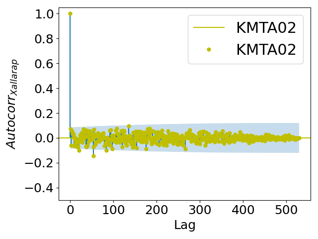
In this section, we show the auto-correlation of the residuals calculated for the whole duration of the lightcurve for the KMTNet dataset. The residuals are the difference between the Xallarap+Parallax model and the observed data. The auto-correlation is 1 at lag 0, which is expected. However, as the lag value increases, the auto-correlation values for all the datasets drop and are consistently close to 0 and within the confidence interval throughout.


References
- Alard & Lupton (1998) Alard, C., & Lupton, R. H. 1998, apj, 503, 325, doi: 10.1086/305984
- Albrow (2017) Albrow. 2017, doi: 10.5281/zenodo.268049
- Alcock et al. (1995a) Alcock, C., Allsman, R. A., Alves, D., et al. 1995a, apjl, 454, L125, doi: 10.1086/309783
- Alcock et al. (1995b) Alcock, C., Allsman, R. A., Axelrod, T. S., et al. 1995b, ApJ, 445, 133, doi: 10.1086/175678
- An et al. (2002) An, J. H., Albrow, M. D., Beaulieu, J.-P., et al. 2002, apj, 572, 521, doi: 10.1086/340191
- Aubourg et al. (1994) Aubourg, E., Bareyre, P., Bréhin, S., et al. 1994, in The Dark Side of the Universe - Experimental Efforts and Theoretical Framework, 69
- Bagheri et al. (2019) Bagheri, F., Sajadian, S., & Rahvar, S. 2019, MNRAS, 490, 1581, doi: 10.1093/mnras/stz2682
- Batista et al. (2011) Batista, V., Gould, A., Dieters, S., et al. 2011, aap, 529, A102, doi: 10.1051/0004-6361/201016111
- Bennett et al. (2002a) Bennett, D. P., Becker, A. C., Calitz, J. J., et al. 2002a, ArXiv Astrophysics e-prints
- Bennett et al. (1993) Bennett, D. P., Akerlof, C., Alcock, C., et al. 1993, in Texas/PASCOS ’92: Relativistic Astrophysics and Particle Cosmology, ed. C. W. Akerlof & M. A. Srednicki, Vol. 688, 612, doi: 10.1111/j.1749-6632.1993.tb43945.x
- Bennett et al. (2002b) Bennett, D. P., Becker, A. C., Quinn, J. L., et al. 2002b, apj, 579, 639, doi: 10.1086/342225
- Bennett et al. (2015) Bennett, D. P., Bhattacharya, A., Anderson, J., et al. 2015, apj, 808, 169, doi: 10.1088/0004-637X/808/2/169
- Bennett et al. (2018) Bennett, D. P., Akeson, R., Anderson, J., et al. 2018, arXiv e-prints, arXiv:1803.08564, doi: 10.48550/arXiv.1803.08564
- Bhattacharya et al. (2017) Bhattacharya, A., Bennett, D. P., Anderson, J., et al. 2017, apj, 154, 59, doi: 10.3847/1538-3881/aa7b80
- Bhattacharya et al. (2020) Bhattacharya, A., Bennett, D. P., Beaulieu, J. P., et al. 2020, arXiv e-prints, arXiv:2009.02329, doi: 10.48550/arXiv.2009.02329
- Blackman et al. (2021) Blackman, J. W., Beaulieu, J. P., Cole, A. A., et al. 2021, AJ, 161, 279, doi: 10.3847/1538-3881/abfda3
- Bond et al. (2001) Bond, I. A., Abe, F., Dodd, R. J., et al. 2001, mnras, 327, 868, doi: 10.1046/j.1365-8711.2001.04776.x
- Bond et al. (2002) —. 2002, mnras, 331, L19, doi: 10.1046/j.1365-8711.2002.05374.x
- Bozza et al. (2021) Bozza, V., Khalouei, E., & Bachelet, E. 2021, MNRAS, 505, 126, doi: 10.1093/mnras/stab1376
- Bramich et al. (2013) Bramich, D. M., Horne, K., Albrow, M. D., et al. 2013, mnras, 428, 2275, doi: 10.1093/mnras/sts184
- Carroll & Ostlie (2017) Carroll, B. W., & Ostlie, D. A. 2017, An introduction to modern astrophysics, Second Edition
- Chabrier (2003) Chabrier, G. 2003, pasp, 115, 763, doi: 10.1086/376392
- Choi et al. (2016) Choi, J., Dotter, A., Conroy, C., et al. 2016, apj, 823, 102, doi: 10.3847/0004-637X/823/2/102
- Clanton & Gaudi (2014) Clanton, C., & Gaudi, B. S. 2014, apj, 791, 91, doi: 10.1088/0004-637X/791/2/91
- Delplancke et al. (2001) Delplancke, F., Górski, K. M., & Richichi, A. 2001, A&A, 375, 701, doi: 10.1051/0004-6361:20010783
- Dominik (1998) Dominik, M. 1998, A&A, 329, 361, doi: 10.48550/arXiv.astro-ph/9702039
- Dong et al. (2009) Dong, S., Gould, A., Udalski, A., et al. 2009, apj, 695, 970, doi: 10.1088/0004-637X/695/2/970
- Dong et al. (2019) Dong, S., Mérand, A., Delplancke-Ströbele, F., et al. 2019, ApJ, 871, 70, doi: 10.3847/1538-4357/aaeffb
- Dotter (2016) Dotter, A. 2016, apjs, 222, 8, doi: 10.3847/0067-0049/222/1/8
- Einstein (1936) Einstein, A. 1936, Science, 84, 506, doi: 10.1126/science.84.2188.506
- Foreman-Mackey et al. (2013) Foreman-Mackey, D., Hogg, D. W., Lang, D., & Goodman, J. 2013, Publications of the Astronomical Society of the Pacific, 125, 306, doi: 10.1086/670067
- Gaia Collaboration et al. (2023) Gaia Collaboration, Vallenari, A., Brown, A. G. A., et al. 2023, A&A, 674, A1, doi: 10.1051/0004-6361/202243940
- Gaudi et al. (2019) Gaudi, B. S., Akeson, R., Anderson, J., et al. 2019, BAAS, 51, 211, doi: 10.48550/arXiv.1903.08986
- Gould (1992) Gould, A. 1992, apj, 392, 442, doi: 10.1086/171443
- Gould (1994) —. 1994, ApJ, 421, L71, doi: 10.1086/187190
- Gould (2004) —. 2004, apj, 606, 319, doi: 10.1086/382782
- Gould et al. (1994) Gould, A., Miralda-Escude, J., & Bahcall, J. N. 1994, apjl, 423, L105, doi: 10.1086/187247
- Gould et al. (2009) Gould, A., Udalski, A., Monard, B., et al. 2009, apjl, 698, L147, doi: 10.1088/0004-637X/698/2/L147
- Griest & Hu (1992) Griest, K., & Hu, W. 1992, apj, 397, 362, doi: 10.1086/171793
- Han & Gould (1995) Han, C., & Gould, A. 1995, apj, 447, 53, doi: 10.1086/175856
- Han & Gould (1997) —. 1997, ApJ, 480, 196, doi: 10.1086/303944
- Hog et al. (1995) Hog, E., Novikov, I. D., & Polnarev, A. G. 1995, A&A, 294, 287
- Hwang et al. (2011) Hwang, K.-H., Han, C., Udalski, A., et al. 2011, mnras, 413, 1244, doi: 10.1111/j.1365-2966.2011.18206.x
- Jiang et al. (2004) Jiang, G., DePoy, D. L., Gal-Yam, A., et al. 2004, apj, 617, 1307, doi: 10.1086/425678
- Jung et al. (2018) Jung, Y. K., Hwang, K.-H., Ryu, Y.-H., et al. 2018, apj, 156, 208, doi: 10.3847/1538-3881/aae319
- Jurić et al. (2008) Jurić, M., Ivezić, Ž., Brooks, A., et al. 2008, apj, 673, 864, doi: 10.1086/523619
- Kim et al. (2018) Kim, H.-W., Hwang, K.-H., Shvartzvald, Y., et al. 2018, arXiv e-prints, arXiv:1806.07545. https://arxiv.org/abs/1806.07545
- Kim et al. (2016) Kim, S.-L., Lee, C.-U., Park, B.-G., et al. 2016, KMTNet: A Network of 1.6m Wide-Field Optical Telescopes Installed at Three Southern Observatories,Journal of Korean Astronomical Society, 49, 37, doi: 10.5303/JKAS.2016.49.1.037
- Koshimoto et al. (2017) Koshimoto, N., Udalski, A., Beaulieu, J. P., et al. 2017, apj, 153, 1, doi: 10.3847/1538-3881/153/1/1
- Mao et al. (2002) Mao, S., Smith, M. C., Woźniak, P., et al. 2002, mnras, 329, 349, doi: 10.1046/j.1365-8711.2002.04986.x
- Miyake et al. (2012) Miyake, N., Udalski, A., Sumi, T., et al. 2012, apj, 752, 82, doi: 10.1088/0004-637X/752/2/82
- Miyazaki et al. (2021) Miyazaki, S., Johnson, S. A., Sumi, T., et al. 2021, AJ, 161, 84, doi: 10.3847/1538-3881/abcec2
- Nataf et al. (2013) Nataf, D. M., Gould, A., Fouqué, P., et al. 2013, apj, 769, 88, doi: 10.1088/0004-637X/769/2/88
- Nemiroff & Wickramasinghe (1994) Nemiroff, R. J., & Wickramasinghe, W. A. D. T. 1994, ApJ, 424, L21, doi: 10.1086/187265
- Paczynski (1986) Paczynski, B. 1986, apj, 304, 1, doi: 10.1086/164140
- Paczynski (1997) —. 1997, arXiv e-prints, astro, doi: 10.48550/arXiv.astro-ph/9711007
- Park et al. (2004) Park, B.-G., DePoy, D. L., Gaudi, B. S., et al. 2004, apj, 609, 166, doi: 10.1086/420926
- Penny et al. (2019) Penny, M. T., Gaudi, B. S., Kerins, E., et al. 2019, The Astrophysical Journal Supplement Series, 241, 3, doi: 10.3847/1538-4365/aafb69
- Poindexter et al. (2005) Poindexter, S., Afonso, C., Bennett, D. P., et al. 2005, apj, 633, 914, doi: 10.1086/468182
- Poleski (2013) Poleski, R. 2013, arXiv e-prints, arXiv:1306.2945, doi: 10.48550/arXiv.1306.2945
- Rahvar & Dominik (2009) Rahvar, S., & Dominik, M. 2009, MNRAS, 392, 1193, doi: 10.1111/j.1365-2966.2008.14120.x
- Rota et al. (2021) Rota, P., Hirao, Y., Bozza, V., et al. 2021, AJ, 162, 59, doi: 10.3847/1538-3881/ac0155
- Sahu et al. (2022) Sahu, K. C., Anderson, J., Casertano, S., et al. 2022, ApJ, 933, 83, doi: 10.3847/1538-4357/ac739e
- Sanders (2013) Sanders, G. H. 2013, Journal of Astrophysics and Astronomy, 34, 81, doi: 10.1007/s12036-013-9169-5
- Satoh et al. (2023) Satoh, Y. K., Koshimoto, N., Bennett, D. P., et al. 2023, AJ, 166, 116, doi: 10.3847/1538-3881/ace908
- Skidmore et al. (2015) Skidmore, W., TMT International Science Development Teams, & Science Advisory Committee, T. 2015, Research in Astronomy and Astrophysics, 15, 1945, doi: 10.1088/1674-4527/15/12/001
- Skowron et al. (2011) Skowron, J., Udalski, A., Gould, A., et al. 2011, apj, 738, 87, doi: 10.1088/0004-637X/738/1/87
- Smith (2003) Smith, M. C. 2003, mnras, 343, 1172, doi: 10.1046/j.1365-8711.2003.06753.x
- Smith et al. (2003) Smith, M. C., Mao, S., & Paczyński, B. 2003, mnras, 339, 925, doi: 10.1046/j.1365-8711.2003.06183.x
- Soszyński et al. (2001) Soszyński, I., Żebruń, K., Woźniak, P. R., et al. 2001, apj, 552, 731, doi: 10.1086/320582
- Spergel et al. (2015) Spergel, D., Gehrels, N., Baltay, C., et al. 2015, arXiv e-prints, arXiv:1503.03757. https://arxiv.org/abs/1503.03757
- Sumi et al. (2003) Sumi, T., Abe, F., Bond, I. A., et al. 2003, apj, 591, 204, doi: 10.1086/375212
- Udalski et al. (1994) Udalski, A., Szymanski, M., Kaluzny, J., et al. 1994, actaa, 44, 227
- Udalski et al. (2015) Udalski, A., Szymański, M. K., & Szymański, G. 2015, actaa, 65, 1. https://arxiv.org/abs/1504.05966
- Witt & Mao (1995) Witt, H. J., & Mao, S. 1995, apjl, 447, L105, doi: 10.1086/309566
- Yoo et al. (2004) Yoo, J., DePoy, D. L., Gal-Yam, A., et al. 2004, apj, 603, 139, doi: 10.1086/381241
- Zhu et al. (2017) Zhu, W., Udalski, A., Calchi Novati, S., et al. 2017, apj, 154, 210, doi: 10.3847/1538-3881/aa8ef1