Harnessing the Intrinsic Knowledge of Pretrained Language Models
for Challenging Text Classification Settings

Abstract

Text classification, a classic task in natural language processing (NLP), involves assigning predefined categories to textual data and is crucial for applications ranging from sentiment analysis to spam detection. This thesis advances text classification by harnessing the intrinsic knowledge of Pretrained Language Models (PLMs) to address three challenging scenarios: distractor selection for multiple-choice cloze questions, improving robustness for prompt-based zero-shot text classification, and demonstration selection for retrieval-based in-context learning.

Firstly, we focus on selecting distractors for multiple-choice cloze questions, ensuring that they are misleading yet incorrect. We assess the relationship between human experts’ annotations (accept/reject) and various features, including context-free features (e.g., word frequency) and context-sensitive features (e.g., conditional probabilities of fill-in-the-blank words). We utilize pretrained embeddings and follow annotation instructions for context-free feature design, and we find that using contextualized word representations from PLMs as features drastically improves performance over traditional feature-based models, even rivaling human performance (Chapter 3).

Secondly, prompt-based zero-shot approaches are highly sensitive to the choice of prompts, even with task descriptions. We propose to exploit the intrinsic knowledge of the model by providing domain-independent label descriptions. We craft small datasets that describe task labels with related terms, short templates, dictionary definitions, and more. This approach achieves an average improvement of 17-19% in accuracy over traditional zero-shot methods across multiple datasets. It is robust to variations in patterns and verbalizers and proves effective across different text domains, even outperforming few-shot out-of-domain learning in multiple settings (Chapter 4).

Lastly, we consider PLMs’ existing knowledge of the task-specific label space of both in-context learning demonstrations and test inputs. We find that using demonstrations that are misclassified by the models, particularly those that lie near the decision boundary of the test examples, leads to better performance. Additionally, considering output label space is more important than semantic similarity, and our methods help reduce model confusion. Extensive experiments on fine-grained classification tasks show that our method improves F1 macro scores by up to 2.6% over traditional retriever-based approaches (Chapter 5).

In conclusion, by leveraging contextualized word representations for distractor selection, and focusing on zero-shot and few-shot tasks that emphasize strategic demonstration selection, this thesis demonstrates the effective use of PLMs to enhance performance and robustness in text classification.

Computer Science Computer Science 7

Chapter 1 Introduction

Consider a news article that begins with “Climate scientists tell a conference that greater efforts should be made to pull $CO_{2}$ from the atmosphere.” Where would it be categorized? Most likely, under Tech News rather than Sports News. Similarly, the title of an email might indicate whether it is a scam, and the correctness of a math problem solution can be judged given the question and answer.

These scenarios highlight the essence of text classification—a fundamental task in natural language processing (NLP) where the objective is to assign predefined categories to a piece of text, whether it be a phrase, a sentence, a paragraph, or a series of long documents [2]. Text classification is ubiquitous in daily life, underpinning a broad range of applications from sentiment analysis to toxic text filtering. At the same time, it could be challenging due to the complex dependencies and inherent ambiguity of natural language.

Traditional text classification models often require extensive labeled datasets and manual feature engineering. To classify a series of textual inputs, we first map them to real-valued vectors, a process known as feature extraction [2]. Early models heavily relied on manually designed features, and often benefited from traditional pretrained word representations such as Word2Vec [3, 4] and GloVe [5]. These static word embeddings map the discrete words to continuous vector space, and maintain intrinsic pretrained knowledge, such as word analogies (e.g., “king” - “man” + “woman” $\approx$ “queen”). However, these static word embeddings fail to capture the context-dependent nature of polysemous words, and the small-scale models trained from scratch often struggle with generalization and require large, domain-specific labeled datasets to achieve satisfactory performance, especially on complex tasks.

Recent advancements in deep learning, particularly in transformer architecture [6] and large-scale pretraining, have achieved inspiring success in NLP fields. Pretrained language models (PLMs), such as ELMo [8], GPT-2 [9] and BERT [10], have demonstrated the ability to capture intricate patterns within large corpora and retain vast amounts of knowledge during training [11, 12]. They can be used directly or adapted as needed to enhance text classification tasks, and their encoded intrinsic knowledge facilitates strong performance in zero-shot scenarios, where we don’t have available training data.

In this thesis, we explore three challenging settings in text classification, focusing particularly on harnessing PLMs and leveraging their intrinsic knowledge for the task. These settings are:

• Distractor Analysis and Selection for Multiple-Choice Cloze Questions (Section 1.1). To tackle the challenge of generating misleading yet incorrect distractors for cloze questions, we develop models that utilize features designed with internal word representations derived from PLMs.

• Label-Description Training for Zero-Shot Text Classification (Section 1.2). To address the difficulty of generalizing to unseen labels, we craft small finetuning datasets that describe task labels. This approach significantly improves model robustness and performance by exploiting the models’ intrinsic knowledge.

• Ambiguity-Aware In-Context Learning with Large Language Models (Section 1.3). To deal with the sensitivity of PLMs to prompts in in-context learning, we select effective demonstrations by considering misclassified demonstrations and resolving model ambiguity about test example labels.

Detailed discussions of these settings and our contributions are provided in the subsequent sections.

1.1 Feature engineering with PLMs for distractor selection

Distractor selection involves determining whether an incorrect answer (distractor) is plausible enough to challenge the test-taker without making the question unanswerable. Consider this cloze question: "The bank will           its customers of the new policy." with its correct answer being "notify". We need to decide whether "collaborate" is a good distractor here. Compared to predicting correct answers, designing questions with appropriate distractors is more complex. While we can retrieve questions and correct answers from plain text, selecting optimal distractors—those that are similar to the correct answers but still incorrect [13]—is challenging.

In real-world scenarios, the annotators who select the distractors are often domain experts following specific instructions that could be transformed into features. In practice, a feature-based lightweight model is sometimes preferred. But how do we design a feature-based lightweight model while using the PLMs’ knowledge at the same time? How much gain would the PLMs bring?

Feature engineering is the practice of constructing or selecting suitable features with domain knowledge to improve model performance [14]. For this cloze question task, the features could be one or more words before or after the blank, part-of-speech (POS) tags of the previous word, frequency of the candidate words, etc. While we could directly input word frequency to the model, the text needs to be mapped to appropriate representations.

In contrast to static word embeddings, contextualized word representations derived from PLMs are functions of the entire textual input [11], making them context-sensitive and potentially better for feature design. For instance, the polysemous word “bank” could refer to either a river bank or a financial bank by itself, which could be disambiguated from the context in the example mentioned above.

To achieve a deeper understanding of context, PLMs typically share the common objective of predicting or reconstructing tokens based on contextual information during pretraining tasks. Encoder-only models, such as BERT and its variants, utilize a “Masked Language Model (MLM)” pretraining objective. It involves randomly masking some input tokens and predicting them based on the surrounding context, similar to an open cloze-style question. For the cloze question example in this section, we could make predictions with BERT by computing the conditional probabilities of the candidate “collaborate” in the given contexts. The conditional probabilities can be seen as features and combined across multiple models for the final prediction.

Past work often lacks direct supervision for training, making it challenging to develop and evaluate automatic methods for distractor selection. In this thesis, we experiment on two datasets of multiple-choice cloze questions (MCQs) for second-language learners, where the distractor selections are manually annotated by human experts. As it is a binary classification task, it could be turned into a ranking problem and auto-suggests candidates for human experts.

We assess the relationship between annotators’ choices and features based on distractors and the correct answers, both with and without the surrounding passage context in the cloze questions. We find that simple features of the distractor and correct answer correlate with the annotations, though using PLMs to measure the fit of the distractor in the context additionally offers substantial benefits. Based on these analyses, we also propose and train models to automatically select distractors and quantitatively measure the importance of model components. Our contributions are:

• We design a range of features, both context-free and context-sensitive, and find that they weakly correlate with human annotations.

• We develop and train models by combining simple features with advanced contextualized word representations from PLMs. Our strongest models are able to approach or even exceed human performance.

• We provide a detailed quantitative analysis of the importance of various model components, offering insights into how different features contribute to performance.

1.2 Improving robustness for prompt-based zero-shot classification

The emergence of PLMs has given rise to a pretrain-and-finetune paradigm [15], which achieves impressive performance but typically requires labeled data from downstream tasks. In zero-shot text classification, where such datasets are unavailable, it becomes challenging for models to generalize to new, unseen labels during training.

One approach to address this challenge is to provide the model with task descriptions, exploiting the intrinsic knowledge of PLMs to solve zero-shot tasks without supervision [16, 12, 17, 18, 19]. The core idea is transforming text classification into language modeling, i.e., prompt-based classification.

Among the various prompt-based methods, the pattern-verbalizer approach [18] (detailed in Section 2.2.2) is a notable example. It converts the task into a cloze question to match the pretraining task format. In this method, a pattern constructs the prompt from the textual input with a single mask token, and the verbalizer maps each label to a word from the model’s vocabulary. For instance, to classify the restaurant review “Overpriced, salty and overrated!”, a pattern like “the restaurant is [MASK]” is appended to the review. The model then predicts the most probable verbalizer (e.g., “good” for positive sentiment and “bad” for negative) for the [MASK] position. While this approach is commonly associated with encoder-based models like RoBERTa [20], autoregressive models can generate the next word or phrase based on the prompt, adhering to the same underlying idea of prompt-based classification.

While effective, this approach is highly sensitive to the choice of patterns and verbalizers, and minor changes in the wording of the prompt can lead to significant variations in model performance [21, 22, 23, 24]. This sensitivity has led to the development of prompt engineering to find the most appropriate prompt for better performance, however, the best practices vary by task [25]. Additionally, despite advancements in understanding task descriptions, models still face challenges with the representation of labels in text classification. To avoid irrelevant answers, researchers often make predictions by comparing the conditional probabilities of pre-defined strings. However, this approach may suffer from various biases, including surface form competition [26], where probability is distributed among various valid strings, including those that differ trivially, such as by capitalization.

To mitigate the sensitivity of the models, we curate small finetuning datasets intended to describe the labels for a task. Unlike typical finetuning data, which has texts annotated with labels, our data describes the labels in language, e.g., using a few related terms, dictionary or encyclopedia entries, and short templates. Our method works for both MLM-style models and autoregressive models, as the data can be used for finetuning as well as in-context learning, where it is included in the textual prompts. This approach is domain-independent, easily adaptable to most use cases, and improves model robustness and performance. Our contributions are:

• Across a range of topic and sentiment datasets, our method is more accurate than zero-shot by 17-19% absolute.

• It is more robust to choices required for zero-shot classification, such as patterns for prompting the model to classify and mappings from labels to tokens in the model’s vocabulary.

• Since our data merely describes the labels but does not use input texts, finetuning on it yields a model that performs strongly on multiple text domains for a given label set, even improving over few-shot out-of-domain classification in multiple settings.

1.3 Demonstration selection for in-context learning

In-context learning (ICL) is a tuning-free approach where the input-output examples (known as demonstrations) are concatenated with the textual input [17]. ICL preserves the generality of the LLMs as it doesn’t change the model parameters [27]. However, the length of the input prompt is usually limited, and only a few demonstrations could be included. Since PLMs are sensitive to the prompts, selecting good demonstrations becomes a crucial research question.

One effective strategy is leveraging semantic similarity between the ICL demonstrations and test examples with a text retriever [28]. The retriever can either be an off-the-shelf one such as [29, 30, 31, 32], or a retriever trained specifically for that task [33, 28]. Compared to a static set of demonstrations, this dynamic and context-sensitive approach leads to substantial improvements and makes PLMs less sensitive to factors such as demonstration ordering [34].

However, Lyu et al. [35] indicates that there is a copy effect where the language model’s predictions are significantly influenced by demonstration inputs that closely resemble the test input. This suggests that the retrieval-based approach depends heavily on the retriever. Off-the-shelf retrievers may not be ideal for some tasks, and tuning the retriever involves a finetuning process similar to traditional finetuning, which undermines the tuning-free benefit of ICL. Additionally, this approach can be sub-optimal without considering the PLM’s existing knowledge about the task, especially with respect to the output label space.

Motivated by uncertainty sampling—a technique in active learning where the model selects the data points it is most uncertain about—we aim to resolve model ambiguity about test example labels in this thesis by conducting zero-shot experiments in advance.

Through extensive experimentation on three text classification tasks, we find that including demonstrations that the LLM previously mis-classified and also fall near the test example’s decision boundary, brings the most performance gain. Our contributions are:

• We develop an ICL method that considers model ambiguity regarding both demonstration and test example labels.

• We add constraints incrementally in our experiments on fine-grained topic and sentiment classification tasks, showing that our method outperforms the retrieval-based ICL on two different model sizes.

• We observe that semantically similar demonstrations tend to share the same gold label as the test example, and filtering them with the set of the top two most likely labels offers a more accurate approximation. This insight sheds light on retrieval-based ICL’s effectiveness and contributes to the success of our proposed method.

1.4 Organization of the Thesis

The thesis is organized as follows:

• Chapter 2: Background of pretrained language models’ architectures and text classification approaches with PLMs that are adopted in this thesis, including the pattern-verbalizer approach and in-context learning.

• Chapter 3: Distractor Analysis and Selection for Multiple-Choice Cloze Questions for Second-Language Learners. It presents the challenges of selecting effective distractors and details the method and the performance gain of utilizing contextualized word representations from PLMs for features. This chapter is based on [36].

• Chapter 4: Label-Description Training for Zero-Shot Text Classification. It explains the creation of small finetuning datasets that describe task labels for topic and sentiment classification. This chapter is based on [37].

• Chapter 5: Ambiguity-Aware In-Context Learning with Large Language Models. It shows that using PLM’s existing knowledge, such as the model prediction of demonstrations and test examples, is important to improve model performance and resolve model ambiguity. This chapter is based on [38].

• Chapter 6: Summary of the thesis, including a synthesis of the contributions and potential future work.

Chapter 2 Text Classification with Pretrained Language Models

This chapter provides an overview of the architectures of pretrained language models (PLMs) and existing approaches for text classification tasks using PLMs.

2.1 Pretrained Language Models

Pretrained language models are language models that have been trained on large-scale corpora using self-supervised learning techniques [15]. While there is a rich history of work in using large-scale language models [39, 40] and pretraining [41, 42], the widespread adoption and use of PLMs as the default tool for NLP began with the introduction of ELMo [8]. Subsequently, it was further popularized by a series of work such as GPT [43] and BERT [44]. The primary training target of these models involves predicting or reconstructing tokens based on contextual information. This approach aligns with two crucial aspects of language use from a psycholinguistics perspective: comprehension (the ability to understand) and production (the ability to generate).

2.1.1 ELMo

ELMo (Embeddings from Language Models) was introduced in 2018 as a novel type of deep contextualized word representation rather than a model for finetuning. However, it improved the state of the art on several NLP benchmarks by integrating deep contextual word representations with existing task-specific architectures.

ELMo is constructed using a bidirectional language model (biLM) and a task-specific layer. The biLM is constructed by two LSTM (Long Short-Term Memory) networks [45]: one is in the forward direction and one in the backward direction. Assume we are given a series of textual inputs $\{x_{1},\cdots,x_{N}\}$, these LSTM networks predict the probability of a token $x_{t}$ given its history and future context, respectively, as shown below:

$$p(x_{1},x_{2},\cdots,x_{N})=\sum_{t=1}^{N}p(x_{t}|x_{1},x_{2},\cdots,x_{t-1})$$

$$p(x_{1},x_{2},\cdots,x_{N})=\sum_{t=1}^{N}p(x_{t}|x_{t+1},x_{t+2},\cdots,x_{N})$$

In the pretraining process, the token representations and softmax layer parameters of the two LSTMs are tied, and the objective is to maximize the joint log-likelihood of both the forward and backward directions. When used for a downstream task, the contextualized word representation can be obtained through a learned linear combination of all the layer representations of the word. As ELMo adopts two LSTM layers, the first layer is more suitable for part-of-speech (POS) tagging, while the second layer is better for word sense prediction.

This makes ELMo a feature-based approach, as the ELMo representations are typically used as additional input features for other models. However, the authors of ELMo also mention that finetuning the biLM on domain-specific data improves model performance in some cases.

2.1.2 GPT and BERT

Feature engineering played a crucial role in early NLP tasks, leading researchers to initially use pretrained language models’ (PLMs) contextualized embeddings for feature design. However, as PLMs have become increasingly powerful, the necessity for extensive feature engineering has diminished.

GPT.

GPT (Generative Pre-trained Transformer) is a unidirectional (left-to-right) decoder-based model, making it particularly well-suited for natural language generation tasks. GPT uses token and absolute positional embeddings to map input text into a vector space, and the embeddings are directly input to the decoder without the encoder structure. It is trained autoregressively to predict the next token given a sequence of textual inputs, but its transformer layers can also serve as contextualized representations.

Unlike ELMo, which applies task-specific layers on top of the pretrained representations, GPT aims to learn a universal representation and requires minimal changes to the model architecture when transferring to new tasks. For the classification task given a series of textual inputs $\{x_{1},\cdots,x_{N}\}$, and the corresponding labels $\{y_{1},\cdots,y_{c}\}\in\mathcal{L}$, where $\mathcal{L}$ is the set of all possible labels, the following loss, which includes a weight $\lambda$, is applied:

$$L=\sum_{(x,y)}\log P(y|x_{1},\cdots,x_{N})+\lambda\sum_{t}\log P(x_{t}|x_{1},\cdots,x_{t-1})$$

After proposing GPT, OpenAI scaled up the model parameter size, used more data for pretraining, and introduced GPT-2 [9] and GPT-3 [47] with a few modifications. They emphasized the importance of unsupervised multitask learning in Radford et al. [9] and introduced “in-context learning” in Brown et al. [47].

BERT.

BERT (Bidirectional Encoder Representations from Transformers), on the other hand, is an encoder-based model. It is bi-directional, with all layers conditioned on both left and right context. Compared to GPT, BERT has an advantage in tasks that require incorporating context from both directions.

BERT is pretrained on two unsupervised tasks: Masked LM and binarized next sentence prediction (NSP). For the Masked LM (MLM) task (a cloze-style training objective that is crucial for training this bidirectional language model), 15% of the tokens are randomly sampled for prediction. To mitigate possible mismatch between pretraining and finetuning data, the sampled token in the input can be:

• Replaced by a special token [MASK] (80%)

• Replaced by a random token (10%)

• Left unchanged (10%)

As BERT doesn’t include the transformer decoder, it uses an MLM head to predict the masked token. Regarding special tokens aside from [MASK], BERT inserts a [CLS] token at the beginning of every input example, which can be used for sentence-level classification with a classification head. It also uses a [SEP] token as a separator to distinguish between text segments, such as sentences.

BERT can be used in a feature-based manner without finetuning, as each transformer layer in BERT provides a contextualized representation of each token. A common approach is to combine these layers with a weighted sum.

Comparison to ELMo.

Unlike ELMo, which follows a feature-based approach, GPT and BERT belong to the finetuning approach. Another key difference lies in their model architectures: GPT and BERT are built on the transformer architecture [6], whereas ELMo adopts LSTM.

The original transformer architecture consists of an encoder and a decoder, where the encoder extracts features from the textual input, and the decoder uses these features to produce the output. GPT and BERT utilize different parts of the transformer architecture: GPT is decoder-based, while BERT is encoder-based.

2.1.3 Other Recent PLMs

With the field’s rapid evolution, many PLMs have been introduced for both general usage and specific domains, such as finance [48] and medicine [49]. Due to their scaled-up parameter sizes, these models are often referred to as large language models (LLMs) rather than PLMs.

Regarding model architectures, a few modern variants of BERT, such as RoBERTa and DeBERTa [50], are commonly used as encoder-based models for tasks such as text classification and natural language inference. Encoder-decoder models, such as T5 [51] and BART [52], are suitable for sequence-to-sequence (seq2seq) tasks, such as machine translation and text summarization. Many recent LLMs are decoder-based, e.g., GPT-3.5 [53], the Llama series [54, 55, 56], and Google’s PaLM and PaLM 2 [19, 57]. Reasons for the popularity of decoder-only models at large scale may include their simpler architecture, strong zero-shot generalization after self-supervised training [58], and ease of use for general-purpose generation tasks [59].

2.2 Text Classification with PLMs

Text classification involves assigning predefined categories to textual data. Finetuning on in-domain data generally achieves good performance [60]. However, the increasing size of PLMs makes finetuning challenging. Additionally, the lack of sufficient data in specific domains for finetuning has prompted research into data-efficient methods [61, 62], addressing zero-shot or few-shot scenarios. Zero-shot refers to situations where the model is tested on new classes or tasks it hasn’t seen during training, and few-shot refers to scenarios where only a few examples are available for the task (or class) of interest.

2.2.1 Finetuning

The finetuning approach involves adjusting the model’s parameters or implementing techniques like prompt tuning or parameter-efficient methods (e.g., adapters [63], LoRA [64], and QLoRA [65]) to minimize parameter changes. This approach is also used to calibrate pretrained models to reduce biases [66]. However, finetuning potentially makes the model to become less generalizable. For example, a question-answering model may not achieve high performance on a classification task [67].

One method to address this is instruction-tuning [67, 68, 69], where the model is finetuned on multiple tasks and datasets to learn to follow instructions, thereby enhancing cross-task generalization. This method is different from multi-task finetuning, as ablation studies show that natural instructions are crucial [68]. Prepending inputs with natural language instructions yields better zero-shot results compared to using the task and dataset names; moreover, using inputs without any templates leads to the worst performance [68].

Improving the model’s ability to follow instructions will also help it adapt to the user’s needs to perform specific tasks, especially for those unlikely to appear naturally in the unsupervised pre-training data. In Wei et al. [68], they phrase the natural language inference (NLI) task as a more natural question, which achieves better performance. Another common approach to aligning models with human preferences is reinforcement learning with human feedback (RLHF) [70], which is often conducted after instruction tuning. Recently, some work has adopted high-quality synthetic feedback data generated by LLMs [71].

While these finetuning methods have achieved great success, Zhou et al. [72] argue that only a limited amount of high-quality instruction tuning data is necessary to align models with human preferences and end tasks, as LLMs acquire vast knowledge during the pretraining process.

2.2.2 Prompting

Prompting involves providing a language model with a textual input (prompt) in inference time to perform tasks. The content of a prompt depends on the use case and can include task descriptions/instructions and input-output examples. This approach leverages the pretrained capabilities of the model to handle various tasks without gradient updates. However, the model is sensitive to the input prompts [24, 23, 73], which can be challenging for practitioners to design effectively in true zero-shot settings.

Pattern-verbalizer Approach.

The pattern-verbalizer approach [18] is a prompt-based method suitable for zero-shot and few-shot scenarios. However, its main advantage lies in data efficiency.

This approach transforms text classification into a language modeling task, utilizing the pretrained capabilities of models like BERT. For example, given a restaurant review, a prompt might be “[CLS] Overpriced, salty and overrated! The restaurant is [MASK]. [SEP]” The model predicts the masked word based on the context, mapping it to a predefined label using a verbalizer. These verbalizers, such as “great” for positive reviews or “awful” for negative reviews, should be semantically related to the corresponding labels.

It is known that this approach is sensitive to the pattern and verbalizer choices. When Schick and Schütze [18] focuses more on combining different prompt patterns, Gao et al. [74] explores automatically generating prompts and selecting the verbalizer. They also consider including demonstrations (input-output pairs) in the prompt when finetuning over a small number of examples. For instance, consider the following: “[CLS] Overpriced, salty and overrated! It was [MASK]. [SEP] A beautiful park. It was great. [SEP] No reason to watch. It was awful. [SEP]”

In-Context Learning Approach.

In-context learning (ICL) is a tuning-free approach where the demonstrations are concatenated with the textual input [17]. It is similar to the pattern-verbalizer approach, but it focuses on leveraging the model’s ability to generalize from a few examples without updating model parameters. LLMs can better follow instructions, and finetuning them is often expensive or impossible due to limited access to model parameters. This makes ICL an effective and flexible approach.

Recent studies show that ICL demonstrations (input-output pairs) are primarily used for specifying the domain and format [75, 76, 35], and ICL demonstrations selection and ordering both influenced the effectiveness [77, 29, 73]. However, retrieval-based ICL, which selects a set of demonstrations for each test example using a retriever, has shown advantages in both robustness and performance [27].

The retriever’s objectives often focus on either similarity (mainly semantic similarity) [33, 31] or diversity [78, 79]. Selecting demonstrations based on semantic similarity (or term matching) ensures that the examples are relevant and contextually appropriate, and there are also works based on structural similarity, such as [80]. On the other hand, emphasizing diversity in demonstration selection helps in exposing the model to varied examples, potentially enhancing its robustness and adaptability.

2.3 Summary

In this chapter, we give an overview of PLMs’ architectures used in this thesis, and existing approaches (both finetuning and prompting) for text classification tasks with PLMs. In Chapter 3, we address the challenges of selecting distractors for cloze questions using contextualized word representations derived from PLMs. In Chapter 4, we tackle the issue of model sensitivity to prompts and propose the use of small finetuning datasets. In Chapter 5, we focus on improving the selection of demonstrations in prompting, proposing a solution to model ambiguity by considering model predictions.

Chapter 3 Distractor Analysis and Selection for Multiple-Choice Cloze Questions for Second-Language Learners

In this chapter, we focus on selecting distractors for multiple-choice cloze questions, i.e., deciding whether a candidate is selected or not with a binary classifier. This task is challenging because the distractors should be attractive enough to mislead test-takers, yet still be incorrect in terms of the knowledge being tested. In our case, it is a mixture of vocabulary knowledge and contextual understanding, and the distractors could be either semantically or syntactically inappropriate, contributing to the difficulty. Moreover, annotated data has inherent limitations because there is no single right choice; instead, many choices are possible. This variability makes traditional supervised learning challenging. However, pretrained language models could naturally pick up on signals from their training corpora that correlate with distractor quality. We can then leverage this pretrained knowledge with a small amount of supervised data.

Given the complexity of the selection rules, we design a range of features, both context-free and context-sensitive, including contextualized word representations from PLMs. Remarkably, our strongest model matches human performance.

This chapter is based on [36].

3.1 Introduction

Multiple-choice cloze questions (MCQs) are widely used in examinations and exercises for language learners [81]. The quality of MCQs depends not only on the question and choice of blank, but also on the choice of distractors, i.e., incorrect answers. While great improvements are achieved in question answering and reading comprehension, selecting good distractors is still a problem. Different from selecting the best ones in most of the NLP tasks, distractors, which could be phrases or single words, are incorrect answers that distract students from the correct ones.

According to Pho et al. [82], distractors tend to be syntactically and semantically homogeneous with respect to the correct answers. Distractor selection may be done manually through expert curation or automatically using simple methods based on similarity and dissimilarity to the correct answer [83, 84]. Intuitively, optimal distractors should be sufficiently similar to the correct answers in order to challenge students, but not so similar as to make the question unanswerable [85]. However, past work usually lacks direct supervision for training, making it difficult to develop and evaluate automatic methods. To overcome this challenge, Liang et al. [81] sample distractors as negative samples for the candidate pool in the training process, and Chen et al. [86] sample questions and use manual annotation for evaluation.

In this thesis, we experiment on two datasets of MCQs for second-language learners with distractor selections annotated manually by human experts. Both datasets consist of instances with a sentence, a blank, the correct answer that fills the blank, and a set of candidate distractors. Each candidate distractor has a label indicating whether a human annotator selected it as a distractor for the instance. The first dataset, which we call MCDSent, contains solely the sentence without any additional context, and the sentences are written such that they are understandable as standalone sentences. The second dataset, MCDPara, contains sentences drawn from an existing passage and therefore also supplies the passage context.

dataset	context with correct answer	distractor	label
MCDSent	How many people are planning to attend the party?	contribute	T
	The large automobile manufacturer has a factory near here.	beer	F
	The large automobile manufacturer has a factory near here.	corporation	F
	The large automobile manufacturer has a factory near here.	apartment	T
MCDPara	Stem cells are special cells that can divide to produce many different kinds of cells. When they divide, the new cells may be the same type of cell as the original cell….	plastic	F
	…These circumstances made it virtually impossible for salmon to mate. Therefore, the number of salmon declined dramatically.	thousands	T

Table 3.1: Example instances from MCDSent and MCDPara. Contexts are shown and correct answers are bold and underlined. Part of the paragraph contexts are replaced by ellipses.

To analyze the datasets, we design context-free features of the distractor and the correct answer, including length difference, embedding similarities, frequencies, and frequency rank differences. We also explore context-sensitive features, such as probabilities from large-scale pretrained models like BERT [44]. In looking at the annotations, we found that distractors are unchosen when they are either too easy or too hard (i.e., too good of a fit in the context). Consider the examples in Table 3.1. For the sentence “The large automobile manufacturer has a factory near here.”, “beer” is too easy and “corporation” is too good of a fit, so both are rejected by annotators. We find that the BERT probabilities capture this tendency; that is, there is a nonlinear relationship between the distractor probability under BERT and the likelihood of annotator selection.

We develop and train models for automatic distractor selection that combine simple features with representations from pretrained models like BERT and ELMo [8]. Our results show that the pretrained models improve performance drastically over the feature-based models, leading to performance rivaling that of humans asked to perform the same task. By analyzing the models, we find that the pretrained models tend to give higher score to grammatically-correct distractors that are similar in terms of morphology and length to the correct answer, while differing sufficiently in semantics so as to avoid unanswerability.

3.2 Related Work

Existing approaches to distractor selection use WordNet [87] metrics [88, 86], word embedding similarities [89], thesauruses [90, 91], and phonetic and morphological similarities [92]. Other approaches consider grammatical correctness, and introduce structural similarities in an ontology [93], and syntactic similarities [94]. When using broader context, bigram or $n$-gram co-occurrence [95, 96], context similarity [83], and context sensitive inference [97] have also been applied to distractor selection.

Based on these heuristic features, Liang et al. [81] assemble these features and apply neural networks, training the model to predict the answers within a lot of candidates. Yeung et al. [85] further applies BERT for ranking distractors by masking the target word. As we have two manually annotated datasets that have different lengths of contexts, we adopt both word pair features and the context-specific distractor probabilities to build our feature-based models. Moreover, we build both ELMo-based and BERT-based models, combining them with our features and measuring the impact of these choices on performance.

3.3 Datasets

We define an instance as a tuple $\langle x,c,d,y\rangle$ where $x$ is the context, a sentence or paragraph containing a blank; $c$ is the correct answer, the word/phrase that correctly fills the blank; $d$ is the distractor candidate, the distractor word/phrase being considered to fill the blank; and $y$ is the label, a true/false value indicating whether a human annotator selected the distractor candidate. We use the term question to refer to a set of instances with the same values for $x$ and $c$.

3.3.1 Data Collection

We build two datasets with different lengths of context. The first, which we call MCDSent (“Multiple Choice Distractors with SENTence context”), uses only a single sentence of context. The second, MCDPara (“Multiple Choice Distractors with PARAgraph context”), has longer contexts (roughly one paragraph).

Our target audience is Japanese business people with TOEIC level 300-800, which translates to pre-intermediate to upper-intermediate level. Therefore, words from two frequency-based word lists, the New General Service List (NGSL; [98]) and the TOEIC Service List (TSL; [99]), were used as a base for selecting words to serve as correct answers in instances. A proprietary procedure was used to create the sentences for both MCDSent and MCDPara tasks, and the paragraphs in MCDPara are excerpted from stories written to highlight the target words chosen as correct answers. The sentences are created following the rules below:

• A sentence must have a particular minimum and maximum number of characters.

• The other words in the sentence should be at an equal or easier NGSL frequency level compared with the correct answer.

• The sentence theme should be business-like.

All the MCDSent and MCDPara materials were created in-house by native speakers of English, most of whom hold a degree in Teaching English to Speakers of Other Languages (TESOL).

3.3.2 Distractor Annotation

We now describe the procedure used to propose distractors for each instance and collect annotations regarding their selection.

A software tool with a user interface was created to allow annotators to accept or reject distractor candidates in MCDSent and MCDPara. Distractor candidates are sorted automatically for presentation to annotators in order to favor those most likely to be selected. The distractor candidates are drawn from a proprietary dictionary, and those with the same part-of-speech (POS) as the correct answers (if POS data is available) are preferred. Moreover, the candidates that have greater similarity to the correct answers are preferred, such as being part of the same word learning section in the language learning course and the same NGSL word frequency bucket. There is also preference for candidates that have not yet been selected as distractors for other questions in the same task type and the same course unit.

After the headwords are decided through this procedure, a morphological analyzer is used to generate multiple inflected forms for each headword, which are provided to the annotators for annotation. Both the headwords and inflected forms are available when computing features and for use by our models.

Six annotators were involved in the annotation, all of whom are native speakers of English. Out of the six, four hold a degree in TESOL. Selecting distractors involved two-step human selection. An annotator would approve or reject distractor candidates suggested by the tool, and a different annotator, usually more senior, would review their selections. The annotation guidelines for MCDSent and MCDPara follow the same criteria. The annotators are asked to select distractors that are grammatically plausible, semantically implausible, and not obviously wrong based on the context. Annotators also must accept a minimum number of distractors depending on the number of times the correct answer appears in the course. Table 3.1 shows examples from MCDSent and MCDPara along with annotations.

3.3.3 Annotator Agreement

Some instances in the datasets have multiple annotations, allowing us to assess annotator agreement. We use the term “sample” to refer to a set of instances with the same $x$, $c$, and $d$. Table 3.2 shows the number of samples with agreement and disagreement for both datasets. Samples with only one annotation dominate the data. Of the samples with multiple annotations, nearly all show agreement.

# annotators	MCDSent			MCDPara
	agree	disagree	total	agree	disagree	total
1	-	-	232256	-	-	734063
2	2553	122	2675	9680	152	9841
3	121	2	123	493	3	496
4	17	0	17	62	0	62
5	10	0	10	12	0	12
6	0	0	0	2	0	2

Table 3.2: Numbers of samples for which annotators agree or disagree.

3.3.4 Distractor Phrases

While most distractors are words, some are phrases, including 16% in MCDSent and 13% in MCDPara. In most cases, the phrases are constructed by a determiner or adverb (“more”, “most”, etc.) and another word, such as “most pleasant”, “more recently”, and ‘More Utility’. However, some candidates show other patterns, such as noun phrases “South Pole”, erroneously-inflected forms “come ed” and other phrases (e.g. “Promises Of”, “No one”).

3.3.5 Dataset Preparation

We randomly divided each dataset into train, development, and test sets. We remind the reader that we define a “question” as a set of instances with the same values for the context $x$ and correct answer $c$, and in splitting the data we ensure that for a given question, all of its instances are placed into the same set. The dataset statistics are shown in Table 3.3. False labels are much more frequent than true labels, especially for MCDPara.

dataset	type	$y$	train	dev	test	total
MCDSent	questions	-	2,713	200	200	3,113
	instances	T	30,737	1,169	1,046	32,952
		F	191,908	6,420	6,813	205,141
		total	222,645	7,589	7,859	238,093
MCDPara	questions	-	14,999	1,000	1,000	16,999
	instances	T	49,575	597	593	50,765
		F	688,804	7,620	8,364	704,788
		total	738,379	8,217	8,957	755,553

Table 3.3: Dataset sizes in numbers of questions (a “question” is a set of instances with the same $x$ and $c$) and instances, broken down by label ($y$) and data split.

3.4 Features and Analysis

We now analyse the data by designing features and studying their relationships with the annotations.

3.4.1 Features

We now describe our features. The dataset contains both the headwords and inflected forms of both the correct answer $c$ and each distractor candidate $d$. In defining the features below based on $c$ and $d$ for an instance, we consider separate features for two types of word pairs:

• headword pair: correct answer headwords and candidate headwords

• inflected form pair: correct answer and candidate

For features that require embedding words, we use the 300-dimensional GloVe word embeddings [100] pretrained on the 42 billion token Common Crawl corpus. The GloVe embeddings are provided in decreasing order by frequency, and some features below use the line numbers of words in the GloVe embeddings, which correspond to frequency ranks. For words that are not in the GloVe vocabulary, their frequency ranks are $|N|+1$, where $N$ is the size of the GloVe vocabulary. We use the four features listed below:

• length difference: absolute value of length difference (in characters, including whitespace) between $c$ and $d$.

• embedding similarity: cosine similarity of the embeddings of $c$ and $d$. For phrases, we average the embeddings of the words in the phrase.

• distractor frequency: negative log frequency rank of $d$. For phrases, we take the max rank of the words (i.e., the rarest word is chosen).

• freq. rank difference: feature capturing frequency difference between $c$ and $d$, i.e., $\log(1+\left\lvert r_{c}-r_{d}\right\rvert)$ where $r_{w}$ is the frequency rank of $w$.

feature	MCDSent		MCDPara
	head	infl	head	infl
length difference	-0.116	-0.171	-0.145	-0.173
embedding similarity	-0.018	0.026	-0.014	0.016
candidate frequency	-0.057	0.113	-0.062	0.028
freq. rank difference	-0.048	-0.161	-0.033	-0.091

Table 3.4: Spearman correlations with T/F choices, where “head” denotes headword pairs, and “infl” denotes inflected form pairs.

3.4.2 Correlations of Features and Annotations

The Spearman correlations between feature values and labels are presented in Table 3.4. We compute Spearman correlations between features and the T/F annotations, mapping the T/F labels to 1/0 for computing correlations. The overall correlations are mostly close to zero, so we explore how the relationships vary for different ranges of feature values below. Nonetheless, we can make certain observations about the correlations:

• Length difference has a weak negative correlation with annotations, which implies that the probability of a candidate being selected decreases when the absolute value of word length difference between the candidate and correct answer increases. The same conclusion can be drawn with headword pairs although the correlation is weaker.

• Embedding similarity has a very weak correlation (even perhaps none) with the annotations. However, the correlation for headwords is slightly negative while that for inflected forms is slightly positive, suggesting that annotators tend to select distractors with different lemmas than the correct answer, but similar inflected forms (e.g., for the instance “I   many cakes to find a good one.” where the correct answer is “tasted”, “taste” and “tastes” are both rejected, while “borrowed”, “inspired” and “hired” are selected).

• Candidate frequency also has a very weak correlation with annotations (negative for headwords and positive for inflected forms). Since the feature is the negative log frequency rank, a distractor with a rare headword but more common inflected form is more likely to be selected, at least for MCDSent.

• Frequency rank difference has a weak negative correlation with annotations, and this trend is more significant with the inflected form pair. This implies that annotators tend to select distractors in the same frequency range as the correct answers.

The correlations are not very large in absolute terms, however we found that there were stronger relationships for particular ranges of these feature values and we explore this in the next section.

3.4.3 Label-Specific Feature Histograms

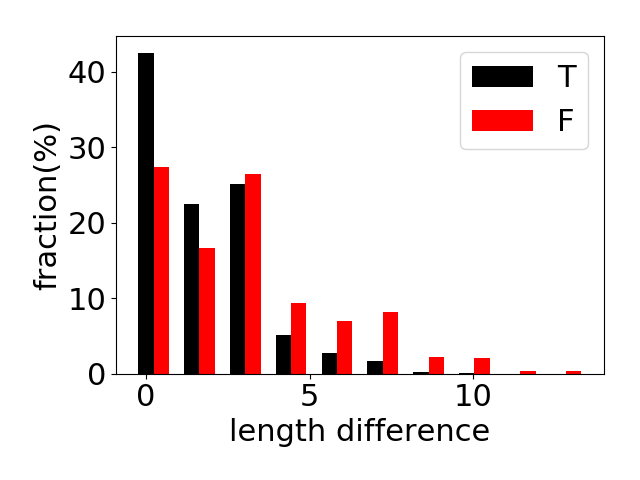
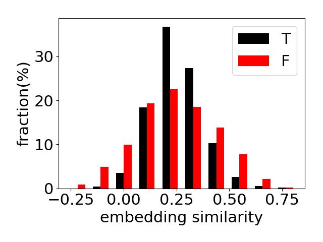
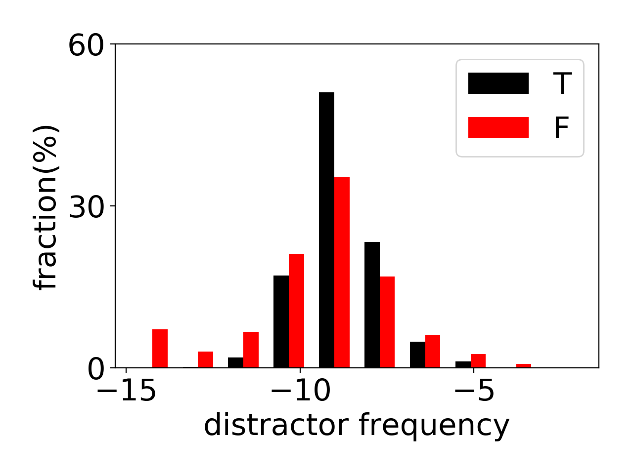
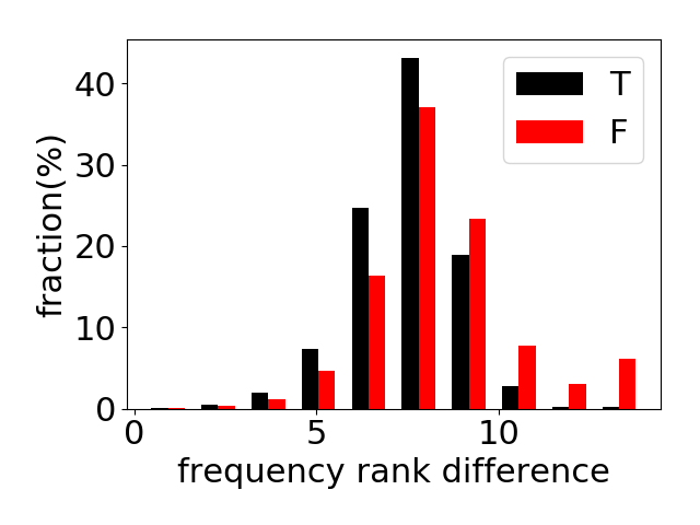
Figure 3.1: Label-specific feature histograms for MCDSent (inflected form pairs).

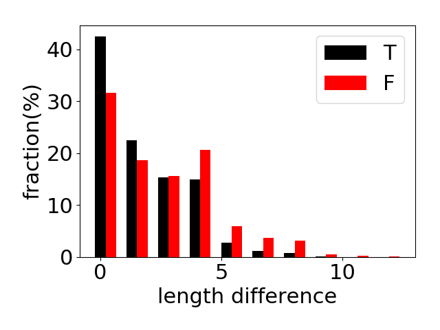
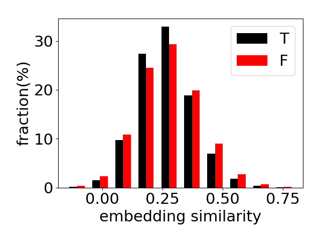
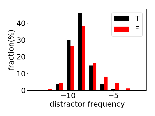
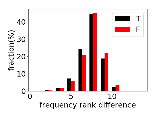
Figure 3.2: Label-specific feature histograms for MCDSent (headword pairs).

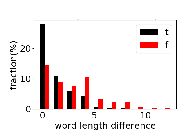
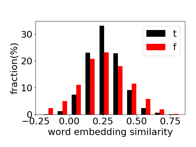
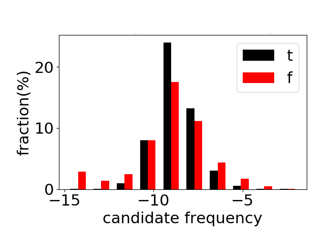
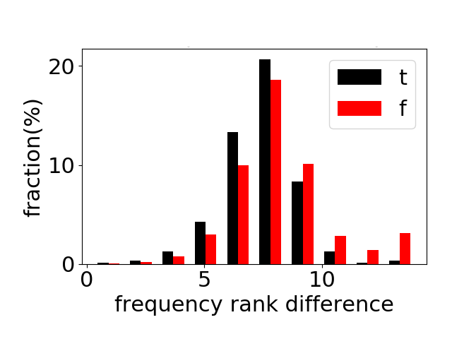
Figure 3.3: Label-specific feature histograms for MCDPara (inflected form pairs).

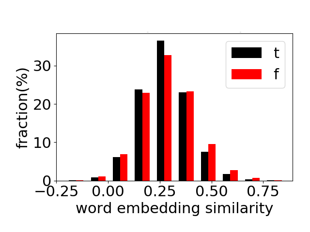
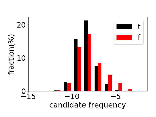
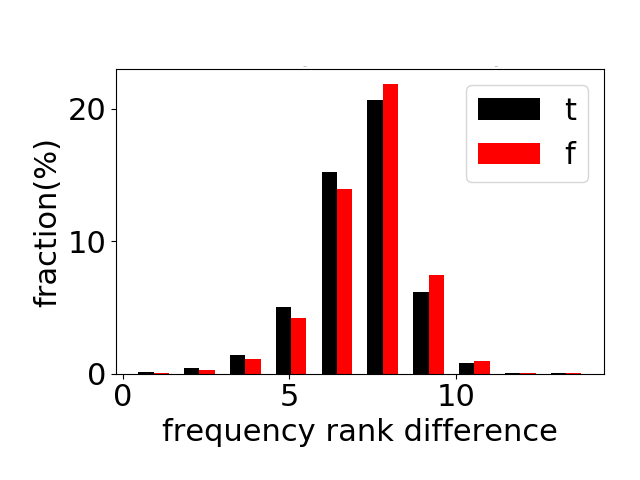
Figure 3.4: Label-specific feature histograms for MCDPara (headword pairs).

Figure 3.1 - 3.4 shows histograms of feature values for each label on inflected form pairs and headword pairs for MCDSent and MCDPara. Since the data is unbalanced, the histograms are “label-normalized”, i.e., normalized so that the sum of heights for each label is 1. So, we can view each bar as the fraction of that label’s instances with feature values in the given range. Given that the figures exhibit common trends, we will discuss them below, using Figure 3.1 and 3.2 as an example. We make several observations:

• The annotators favor candidates that have approximately the same length as the correct answers (Fig. 3.1, plot 1), as the true bars are much higher in the first bin (length difference 0 or 1), which accords with the correlations in the previous section.

• Selected distractors have moderate embedding similarity to the correct answers (Fig. 3.1, plot 2). If cosine similarity is very high or very low, then those distractors are much less likely to be selected. Such distractors are presumably too difficult or too easy, respectively. These trends are much clearer for the inflected forms.

• Selected distractors are moderately frequent (Fig. 3.1, plot 3). Very frequent and very infrequent distractors are less likely to be selected. More common words are to the right of the plot. Compared to candidate headwords, there are more rare words among candidates (the heights of the bars rise to the far left under the inflected form setting), which are mainly annotated as false. These tend to be erroneously-inflected and correctly-inflected-but-extremely-rare forms, which annotators do not select.

• Distractors with small frequency rank differences (those on the left of plot 4) are more likely to be chosen (Fig. 3.1, plot 4). Large frequency differences tend to be found with very rare distractors, some of which may be erroneously-inflected forms.

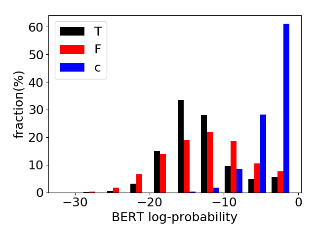
Figure 3.5: Histograms of BERT log-probabilities of selected distractors (“T”), unselected distractors (“F”), and correct answers (“$c$”) in MCDSent.

3.4.4 Probabilities of Distractors in Context

We use BERT [44] to compute probabilities of distractors and correct answers in the given contexts in MCDSent. We insert a mask symbol in the blank position and compute the probability of the distractor or correct answer at that position. Figure 3.5 shows histograms for correct answers and distractors (normalized by label). The correct answers have very high probabilities. The distractor probabilities are more variable and the shapes of the histograms are roughly similar for the true and false labels. Interestingly, however, when the probability is very high or very low, the distractors tend to not be selected. The selected distractors tend to be located at the middle of the probability range. This pattern shows that BERT’s distributions capture (at least partially) the nonlinear relationship between goodness of fit and suitability as distractors.

3.5 Models

Since the number of distractors selected for each instance is uncertain, our datasets could be naturally treated as a binary classification task for each distractor candidate. We now present models for the task of automatically predicting whether a distractor will be selected by an annotator. We approach the task as defining a predictor that produces a scalar score for a given distractor candidate. This score can be used for ranking distractors for a given question, and can also be turned into a binary classification using a threshold. We define three types of models, described in the subsections below.

3.5.1 Feature-Based Models

Using the features described in Section 3.4, we build a simple feed-forward neural network classifier that outputs a scalar score for classification. Only inflected forms of words are used for features without contexts, and all features are concatenated and used as the input of the classifier. For features that use BERT, we compute the log-probability of the distractor and the log of its rank in the distribution. For distractors that consist of multiple subword units, we mask each individually to compute the above features for each subword unit, then use the concatenation of mean, min, and max pooling of the features over the subword units. We refer to this model as $M_{\textit{feat}}$.

3.5.2 ELMo-Based Models

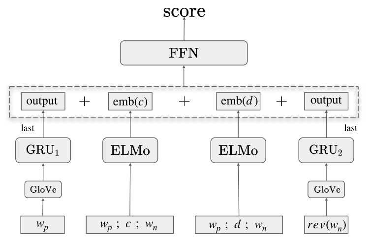
Figure 3.6: Illustration of the ELMo-based model $M_{\textit{ELMo}}$, where semicolon refers to vector concatenation.

We now describe models that are based on ELMo [8] which we denote $M_{\textit{ELMo}}$. Since MCDPara instances contain paragraph context, which usually includes more than one sentence, we denote the model that uses the full context by $M_{\textit{ELMo}}(\ell)$. By contrast, $M_{\textit{ELMo}}$ uses only a single sentence context for both MCDSent and MCDPara. We denote the correct answer by $c$, distractor candidate by $d$, the word sequence before the blank by $w_{p}$, and the word sequence after the blank by $w_{n}$, using the notation $\mathit{rev}(w_{n})$ to indicate the reverse of the sequence $w_{n}$.

We use GloVe [100] to obtain pretrained word embeddings for context words, then use two separate RNNs with gated recurrent units (GRUs; [101]) to output hidden vectors to represent $w_{p}$ and $w_{n}$. We reverse $w_{n}$ before passing it to its GRU, and we use the last hidden states of the GRUs as part of the classifier input. We also use ELMo to obtain contextualized word embeddings for correct answers and distractors in the given context, and concatenate them to the input. An illustration of this model is presented in Figure 3.6.

A feed-forward network (FFN) with 1 ReLU hidden layer is set on top of these features to get the score for classification:

$$\mathit{FFN}(z)=\max(0,zW_{1}+b_{1})W_{2}+b_{2}$$

where $z$ is a row vector representing the inputs shown in Figure 3.6. We train the model as a binary classifier by using a logistic sigmoid function on the output of $\mathit{FFN}(z)$ to compute the probability of the true label. Based on the model in Figure 3.6, we further experiment with the following variations of this model:

• Concatenate the features from Section 3.4 with $z$.

• Concatenate the correct answer to the input of the GRUs on both sides (denoted gru+c).

• Concatenate the GloVe embeddings of the correct answers and distractors with $z$. We combine this with gru+c, denoting the combination all.

3.5.3 BERT-Based Models

Our final model type uses a structure similar to $M_{\textit{ELMo}}$ but using BERT in place of ELMo when producing contextualized embeddings, which we denote by $M_{\textit{BERT}}$ and $M_{\textit{BERT}}(\ell)$ given different types of context. We also consider the variation of concatenating the features to the input to the classifier, i.e., the first variation described in Section 3.5.2. We omit the gru+c and all variations here because the BERT-based models are more computationally expensive than those that use ELMo.

3.6 Experiments

We now report the results of experiments with training models to select distractor candidates.

3.6.1 Evaluation Metrics

We use precision, recall, and F1 score as evaluation metrics. These require choosing a threshold for the score produced by our predictors. We also report the area under the precision-recall curve (AUPR), which is a single-number summary that does not require choosing a threshold.

3.6.2 Baselines

As the datasets are unbalanced (most distractor candidates are not selected), we report the results of baselines that always return “True” in the “baseline” rows of Tables 3.6 and 3.7. MCDSent has a higher percentage of true labels than MCDPara.

3.6.3 Estimates of Human Performance

dataset	precision		recall		F1
	A	B	A	B	A	B
MCDSent	62.9	48.5	59.5	43.2	61.1	45.7
MCDPara	32.1	25.0	36.0	24.0	34.0	24.5

Table 3.5: Results of human performance on distractor selection for two human judges labeled A and B.

We estimated human performance on the distractor selection task by obtaining annotations from NLP researchers who were not involved in the original data collection effort. We performed three rounds among two annotators, training them with some number of questions per round, showing the annotators the results after each round to let them calibrate their assessments, and then testing them using a final set of 30 questions, each of which has at most 10 distractors.

Human performance improved across rounds of training, leading to F1 scores in the range of 45-61% for MCDSent and 25-34% for MCDPara (Table 3.5). Some instances were very easy to reject, typically those that were erroneous word forms resulting from incorrect morphological inflection from the word form generator or those that were extremely similar in meaning to the correct answer. But distractors that were at neither extreme were very difficult to predict, as there is a certain amount of variability in the annotation of such cases. Nonetheless, we believe that the data has sufficient signal to train models to provide a score indicating suitability of candidates to serve as distractors.

3.6.4 Modeling and Training Settings

All models have one hidden layer for the feed-forward classifier. The $M_{\textit{feat}}$ classifier has 50 hidden units, and we train it for at most 30 epochs using Adam [102] with learning rate $1\mathrm{e}{-3}$. We stop training if AUPR keeps decreasing for 5 epochs. Although our primary metric of interest is AUPR, we also report optimal-threshold F1 scores on dev and test, tuning the threshold on the given set (so, on the test sets, the F1 scores we report are oracle F1 scores). The threshold is tuned within the range of 0.1 to 0.9 by step size 0.1.

For $M_{\textit{ELMo}}$ and $M_{\textit{ELMo}}(\ell)$, we use ELMo (Original) for the model, and BERT-large-cased to compute the BERT features from Section 3.4 (only applies to rows with “features = yes” in the tables). We increase the number of classifier hidden units to 1000 and run 20 epochs at most, also using Adam with learning rate $1\mathrm{e}{-3}$. We stop training if AUPR does not improve for 3 epochs.

For $M_{\textit{BERT}}$ and $M_{\textit{BERT}}(\ell)$, we applied the same training settings as $M_{\textit{ELMo}}$ and $M_{\textit{ELMo}}(\ell)$. We compare the BERT-base-cased and BERT-large-cased variants of BERT. When doing so, the BERT features from Section 3.4 use the same BERT variant as that used for contextualized word embeddings.

For all models based on pretrained models, we keep the parameters of the pretrained models fixed. However, we do a weighted summation of the 3 layers of ELMo, and all layers of BERT except for the first layer, where the weights are trained during the training process.

3.6.5 Results

model	variant	development set				test set				BERT	features	best	threshold
		precision	recall	F1	AUPR	precision	recall	F1	AUPR			epoch
baseline		15.4	100	26.7	-	13.3	100	23.5	-	-	-	-	-
		33.6	62.9	43.8	36.5	23.7	55.4	33.2	24.6	none	yes	28	0.2
$M_{\textit{feat}}$		44.5	57.1	50.0	46.1	28.2	70.9	40.3	32.4	base	yes	25	0.2 (0.3)
		36.4	77.8	49.6	47.0	30.0	71.3	42.2	34.5	large	yes	22	0.2
	none	43.2	87.5	57.8	59.0	41.4	88.0	56.3	54.6	-	no	2	0.3
	gru+c	44.8	84.4	58.5	57.4	47.6	68.4	56.1	54.1	-	no	2	0.3 (0.4)
$M_{\textit{ELMo}}$	all	47.2	88.9	61.7	61.2	48.3	75.0	58.7	55.8	-	no	2	0.3 (0.4)
	none	51.7	77.8	62.1	64.6	50.4	76.5	60.8	57.2	large	yes	3	0.3
	gru+c	55.7	73.3	63.3	65.3	49.1	82.3	61.5	63.1	large	yes	5	0.4 (0.3)
	all	56.2	74.4	64.0	66.5	49.8	80.8	61.6	58.8	large	yes	5	0.4 (0.3)
		47.9	78.1	59.4	60.8	44.8	81.0	57.7	55.7	base	no	1	0.3
$M_{\textit{BERT}}$		49.6	79.3	61.0	64.1	45.3	80.2	57.9	53.4	large	no	1	0.3
		50.6	83.9	63.2	65.3	44.8	78.5	57.0	53.8	base	yes	12	0.1
		53.8	73.1	62.0	66.5	49.7	73.9	59.4	56.3	large	yes	2	0.4

Table 3.6: Results for MCDSent. Boldface indicates the best F1/AUPR on dev/test for each model type. We include the threshold tuned on the test set in parentheses when it differs from the threshold tuned on dev.

model	development set				test set				BERT	features	best epoch	threshold
	precision	recall	F1	AUPR	precision	recall	F1	AUPR
baseline	7.3	100	13.5	-	6.6	100	12.4	-	-	-	-	-
	15.3	63.1	24.6	17.3	14.5	63.6	23.6	15.5	-	yes	23	0.1
$M_{\textit{feat}}$	18.2	69.2	28.9	21.6	16.3	65.6	26.1	19.1	base	yes	27	0.1
	19.8	64.0	30.2	22.3	16.9	64.2	26.8	18.8	large	yes	22	0.1
$M_{\textit{ELMo}}$	35.4	47.7	40.7	38.4	26.1	75.6	38.8	30.4	-	no	5	0.3 (0.2)
	37.9	61.3	46.9	46.8	34.6	63.9	44.9	37.6	large	yes	7	0.3
$M_{\textit{ELMo}}(\ell)$	30.5	61.1	40.7	36.6	29.1	61.6	39.5	33.2	-	no	5	0.3
	37.1	62.7	46.6	43.7	34.4	65.1	45.0	40.1	large	yes	6	0.3
	35.4	61.6	45.0	40.9	29.2	58.7	39.0	30.1	base	no	2	0.2
$M_{\textit{BERT}}$	33.0	63.7	43.5	40.9	29.1	65.1	40.2	32.4	large	no	2	0.2
	44.3	55.4	49.3	47.3	31.5	73.2	44.0	36.7	base	yes	2	0.3 (0.2)
	35.6	66.0	46.2	45.0	35.5	54.5	43.0	36.6	large	yes	2	0.2 (0.3)
$M_{\textit{BERT}}(\ell)$	33.1	65.3	43.9	39.7	28.8	66.4	40.2	29.8	base	no	2	0.2
	37.4	67.3	48.1	46.0	31.3	69.1	43.1	37.0	base	yes	2	0.2

Table 3.7: Results for MCDPara (tuned based on AUPR).

We present our main results for MCDSent in Table 3.6 and for MCDPara in Table 3.7.

Feature-based models.

The feature-based model, shown as $M_{\textit{feat}}$ in the upper parts of the tables, is much better than the trivial baseline. Including the BERT features in $M_{\textit{feat}}$ improves performance greatly (10 points in AUPR for MCDSent), showing the value of using the context effectively with a powerful pretrained model. There is not a large difference between using BERT-base and BERT-large when computing these features.

ELMo-based models.

Even without features, $M_{\textit{ELMo}}$ outperforms $M_{\textit{feat}}$ by a wide margin. Adding features to $M_{\textit{ELMo}}$ further improves F1 by 2-5% for MCDSent and 5-6% for MCDPara. The F1 score for $M_{\textit{ELMo}}$ on MCDSent is close to human performance, and on MCDPara the F1 score outperforms humans (see Table 3.5). For MCDSent, we also experiment with using the correct answer as input to the context GRUs (gru+c), and additionally concatenating the GloVe embeddings of the correct answers and distractors to the input of the classifier (all). Both changes improve F1 on dev, but on test the results are more mixed.

BERT-based models.

For $M_{\textit{BERT}}$, using BERT-base is sufficient to obtain strong results on this task and is also cheaper computationally than BERT-large. Although $M_{\textit{BERT}}$ with BERT-base has higher AUPR on dev, its test performance is close to $M_{\textit{ELMo}}$. Adding features improves performance for MCDPara (3-5% F1), but less than the improvement found for $M_{\textit{ELMo}}$. While $M_{\textit{feat}}$ is aided greatly when including BERT features, the features have limited impact on $M_{\textit{BERT}}$, presumably because it already incorporates BERT in its model.

Long-context models.

We now discuss results for the models that use the full context in MCDPara, i.e., $M_{\textit{ELMo}}(\ell)$ and $M_{\textit{BERT}}(\ell)$. On dev, $M_{\textit{ELMo}}$ and $M_{\textit{BERT}}$ outperform $M_{\textit{ELMo}}(\ell)$ and $M_{\textit{BERT}}(\ell)$ respectively, which suggests that the extra context for MCDPara is not helpful. However, the test AUPR results are better when using the longer context, suggesting that the extra context may be helpful for generalization. Nonetheless, the overall differences are small, suggesting that either the longer context is not important for this task or that our way of encoding the context is not helpful. The judges in our manual study (Sec. 3.6.3) rarely found the longer context helpful for the task, pointing toward the former possibility.

3.6.6 Statistical Significance Tests

For better comparison of these models’ performances, a paired bootstrap resampling method is applied [103]. We repeatedly sample with replacement 1000 times from the original test set with sample size equal to the corresponding test set size, and compare the F1 scores of two models. We use the thresholds tuned by the development set for F1 score computations, and assume significance at a $p$ value of 0.05.

• For $M_{\textit{ELMo}}$, $M_{\textit{ELMo}}(\ell)$, $M_{\textit{BERT}}$ and $M_{\textit{BERT}}(\ell)$, the models with features are significantly better than their feature-less counterparts ($p<0.01$).

• When both models use features, $M_{\textit{ELMo}}(\ell)$ is almost the same as $M_{\textit{ELMo}}$ ($p=0.477$). However, when both do not use features, $M_{\textit{ELMo}}(\ell)$ is significantly better ($p<0.01$).

• When using BERT-base-cased, $M_{\textit{BERT}}(\ell)$ is better than $M_{\textit{BERT}}$, but not significantly so ($p=0.4$ with features and $0.173$ without features).

• On MCDPara, switching from BERT-base to BERT-large does not lead to a significant difference for $M_{\textit{BERT}}$ without features (BERT-large is better with $p=0.194$) or $M_{\textit{BERT}}$ with features (BERT-base is better with $p=0.504$). For MCDSent, $M_{\textit{BERT}}$ with BERT-large is better both with and without features ($p<0.2$).

• On MCDPara, $M_{\textit{BERT}}(\ell)$ outperforms $M_{\textit{ELMo}}(\ell)$ without features but not significantly. With features, $M_{\textit{ELMo}}(\ell)$ is better with $p=0.052$.

• On MCDSent, $M_{\textit{BERT}}$ without features (BERT-large-cased) is better than $M_{\textit{ELMo}}$ without features, but not significantly so ($p=0.386$). However, if we add features or use $M_{\textit{BERT}}$ with BERT-base-cased, $M_{\textit{ELMo}}$ is significantly better ($p<0.01$).

• On MCDPara, $M_{\textit{ELMo}}$ is nearly significantly better than $M_{\textit{BERT}}$ when both use features ($p=0.062$). However, dropping the features for both models makes $M_{\textit{BERT}}$ significantly outperform $M_{\textit{ELMo}}$ ($p=0.044$).

3.6.7 Examples

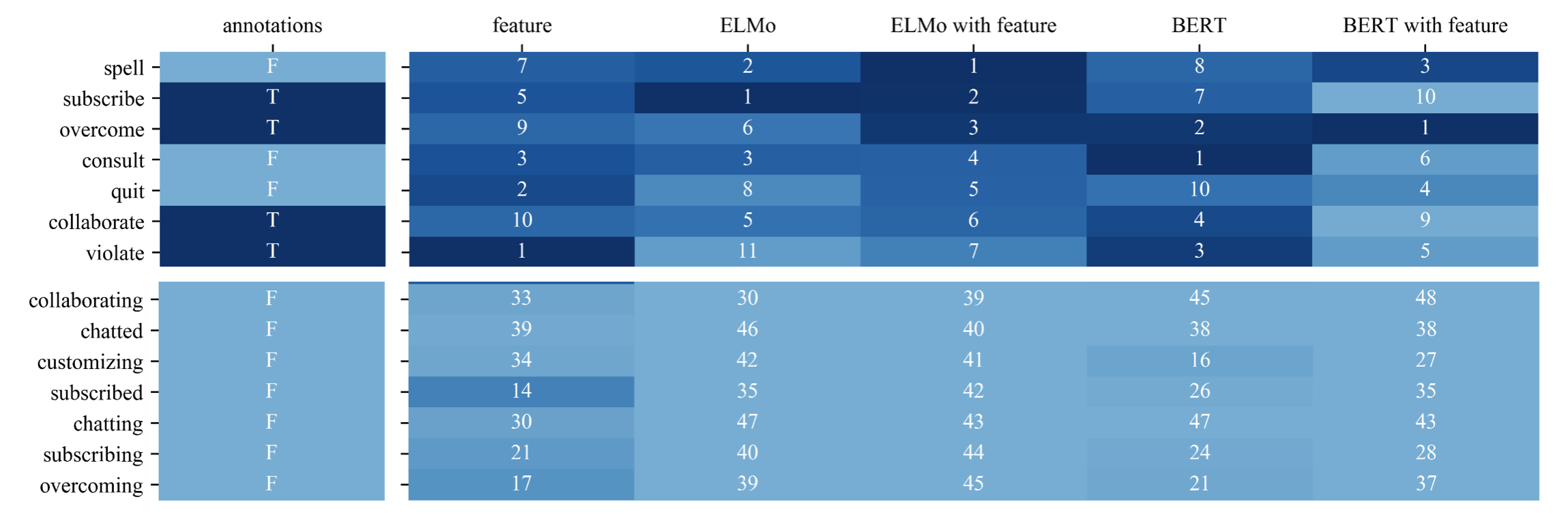
Figure 3.7: Ranks of distractors for question “The bank will notify its customers of the new policy.” The colors represent the normalized scores of the models and the numbers in the cells are the ranks of the candidates.

Figure 3.7 shows an example question from MCDSent, i.e., “The bank will notify its customers of the new policy”, and two subsets of its distractors. The first subset consists of the top seven distractors using scores from $M_{\textit{ELMo}}$ with features, and the second contains distractors further down in the ranked list. For each model, we normalize its distractor scores with min-max normalization.

Overall, model rankings are similar across models, with all distractors in the first set ranked higher than those in the second set. The high-ranking but unselected distractors (“spell”, “consult”, and “quit”) are likely to be reasonable distractors for second-language learners, even though they were not selected by annotators.

We could observe the clustering of distractor ranks with similar morphological inflected form in some cases, which may indicate that the model makes use of the grammatical knowledge of pretrained models.

3.7 Conclusion

We described two datasets with annotations of distractor selection for multiple-choice cloze questions for second-language learners. We designed features and developed models based on pretrained language models. Our results show that the task is challenging for humans and that the strongest models are able to approach or exceed human performance. The rankings of distractors provided by our models appear reasonable and can reduce a great deal of human burden in distractor selection. Future work will use our models to collect additional training data which can then be refined in a second pass by limited human annotation. Other future work can explore the utility of features derived from pretrained question answering models in scoring distractors.

Chapter 4 The Benefits of Label-Description Training for Zero-Shot Text Classification

In this chapter, we examine the challenge of zero-shot text classification. This task requires the model to generalize from its existing knowledge without any labeled data for the new classes. Recent approaches transform text classification into a language modeling task [18]. However, this method is highly sensitive to the prompt design and the specific words or phrases used to represent the labels.

Since the model must have a deep understanding of both the text and the class labels to achieve good performance, we propose to finetune the pretrained language model with a small curated dataset of label descriptions, which improves both model performance and robustness.

This chapter is based on [37].

4.1 Introduction

Pretrained language models (PLMs) [104, 10, 20, 17, 105] have produced strong results in zero-shot text classification for a range of topic and sentiment tasks, often using a pattern-verbalizer approach [18]. With this approach, to classify the restaurant review “Overpriced, salty and overrated!”, a pattern like “the restaurant is [MASK]” is appended to the review and verbalizers are chosen for each label (e.g., “good” for positive sentiment and “bad” for negative). The text is classified by the pretrained masked language modeling (MLM) head to choose the most probable verbalizer for the [MASK] position. Although effective, the approach is sensitive to the choice of specific pattern/verbalizer pairs, with subtle changes in the pattern, the verbalizer, or both, often having a large impact on performance [24, 23].

Label	Input
Business	business
	finance
	Business is the activity of making one’s living or making money by producing or buying and selling products…
Sports	sports
	racing
	An athletic activity requiring skill or physical prowess and often of a competitive nature, as racing, baseball, tennis, golf,…

(a) Topic classification

Label	Input
Very Negative	awful
	It was terrible.
	A horrendous experience.
Very Positive	great
	Just fantastic.
	Overall, it was outstanding.

(b) Sentiment classification

Table 4.1: A few examples of LabelDesc training data for topic and sentiment classification.

To alleviate these issues, we propose a simple alternative approach of training on small curated datasets intended to describe the labels for a task. Unlike typical training datasets, which consist of input texts annotated by hand with labels, our data contains only the descriptions of the labels. We refer to this data as LabelDesc data and show a few examples for topic and sentiment classification in Table 4.1. For topic classification, we include a few terms related to the label (e.g., “finance” for “Business”, “racing” for “Sports”), a definition of the label from dictionary.com (e.g., “An athletic activity …” for “Sports”), and a sentence from the opening paragraph of the label’s Wikipedia article (e.g., “Business is the activity of …” for “Business”). For sentiment classification, we simply use related terms that capture the specific sentiment (e.g., “terrible” for “Very Negative”) as well as a few hand-crafted templates (e.g., “It was $t$.” where $t$ is a related term).

Next, we finetune pretrained models using the pattern-verbalizer approach on LabelDesc data and evaluate them for text classification. For topic classification, we use patterns and verbalizers from Schick and Schütze [106] to train on our LabelDesc examples by finetuning the model as well as the MLM head (see Section 4.4 for details). We refer to training on LabelDesc data as LabelDescTraining. In experiments, we show that LabelDescTraining consistently improves accuracy (average improvement of 17-19%) over zero-shot classification across multiple topic and sentiment datasets (Table 4.9). We also show that LabelDescTraining can decrease accuracy variance across patterns compared to zero-shot classification (Table 4.10), thus being less sensitive to the choice of pattern.

We then conduct additional experiments to reveal the value of LabelDescTraining under various circumstances. To study the impact of verbalizer choice, we experiment with uninformative (randomly initialized) and adversarial (intentionally mismatched) verbalizers (Section 4.6.1). While accuracy drops slightly, both settings are still much more accurate than zero-shot classification with its original verbalizers. That is, LabelDescTraining is able to compensate for knowledge-free or even adversarial verbalizer choice. We also compare to finetuning a randomly initialized classifier head without any patterns or verbalizers, again finding accuracy to be higher than zero-shot (Section 4.6.2). Collectively, our results demonstrate that LabelDescTraining leads to strong performance that is less sensitive than zero-shot classification in terms of pattern/verbalizer choice, while also not requiring a pretrained MLM head.

Since LabelDesc data focuses entirely on the labels without seeking to capture the input text distribution, we would hope that it would exhibit stable performance across datasets with the same labels. So, we compare LabelDescTraining to the approach of training on a small supervised training set from one domain and testing on another (Section 4.6.4). In multiple cases, LabelDescTraining actually attains higher accuracy than few-shot supervised learning tested on out-of-domain test sets, even when hundreds of manually labeled training examples are used (albeit from a different input domain).

In summary, this paper shows several benefits of LabelDescTraining. First, once a practitioner identifies a label set of interest for zero-shot classification, it only requires a few minutes to collect the kind of LabelDesc data shown in Table 4.1, and training on this data improves over zero-shot by 17-19% absolute. Second, LabelDescTraining leads to greater robustness to pattern/verbalizer choice than zero-shot. Third, LabelDesc data are domain independent with regard to the distribution of the inputs; a single LabelDesc training set can be used for any text classification task as long as it contains the same labels. Our experiments show that this independence to input distribution leads to stable accuracy across domains, even attaining higher accuracy than out-of-domain few-shot learning on a few cases.

4.2 Related Work

One common approach in zero-shot text classification is to transfer knowledge from seen labels [107], which requires observed labels and a notion of label similarity. Some sources of semantic knowledge used for this purpose include multiple modalities [108], label relationships in knowledge graphs [109], and word representations [110, 111].

There are several other approaches to zero-shot classification. To classify documents, Chang et al. [112] used knowledge-based text representations derived from Wikipedia, and Barak et al. [113] used both Wikipedia and WordNet. However, they both require a large-scale knowledge base. Zhang et al. [114] combined label descriptions with a label hierarchy and word-to-label paths in ConceptNet, with data augmentation strategies. Yin et al. [115] used a textual entailment approach with label definitions from WordNet. Another approach that has gained popularity is self-training given label names and acquiring knowledge by mining an unlabeled dataset [116, 117]. van de Kar et al. [24] extend the mining-based approach by selecting unsupervised examples (via patterns) for training. Basile et al. [118] select label descriptions by aggregation. Meng et al. [119] use language models to generate new training examples. On the contrary, we train on a small set of domain-independent label descriptions. Our setup is influenced by Schick and Schütze [18, 106], although, instead of finetuning on training examples, we only use our LabelDesc data.

Autoregressive language models have also been used for zero-shot text classification; we report zero-shot and ICL results with LabelDesc data using GPT-3.5 [53]. Zhao et al. [120] found it beneficial to “calibrate” such models for this setting; this idea is not immediately applicable here due to our use of encoder-only models like RoBERTa. Calibration could be extended to encoder-only models, which we plan to explore in future work. Our work is closely related to dataless classification [112] which involves building classifiers by designing or learning a generic function that scores the compatibility of a document and label defined in natural language. We compared empirically to the dataless classification approaches of Chu et al. [121] and Chu et al. [122] who used pretrained models, naturally annotated data like that from Wikipedia categories, and unsupervised clustering techniques. There is a wealth of prior work in semi-supervised text classification [123, 124, 125]. There is also related work on generating label names [126] or label descriptions [127, 128] but for supervised text classification.

4.3 Tasks and LabelDesc Datasets

We evaluate on two types of tasks: topic classification on AGNews, Yahoo Answers, and DBPedia [1] and sentiment classification on the Stanford Sentiment Treebank (SST) [129], Yelp Reviews [1], IMDB [130], and Amazon Reviews Polarity [1]. We consider both binary and 5-way classification for SST and Yelp datasets (denoted as SST-2, SST-5, Yelp-2, and Yelp-5 henceforth) and only binary for IMDB and Amazon (denoted as IMDB and Amz-2 henceforth). Dataset statistics are in Table 4.2. Below we describe how we construct LabelDesc data for each label set.

dataset	#label	LD	dev	test
20NG	4	24	3389	-
AGNews	4	24	2,000	7,600
Yahoo${}_{\textrm{AG}}$			3,000	36,000
Yahoo	10	60	-	60,000
DBPedia	14	84	-	70,000
Yelp-5	5	125	2,500	50,000
SST-5			1,101	2,210
Yelp-2	2	100	2,000	38,000
SST-2			872	1,821
Amz-2			-	400,000
IMDB			-	25,000

Table 4.2: Statistics of datasets we used, with ’#’ denoting the number of labels, LD refers to LabelDesc data.

4.3.1 Topic Classification

Since labels in topic classification represent general concepts, we use both subjective descriptors of the labels (e.g., related terms) and objective sources of information (e.g., dictionary definition and Wikipedia sentences) when selecting LabelDesc data. In particular, we create LabelDesc examples for the label term itself, three related terms, a selected definition from dictionary.com, and the leading sentence from the label’s Wikipedia article. As there are typically multiple dictionary.com definitions for our labels, we select a single definition that best aligns with our understanding of the concept underlying the label. We use the leading Wikipedia sentence because it is typically a brief overview/definition of the concept. Most labels in the Yahoo dataset consist of two keywords (e.g., Society & Culture). For these, we use both label terms, definitions for each, and the leading Wikipedia sentences for each. As an example, the LabelDesc data for AGNews is shown in Table 4.3.

Label	Type	Training Data
World	terms	world | country | international | politics
	Wiki.	In its most general sense, the term “world” refers to the totality of entities, to the whole of reality or to everything that is.
	dict.	humankind; the human race; humanity
Sports	terms	sport | sports | racing | baseball
	Wiki.	Sport pertains to any form of competitive physical activity or game that aims to use, maintain or improve physical ability and skills while providing enjoyment to participants and, in some cases, entertainment to spectators.
	dict.	an athletic activity requiring skill or physical prowess and often of a competitive nature, as racing, baseball, tennis, golf, bowling, wrestling, boxing, hunting, fishing, etc.
Business	terms	business | finance | money | trade
	Wiki.	Business is the activity of making one’s living or making money by producing or buying and selling products (such as goods and services).
	dict.	the purchase and sale of goods in an attempt to make a profit.
Sci/Tech	terms	technology | science | computer | biology
	Wiki.	Technology is the continually developing result of accumulated knowledge and application in all techniques, skills, methods, and processes used in industrial production and scientific research.
	dict.	the branch of knowledge that deals with the creation and use of technical means and their interrelation with life, society, and the environment, drawing upon such subjects as industrial arts, engineering, applied science, and pure science.

Table 4.3: LabelDesc data for AGNews (and Yahoo${}_{\textrm{AG}}$).

We did not tune any of these decisions experimentally, so these choices in defining LabelDesc data are almost certainly suboptimal. This suboptimality is especially likely for the “World” label in the AGNews label set. This label reflects international news, but the dictionary definition and Wikipedia article for the term “World” do not capture that sense of the word. Nonetheless, we did not change our procedure for this label because we wanted our results to reflect a real-world implementation of the idea, complete with its limitations for certain labels.

The LabelDesc instances we are using do not contain exhaustive information. We could easily extend the lists of related terms for each topic or use WordNet or other semantic knowledge resources [114]. However, one of the goals of this research is to demonstrate how simple it is to choose LabelDesc examples to improve zero-shot classification in very little time.

4.3.2 Sentiment Classification

We use a slightly different procedure for sentiment classification. For 5-way sentiment, we use the label verbalizer itself and four synonym terms. In addition, we write four simple templates: “It was $t$.”, “A(n) $t$ experience.”, “Just $t$.”, and “Overall, it was $t$.”, where $t$ is the label verbalizer or a synonym. For binary sentiment, we remove the neutral instances, combine the two positive labels (“Very Positive” and “Positive”) into one, and combine the two negative labels (“Very Negative” and “Negative”) into one. This procedure produces a total of 25 examples per label (5 terms + 5 terms $\times$ 4 templates) for 5-way sentiment and 50 examples per label for binary sentiment. Since these LabelDesc instances are domain-independent, we use the same data for both for 5-way sentiment (Yelp-5 and SST-5) and for binary sentiment (Yelp-2, SST-2, IMDB-2, Amz-2). As an example, the LabelDesc data for Yelp-5 and SST-5 is shown in Table 4.4.

Label	Type	Training Data
Very Negative	terms	awful | terrible | horrendous | horrible | dreadful
	sent.	It was $t$. | A(n) $t$ experience. | Just $t$. | Overall, it was $t$.
Negative	terms	bad | unpleasant | unsatisfying | lousy | subpar
	sent.	It was $t$. | A(n) $t$ experience. | Just $t$. | Overall, it was $t$.
Neutral	terms	okay | mediocre | decent | average | alright
	sent.	It was $t$. | A(n) $t$ experience. | Just $t$. | Overall, it was $t$.
Positive	terms	good | nice | fine | pleasant | neat
	sent.	It was $t$. | A(n) $t$ experience. | Just $t$. | Overall, it was $t$.
Very Positive	terms	great | amazing | excellent | fantastic | outstanding
	sent.	It was $t$. | A(n) $t$ experience. | Just $t$. | Overall, it was $t$.

Table 4.4: LabelDesc data for Yelp-5 and SST-5. “Sent.” and “$t$” refer to hand-crafted sentence templates and terms, respectively.

4.3.3 Hyperparameter Tuning

We adhere to the “true” zero-shot setting where hyperparameters cannot be tuned on a development set for the task of interest [106]. Therefore, we use a separate dataset for hyperparameter tuning - the 20 Newsgroups (20NG, henceforth) [131] - a topic classification dataset with twenty labels. We select only four labels from 20NG for our purposes: talk.religion.misc, rec.autos, sci.med, and talk.politics.guns. We chose these four labels because they are sufficiently distinct that we expect tuning to be informative for other real-world classification datasets; many of the other 20NG labels are highly technical or similar to one other, e.g., the pair comp.sys.ibm.pc.hardware and comp.sys.mac.hardware as well as the pair comp.os.ms-windows.misc and comp.windows.x. We follow the same strategy as for topic classification above when constructing LabelDesc data for 20NG. The selected hyperparameters are used for both topic and sentiment classifications.

4.4 Experimental Settings

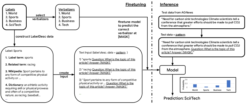
Figure 4.1: Overview of our proposed method, including the construction of LabelDesc data, the format of the text input, and the target used for both model finetuning and inference during test time. We present text inputs labeled as “Sports” from the topic classification task, and use one of our patterns (see Table 4.6) here as an illustration. Note that all our LabelDesc datasets are balanced, with each pattern being associated with a unique finetuned model checkpoint.

The following settings are used in our experiments. Unless stated otherwise, we use the pretrained RoBERTa-base ($b$) and RoBERTa-large ($l$) models [20] for all experiments since RoBERTa is the predominant choice in related zero-shot and dataless research [18, 24, 117]. Additionally, for every dataset, we use the entire available test sets for evaluation.

4.4.1 Patterns and Verbalizers

Dataset	Verbalizers
20NG	talk.religion.misc $\mapsto$ religion, rec.autos $\mapsto$ automobile, sci.med $\mapsto$ medicine, talk.politics.guns $\mapsto$ gun
AGNews	World $\mapsto$ World, Sports $\mapsto$ Sports, Business $\mapsto$ Business, Sci/Tech $\mapsto$ Tech
Yahoo	Society & Culture $\mapsto$ Society, Science & Mathematics $\mapsto$ Science, Health $\mapsto$ Health, Education & Reference $\mapsto$ Education, Computers & Internet $\mapsto$ Computer, Sports $\mapsto$ Sports, Business & Finance $\mapsto$ Business, Entertainment & Music $\mapsto$ Entertainment, Family & Relationships $\mapsto$ Relationship, Politics & Government $\mapsto$ Politics
DBPedia	Company $\mapsto$ company, Educational institution $\mapsto$ school, Artist $\mapsto$ artist, Athlete $\mapsto$ sports, Office holder $\mapsto$ politics, Mean of transportation $\mapsto$ transportation, Building $\mapsto$ building, Natural place $\mapsto$ natural, Village $\mapsto$ village, Animal $\mapsto$ animal, Plant $\mapsto$ plant, Album $\mapsto$ album, Film $\mapsto$ film, Written work $\mapsto$ book
Yelp-5	Very Negative $\mapsto$ terrible, Negative $\mapsto$ bad, Neutral $\mapsto$ okay, Positive $\mapsto$ good, Very Positive $\mapsto$ great
SST-5
Yelp-2	Negative $\mapsto$ awful, Positive $\mapsto$ great
SST-2
IMDB
Amz-2

Table 4.5: Verbalizers selected for each dataset.

4.4.2 Zero-shot Classification Baseline

type	id	patterns
Q&A	1	$x$ Question: What is the topic of this article? Answer: [MASK].
	2	$x$ Question: What is the category of this article? Answer: [MASK].
	3	$x$ Question: What is the topic of this article? Answer: [MASK]
	4	$x$ Question: What is the category of this article? Answer: [MASK]
Prompt	1	$x$ Category: [MASK].
	2	$x$ Class: [MASK].
	3	$x$ Topic: [MASK].
	4	$x$ Theme: [MASK].
	5	$x$ Category: [MASK]
	6	$x$ Class: [MASK]
	7	$x$ Topic: [MASK]
	8	$x$ Theme: [MASK]
	9	[MASK] News: $x$
	10	[MASK] NEWS: $x$

(a) Patterns for AGNews

type	id	patterns
Q&A	1	$x$ Question: What is the sentiment of this text? Answer: [MASK].
	2	$x$ Question: What is the writer’s opinion in this text? Answer: [MASK].
	3	$x$ Question: What is the sentiment of this text? Answer: [MASK]
	4	$x$ Question: What is the writer’s opinion in this text? Answer: [MASK]
Prompt	1	$x$ Opinion: [MASK].
	2	$x$ Feeling: [MASK].
	3	$x$ Sentiment: [MASK].
	4	$x$ Summary: [MASK].
	5	$x$ Opinion: [MASK]
	6	$x$ Feeling: [MASK]
	7	$x$ Sentiment: [MASK]
	8	$x$ Summary: [MASK]
	9	[MASK] Sentiment: $x$
	10	[MASK] SENTIMENT: $x$

(b) Patterns for sentiment classification

Table 4.6: Patterns where $x$ refers to the given text.

We use the standard “pattern-verbalizer” approach for topic and sentiment classification. The set of verbalizers used can be found in Table 4.5. For choosing verbalizers, we follow the choices of Schick and Schütze [18] for AGNews, Yahoo, Yelp-5, and SST-5. We follow van de Kar et al. [24] in choosing verbalizers for Yelp-2, SST-2, IMDB, and Amz-2 and we select verbalizers for DBPedia and 20NG ourselves.

Each pattern comprises a prompt including a [MASK] symbol placed before or after the text input, and we aim to predict the masked token. For example, a prompt is added after the input $x$ to frame classification as a question answering task, e.g., “$x$ Question: What is the topic of this newsgroup? Answer: [MASK].” We use RoBERTa-base/large with its MLM head for zero-shot experiments. Although the model is able to predict any token within its vocabulary, we choose only among the set of verbalizers, which are designed to be semantically coherent with class labels and tokenized into a single token by the model’s tokenizer.

For 20NG, we remove headers, quotes, and footers. For AGNews, we concatenate the headlines and the text body of the news articles. For Yahoo dataset, we concatenate the title, the question, and the top answer to it. And for IMDB and Amazon Reviews Polarity datasets, we concatenate the title and the content.

For topic classification tasks, we use the Prompt and Q&A patterns from Schick and Schütze [106], which amounts to 14 patterns. For AGNews, we use “news/article” in the pattern templates, while for Yahoo we replace this with “question”, and for 20NG we use “newsgroup”. The patterns are shown in Table 4.6 (a). For the sentiment classification tasks, we create new Q&A patterns such as “$x$ Question: What is the sentiment of this text? Answer: [MASK].” and Prompt patterns such as “$x$ Sentiment: [MASK].” where $x$ is the input text. There are 14 sentiment patterns in total shown in Table 4.6 (b).

4.4.3 LabelDescTraining

We use the same settings as the zero-shot baseline except that we finetune the models on LabelDesc data. We do not use any target task data for tuning or early stopping. Instead, we fix hyperparameter values, including number of training steps, by tuning on 20NG following the process described below.

We used LabelDesc data for the four selected 20NG labels as our training data and the original 20NG data (training and test sets) as our dev set, restricted to the four selected labels shown in Section 4.3. We preprocessed the data by removing headers, quotes, and footers. We used a batch size of 1 and tuned over a set of five learning rates ({5e-7, 1e-6, 5e-6, 1e-5, 5e-5}). Models were trained for 3500 training steps, evaluating on the dev set after each epoch, i.e., every 24 training steps since it’s the size of LabelDesc dataset for 20NG.

			lr	steps
MLM	LDT	base	5e-7	2160
		large	5e-7	1920
	mismatched	base	5e-5	2160
		large	5e-6	3000
	random	base	5e-5	2160
		large	5e-6	3240
classifier	base		1e-5	1920
	large		1e-6	2280

Table 4.7: Hyperparameters (learning rate, training steps) selected by tuning on 20NG with RoBERTa.

			pattern	id
MLM	LDT	base	prompt	9
		large	prompt	7
	mismatched	base	qa	3
		large	qa	1
	random	base	qa	3
		large	prompt	6

Table 4.8: Tuned pattern and pattern id for each model.

After fine-tuning on 20NG, the hyperparameters are selected as shown in Table 4.7. The tuned patterns are listed in Table 4.8. To our knowledge, this method works well when we adapt to other datasets. However, we also observe that there are fluctuations in the dev accuracy curve for 20NG during training, and we select the training steps in the middle of the flatter part of curves rather than the peak point for robustness. We suggest changing training steps or increasing batch size if this method doesn’t work well. The tuned pattern is not necessarily the best pattern after adapting to other datasets, sometimes even a little lower than the average results over all 14 patterns.

Based on tuning accuracies, we chose learning rate 5e-7 and number of training steps 2160 for RoBERTa-base and 1920 for RoBERTa-large. Additionally, we explored variations of parameter freezing, such as freezing certain layers of RoBERTa. The best setting on 20NG was to freeze the lower half of the layers (excluding the embedding layer) during finetuning, so we used this for experiments reported below.

4.5 Results

Table 4.9 compares standard zero-shot classification and LabelDescTraining. LabelDescTraining has higher accuracy across all topic and sentiment classification datasets, outperforming zero-shot by about 17% on average when using RoBERTa-base and 19% with RoBERTa-large. The results demonstrate that we can greatly improve the performance of zero-shot models with just a few training examples that provide a richer characterization of the label but still without requiring any textual inputs from the task datasets.

		AGNews	Yahoo	DBPedia	Yelp-5	SST-5	Yelp-2	SST-2	Amz-2	IMDB	Avg.
zero-shot	$b$	62.7	41.5	54.6	38.0	35.6	63.6	62.6	64.0	69.9	54.7
	$l$	68.0	47.7	63.9	38.7	35.0	70.6	63.7	67.5	74.1	58.8
LabelDescTraining	$b$	77.4	58.8	79.5	43.6	42.0	88.3	84.5	88.6	86.9	72.2
	$l$	79.4	60.8	86.6	51.3	49.2	94.6	91.3	94.1	92.1	77.7

Table 4.9: Test accuracy (%) comparison between zero-shot classification and LabelDescTraining, b = RoBERTa-base, l = RoBERTa-large. For zero-shot, each result is the average over 14 patterns; and for LabelDescTraining, each result is the average over 14 patterns and three random seeds per pattern. The “Avg.” column shows the average accuracies across columns.

		AGNews	Yahoo	DBPedia	Yelp-5	SST-5	Yelp-2	SST-2	Amz-2	IMDB
zero-shot	$b$	7.4	7.0	18.9	4.3	4.3	10.7	11.0	10.3	13.2
	$l$	7.8	8.2	9.7	7.8	7.7	15.7	14.3	13.7	17.0
LDT	$b$	5.0, 5.1, 5.0	1.7, 1.6, 1.6	4.5, 4.5, 4.5	2.0, 2.1, 2.2	1.8, 1.4, 1.5	2.1, 2.8, 2.4	2.5, 2.3, 1.9	1.3, 1.2, 1.4	1.8, 2.3, 1.4
	$l$	5.3, 6.4, 4.6	2.1, 2.0, 2.3	3.2, 2.9, 3.2	2.4, 2.5, 2.4	1.6, 1.2, 1.5	1.1, 2.5, 1.4	1.2, 2.8, 1.6	0.9, 1.9, 0.8	1.1, 1.4, 1.2

Table 4.10: Standard deviations of test accuracy (%) across 14 patterns for each test dataset. For LabelDescTraining (LDT in the table), three random seeds were used so we show three standard deviations, one per random seed. All standard deviations over patterns are smaller for LDT than the corresponding values for zero-shot.

		AGNews	Yahoo	DBPedia	Yelp-5	Yelp-2	SST-5	SST-2	Amz-2	IMDB
LabelDescTraining	$b$	84.6$\pm$0.3	59.9$\pm$0.3	82.4$\pm$1.2	42.0$\pm$0.4	84.8$\pm$0.6	44.3$\pm$0.1	88.2$\pm$0.2	89.6$\pm$0.4	83.4$\pm$0.4
	$l$	85.1$\pm$1.0	61.2$\pm$0.3	88.5$\pm$0.4	52.5$\pm$1.2	95.3$\pm$0.4	49.4$\pm$1.1	91.4$\pm$0.8	94.5$\pm$0.3	92.9$\pm$0.1
Chu et al. [121]	$b$	68.8	57.8	81.9	-	67.3	-	65.0	66.8	-
Chu et al. [122]	$b$	75.1	60.0	88.6	-	-	-	-	-	-
Schick and Schütze [106]	10	79.5$\pm$2.2	58.4$\pm$2.7	-	44.3$\pm$2.5	-	-	-	-	-
	100	87.5$\pm$0.8	65.3$\pm$1.0	-	54.8$\pm$1.5	-	-	-	-	-
van de Kar et al. [24]	$b$	79.2	56.1	80.4	-	92.0	-	85.6	92.0	86.7

Table 4.11: Test accuracy (%) comparison to state-of-the-art methods. 10/100 = # labeled examples used.

Table 4.10 shows that accuracy variances across patterns using LabelDescTraining are much lower than the zero-shot setting, which is known to be unstable [23]. Finetuning on LabelDesc data not only improves accuracy, but also mitigates sensitivity to pattern selection.

4.5.1 Comparisons to the State of the Art

We compare to state-of-the-art (SOTA) results from the literature in Table 4.11 (we show results using RoBERTa-base to better compare to other methods). For this comparison, we use only a single pattern with LabelDescTraining, since doing so reflects more of a real-world use case than averaging over 14 patterns. We choose a single pattern for each of RoBERTa-base and large by tuning on 20NG as we did for other hyperparameters. We use three random seeds and report average accuracies and standard deviations over seeds.

Chu et al. [121] and Chu et al. [122] are dataless classification approaches [112] that include single-encoder and dual-encoder methods; the latter include the idea of embedding documents and labels and performing classification via semantic retrieval; we report their non-ensemble results in Table 4.11.

Schick and Schütze [106] use labeled training data (10 or 100 examples, see Table 4.11) for each task, which differs from the domain-independent LabelDesc examples which are agnostic to the domain of the textual inputs. From van de Kar et al. [24], we include the highest accuracies.

The results of LabelDescTraining are comparable to other methods across datasets. For sentiment classification, LabelDescTraining performs better than dataless classification [121] by a large margin for all datasets and is competitive with van de Kar et al. [24] and Schick and Schütze [18]. Our method is better than that of van de Kar et al. on topic datasets (AGNews, Yahoo, and DBPedia) but not sentiment datasets except for SST-2. van de Kar et al. [24] search for naturally occurring data in large corpora; texts expressing sentiment are well-represented in corpora, while texts for topics in a fixed label set may be rarer. LabelDescTraining trains on balanced data from a fixed label set, leveraging available knowledge resources to inform about topics.

Although van de Kar et al. [24] do not report 5-way classification results for Yelp or SST, we report results for both datasets (including base and large models) so that future work can compare to our results in this table. We recommend tuning zero-shot and few-shot methods on datasets that are excluded from the final comparison, like 20NG in this paper.

4.5.2 Comparisons Involving GPT-3.5

Our method not only works for MLM-style models like RoBERTa, but also for autoregressive models. In Table 4.12, we show zero-shot and in-context learning (ICL), where we use the entire LabelDesc data for the task as ICL demonstrations, with text-davinci-003 (GPT-3.5; 53). Due to our restricted budget, we decided to use only 1,000 test instances for each test dataset in GPT-3.5 experiments, while ensuring that the label distribution remains consistent with that of the full test dataset. It is well known that ICL is sensitive to a variety of design choices, including the order of the demonstrations [132, 73]. For ICL demonstrations, we included all LabelDesc data for a task to make predictions for each test instance. To avoid the “recency bias” (i.e., the tendency to predict labels that occur towards the end of the prompt; 66), we randomly shuffle the order of demonstrations. We left other parameters untouched. GPT-3.5 with ICL using LabelDesc data outperforms zero-shot GPT-3.5 on all datasets, showing the value of LabelDesc data even if in-domain inputs are unavailable. In comparison to GPT-3.5 flavors, LabelDescTraining (RoBERTa-large) performs better on AGNews, DBPedia, Yelp-2, SST-5, and IMDB, and is competitive across other datasets.

		AGNews	Yahoo	DBPedia	Yelp-5	Yelp-2	SST-5	SST-2	Amz-2	IMDB
LabelDescTraining	$b$	84.3$\pm$0.1	57.5$\pm$0.7	82.0$\pm$1.5	41.6$\pm$1.2	83.1$\pm$0.5	45.3$\pm$0.6	86.7$\pm$0.6	90.8$\pm$0.4	83.1$\pm$0.6
	$l$	85.5$\pm$0.6	57.5$\pm$0.7	88.1$\pm$0.6	53.8$\pm$1.9	95.4$\pm$0.4	51.4$\pm$1.3	90.3$\pm$0.7	94.2$\pm$0.3	94.1$\pm$0.2
text-davinci-003 (zero-shot)	-	80.2	58.5	70.1	47.2	92.3	49.3	89.3	93.3	78.9
text-davinci-003 (ICL)	-	83.9	61.1	84.2	57.0	92.9	51.2	92.3	95.1	88.3

Table 4.12: Test accuracy (%) comparison to text-davinci-003 on test set subsets.

4.6 Analysis and Discussion

One of the primary requirements of the zero-shot approach is the availability of pattern-verbalizer pairs [18, 106]. Here, we study several variations of LabelDescTraining to investigate whether we can simplify or remove components of these pattern-verbalizer pairs. We first experiment with changing verbalizers to gauge the impact of verbalizer choice for LabelDescTraining (Section 4.6.1). Next, we conduct classification experiments that do not use patterns or verbalizers at all (Section 4.6.2).

Furthermore, we include one more baseline, i.e., the model finetuned on the 20NG LabelDesc data and patterns to analyze the generalizability (Section 4.6.3). We also report additional experiments in which we measure the multi-domain robustness of LabelDescTraining compared to a standard procedure of training on one domain and testing on an out-of-domain test set (Section 4.6.4). Finally, we take a closer look at label-wise performance to better understand how LabelDescTraining outperforms zero-shot classification (Section 4.6.5).

4.6.1 Impact of Verbalizers

In this section we report experiments with LabelDescTraining without meaningful verbalizers and even with adversarially chosen verbalizers. We explore two different verbalizer settings:

• random: We add $c$ new words, i.e., RANDOM1, RANDOM2, …, RANDOM$c$, where $c$ is the number of dataset labels, to the model’s vocabulary and randomly initialize their embeddings. This setting prevents the use of any prior knowledge in the verbalizer embeddings.

• mismatched: We shuffle the original mapping of labels to verbalizers, ensuring that each verbalizer maps to a different label than in the original LabelDescTraining setting. Since we are still finetuning the embeddings, finetuning can help the model recover from this mismatched initialization.

The results are shown in Table 4.13. Since we still use the MLM head for these results, we refer to them as “MLM, random” and “MLM, mismatched”. While LabelDescTraining performs better than random, and random is better than mismatched, both are better than zero-shot on average. These results suggest that LabelDesc data can partially compensate when the quality of the verbalizers is unknown or poor, at least to improve over zero-shot.

		AGNews	Yahoo	DBPedia	Yelp-5	SST-5	Yelp-2	SST-2	Amz-2	IMDB	Avg.
zero-shot	$b$	62.7$\pm$7.4	41.5$\pm$7.0	54.6$\pm$18.9	38.0$\pm$4.3	35.6$\pm$4.3	63.6$\pm$10.7	62.6$\pm$11.0	64.0$\pm$10.3	69.9$\pm$13.2	54.7$\pm$9.7
	$l$	68.0$\pm$7.8	47.7$\pm$8.2	63.9$\pm$9.7	38.7$\pm$7.8	35.0$\pm$7.7	70.6$\pm$15.7	63.7$\pm$14.3	67.5$\pm$13.7	74.1$\pm$17.0	58.8$\pm$11.3
LDT${}_{\text{20NG}}$	$b$	61.8$\pm$7.0	49.4$\pm$5.2	72.9$\pm$7.8	34.6$\pm$4.6	36.5$\pm$3.7	67.7$\pm$10.3	63.4$\pm$9.7	67.2$\pm$9.6	72.5$\pm$10.5	58.4$\pm$7.6
	$l$	72.4$\pm$6.8	54.4$\pm$4.3	71.9$\pm$10.8	36.3$\pm$5.7	36.6$\pm$7.1	63.4$\pm$13.0	56.9$\pm$8.7	60.9$\pm$10.2	67.5$\pm$15.2	57.8$\pm$9.1
LDT	$b$	77.4$\pm$4.9	58.8$\pm$1.6	79.5$\pm$4.4	43.6$\pm$2.1	42.0$\pm$1.6	88.3$\pm$2.5	84.5$\pm$2.2	88.6$\pm$1.4	86.9$\pm$1.8	72.2$\pm$2.5
	$l$	79.4$\pm$5.0	60.8$\pm$2.1	86.6$\pm$3.0	51.3$\pm$2.4	49.2$\pm$1.6	94.6$\pm$1.8	91.3$\pm$2.0	94.1$\pm$1.3	92.1$\pm$1.2	77.7$\pm$2.3
MLMr	$b$	77.3$\pm$4.0	54.3$\pm$3.9	81.3$\pm$7.3	38.1$\pm$3.8	37.0$\pm$3.2	78.4$\pm$10.0	73.3$\pm$7.9	80.0$\pm$9.9	73.8$\pm$9.6	65.9$\pm$6.6
	$l$	75.2$\pm$5.0	58.0$\pm$3.0	85.4$\pm$13.0	46.4$\pm$3.3	43.4$\pm$2.9	90.8$\pm$7.6	84.1$\pm$6.8	90.2$\pm$7.1	87.4$\pm$6.2	73.4$\pm$6.1
MLMm	$b$	73.1$\pm$5.6	50.1$\pm$5.4	72.6$\pm$8.1	36.8$\pm$2.8	35.8$\pm$2.5	80.1$\pm$7.2	75.8$\pm$5.0	81.8$\pm$6.8	76.7$\pm$6.0	64.8$\pm$5.5
	$l$	66.4$\pm$8.6	44.5$\pm$4.9	73.1$\pm$7.3	41.9$\pm$4.0	38.7$\pm$4.2	83.6$\pm$6.5	78.1$\pm$6.0	85.0$\pm$6.0	77.7$\pm$6.9	65.4$\pm$6.0
classifier	$b$	72.5$\pm$5.5	57.1$\pm$0.7	87.7$\pm$2.6	40.3$\pm$1.3	39.4$\pm$2.5	86.9$\pm$2.9	79.7$\pm$1.1	89.1$\pm$0.9	80.6$\pm$3.6	70.4$\pm$2.3
	$l$	77.8$\pm$1.5	50.9$\pm$7.3	78.2$\pm$1.0	42.4$\pm$1.6	35.3$\pm$9.2	93.3$\pm$0.9	86.6$\pm$1.4	93.7$\pm$0.5	85.7$\pm$2.0	71.5$\pm$2.8

Table 4.13: Test accuracies (%) for several variations of LabelDescTraining. The standard deviations are computed over 14 patterns for zero-shot; 3 random seeds for the classifier (no patterns); and both 14 patterns and 3 random seeds for LabelDescTraining on 20NG, LabelDescTraining, random, and mismatched (LDT${}_{\text{20NG}}$, LDT, MLM_r, and MLM_m in Table).

4.6.2 Classifiers Without Patterns or Verbalizers

Since finetuning on LabelDesc data outperforms zero-shot results with random verbalizers, we also evaluate its performance without patterns, i.e., using a standard randomly initialized softmax classifier. The input is the original text without any patterns and we use a two-layer classification head on top of the [CLS] token representation of the pretrained models.

The bottom two rows of Table 4.13 show the results. The classifiers are close to that of the MLM/random setting and still much higher than zero-shot on average, suggesting that it is not necessary to use patterns, verbalizers, or even the pretrained MLM head in order to outperform zero-shot classifiers. If it is difficult to select verbalizers or design patterns for a particular classification task, using a classifier that has been finetuned on a small LabelDesc dataset may serve as a strong alternative to the pattern-verbalizer approach.

4.6.3 Cross-Task Generalizability

We report results on the model finetuned on the 20NG LabelDesc data and patterns, i.e., LabelDescTraining on 20NG (LDT${}_{\text{20NG}}$), in Table 4.13. While the patterns for the reported datasets are different from those used for 20NG, especially for sentiment datasets, they have similar structures (see Table 4.6). For RoBERTa-base, LDT${}_{\text{20NG}}$ often outperforms zero-shot results, except for AGNews and Yelp-5. However, for RoBERTa-large, while LDT${}_{\text{20NG}}$ outperforms the zero-shot results on all topic classification datasets, it’s worse on sentiment classification except for SST-5.

4.6.4 Multi-Domain Evaluation

Since LabelDesc examples are domain-independent, they can be used for multiple datasets that have the same labels. To assess the multi-domain performance of LabelDescTraining, we compare it to supervised few-shot learning in which a model is trained on data from one domain and then evaluated on a different domain with the same label set (i.e., training on SST-5 and evaluating on Yelp-5). To create multi-domain test sets for a single topic label set, we keep AGNews as it is and create a new subsampled version of Yahoo as follows: (1) “Politics & Government” and “Society & Culture” texts are assigned the label “World”, (2) “Sports” texts are labeled “Sports”, (3) “Business & Finance” texts are labeled “Business”, and (4) “Science & Mathematics” and “Computers & Internet” texts are labeled “Sci/Tech”. Other Yahoo texts are removed. We refer to this new version of the Yahoo dataset as Yahoo${}_{\textrm{AG}}$. For sentiment classification, we choose two dataset pairs that share label sets, i.e., SST-5 and Yelp-5.

We do not change anything about the LabelDescTraining configuration for these experiments. We simply evaluate the same model on multiple test sets, reporting average accuracies over patterns.

4.2

Figure 4.2: Domain transfer results, where the X-axis shows the number of training examples per label.

For few-shot setup, we create datasets with 10, 100, and 500 training examples per label. For in-domain experiments, train, dev, and test sets are drawn from the same domain/dataset, whereas for out-of-domain experiments, train and dev sets are drawn from one domain and the test set is drawn from another domain. We tune learning rates over the same ranges as mentioned earlier and use batch sizes 1, 2, and 4 for 10, 100, and 500 examples per label, respectively. We train for 15 epochs and select the checkpoint from the best epoch selected by the dev set.

The results using RoBERTa-large are shown in Figure 4.2. As we would expect, testing on out-of-domain data leads to accuracy drops but adding more out-of-domain training data reduces this gap. LabelDescTraining, shown as an orange dotted line, outperforms supervised few-shot learning in some cases, such as training on AGNews and testing on Yahoo${}_{\textrm{AG}}$, even with 500 examples per label (upper-right plot in Figure 4.2). We see the same trend when the supervised model is trained on Yelp-5 and tested on SST-5 (lower-right plot in Figure 4.2). In 3 out of 4 cases, LabelDescTraining outperforms supervised few-shot out-of-domain learning with 10 examples per label, outperforming 100 in 2 out of 4 cases.

4.6.5 Label-wise Investigation

To better understand why LabelDescTraining outperforms zero-shot, we report label-specific F1 scores in Tables 4.14 and 4.15.

	zero-shot	LabelDescTraining
World	61.5$\pm$15.1	81.0$\pm$4.3
Business	63.6$\pm$7.1	74.9$\pm$4.7
Sports	88.2$\pm$3.9	92.7$\pm$4.5
Sci/Tech	55.0$\pm$11.4	67.8$\pm$9.3

Table 4.14: AGNews label-wise F1 (RoBERTa-large).

	zero-shot	LabelDescTraining
Very Negative	11.2$\pm$14.9	25.8$\pm$5.7
Negative	37.6$\pm$21.2	62.5$\pm$2.0
Neutral	1.2$\pm$2.9	10.8$\pm$5.5
Positive	46.0$\pm$5.8	48.2$\pm$4.9
Very Positive	12.1$\pm$15.0	58.0$\pm$4.0

Table 4.15: SST-5 label-wise F1 (RoBERTa-large).

For AGNews, the zero-shot classifiers have low F1 scores for the World label, probably because the verbalizer “World” is much less coherent and less representative of the actual label than others like “Sports.” LabelDescTraining improves F1 on the World label by roughly 20 points, while the improvement for Sports is only about 4 points. Likewise, the F1 scores for “Very Negative”, “Very Positive”, and “Neutral” are very low for the zero-shot models on SST-5, indicating that those labels are being largely ignored. Again, LabelDescTraining shows large improvements in F1 for some of these labels, especially “Very Positive”. These trends are likely due in part to the differences verbalizer probabilities, e.g., “good” and “bad” occur more frequently than “great” and “terrible”. The LabelDesc data is balanced, which helps to mitigate the ignoring of labels, even though the task test sets are not all balanced. Table 4.16 shows examples that are incorrectly classified by zero-shot models but are correctly classified by the LabelDescTraining models.

text ([headline][text body] for AGNews)	zero-shot	LabelDescTraining
[Homeless families total 100,000][The figure for homeless families in England has topped 100,000 for the first time.]	Business	World
[Shifting signs in North Korea][Kim Jong Il dials back his personality cult as protest activities pick up.]	Sports	World
[GM, Daimler Go Green][Team-up will help the companies compete and fill gaps in both firms’ portfolios.]	Sci/Tech	Business
(U)nrelentingly stupid.	Positive	Very Negative
Still, I’m not quite sure what the point is…	Positive	Negative
This 72-minute film does have some exciting scenes, but it’s a tad slow.	Positive	Neutral

Table 4.16: AGNews/SST-5 data that are correctly classified with LabelDescTraining but not in zero-shot settings.

4.7 Conclusions

We presented LabelDescTraining, a method for improving the accuracy of zero-shot classification by using small, curated datasets that simply describe the labels for a task in natural language. Our method is 17-19% more accurate than zero-shot on average across a range of datasets. LabelDescTraining is also more robust to the choices required for zero-shot classification, such as patterns and verbalizers. Furthermore, LabelDesc data is domain agnostic and therefore can used for any text classification task as long as it contains the same set of labels. LabelDescTraining can even outperform a supervised approach that uses training data from a different domain. One future direction would be to apply the idea to structured prediction, NLI, and natural language generation tasks. Another would be to investigate ways to reduce the dependence of pretrained models on patterns and verbalizers, such as directly calibrating the marginal probabilities of verbalizers with the goal of minimizing biases of pretrained models.

Chapter 5 Ambiguity-Aware In-Context Learning with Large Language Models

In-context learning has proven to be effective for recent powerful large language models [47, 19, 133]. Since these models are highly sensitive to prompts [77, 29, 134, 73], it is crucial to select better demonstrations (input-output pairs) to improve performance. However, this presents additional challenges because the underlying mechanisms are not yet fully understood.

In this chapter, we utilize retrieved demonstrations that are misclassified and fall near the decision boundary of the test example for in-context learning, which outperforms the retrieval-based baselines and resolves model ambiguity regarding the test example.

This chapter is based on [38].

5.1 Introduction

Leveraging LLMs [47, 19, 133] via in-context learning (ICL) is now a popular strategy for improving downstream task performance, wherein the model is able to perform a task by simply being conditioned on the task definition and/or few task demonstrations (input-output examples) [47, 135].

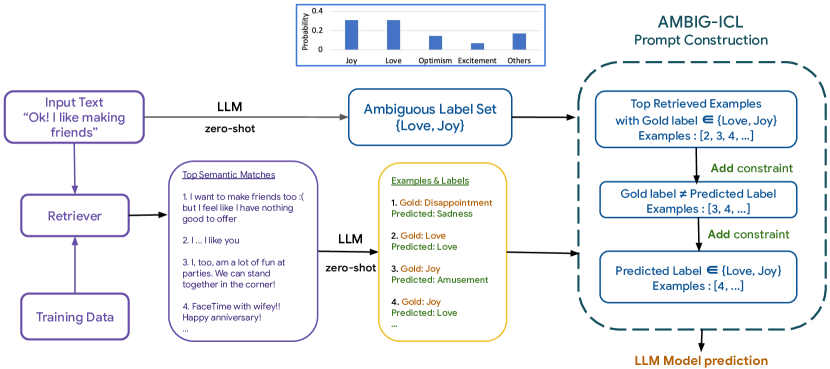
Figure 5.1: Overview of our proposed method for selecting ICL demonstrations: For each test example, we first use a retriever to rank training data by semantic similarity. At the same time, we identify the ambiguous label set for each test example and also obtain the output predictions on the retrieved training data. Next, we apply three constraints on the top-ranked demonstrations which are: 1) select those demonstrations whose gold label is in the ambiguous label set, 2) select those which are also mis-classified by the model, and 3) select those mis-classified examples whose predicted label is in the ambiguous label set. Finally, we construct prompts with selected ICL demonstrations to get the final model predictions.

As ICL gets increasingly adopted, it has brought to light [77, 29, 134, 73] that LLMs are sensitive to the choice of prompts, making “prompt engineering” for different tasks challenging and time-consuming. However, prompt engineering does not have to be a complete guessing game; rather it can be governed by some data-derived signals. For example, selecting demonstrations that are semantically similar to a new input has been shown to be more effective than randomly sampled demonstrations [33, 29, 31]. In their approaches, a text retriever is used to select the top-$k$ training examples for each test example based on the input text. The motivation is that using information from existing similar situations will help solve a new problem [136].

However, the solely input-based selection does not explicitly capture the LLM’s existing knowledge about the task-specific label space of both the ICL demonstration as well as the test input. For example, on a five-way sentiment classification task (SST [129]), we have observed that the Flan-PaLM 2 model (size L) [57] is confused between two specific labels, ‘Very Negative’ and ‘Negative,’ a lot more than say between ‘Neutral’ and ‘Very Negative’, as shown in Figure 5.2. This motivates us to investigate whether the model’s existing knowledge can also be leveraged to select even more effective demonstrations.

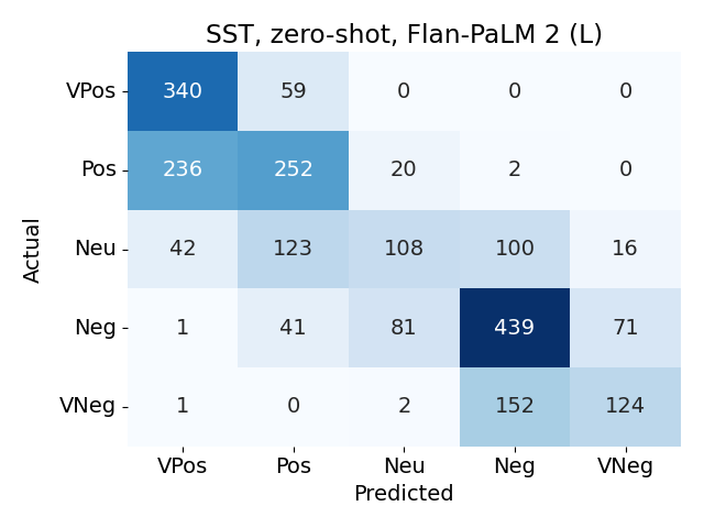
Figure 5.2: Confusion Matrix of zero-shot experiments on SST with Flan-PaLM 2 (L). Labels: VPos (Very Positive), Pos (Positive), Neu (Neutral), Neg (Negative), VNeg (Very Negative).

Specifically, we derive signals from the underlying LLM about the output label space of both the new test example and the training data from which we select the demonstrations. As motivated above, the model’s ambiguity around the new test example’s output label will help us know what the model is most confused about, which in turn can be used to select those demonstrations that help reduce this confusion. For selecting such demonstrations from the training data, we propose to consider not only the ground truth labels paired with these demonstrations, but also the usefulness by looking at their model prediction. First, given a test example and pool of training data, for each test example we use an off-the-shelf retriever to retrieve top-$k$ examples that have similar input text. For each test example, we identify an ambiguous label set of two output labels that the model is most confused about. Next, we select top-ranked demonstrations such that their ground truth labels lie in the above label set. To further find useful demonstrations, we identify those which are mis-classified by the model; the intuition is that showing the model a previously mis-classified demonstration could force it to correct it [137, 138]. Finally, on top of the mis-classified demonstrations we add a constraint to select only those demonstrations whose model prediction falls within the ambiguous label set, i.e., near the test example’s decision boundary.

To test our hypothesis, we focus on multi-class text classification tasks that have fine-grained nuance in the label space. We conduct extensive experimentation across three tasks, namely SST [129], GoEmotions [139], and EDOS (Task-B) [140], all of which have fine-grained label space, making the model more likely to be confused across labels. Our key observations are:

• Incrementally adding constraints, i.e., 1) considering label ambiguity of test example, 2) limiting ICL demonstrations to mis-classified demonstrations, and 3) considering label ambiguity of training examples leads to +1.5%, +2.2%, +2.6% improvement in F1 macro scores over the retrieval-based ICL, averaged across all datasets (Table 5.3).

• We find that adding such label-based constraints helps more on a smaller model, i.e., on Flan-PaLM 2 (M) (+3.9% gain) compared to +1.4% gain on Flan-PaLM 2 (L).

• We also attribute this success of our proposed methods to the observation that the ambiguous label set acts as a good proxy to the gold test label, and as noted by Min et al. [141], labels in the ICL demonstrations bias the model predictions the most. Therefore, showing the models the ‘likely’ gold label guides the model to make the correct prediction (Table 5.5).

5.2 Related Work

The performance of large language models (LLMs) is significantly influenced by the quality of ICL demonstrations, as demonstrated in multiple studies [120, 29, 134]. Consequently, the focus on retrieving superior demonstrations has increased. One prominent strategy is to finetune a retriever for specific tasks by similarity metrics [33, 142, 143] or by scores derived from language models [28, 144]. While some works introduce an unified retriever trained across various tasks [34, 145] for generalizabilty, another direction is to leverage off-the-shelf retrievers. Liu et al. [29] propose a KNN-based method to select ICL demonstrations based on semantic similarities; Margatina et al. [31] select ICL demonstrations with active learning algorithms based on uncertainty, diversity, and similarity, and show that selecting based on input text similarity consistently outperforms other methods; and Agrawal et al. [30] focus on selecting diverse demonstrations as well as promoting n-gram overlap between demonstrations and test examples. In our work, we adopt the off-the-shelf retriever approach as our focus is to show the generalizability of our approach across different classification tasks. However, we expect that our method will also benefit from a task-specific retriever. Additionally, to the best of our knowledge, we are the first ones to leverage the LLM’s existing knowledge surrounding the test example for selecting demonstrations. Prior works have typically explored the LLM’s existing knowledge, considering the model prediction for the training data.

Luo et al. [32] use the LLM prediction score on the training data to train a task-specific retriever, and also use Chain-of-Thought prompting [146] to improve model performance. Some works [147, 73] have found that ordering of the ICL demonstrations also affects the downstream performance, that is why in Table 5.2 we report the results across three shuffle orders. These works are orthogonal to our work but can be used in combination with our proposed methods.

5.3 Proposed Method

Typically, in an ICL regime, we assume access to training data $\mathcal{D}_{train}=\{(x_{0},y_{0}),\cdots,(x_{T},y_{T})\}$ from which the goal is to select $d$ demonstrations to be used as the prompt. As motivated in the introduction, we follow a three-step approach for selecting demonstrations: For each test example, we 1) extract semantically similar examples from $\mathcal{D}_{train}$, 2) identify the ambiguous label-set and 3) extract model predictions for $\mathcal{D}_{train}$ to identify mis-classified examples. Below, we describe each step in more detail and how they are used together to select the “best” demonstrations.

Extract Semantically Similar Demonstrations

Typically, in this approach, demonstrations are selected for each test example $x_{t}$ by finding those examples from the $\mathcal{D}_{train}$ that are semantically similar to the test input. The motivation is that observing demonstrations that are similar to the new input text will act as a hint for the model [31]. This requires the use of a retriever $R$, either an off-the-shelf one such as [29, 30, 31, 32] or a retriever trained specifically for that task [33, 28]. For each test example $x_{t}$, the retriever $R$ is used to rank examples from $\mathcal{D}_{train}$ based on semantic similarity of the text inputs. Top-$k$ input-output pairs are then selected from the ranked $\mathcal{D}_{train}$ to be used as ICL demonstrations.

Identify Ambiguous Label-Set

As we can observe from the confusion matrix in Figure 5.2, the model is often confused between two labels. We hypothesize that in addition to semantic similarity, providing demonstrations that help the model resolve this ambiguity will help the model correct itself. Thus, as a next step, we construct a prompt $\theta$ for the test example $x_{t}$, and use the model log-likelihood to score each output label $l\in L$ given the prompt. Using this we identify top-2 labels that have the highest scores, which we refer to as the “ambiguous label set” of $x_{t}$, denoted as $\mathcal{L}_{ambig,t}=\{\hat{y}_{t}^{(1)},\hat{y}_{t}^{(2)}\}$, where $\hat{y}_{t}^{(1)}$ and $\hat{y}_{t}^{(2)}$ are the first and second most likely labels, respectively.

Extract Mis-classified Demonstrations

The final component in our recipe is to consider the model prediction of the training data. While prior work [141, 148, 31] has looked at training data label-space from the lens of ground-truth labels, i.e., whether to retain them in the ICL or not, we aim to look at label-space from the perspective of model predictions. Specifically, we are interested in identifying “hard” demonstrations, i.e., examples on which the model makes mistakes. We hope that showing the model such examples with their ground truth labels will force the model to correct itself. Prior work has underscored the potential value of leveraging mis-classified examples from the training set to enhance model performance [137, 138], but it hasn’t been tested for ICL demonstration selection on text classification. In addition to the mis-classified examples, we further constrain the model prediction of these mis-classified examples to be one of the ambiguous labels, identified in the above step. Given that we already know which output labels the model is confused between for the test examples, showing the model those demonstrations (with their ground truth labels) which fall near the decision boundary will likely guide the model to choose the correct label for the test input.

5.4 Experimental Setup

5.4.1 Model

We experiment with the Flan-PaLM 2 model, an instruction-tuned model which is finetuned on the Flan dataset [149, 69] based on PaLM-2 [57], a multilingual large language model pretrained on web documents, books, code, mathematics and conversational data. We chose these models as Luo et al. [32] find that retrieved demonstration for ICL works better with instruction-tuned models than general LLMs (e.g., GPT). In particular, we experiment with two variants of the model, namely Flan-PaLM-2 (M) and Flan-PaLM-2 (L), where the latter is a larger model. The ICL demonstrations are selected using an off-the-shelf retriever which is finetuned on mT5-base [150] using the unsupervised objective proposed by Izacard et al. [151]. Since the order of demonstrations may impact the model performance [147, 73], we randomly shuffle the order of demonstrations for three random seeds and report the average results.

5.4.2 Data

As mentioned above, the Flan-PaLM 2 models are finetuned on the Flan dataset which is a mixture of many supervised datasets. Specifically, we choose three text classification datasets that satisfy the following desiderata: 1) the output label space shows fine-grained nuance that spans multiple labels, and 2) these datasets are not part of the Flan mixture to avoid any inherent bias from the underlying model. We describe them below, with dataset statistics shown in  Table 5.1. All datasets are in English.

	train	dev	test
EDOS	3,398	486	970
SST	8,544	1,101	2,210
GoEmotions	23,485	2,952	2,978

Table 5.1: Number of examples in each dataset split.

EDOS (Task-B):

The Task B of Explainable Detection of Online Sexism [140], is a topic classification task where the sexist content is classified into four categories, i.e., 1) Threats, plans to harm & incitement, 2) Derogation, 3) Animosity, and 4) Prejudiced Discussion.

SST:

The Stanford Sentiment Treebank (SST, Socher et al. [129]) is a 5-way sentiment classification dataset for movie reviews with labels: Very Negative, Negative, Neutral, Positive, and Very Positive.

GoEmotions:

The GoEmotions [139] is a multi-class sentiment classification dataset with “neutral” and 27 emotional classes, e.g., “admiration” and “fear”, collected from Reddit comments. As the label space is very large and given that we have limited sequence length, it becomes even more crucial to select a concise but effective prompt.

5.4.3 Prompt Construction

We show our templates in Table C.1 in Appendix (we use 4-shot as an example for few-shot). Task definitions are listed below, denoted by $x_{defn}$:

• EDOS: Given a text input, the task is to classify the input as being a Threat, Prejudiced, Animosity, or Derogation category of sexism. Threat refers to language where an individual expresses intent and/or encourages others to take action against women which inflicts or incites serious harm and violence against them. It includes threats of physical, sexual or privacy harm. Prejudiced refers to language which denies the existence of discrimination, and justifies sexist treatment. It includes denial and justification of gender inequality, excusing women’s mistreatment, and the ideology of male victimhood. Animosity refers to language which expresses implicit or subtle sexism, stereotypes or descriptive statements. It includes benevolent sexism, i.e., framed as a compliment. Derogation refers to language which explicitly derogates, dehumanises, demeans or insults women. It includes negative descriptions and stereotypes about women, objectification of their bodies, strong negative emotive statements, and dehumanising comparisons. It covers negative statements directed at a specific woman and women in general.

• SST: Given sentences from movie reviews, the task is to classify the sentences as being a Great, Good, Okay, Bad, or Terrible category of sentiment. Great refers to language that expresses extremely positive sentiment. Good refers to language that expresses positive sentiment, but not to the extreme. Okay refers to language that is neutral, i.e., neither expresses clear positive nor negative sentiments. Bad refers to language that expresses negative sentiment, but not to the extreme. Terrible refers to language that expresses extremely negative sentiment.

• GoEmotions: Given sentences from Reddit comments, the task is to classify the sentences as being an Admiration, Approval, Annoyance, Gratitude, Disapproval, Amusement, Curiosity, Love, Optimism, Disappointment, Joy, Realization, Anger, Sadness, Confusion, Caring, Excitement, Surprise, Disgust, Desire, Fear, Remorse, Embarrassment, Nervousness, Pride, Relief, or Grief category of emotions.

5.4.4 Baselines

We compare our proposed method against the following baselines:

Frequent Label (freq).

Select the most frequent label as the model prediction for all test examples.

Zero-shot ICL (zero).

For each test example $x_{t}$, we prepend the task definition to each test input and prompt the models. To obtain the model prediction, we use the model log-likelihood to score each output label $l\in L$, given the prompt. Then, we select the label with the highest score. $y_{t}=\operatorname*{argmax}_{L}\text{score}(l,\theta)$ where $\theta$ refers to the prompt specifically used for this setting, and score refers to the model’s log-likelihood.

Static N-shot ICL (static-$N$).

We select a fix set of $N$ demonstrations from $\mathcal{D}_{train}$, one for each of the $N$ output labels ($N=|\mathcal{L}|$). Note that these demonstrations are static for all test examples. Thus, we concatenate the task definition, $N$ demonstrations, and test example $x_{t}$ as the prompt for ICL and use the log-likelihood scores, as described above, to get the model prediction.

Retrieval-based ICL (retr).

Unlike above, where we used the same prompt for all test inputs, in this baseline, we retrieve demonstrations for each test input $x_{t}$. We use an off-the-shelf retriever $R$ (Section 5.4.1) to retrieve $k$ nearest neighbors $\{x_{1,t},\cdots,x_{k,t}\}$ from $\mathcal{D}_{train}$, similar to Das et al. [33]. We encode the input text of the training set and the test example, and rank the training data by the inner product of the vectors. Of these $k$ examples, we select $n=4,8$ as ICL demonstrations.

5.4.5 Proposed Method: Ambig-ICL

As described in Section 5.3, our proposed method considers both semantic similarity and the label ambiguity for selecting demonstrations. Below, we summarize our proposed model variants. For each setting, we first retrieve the top-$k$ most similar examples from the training data $\mathcal{D}_{train}$ for each test example $x_{t}$. We denote these candidates by $R(x_{t})=\{(x_{0,t},y_{0,t}),\cdots,(x_{k,t},y_{k,t})\}$. At the same time, for each $x_{t}$, we also identify the ambiguous label-set $\mathcal{L}_{ambig,t}=\{l_{i},l_{j}|l\in L\}$. This set contains the top-2 labels, $l_{i}$ and $l_{j}$, that the model is most confused about, where both labels belong to the set $L$ of all output labels.

+gold

Select those examples from $R(x_{t})$ as demonstrations where the ground truth label of each demonstration belongs to the ambiguous label set of $x_{t}$ denoted by:

$$\textsc{icl}(x_{t})=\left\{\begin{array}[]{ll}(x_{i},y_{i})\text{ if }y_{i}\in\mathcal{L}_{ambig,t}\\ \text{for }(x_{i},y_{i})\in R(x_{t})\end{array}\right\}$$

+gold+mis

Select those examples from $R(x_{t})$ as demonstrations where the ground truth labels fall in $\mathcal{L}_{ambig,t}$ and they are mis-classified, denoted by:

$$\textsc{icl}(x_{t})=\left\{\begin{array}[]{ll}(x_{i},y_{i})\text{ if }y_{i}\in\mathcal{L}_{ambig,t},\hat{y}_{i}\neq y_{i}\\ \text{for }(x_{i},y_{i})\in R(x_{t})\end{array}\right\}$$

Note that the model predictions ($\hat{y}$) on the $R(x_{t})$ are obtained from the zero model.

+gold+mis+pred

Select those examples from $R(x_{t})$ as demonstrations where the ground truth labels fall in $\mathcal{L}_{ambig,t}$. Ensure they are mis-classified and with an additional constraint, that their model predictions also fall within $\mathcal{L}_{ambig,t}$, denoted by:

$$\textsc{icl}(x_{t})=\left\{\begin{array}[]{ll}(x_{i},y_{i})\text{ if }y_{i}\in\mathcal{L}_{ambig,t},\hat{y}_{i}\neq y_{i},\\ \hat{y}_{i}\in\mathcal{L}_{ambig,t}\text{ for }(x_{i},y_{i})\in R(x_{t})\end{array}\right\}$$

Same as above, the model predictions on the training data are obtained from zero.

For all our proposed model variants, we select $n$ demonstrations where $n=4$ and $n=8$.

5.5 Results and Discussion

We report all our results in Table 5.2. Specifically, we use the F1 macro scores to compare the model performance, as all our tasks have unbalanced datasets. First, we note across all three tasks, our proposed methods outperform the baselines.

		EDOS		SST		GoEmotions		Avg.
		M	L	M	L	M	L	M	L
Baselines	freq	15.9	15.9	7.5	7.5	0.8	0.8	8.1	8.1
	zero	50.7	60.5	49.2	54.1	40.5	43.4	46.8	52.7
	static-$N$	51.1$\pm$0.3	58.5$\pm$0.4	50.3$\pm$0.4	56.5$\pm$0.3	34.3$\pm$0.5	44.4$\pm$0.3	45.2	53.1
	retr-4	48.5$\pm$0.3	62.3$\pm$0.4	49.9$\pm$0.3	55.4$\pm$0.3	38.3$\pm$0.3	46.2$\pm$0.4	45.6	54.6
	retr-8	47.1$\pm$0.2	61.8$\pm$0.1	51.5$\pm$0.1	55.2$\pm$0.4	37.5$\pm$0.2	46.7$\pm$0.1	45.4	54.6
Ours	Ambig-4
	+gold	49.3$\pm$0.6	62.6$\pm$0.2	51.5$\pm$0.4	56.1$\pm$0.0	40.7$\pm$0.3	48.2$\pm$0.2	47.2	55.6
	+gold+mis	52.2$\pm$0.5	61.7$\pm$0.9	52.3$\pm$0.1	57.4$\pm$0.1	40.1$\pm$0.2	47.6$\pm$0.1	48.2	55.6
	+gold+mis+pred	53.9$\pm$0.5	62.9$\pm$0.4	53.3$\pm$0.4	58.0$\pm$0.0	42.3$\pm$0.5	47.7$\pm$0.2	49.8	56.2
	Ambig-8
	+gold	47.5$\pm$0.1	63.2$\pm$0.2	52.9$\pm$0.1	56.5$\pm$0.6	42.0$\pm$1.2	47.7$\pm$0.1	47.5	55.8
	+gold+mis	50.4$\pm$0.4	62.0$\pm$0.4	53.4$\pm$0.1	57.7$\pm$0.1	43.9$\pm$0.2	47.6$\pm$0.4	49.2	55.8
	+gold+mis+pred	50.9$\pm$0.6	62.7$\pm$0.2	54.3$\pm$0.2	57.2$\pm$0.3	41.3$\pm$0.3	47.4$\pm$0.3	48.8	55.8

Table 5.2: F1 macro (%) comparison between our baselines (top) and our proposed methods (bottom) with Flan-PaLM 2 (M/L). 4 or 8 refers to the number of ICL demonstrations. The best performance across all methods is highlighted, and the best-performing baseline is underlined. The “Avg.” column shows the average scores across all datasets. The standard deviations are computed over three random seeds, with the order of demonstrations shuffled.

We also note that the zero-shot model (zero), which only uses a task definition but no task demonstrations, is already a strong baseline for both the Flan-PaLM 2 models (M/L). In particular, comparing the average scores of the few-shot baselines and zero, we find that zero outperforms few-shot baselines by 1.4% on Flan-PaLM 2 (M), but the larger model Flan-PaLM 2 (L) benefits from the addition of ICL demonstrations (+1.4% gain). This is because larger-parameter models make better use of in-context learning [152, 153, 154]. Interestingly, we also observe that for SST and GoEmotions, the Flan-PaLM 2 (L) model achieves higher performance with $n=4$ over $n=8$, which highlights that quantity does not necessarily lead to better performance.

	zero	static-$N$	Ambig-ICL    a
			+gold	+mis	+pred
M	1.3	-0.2	1.9	3.3	3.9
L	-1.9	-1.5	1.1	1.1	1.4
all	-0.3	-0.9	1.5	2.2	2.6

• We omitted retr in the table, which are inherently zero as we compare against retr.

• For both retr and Ambig-ICL, we average results on both 4 and 8 shots before computing differences.

Table 5.3: F1 macro (%) differences compared to retr, averaged across all datasets as detailed in Table 5.2. M and L refers to Flan-PaLM 2 sizes, and “all” is averaged on results of size M and L. “+mis” and “+pred” refer to “+gold+mis” and “+gold+mis+pred”, respectively.

Considering output label space is more important than semantic similarity.

Within the few-shot methods, where we use ICL demonstrations along with the task definition, we compute from Table 5.3 that our proposed methods ambig-* outperform retrieval-based models (retr-*) by +3.0% (avg.) for Flan-PaLM 2 (M), and by +1.2% (avg.) for Flan-PaLM 2 (L), suggesting that considering output label space for selecting demonstrations is as important as considering the input similarity. In particular, we find that considering mis-classified demonstrations that fall near the test example’s decision boundary leads to the overall best performance. In  Table 5.4, we show the demonstrations selected for the $n=4$ setting for one example of the GoEmotions task. We see that for the test input “Ok! I like making friends”, the retr method retrieved similar examples from $\mathcal{D}_{train}$ (all examples refer to friends). Now from the zero model, we calculated the model prediction scores and found that Love and Joy are the two labels the model is most confused about. However, because we do not consider any test example ambiguity in retr, only one of the retrieved examples represents the labels Love or Joy, which are the two labels the model is most confused about for this test example. On the other hand, in the Ambig-ICL setting, because of our constraints, all the examples chosen for ICL belong to the ambiguous label set. This allows all our proposed methods to better understand this fine-grained nuance across label space and make the correct model prediction of Love. Below, we conduct some analysis to further explain the way our proposed methods work.

Test Example: Ok! I like making friends $\mathbf{\mathcal{L}_{ambig,t}}$: Love, Joy Gold label: Love
retr	1. Disappointment: I want to make friends too :( but I feel like I have nothing good to offer 2. Joy: I, too, am a lot of fun at parties. We can stand together in the corner! 3. Gratitude: Thanks. I am. I make some new friends. 4. Disapproval: Not really. My group of friends are awesome in every way possible except they are homophobic	Predicted: Joy
Ambig-ICL
+gold	1. Joy: I, too, am a lot of fun at parties. We can stand together in the corner! 2. Love: I … I like you 3. Love: Married to the love of my life. LOL 4. Love: I do. but some people love it	Predicted: Love
+gold+mis	1. Joy: I, too, am a lot of fun at parties. We can stand together in the corner! 2. Love: Too cute for me. Why cant i have a boyfriend *[NAME]* 3. Joy: FaceTime with wifey!! Happy anniversary! 4. Love: Stick around! Would love your input POV!	Predicted: Love
+gold+mis+pred	1. Joy: FaceTime with wifey!! Happy anniversary! 2. Joy: She want to take it slow, I can see that… I deal with those girls all the time, they my favorite 3. Love: Ha! I like that one. 4. Love: Ooh I like that one :)	Predicted: Love

Table 5.4: Example demonstrations selected by the retr and our proposed method Ambig-ICL for the GoEmotions task, for $n=4$. Each demonstration comprises the input text and the ground truth label, as selected from the training data. On Flan-PaLM 2 (L), where retr mis-classified it as “Joy”, Ambig-ICL predicted correctly under all three settings.

Considering output label space compensates for the sacrifice in semantic similarity.

As we introduce more constraints (i.e., +gold, +mis, and +pred), we find that we need to sacrifice the semantic similarity to the test input. For example, consider the 4-shot Ambig-ICL experiment on EDOS (Task-B). To satisfy the constraints for the +gold setting, we need to select up to top-16 retrieved examples in order to obtain the 4 ICL demonstrations; for +gold+mis we need top-55 retrieved examples and more than top-250 retrieved examples for +gold+mis+pred. Clearly, by selecting lower ranked examples from the retrieved set $R(x_{t})$ we are sacrificing the semantic similarity to the test input. While previous studies, such as [33, 29, 31], have indicated that greater semantic similarity can enhance model performance, we can see that our methods can still outperform the retrieval-based baselines which prioritize it.

The ambiguous label set is a good proxy for the test gold label.

While Min et al. [141] find that using pseudo-demonstrations, i.e., demonstrations with random labels instead of the ground truth labels, does not affect the downstream performance much, Lyu et al. [35] find that for demonstrations that are similar to the test input, such as those from a retriever, pseudo-demonstrations hurt the performance.

	EDOS		SST		GoEmotions
	M	L	M	L	M	L
$4$-shot	42.6		29.6		21.6
$8$-shot	42.5		28.6		20.5
Ambig-4
+gold	49.5	50.3	46.5	47.1	41.3	41.9
+gold+mis	46.4	44.3	46.1	44.3	38.7	38.8
+gold+mis+pred	48.3	42.3	46.1	44.6	37.8	40.7
Ambig-8
+gold	50.3	50.3	46.0	46.8	41.2	41.7
+gold+mis	46.9	43.8	46.4	44.7	38.7	38.6
+gold+mis+pred	48.8	42.9	46.5	44.9	37.5	40.3

Table 5.5: Average percentage (%) of examples in the top $4,8$ retrieved demonstrations that share the same gold labels with the test example.

	EDOS		SST		GoEmotions
	M	L	M	L	M	L
uniform	2.00		2.32		4.75
zero	0.98	1.08	1.58	1.19	2.44	1.92
static-$N$	0.87	1.07	1.41	1.11	1.76	1.77
retr-$4$	0.78	0.97	1.40	1.06	1.89	1.70
retr-$8$	0.82	0.96	1.38	1.04	1.79	1.69
Ambig-4
+gold	0.77	0.93	1.39	1.02	1.86	1.43
+gold+mis	0.85	0.98	1.41	1.06	1.92	1.48
+gold+mis+pred	0.86	1.00	1.42	1.07	1.92	1.46
Ambig-8
+gold	0.81	0.91	1.36	0.98	1.68	1.33
+gold+mis	0.89	0.97	1.39	1.03	1.74	1.39
+gold+mis+pred	0.90	1.00	1.40	1.04	1.76	1.37

Table 5.6: Average entropy of predicted probability distribution. “uniform” refers to the entropy computed for an uniform probability distribution over the labels. Lower entropy is better.

They refer to this as the copying-effect hypothesis, which says that the “model prediction is biased towards the labels paired with the inputs in the demonstrations, especially when the inputs are similar to the test inputs.” This, in turn, suggests that the best performance could be achieved if the labels paired with the inputs are the same as the gold label of the test example. Given that we do not know the gold label of the test example apriori, the question then becomes how do we approximate the gold label?. We find that our ambiguous label set acts as a close proxy. In Table 5.5, we compute how many times the label paired with ICL demonstrations is the same as the test example gold label. We find that 44.2% of our proposed methods’ (ambig) demonstrations have the same gold label as the test example on average, compared to 30.9% from the retr method. This is why including the ambiguous label set in the demonstration selection process leads to higher performance. This analysis also sheds light on the effectiveness of retrieval-based ICL. From Table 5.5 we can see that the demonstrations selected solely based on input text similarity is only 13.3% points (avg.) behind our proposed methods. This confirms that finding demonstrations similar to the input text also leads to selecting demonstrations that have the ‘likely’ gold label.

Ambig-ICL helps reduce the model confusion.

To understand whether including test label ambiguity indeed helps decrease the model confusion, we calculate the model entropy over the predicted probability distribution of the output labels in Table 5.6. Overall, we observe that our Ambig-* methods achieve the lowest entropy across all three datasets and models. This suggests that by explicitly identifying the point of model confusion (in this case the confusion across fine-grained labels) and selecting demonstrations that help resolve this confusion is indeed effective in reducing the confusion across labels, and thereby resulting in higher downstream performance (Table 5.2). In particular, we find that for the Flan-PaLM 2 (L), the gap between the few-shot baselines and the Ambig-* methods is larger, perhaps because larger models are better able to use the ICL demonstrations [152, 153, 154].

We also compute the Pearson correlation coefficient between F1 macro scores and average entropy of the predicted probability distribution (shown in Table 5.2 and Table 5.6, respectively), for all the three datasets. We find that for the Flan-PaLM 2 (L) model, there is a negative correlation for all three datasets, i.e., $r\!=\!-0.78$ for EDOS, $-0.48$ for SST and $-0.92$ for GoEmotions, which suggests that lower entropy translates to higher task performance. However, for the Flan-PaLM 2 (M), we have mixed results, as $r$ is positive for EDOS ($0.47$), negative for SST ($-0.55$), and close to zero for GoEmotions ($0.03$).

5.6 Comparative Studies

Comparison with finetuned classifiers.

		EDOS (F1)	SST (acc.)
DistilBERT [140]		55.3	-
DeBERTa-v3-base [140]		47.9	-
BERT-large [155]		-	56.2
RoBERTa-large [155]		-	57.9
RoBERTa-large + Self-Explaining [155]		-	59.1
Heinsen Routing + RoBERTa Large [156]		-	59.8
Ambig-ICL	Flan-PaLM 2 (M)	53.9	54.2
	Flan-PaLM 2 (L)	63.2	60.2

Table 5.7: F1 macro/accuracy (%) comparison between our proposed method to finetuned classifiers on EDOS and SST.

We compare our strongest Ambig-ICL results to those of finetuned classifiers from the literature, as shown in Table 5.7.

For EDOS (Task B), both DistilBERT [157] and DeBERTa-v3-base [158] are finetuned on the training set [140]. While DistilBERT outperforms Ambig-ICL on Flan-PaLM 2 (M), it’s 7.9% behind Ambig-ICL on Flan-PaLM 2 (L) in F1 macro scores. For SST, both Sun et al. [155] and Heinsen [156] employ additional techniques beyond simple finetuning, and they perform close to but still worse than Ambig-ICL on Flan-PaLM 2 (L).

When the LLMs are larger and better at following instructions, they can be expected to outperform smaller finetuned models, especially on difficult datasets that are fine-grained and have fewer gold data. Additionally, ICL with LLMs is easily adapted to different classification tasks with only one model, whereas smaller models require finetuning for each specific task.

Additional Ambig-ICL results from literature.

We present additional results of Ambig-ICL in Table 5.8, as reported in a later study by Xu and Zhang [159]. It provides further context and presents both the strengths and limitations of the Ambig-ICL approach.

	Macro-F1
	GLUE	Ethos	TweetEval	HateS18	Poem	Average
Uniform	$75.5$	$65.5$	$63.7$	$63.7$	$68.7$	$67.4$
Best-of-10 [134]	$75.8$	$69.1$	68.8	$70.6$	$72.2$	71.3
Topic [160]	$76.2$	$62.4$	-	-	75.2	-
KATE [29]	$72.3$	$71.2$	$66.3$	$66.8$	$73.2$	$69.9$
Ambig-ICL	76.6	71.3	$68.3$	72.4	$67.7$	71.3
ICR [159]	$\mathbf{78.7}$	$\mathbf{76.5}$	$\mathbf{71.0}$	$\mathbf{74.4}$	$\mathbf{76.5}$	$\mathbf{75.4}$

Table 5.8: F1 macro (%) reported by Xu and Zhang.

Xu and Zhang [159] proposed In-Context Reflection (ICR), a method designed to identify demonstrations that are most likely to challenge the understanding of LLMs. They tested their approach on several benchmark datasets, including GLUE [161], Ethos [162], TweetEval [163], HateS18 [164], and Poem [165]. Their comparison results are shown in Table 5.8, and Ambig-ICL outperforms all other methods, except ICR, on 3 out of the 5 datasets.

For TweetEval, they adopted three subtasks: “Hate Speech Detection”, “Emotion Recognition”, and “Irony Detection”, and reported the average score. Given that “Hate” and “Irony” are binary classification tasks, while “Emotion” is a 4-way classification task, TweetEval may be considered a less fine-grained dataset, which could make Ambig-ICL less preferable in this context. Poem is a 4-way sentiment classification task for poems of different verses. As we lack access to label-wise results, it’s difficult to determine the reason for failure. However, Topic [160], which learns latent concepts, achieves the best performance, offering potential insights into achieving higher performance on the Poem dataset. We note that the authors didn’t define the labels (negative/positive/neutral/mixed) in their prompt as we did in our experiments. This may have added to the model’s difficulty in understanding the classes, leading to a flawed ambiguous label set selection.

While our method has demonstrated promising results across various datasets, potential pitfalls remain. If the actual gold label of test example often deviates from the LLM’s top two label choices in a particular dataset or model, this can indicate subpar zero-shot performance or flawed ambiguous label set selection. In these scenarios, our method may lead to unsatisfying performance, necessitating further enhancements. To mitigate these issues and improve overall performance, we encourage specifying task instructions and label definitions in the prompt.

5.7 Conclusion

In this work, we find that using LLM’s existing knowledge (e.g., the model prediction) regarding the output label space of both the test example and the ICL demonstration pool is as important as considering the semantic similarity of the input text alone. We find that our proposed methods consistently outperform the baselines for all three tasks. Although we only consider the top-2 most ambiguous labels in selecting the ICL demonstrations, it would be interesting to expand the ambiguous label set to more than two labels. This would especially be more important for datasets like GoEmotions where the label space is large and much more fine-grained. We leave this effort for future work. Furthermore, in this work, we focus on sentence classification tasks, thus paving the way for others to use our proven techniques to also explore label ambiguity for other token/span-level tasks such as Named Entity Recognition (NER), and Part-Of-Speech (POS) tagging.

Chapter 6 Conclusion

6.1 Summary of Contributions

This thesis has explored the advancements in text classification by harnessing Pretrained Language Models (PLMs) to address three challenging settings: distractor selection for multiple-choice cloze questions, prompt-based zero-shot text classification, and demonstration selection for retrieval-based in-context learning. The main contributions are:

Distractor Analysis and Selection for Multiple-Choice Cloze Questions.

• Experimented on two datasets specifically tailored for evaluating distractor selection in multiple-choice cloze questions. One dataset consists of standalone cloze sentences, while the other includes the cloze sentence within a paragraph. Given the usual lack of direct supervision in past works, the analysis and results provide valuable insights for this domain.

• Designed context-free features as well as context-sensitive features with contextualized word representations derived from PLMs. We find models tend to favor syntactically correct distractors while differing sufficiently in semantics.

• Demonstrated that the use of PLMs significantly enhances the performance of distractor selection models, achieving results comparable to or exceeding human annotators. Detailed quantitative analysis provided insights into the relative importance of different model components and features.

Label-Description Training for Zero-Shot Text Classification.

• Proposed to craft small datasets that describe task labels for zero-shot text classification, applicable for both finetuning and in-context learning.

• Showed that this label-description training method improves accuracy by 17-19% over traditional zero-shot approaches across multiple topic and sentiment classification datasets. The method also demonstrated robustness to variations in patterns and verbalizers, and LabelDesc data can partially compensate when the quality of the verbalizers is unknown or poor.

• Highlighted the domain-independent nature of the approach. In several cases, this method outperformed few-shot learning on out-of-domain datasets.

Ambiguity-Aware In-Context Learning with Large Language Models.

• Developed a method for in-context learning that selects demonstrations based on model predictions of both demonstrations and test examples, thereby resolving the model ambiguity about test example labels.

• Conducted extensive experiments on fine-grained text classification tasks, demonstrating that the proposed method improves F1 macro scores by up to 2.6% over traditional retrieval-based in-context learning approaches.

• Found that the set of the top two most likely labels is a good proxy for the gold label of a test example, shedding light on the effectiveness of retrieval-based ICL.

6.2 Future Work

While distractor selection is a highly practical application, designing distractors to better assist student learning remains an area for further exploration, and this domain still lacks sufficient datasets. Future work can use our models to collect more training data and delve deeper into the different decisions students make. Additionally, exploring the usage of question answering PLMs could be beneficial. For example, can question answering PLMs simulate students’ answers, and how accurately can they capture them? Are the current annotation rules the best practice? Aside from language learning, could we expand to other disciplines?

In Chapter 4 and Chapter 5, both LabelDescTraining and Ambig-ICL were tested on topic and sentiment classification tasks. A future direction is to apply these methods to other span-level tasks, such as Named Entity Recognition (NER) and Part-Of-Speech (POS) tagging, as well as to natural language generation tasks, such as generating text in different styles. Another research avenue would be to explore ways to improve the consistency of models regarding patterns and verbalizers, such as debiasing through calibration. Additionally, the mechanisms underlying retrieval-based ICL are still not fully understood, and the interaction of multiple demonstrations within a single prompt requires further study.

Although all tasks in this thesis are conducted in English, it would be interesting to harness PLMs’ intrinsic knowledge for cross-linguistic knowledge transfer. Different languages encode and represent knowledge in different ways. For instance, in French, the number eighty is expressed as “quatre-vingts,” where “quatre” means “four” and “vingts” means “twenties.” This linguistic construction involves a mathematical operation, even though it is not explicitly stated. Investigating how well PLMs can transfer this type of numerical and linguistic knowledge from one language to another could open new possibilities for multilingual applications, including text classification.

Appendix A Appendix to Chapter 3

A.1 Dataset

There are some problematic words in the dataset, such as ‘testing, test’, ‘find s’, ‘find ed’ in MCDSent/MCDPara candidate words. There are also some extra spaces (or non-breaking spaces) at the start or end of words. To keep the words the same as what the annotators saw, we only remove leading/trailing white space, and replace non-breaking spaces with ordinary spaces. By comparing the percentages of the circumstances where spaces are included in the string before/after tokenization, we find the percentage of extra spaces presented in Table A.1. The vocabulary size after tokenization is presented in Table A.2.

%	headword$(c)$	$c$	headword$(d)$	$d$
MCDSent	0	0	0.0168	0.0332
MCDPara	0.0160	0.0307	0.0364	0.0622

Table A.1: Percentage of extra spaces (excluding those that are in the middle of words), where headword$(c)$ denotes headword of correct answer, and $d$ denotes distractor candidates of inflected forms .

	headword$(c)$	$c$	headword$(d)$	$d$
MCDSent	2571	2731	3514	11423
MCDPara	2683	4174	3582	13749

Table A.2: Vocabulary sizes.

A.1.1 Distractor Annotation

The software tool suggested distractor candidates based on the following priority ranking:

• It is in a proprietary dictionary.

• It has the same part-of-speech (POS) as the correct answer (if POS data is available) and satisfies 1.

• It is part of a proprietary learnable word list for the language learning course under consideration, and satisfies 2.

• It is in the same course as the correct answer and satisfies 3.

• It is in the same proprietary study material bundle as the correct answer and satisfies 4.

• It is in the previous or same study material as the correct answer and satisfies 5.

• It is in the same study material as the correct answer and satisfies 6.

• It is in the same NGSL frequency word list band as the correct answer and satisfies 7.

• It is not used as a distractor for another word with the same task type in the same material at the time that the distractor list for quality assurance (QA) is loaded, and satisfies 8.

%	sent start	sent end	para start	para end
MCDSent	3.058	0.005	-	-
MCDPara	2.640	0.342	18.272	22.165

Table A.3: Position of the candidates, where “sent” denotes sentence and “para” denotes paragraph. “para start” means that the sentence containing the blank is at the beginning of the paragraph.

A.1.2 Context Position

Sometimes the blank resides at the start or end of the context (a sentence for MCDSent, and a paragraph for MCDPara), counts of which are shown in Table A.3. The percentage when there is only one sentence as context in MCDPara is 0.894%.

A.2 Results Tuned Based on F1

We report our results tuned based on F1 in Table A.4 and A.5.

model	variant	development set				test set				BERT	features	best	threshold
		precision	recall	F1	AUPR	precision	recall	F1	AUPR			epoch
baseline		15.4	100	26.7	-	13.3	100	23.5	-	-	-	-	-
		33.3	64.8	44.0	35.1	23.2	59.1	33.3	25.0	none	yes	26	0.2
$M_{\textit{feat}}$		42.1	67.0	51.7	45.4	31.5	57.4	40.7	32.3	base	yes	26	0.2
		41.3	67.1	51.1	46.7	32.4	56.6	41.2	33.9	large	yes	25	0.3
	none	49.0	79.1	60.5	58.5	46.5	75.7	57.6	53.9	-	no	6	0.3
	gru+c	49.7	77.6	60.6	54.1	46.1	73.3	56.7	53.5	-	no	3	0.4
$M_{\textit{ELMo}}$	all	52.9	75.8	62.3	60.4	48.0	75.9	58.8	57.6	-	no	2	0.4
	none	51.0	84.0	63.4	63.1	47.7	81.4	60.1	60.6	large	yes	3	0.3
	gru+c	56.9	72.3	63.7	59.1	50.6	75.9	60.8	58.6	large	yes	5	0.4
	all	53.5	80.8	64.4	63.4	50.8	75.5	60.8	59.6	large	yes	3	0.4
		48.8	85.5	62.1	56.6	43.8	82.8	57.3	51.5	base	no	4	0.2
$M_{\textit{BERT}}$		49.6	80.8	61.5	59.1	45.2	79.7	57.7	54.9	large	no	3	0.3
		51.5	84.2	63.9	61.7	46.0	78.6	58.0	55.0	base	yes	6	0.2
		51.4	81.1	62.9	64.7	46.4	79.8	58.7	57.5	large	yes	6	0.2

Table A.4: Results for MCDSent tuned based on F1.

model	development set				test set				BERT	features	best epoch	threshold
	precision	recall	F1	AUPR	precision	recall	F1	AUPR
baseline	7.3	100	13.5	-	6.6	100	12.4	-	-	-	-	-
	17.1	53.1	25.9	15.9	15.6	51.3	23.9	15.0	-	yes	14	0.1
$M_{\textit{feat}}$	19.5	63.0	29.8	20.4	17.6	61.0	22.3	18.6	base	yes	22	0.1
	20.4	63.1	30.8	22.3	16.7	62.7	26.4	18.6	large	yes	25	0.1
$M_{\textit{ELMo}}$	35.2	55.4	43.1	37.0	31.2	54.6	39.8	33.9	-	no	5	0.3
	40.2	61.3	48.5	43.8	34.1	59.4	43.3	35.2	large	yes	5	0.3
$M_{\textit{ELMo}}(\ell)$	28.7	72.9	41.2	33.8	25.7	71.3	37.7	30.3	-	no	2	0.2
	36.2	67.3	47.1	40.8	31.0	65.6	42.1	37.3	large	yes	7	0.3
	35.8	64.2	46.0	39.3	28.9	64.3	39.9	34.5	base	no	5	0.2
$M_{\textit{BERT}}$	35.2	62.1	45.0	38.3	26.9	60.5	37.3	29.3	large	no	6	0.1
	44.3	55.4	49.3	47.3	34.6	56.2	42.8	36.7	base	yes	2	0.3
	37.8	63.3	47.4	44.0	32.7	66.1	43.7	38.1	large	yes	3	0.2
$M_{\textit{BERT}}(\ell)$	34.0	64.3	44.5	36.7	29.6	62.1	40.1	32.1	base	no	5	0.2
	43.3	57.5	49.4	45.4	33.3	60.9	43.1	35.8	base	yes	3	0.3

Table A.5: Results for MCDPara tuned based on F1.

A.3 Supplement for Analysis

The example for MCDPara is as below, and two sets of its distractors are shown in Figure A.1.

• MCDPara: A few years have passed since the Great Tohoku Earthquake occurred. It has been extremely costly to rebuild the damaged areas from scratch, with well over $200 billion dollars provided for reconstruction. However, the availability of these funds has been limited. However, a large portion of the money has been kept away from the victims due to a system which favors construction companies….

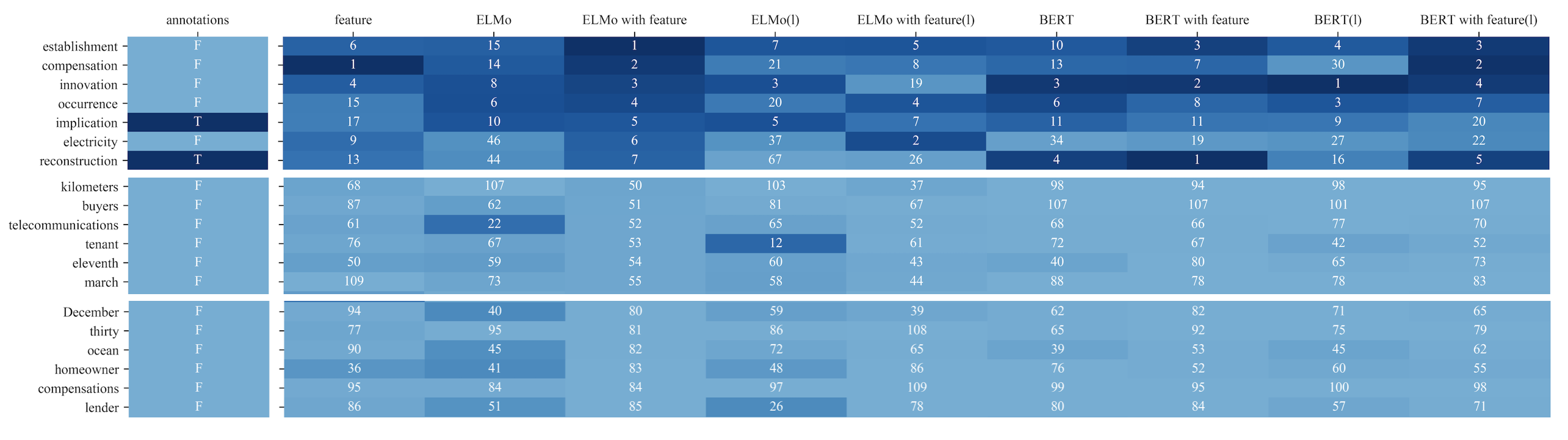
Figure A.1: Ranks for distractor candidates of MCDPara question “However, the availability of these funds has been limited.” along with annotations.

Appendix B Appendix to Chapter 4

B.1 Domain Transfer

All results on RoBERTa-base/large are shown in Figure B.1 and B.2.

B.1

Figure B.1: Domain transfer results of topic classification, where X-axis depicts the number of training examples per label. “base/large” in parenthesis denotes RoBERTa-base/large.

B.1

Figure B.2: Domain transfer results of sentiment classification, where X-axis depicts the number of training examples per label. “base/large” in parenthesis denotes RoBERTa-base/large.

B.2 LabelDesc Data

The statistics of LabelDesc data are shown in Table 4.2. We use the same set of LabelDesc data for AGNews and Yahoo${}_{\textrm{AG}}$, Yelp-5 and SST-5, Yelp-2 and SST-2, respectively. The data is listed in Table B.1 - Table B.4. Each term/sentence that is separated by “|” in tables is an independent LabelDesc example during training. For brevity, we list all hand-crafted templates instead of listing all data for sentiment classification.

Label	Type	Training Data
talk. religion. misc	terms	religion | Christian | Buddhist | Jewish
	Wiki.	Religion is usually defined as a social-cultural system of designated behaviors and practices, morals, beliefs, worldviews, texts, sanctified places, prophecies, ethics, or organizations, that generally relates humanity to supernatural, transcendental, and spiritual elements; however, there is no scholarly consensus over what precisely constitutes a religion.
	dict.	a set of beliefs concerning the cause, nature, and purpose of the universe, especially when considered as the creation of a superhuman agency or agencies, usually involving devotional and ritual observances, and often containing a moral code governing the conduct of human affairs.
rec.autos	terms	automobile | truck | car | vehicle
	Wiki.	A car (or automobile) is a wheeled motor vehicle that is used for transportation.
	dict.	a passenger vehicle designed for operation on ordinary roads and typically having four wheels and a gasoline or diesel internal-combustion engine.
sci.med	terms	medicine | hospital | symptom | cure
	Wiki.	Medicine is the science and practice of caring for a patient, managing the diagnosis, prognosis, prevention, treatment, palliation of their injury or disease, and promoting their health.
	dict.	any substance or substances used in treating disease or illness; medicament; remedy.
talk. politics. guns	terms	gun | firearm | weapon | handgun
	Wiki.	A gun is a ranged weapon designed to use a shooting tube (gun barrel) to launch projectiles.
	dict.	a weapon consisting of a metal tube, with mechanical attachments, from which projectiles are shot by the force of an explosive; a piece of ordnance.

Table B.1: LabelDesc data for 20NG. “Wiki.” and “dict.” refers to the data source, i.e., Wikipedia or dictionary definition.

Label	Type	Training Data
Negative	terms	awful | terrible | horrendous | horrible | dreadful | bad | unpleasant | unsatisfying | lousy | subpar
	sent.	It was $t$. | A(n) $t$ experience. | Just $t$. | Overall, it was $t$.
Positive	terms	good | nice | fine | pleasant | neat | great | amazing | excellent | fantastic | outstanding
	sent.	It was $t$. | A(n) $t$ experience. | Just $t$. | Overall, it was $t$.

Table B.2: LabelDesc data for Yelp-2, SST-2, Amz-2 and IMDB.

Label	Type	Training Data
Society & Culture	terms	society | culture
	Wiki.	A society is a group of individuals involved in persistent social interaction, or a large social group sharing the same spatial or social territory, typically subject to the same political authority and dominant cultural expectations. | Culture is an umbrella term which encompasses the social behavior, institutions, and norms found in human societies, as well as the knowledge, beliefs, arts, laws, customs, capabilities, and habits of the individuals in these groups.
	dict.	an organized group of persons associated together for religious, benevolent, cultural, scientific, political, patriotic, or other purposes. | the behaviors and beliefs characteristic of a particular group of people, as a social, ethnic, professional, or age group (usually used in combination)
Science & Mathematics	terms	science | mathematics
	Wiki.	Science is a systematic endeavor that builds and organizes knowledge in the form of testable explanations and predictions about the universe. | Mathematics is an area of knowledge that includes such topics as numbers, formulas and related structures, shapes and the spaces in which they are contained, and quantities and their changes.
	dict.	a branch of knowledge or study dealing with a body of facts or truths systematically arranged and showing the operation of general laws | the systematic treatment of magnitude, relationships between figures and forms, and relations between quantities expressed symbolically.
Health	terms	health | fitness | medical | diet
	Wiki.	Health, according to the World Health Organization, is “a state of complete physical, mental and social well-being and not merely the absence of disease and infirmity”.
	dict.	the general condition of the body or mind with reference to soundness and vigor
Education & Reference	terms	education | reference
	Wiki.	Education is a purposeful activity directed at achieving certain aims, such as transmitting knowledge or fostering skills and character traits. | Reference is a relationship between objects in which one object designates, or acts as a means by which to connect to or link to, another object.
	dict.	the act or process of imparting or acquiring general knowledge, developing the powers of reasoning and judgment, and generally of preparing oneself or others intellectually for mature life. | a book or other source of useful facts or information, such as an encyclopedia, dictionary, etc.
Computers & Internet	terms	computer | internet
	Wiki.	A computer is a digital electronic machine that can be programmed to carry out sequences of arithmetic or logical operations (computation) automatically. | The Internet (or internet) is the global system of interconnected computer networks that uses the Internet protocol suite (TCP/IP) to communicate between networks and devices.
	dict.	a programmable electronic device designed to accept data, perform prescribed mathematical and logical operations at high speed, and display the results of these operations. Mainframes, desktop and laptop computers, tablets, and smartphones are some of the different types of computers. | Usually the internet (except when used before a noun). a vast computer network linking smaller computer networks worldwide. The internet includes commercial, educational, governmental, and other networks, all of which use the same set of communications protocols
Sports	terms	sport | sports | racing | baseball
	Wiki.	Sport pertains to any form of competitive physical activity or game that aims to use, maintain or improve physical ability and skills while providing enjoyment to participants and, in some cases, entertainment to spectators.
	dict.	an athletic activity requiring skill or physical prowess and often of a competitive nature, as racing, baseball, tennis, golf, bowling, wrestling, boxing, hunting, fishing, etc.
Business & Finance	terms	business | finance
	Wiki.	Business is the activity of making one’s living or making money by producing or buying and selling products (such as goods and services). | Finance is the study and discipline of money, currency and capital assets.
	dict.	the purchase and sale of goods in an attempt to make a profit. | the management of revenues; the conduct or transaction of money matters generally, especially those affecting the public, as in the fields of banking and investment.
Entertainment & Music	terms	entertainment | music
	Wiki.	Entertainment is a form of activity that holds the attention and interest of an audience or gives pleasure and delight. | Music is generally defined as the art of arranging sound to create some combination of form, harmony, melody, rhythm or otherwise expressive content.
	dict.	the act of entertaining; agreeable occupation for the mind; diversion; amusement | an art of sound in time that expresses ideas and emotions in significant forms through the elements of rhythm, melody, harmony, and color.
Family & Relationships	terms	family | relationship
	Wiki.	Family is a group of people related either by consanguinity (by recognized birth) or affinity (by marriage or other relationship). | The concept of interpersonal relationship involves social associations, connections, or affiliations between two or more people.
	dict.	a basic social unit consisting of parents and their children, considered as a group, whether dwelling together or not; a social unit consisting of one or more adults together with the children they care for. | an emotional or other connection between people
Politics & Government	terms	politics | government
	Wiki.	Politics is the set of activities that are associated with making decisions in groups, or other forms of power relations among individuals, such as the distribution of resources or status. | A government is the system or group of people governing an organized community, generally a state.
	dict.	the science or art of political government. | the political direction and control exercised over the actions of the members, citizens, or inhabitants of communities, societies, and states; direction of the affairs of a state, community, etc.; political administration

Table B.3: LabelDesc data for Yahoo Answers.

Label	Type	Training Data
Company	terms	company | firm | corporation | business
	Wiki.	A company, abbreviated as co., is a legal entity representing an association of people, whether natural, legal or a mixture of both, with a specific objective.
	dict.	a number of persons united or incorporated for joint action, especially for business
Educational Institution	terms	educational institution | university | college | school
	Wiki.	An educational institution is a place where people of different ages gain an education, including preschools, childcare, primary-elementary schools, secondary-high schools, and universities.
	dict.	an institution for instruction in a particular skill or field.
Artist	terms	artist | writer | actor | singer
	Wiki.	An artist is a person engaged in an activity related to creating art, practicing the arts, or demonstrating an art.
	dict.	a person who produces works in any of the arts that are primarily subject to aesthetic criteria.
Athlete	terms	athlete | sports | footballer | weightlifter
	Wiki.	An athlete (also sportsman or sportswoman) is a person who competes in one or more sports that involve physical strength, speed, or endurance.
	dict.	a person trained or gifted in exercises or contests involving physical agility, stamina, or strength; a participant in a sport, exercise, or game requiring physical skill.
Office Holder	terms	office-holder | politics | mayor | president
	Wiki.	A person who’s been appointed to a position by a company or organisation but doesn’t have a contract or receive regular payment may be an office-holder.
	dict.	a person filling a governmental position; public official.
Mean of Transportation	terms	mean of transportation | car | bus | train
	Wiki.	Transport (in British English), or transportation (in American English), is the intentional movement of humans, animals, and goods from one location to another.
	dict.	a means of transporting or conveying, as a truck or bus.
Building	terms	building | apartment | skyscraper | tower
	Wiki.	A building or edifice, is an enclosed structure with a roof and walls standing more or less permanently in one place, such as a house or factory (although there’s also portable buildings).
	dict.	a relatively permanent enclosed construction over a plot of land, having a roof and usually windows and often more than one level, used for any of a wide variety of activities, as living, entertaining, or manufacturing.
Natural Place	terms	natural place | forest | mountain | river
	Wiki.	The natural environment or natural world encompasses all living and non-living things occurring naturally, meaning in this case not artificial.
	dict.	existing in or formed by nature (opposed to artificial)
Village	terms	village | town | countryside | rural
	Wiki.	A village is a clustered human settlement or community, larger than a hamlet but smaller than a town (although the word is often used to describe both hamlets and smaller towns), with a population typically ranging from a few hundred to a few thousand.
	dict.	a small community or group of houses in a rural area, larger than a hamlet and usually smaller than a town, and sometimes (as in parts of the U.S.) incorporated as a municipality.
Animal	terms	animal | insect | bird | fish
	Wiki.	Animals are multicellular, eukaryotic organisms in the biological kingdom Animalia.
	dict.	any member of the kingdom Animalia, comprising multicellular organisms that have a well-defined shape and usually limited growth, can move voluntarily, actively acquire food and digest it internally, and have sensory and nervous systems that allow them to respond rapidly to stimuli: some classification schemes also include protozoa and certain other single-celled eukaryotes that have motility and animallike nutritional modes.
Plant	terms	plant | flower | tree | grass
	Wiki.	Plants are predominantly photosynthetic eukaryotes, forming the kingdom Plantae.
	dict.	Botany. any member of the kingdom Plantae, comprising multicellular organisms that typically produce their own food from inorganic matter by the process of photosynthesis and that have more or less rigid cell walls containing cellulose, including vascular plants, mosses, liverworts, and hornworts: some classification schemes may include fungi, algae, bacteria, and certain single-celled eukaryotes that have plantlike qualities, as rigid cell walls or the use of photosynthesis.
Album	terms	album | soundtrack | mixtape | CD
	Wiki.	An album is a collection of audio recordings issued on compact disc (CD), vinyl, audio tape, or another medium such as digital distribution.
	dict.	a record or set of records containing several musical selections, a complete play or opera, etc.
Film	terms	film | movie | comedy | drama
	Wiki.	A film – also called a movie, motion picture, moving picture, picture, photoplay or (slang) flick – is a work of visual art that simulates experiences and otherwise communicates ideas, stories, perceptions, feelings, beauty, or atmosphere through the use of moving images.
	dict.	a sequence of consecutive still images recorded in a series to be viewed on a screen in such rapid succession as to give the illusion of natural movement; motion picture.
Written Work	terms	written work | novel | newspaper | book
	Wiki.	A book is a medium for recording information in the form of writing or images, typically composed of many pages (made of papyrus, parchment, vellum, or paper) bound together and protected by a cover.
	dict.	a handwritten or printed work of fiction or nonfiction, usually on sheets of paper fastened or bound together within covers.

Table B.4: LabelDesc data for DBPedia.

Appendix C Appendix to Chapter 5

C.1 Prompt Construction Template

$x_{defn}$ Thus given the following input:
input: $x_{t}$
answer: $x_{defn}$ Some examples are:
input: $x_{1,t}$
answer: $y_{1,t}$

input: $x_{2,t}$
answer: $y_{2,t}$

input: $x_{3,t}$
answer: $y_{3,t}$

input: $x_{4,t}$
answer: $y_{4,t}$

Thus given the following input:
input: $x_{t}$
answer:

Table C.1: Prompt templates for zero-shot and few-shot ICL. $x_{t}$ refers to the test example, and $x_{i,t},y_{i,t}$ refers to the text inputs and gold labels of ICL demonstrations selected for $x_{t}$, respectively.

C.2 Accuracy, Precision, Recall

Please refer to Table C.2, C.3 and C.4.

		EDOS		SST		GoEmotions
		M	L	M	L	M	L
Baselines	freq	11.7	11.7	4.6	4.6	0.4	0.4
	zero	65	60.7	54	56.2	42.6	46.3
	static-$N$	65.2$\pm$0.6	58.1$\pm$0.4	54.5$\pm$0.6	58.2$\pm$0.3	42.6$\pm$1.2	46.2$\pm$0.3
	retr-4	67.1$\pm$1.1	63.6$\pm$0.5	53.4$\pm$0.3	57.4$\pm$0.4	43.7$\pm$0.4	47.6$\pm$0.4
	retr-8	65.0$\pm$0.2	63.9$\pm$0.3	54.4$\pm$0.1	57.6$\pm$0.5	43.7$\pm$0.4	48.3$\pm$0.1
Ours	Ambig-4
	+gold	65.9$\pm$0.8	63.6$\pm$0.4	54.1$\pm$0.3	57.7$\pm$0.1	45.7$\pm$0.3	50.5$\pm$0.2
	+gold+mis	66.6$\pm$1.1	63.6$\pm$1.0	54.1$\pm$0.2	58.8$\pm$0.1	44.8$\pm$0.4	49.2$\pm$0.1
	+gold+mis+pred	67.4$\pm$0.4	65.0$\pm$0.5	54.8$\pm$0.5	59.4$\pm$0.0	46.9$\pm$1.3	47.9$\pm$0.2
	Ambig-8
	+gold	66.4$\pm$1.1	64.8$\pm$0.1	54.7$\pm$0.2	58.5$\pm$0.7	48.0$\pm$1.8	49.9$\pm$0.1
	+gold+mis	68.4$\pm$0.8	64.4$\pm$0.6	54.5$\pm$0.1	59.6$\pm$0.1	48.7$\pm$0.5	48.8$\pm$0.5
	+gold+mis+pred	66.6$\pm$1.2	66.4$\pm$0.3	54.9$\pm$0.2	59.1$\pm$0.4	43.7$\pm$0.5	47.4$\pm$0.3

Table C.2: Precision (%) comparison between our proposed methods and baselines with Flan-PaLM 2 (M, L).

		EDOS		SST		GoEmotions
		M	L	M	L	M	L
Baselines	freq	25	25	20	20	3.7	3.7
	zero	46	62.8	53.8	55.2	42.4	47.2
	static-$N$	46.2$\pm$0.3	63.0$\pm$0.3	54.0$\pm$0.4	56.5$\pm$0.2	34.8$\pm$0.5	49.5$\pm$0.4
	retr-4	44.8$\pm$0.3	63.4$\pm$0.2	53.4$\pm$0.3	55.7$\pm$0.3	38.5$\pm$0.2	49.7$\pm$0.3
	retr-8	44.0$\pm$0.1	62.1$\pm$0.2	54.2$\pm$0.1	55.3$\pm$0.4	37.8$\pm$0.3	50.1$\pm$0.3
Ours	Ambig-4
	+gold	45.1$\pm$0.6	64.1$\pm$0.2	54.6$\pm$0.4	56.4$\pm$0.1	41.4$\pm$0.3	51.3$\pm$0.2
	+gold+mis	48.0$\pm$0.4	62.1$\pm$0.9	54.9$\pm$0.1	57.3$\pm$0.1	40.9$\pm$0.1	51.0$\pm$0.4
	+gold+mis+pred	49.5$\pm$0.4	63.1$\pm$0.3	55.6$\pm$0.4	57.7$\pm$0.0	42.7$\pm$0.2	51.7$\pm$0.4
	Ambig-8
	+gold	43.6$\pm$0.1	64.0$\pm$0.2	55.0$\pm$0.1	56.5$\pm$0.6	41.9$\pm$0.9	50.8$\pm$0.5
	+gold+mis	47.3$\pm$0.4	61.8$\pm$0.3	54.9$\pm$0.1	57.3$\pm$0.1	44.4$\pm$0.2	51.4$\pm$0.3
	+gold+mis+pred	48.0$\pm$0.4	61.7$\pm$0.2	55.6$\pm$0.2	56.7$\pm$0.2	43.2$\pm$0.3	51.3$\pm$0.1

Table C.3: Recall (%) comparison between our proposed methods and baselines with Flan-PaLM 2 (M, L).

		EDOS		SST		GoEmotions
		M	L	M	L	M	L
Baselines	freq	46.8	46.8	23.1	23.1	11.7	11.7
	zero	55.4	59.2	49.9	57.1	47.1	46.2
	static-$N$	54.3$\pm$0.3	57.6$\pm$0.1	50.5$\pm$0.4	59.0$\pm$0.2	39.8$\pm$0.2	46.7$\pm$0.2
	retr-4	53.6$\pm$0.3	61.0$\pm$0.5	50.0$\pm$0.3	58.5$\pm$0.3	45.9$\pm$0.0	50.1$\pm$0.2
	retr-8	53.8$\pm$0.3	61.1$\pm$0.2	51.8$\pm$0.1	58.6$\pm$0.4	45.3$\pm$0.0	51.0$\pm$0.2
Ours	Ambig-4
	+gold	54.3$\pm$0.4	61.3$\pm$0.4	51.5$\pm$0.4	58.9$\pm$0.1	46.6$\pm$0.2	50.3$\pm$0.1
	+gold+mis	56.1$\pm$0.2	60.9$\pm$0.6	52.1$\pm$0.1	59.7$\pm$0.1	45.6$\pm$0.1	49.5$\pm$0.1
	+gold+mis+pred	56.5$\pm$0.1	61.4$\pm$0.4	53.0$\pm$0.4	60.1$\pm$0.1	45.6$\pm$0.1	50.0$\pm$0.2
	Ambig-8
	+gold	53.6$\pm$0.2	61.8$\pm$0.0	52.9$\pm$0.1	59.5$\pm$0.6	46.8$\pm$0.1	50.4$\pm$0.2
	+gold+mis	55.4$\pm$0.6	61.1$\pm$0.3	53.2$\pm$0.1	60.2$\pm$0.1	45.8$\pm$0.2	50.0$\pm$0.3
	+gold+mis+pred	55.1$\pm$0.6	61.5$\pm$0.3	54.2$\pm$0.2	59.6$\pm$0.3	44.9$\pm$0.2	50.2$\pm$0.2

Table C.4: Accuracy (%) comparison between our proposed methods and baselines with Flan-PaLM 2 (M, L).

C.3 Label-wise Percentage Analysis of Gold Label Inclusion in $\mathbf{\mathcal{L}_{ambig,t}}$

We compute the percentage of times that the test example’s gold label is in $\mathcal{L}_{ambig,t}$ (as obtained with zero) in Table C.5, and we present label-wise results in Table C.6.

	EDOS	SST	GoEmotions
Flan-PaLM 2 (M)	91.2	85.8	61.2
Flan-PaLM 2 (L)	88.2	87.6	61.6

Table C.5: Percentage of times the test example’s gold label is in $\mathcal{L}_{ambig,t}$ (as obtained from zero model).

EDOS	M	Animosity 99.1, Derogation 97.4, Prejudiced 52.1, Threat 71.9
	L	Animosity 90.1, Derogation 90.1, Prejudiced 68.1, Threat 93.3
SST	M	Bad 78.4, Good 98.0, Great 88.0, Okay 73.8, Terrible 93.9
	L	Bad 89.3, Good 99.2, Great 99.2, Okay 59.1, Terrible 85.3
GoEmotions	M	Admiration 72.7, Amusement 90.3, Anger 58.8, Annoyance 44.3, Approval 24.6, Caring 52.9, Confusion 73.2, Curiosity 64.2, Desire 35.7, Disappointment 58.0, Disapproval 52.3, Disgust 55.3, Embarrassment 30.4, Excitement 56.4, Fear 75.4, Gratitude 75.7, Grief 100.0, Joy 80.4, Love 86.8, Nervousness 83.3, Optimism 51.4, Pride 42.9, Realization 27.0, Relief 28.6, Remorse 38.6, Sadness 71.6, Surprise 62.1
	L	Admiration 40.2, Amusement 84.9, Anger 52.7, Annoyance 40.2, Approval 36.0, Caring 36.5, Confusion 74.2, Curiosity 64.8, Desire 58.9, Disappointment 59.1, Disapproval 81.0, Disgust 38.2, Embarrassment 30.4, Excitement 61.8, Fear 73.8, Gratitude 88.4, Grief 100.0, Joy 84.8, Love 86.2, Nervousness 83.3, Optimism 65.4, Pride 71.4, Realization 41.6, Relief 42.9, Remorse 70.5, Sadness 67.6, Surprise 64.4

Table C.6: Label-wise percentage of times the test example’s gold label is in $\mathcal{L}_{ambig,t}$ (as obtained from zero), where M and L refers to Flan-PaLM 2 sizes.

C.4 Sorting Order with Predicted Probability Distribution Entropy

Since we have the predicted probability distribution of ICL demonstrations, we tried to sort the ICL demonstrations by increasing entropy order. However, it doesn’t consistently improve model performance, which is shown in Table C.7 and C.8.

	EDOS		SST
	M	L	M	L
Ambig-4
+gold	50.2	62.9	51.6	55.8
+gold+mis	51.2	62.7	53.0	57.0
+gold+mis+pred	53.4	63.8	52.7	57.7
Ambig-8
+gold	48.1	63.3	53.2	56.5
+gold+mis	50.4	62.9	53.6	57.4
+gold+mis+pred	50.3	62.9	54.3	57.1

Table C.7: F1 macro scores (%) of our method. M and L refers to size of Flan-PaLM 2. The ICL demonstrations are sorted by increased entropy order.

	EDOS		SST
	M	L	M	L
Ambig-4
+gold	0.9	0.3	0.1	-0.3
+gold+mis	-1	1	0.7	-0.4
+gold+mis+pred	-0.5	0.9	-0.6	-0.3
Ambig-8
+gold	0.6	0.1	0.3	0
+gold+mis	0	0.9	0.2	-0.3
+gold+mis+pred	-0.6	0.2	0	-0.1

Table C.8: The difference of F1 macro scores (%) between the “increased entropy order” and the “averaged over 3 random seeds”.

C.5 Example on SST for Comparison between retr and Ambig-ICL

We list example demonstrations on SST where the model correctly predict the test example in our proposed method, but wrongly classify it in retr in Table C.9.

Test Example: A hip ride into hyper-time, Clockstoppers is a lively and enjoyable adventure
for all ages at any time.
$\mathbf{\mathcal{L}_{ambig,t}}$: Great, Good Gold label: Great
retr	1. Bad: See Clockstoppers if you have nothing better to do with 94 minutes. 2. Bad: Time stands still in more ways that one in Clockstoppers, a sci-fi thriller as lazy as it is interminable. 3. Bad: Clockstoppers is one of those crazy, mixed-up films that doesn’t know what it wants to be when it grows up. 4. Good: Even with all its botches, Enigma offers all the pleasure of a handsome and well-made entertainment.	Predicted: Good
Ambig-ICL
+gold	1. Good: Even with all its botches, Enigma offers all the pleasure of a handsome and well-made entertainment. 2. Great: A breathtaking adventure for all ages, Spirit tells its poignant and uplifting story in a stunning fusion of music and images. 3. Great: A rollicking ride, with jaw-dropping action sequences, striking villains, a gorgeous color palette, astounding technology, stirring music and a boffo last hour that leads up to a strangely sinister happy ending. 4. Great: This gorgeous epic is guaranteed to lift the spirits of the whole family.	Predicted: Great
+gold+mis	1. Good: As action-adventure, this space-based homage to Robert Louis Stevenson’s Treasure Island fires on all plasma conduits. 2. Good: Horns and Halos benefits from serendipity but also reminds us of our own responsibility to question what is told as the truth. 3. Great: Return to Never Land is reliable, standard Disney animated fare, with enough creative energy and wit to entertain all ages. 4. Great: It’s a smart, solid, kinetically-charged spy flick worthy of a couple hours of summertime and a bucket of popcorn.	Predicted: Great
+gold+mis+pred	1. Good: As action-adventure, this space-based homage to Robert Louis Stevenson’s Treasure Island fires on all plasma conduits. 2. Good: Horns and Halos benefits from serendipity but also reminds us of our own responsibility to question what is told as the truth. 3. Great: Return to Never Land is reliable, standard Disney animated fare, with enough creative energy and wit to entertain all ages. 4. Great: It’s a smart, solid, kinetically-charged spy flick worthy of a couple hours of summertime and a bucket of popcorn.	Predicted: Great

Table C.9: Example demonstrations selected by the retr and our proposed method Ambig-ICL for the SST task, for $n=4$. The model used here for prediction is Flan-PaLM 2 (L).

References

- Zhang et al. [2015a] Xiang Zhang, Junbo Zhao, and Yann LeCun. Character-level convolutional networks for text classification. Advances in neural information processing systems, 28:649–657, 2015a.
- Goldberg [2022] Yoav Goldberg. Neural network methods for natural language processing. Springer Nature, 2022.
- Mikolov et al. [2013a] Tomás Mikolov, Kai Chen, Greg Corrado, and Jeffrey Dean. Efficient estimation of word representations in vector space. In Yoshua Bengio and Yann LeCun, editors, 1st International Conference on Learning Representations, ICLR 2013, Scottsdale, Arizona, USA, May 2-4, 2013, Workshop Track Proceedings, 2013a. URL http://arxiv.org/abs/1301.3781.
- Mikolov et al. [2013b] Tomás Mikolov, Ilya Sutskever, Kai Chen, Gregory S. Corrado, and Jeffrey Dean. Distributed representations of words and phrases and their compositionality. In Christopher J. C. Burges, Léon Bottou, Zoubin Ghahramani, and Kilian Q. Weinberger, editors, Advances in Neural Information Processing Systems 26: 27th Annual Conference on Neural Information Processing Systems 2013. Proceedings of a meeting held December 5-8, 2013, Lake Tahoe, Nevada, United States, pages 3111–3119, 2013b. URL https://proceedings.neurips.cc/paper/2013/hash/9aa42b31882ec039965f3c4923ce901b-Abstract.html.
- Pennington et al. [2014a] Jeffrey Pennington, Richard Socher, and Christopher Manning. GloVe: Global vectors for word representation. In Proceedings of the 2014 Conference on Empirical Methods in Natural Language Processing (EMNLP), pages 1532–1543, Doha, Qatar, October 2014a. Association for Computational Linguistics. 10.3115/v1/D14-1162. URL https://aclanthology.org/D14-1162.
- Vaswani et al. [2017] Ashish Vaswani, Noam Shazeer, Niki Parmar, Jakob Uszkoreit, Llion Jones, Aidan N. Gomez, Lukasz Kaiser, and Illia Polosukhin. Attention is all you need. In Isabelle Guyon, Ulrike von Luxburg, Samy Bengio, Hanna M. Wallach, Rob Fergus, S. V. N. Vishwanathan, and Roman Garnett, editors, Advances in Neural Information Processing Systems 30: Annual Conference on Neural Information Processing Systems 2017, December 4-9, 2017, Long Beach, CA, USA, pages 5998–6008, 2017. URL https://proceedings.neurips.cc/paper/2017/hash/3f5ee243547dee91fbd053c1c4a845aa-Abstract.html.
- Jurafsky and Martin [2024] Dan Jurafsky and James H. Martin. Speech and language processing: an introduction to natural language processing, computational linguistics, and speech recognition, 3rd edition draft, 2024.
- Peters et al. [2018] Matthew Peters, Mark Neumann, Mohit Iyyer, Matt Gardner, Christopher Clark, Kenton Lee, and Luke Zettlemoyer. Deep contextualized word representations. In Proceedings of the 2018 Conference of the North American Chapter of the Association for Computational Linguistics: Human Language Technologies, Volume 1 (Long Papers), pages 2227–2237, New Orleans, Louisiana, June 2018. Association for Computational Linguistics. 10.18653/v1/N18-1202. URL https://www.aclweb.org/anthology/N18-1202.
- Radford et al. [2019] Alec Radford, Jeff Wu, Rewon Child, David Luan, Dario Amodei, and Ilya Sutskever. Language models are unsupervised multitask learners. 2019. URL https://api.semanticscholar.org/CorpusID:160025533.
- Devlin et al. [2019] Jacob Devlin, Ming-Wei Chang, Kenton Lee, and Kristina Toutanova. BERT: Pre-training of deep bidirectional transformers for language understanding. In Proceedings of the 2019 Conference of the North American Chapter of the Association for Computational Linguistics: Human Language Technologies, Volume 1 (Long and Short Papers), pages 4171–4186, Minneapolis, Minnesota, June 2019. Association for Computational Linguistics. 10.18653/v1/N19-1423. URL https://aclanthology.org/N19-1423.
- Ethayarajh [2019] Kawin Ethayarajh. How contextual are contextualized word representations? Comparing the geometry of BERT, ELMo, and GPT-2 embeddings. In Kentaro Inui, Jing Jiang, Vincent Ng, and Xiaojun Wan, editors, Proceedings of the 2019 Conference on Empirical Methods in Natural Language Processing and the 9th International Joint Conference on Natural Language Processing (EMNLP-IJCNLP), pages 55–65, Hong Kong, China, November 2019. Association for Computational Linguistics. 10.18653/v1/D19-1006. URL https://aclanthology.org/D19-1006.
- Petroni et al. [2019] Fabio Petroni, Tim Rocktäschel, Sebastian Riedel, Patrick Lewis, Anton Bakhtin, Yuxiang Wu, and Alexander Miller. Language models as knowledge bases? In Kentaro Inui, Jing Jiang, Vincent Ng, and Xiaojun Wan, editors, Proceedings of the 2019 Conference on Empirical Methods in Natural Language Processing and the 9th International Joint Conference on Natural Language Processing (EMNLP-IJCNLP), pages 2463–2473, Hong Kong, China, November 2019. Association for Computational Linguistics. 10.18653/v1/D19-1250. URL https://aclanthology.org/D19-1250.
- Yeung et al. [2019a] Chak Yan Yeung, John Lee, and Benjamin K. Tsou. Difficulty-aware distractor generation for gap-fill items. In Meladel Mistica, Massimo Piccardi, and Andrew MacKinlay, editors, Proceedings of the The 17th Annual Workshop of the Australasian Language Technology Association, ALTA 2019, Sydney, Australia, December 4-6, 2019, pages 159–164. Australasian Language Technology Association, 2019a. URL https://aclanthology.org/U19-1021/.
- Nargesian et al. [2017] Fatemeh Nargesian, Horst Samulowitz, Udayan Khurana, Elias B. Khalil, and Deepak S. Turaga. Learning feature engineering for classification. In Carles Sierra, editor, Proceedings of the Twenty-Sixth International Joint Conference on Artificial Intelligence, IJCAI 2017, Melbourne, Australia, August 19-25, 2017, pages 2529–2535. ijcai.org, 2017. 10.24963/IJCAI.2017/352. URL https://doi.org/10.24963/ijcai.2017/352.
- Chiang et al. [2022] Cheng-Han Chiang, Yung-Sung Chuang, and Hung-yi Lee. Recent advances in pre-trained language models: Why do they work and how do they work. In Miguel A. Alonso and Zhongyu Wei, editors, Proceedings of the 2nd Conference of the Asia-Pacific Chapter of the Association for Computational Linguistics and the 12th International Joint Conference on Natural Language Processing: Tutorial Abstracts, pages 8–15, Taipei, November 2022. Association for Computational Linguistics. URL https://aclanthology.org/2022.aacl-tutorials.2.
- Puri and Catanzaro [2019] Raul Puri and Bryan Catanzaro. Zero-shot text classification with generative language models. CoRR, abs/1912.10165, 2019. URL http://arxiv.org/abs/1912.10165.
- Brown et al. [2020a] Tom Brown, Benjamin Mann, Nick Ryder, Melanie Subbiah, Jared D Kaplan, Prafulla Dhariwal, Arvind Neelakantan, Pranav Shyam, Girish Sastry, Amanda Askell, et al. Language models are few-shot learners. Advances in neural information processing systems, 33:1877–1901, 2020a.
- Schick and Schütze [2021] Timo Schick and Hinrich Schütze. Exploiting cloze-questions for few-shot text classification and natural language inference. In Proceedings of the 16th Conference of the European Chapter of the Association for Computational Linguistics: Main Volume, pages 255–269, Online, April 2021. Association for Computational Linguistics. 10.18653/v1/2021.eacl-main.20. URL https://aclanthology.org/2021.eacl-main.20.
- Chowdhery et al. [2022] Aakanksha Chowdhery, Sharan Narang, Jacob Devlin, Maarten Bosma, Gaurav Mishra, Adam Roberts, Paul Barham, Hyung Won Chung, Charles Sutton, Sebastian Gehrmann, Parker Schuh, Kensen Shi, Sasha Tsvyashchenko, Joshua Maynez, Abhishek Rao, Parker Barnes, Yi Tay, Noam Shazeer, Vinodkumar Prabhakaran, Emily Reif, Nan Du, Ben Hutchinson, Reiner Pope, James Bradbury, Jacob Austin, Michael Isard, Guy Gur-Ari, Pengcheng Yin, Toju Duke, Anselm Levskaya, Sanjay Ghemawat, Sunipa Dev, Henryk Michalewski, Xavier Garcia, Vedant Misra, Kevin Robinson, Liam Fedus, Denny Zhou, Daphne Ippolito, David Luan, Hyeontaek Lim, Barret Zoph, Alexander Spiridonov, Ryan Sepassi, David Dohan, Shivani Agrawal, Mark Omernick, Andrew M. Dai, Thanumalayan Sankaranarayana Pillai, Marie Pellat, Aitor Lewkowycz, Erica Moreira, Rewon Child, Oleksandr Polozov, Katherine Lee, Zongwei Zhou, Xuezhi Wang, Brennan Saeta, Mark Diaz, Orhan Firat, Michele Catasta, Jason Wei, Kathy Meier-Hellstern, Douglas Eck, Jeff Dean, Slav Petrov, and Noah Fiedel. Palm: Scaling language modeling with pathways. CoRR, abs/2204.02311, 2022. 10.48550/arXiv.2204.02311. URL https://doi.org/10.48550/arXiv.2204.02311.
- Liu et al. [2019] Yinhan Liu, Myle Ott, Naman Goyal, Jingfei Du, Mandar Joshi, Danqi Chen, Omer Levy, Mike Lewis, Luke Zettlemoyer, and Veselin Stoyanov. Roberta: A robustly optimized bert pretraining approach. arXiv preprint arXiv:1907.11692, 2019.
- Jiang et al. [2020] Zhengbao Jiang, Frank F. Xu, Jun Araki, and Graham Neubig. How can we know what language models know. Trans. Assoc. Comput. Linguistics, 8:423–438, 2020. 10.1162/TACL_A_00324. URL https://doi.org/10.1162/tacl_a_00324.
- Elazar et al. [2021] Yanai Elazar, Nora Kassner, Shauli Ravfogel, Abhilasha Ravichander, Eduard H. Hovy, Hinrich Schütze, and Yoav Goldberg. Measuring and improving consistency in pretrained language models. Trans. Assoc. Comput. Linguistics, 9:1012–1031, 2021. 10.1162/TACL_A_00410. URL https://doi.org/10.1162/tacl_a_00410.
- Perez et al. [2021] Ethan Perez, Douwe Kiela, and Kyunghyun Cho. True few-shot learning with language models. In Marc’Aurelio Ranzato, Alina Beygelzimer, Yann N. Dauphin, Percy Liang, and Jennifer Wortman Vaughan, editors, Advances in Neural Information Processing Systems 34: Annual Conference on Neural Information Processing Systems 2021, NeurIPS 2021, December 6-14, 2021, virtual, pages 11054–11070, 2021. URL https://proceedings.neurips.cc/paper/2021/hash/5c04925674920eb58467fb52ce4ef728-Abstract.html.
- van de Kar et al. [2022] Mozes van de Kar, Mengzhou Xia, Danqi Chen, and Mikel Artetxe. Don’t prompt, search! mining-based zero-shot learning with language models. In Proceedings of the 2022 Conference on Empirical Methods in Natural Language Processing, pages 7508–7520, Abu Dhabi, United Arab Emirates, December 2022. Association for Computational Linguistics. URL https://aclanthology.org/2022.emnlp-main.509.
- Liu et al. [2023] Pengfei Liu, Weizhe Yuan, Jinlan Fu, Zhengbao Jiang, Hiroaki Hayashi, and Graham Neubig. Pre-train, prompt, and predict: A systematic survey of prompting methods in natural language processing. ACM Comput. Surv., 55(9):195:1–195:35, 2023. 10.1145/3560815. URL https://doi.org/10.1145/3560815.
- Holtzman et al. [2021] Ari Holtzman, Peter West, Vered Shwartz, Yejin Choi, and Luke Zettlemoyer. Surface form competition: Why the highest probability answer isn’t always right. In Marie-Francine Moens, Xuanjing Huang, Lucia Specia, and Scott Wen-tau Yih, editors, Proceedings of the 2021 Conference on Empirical Methods in Natural Language Processing, pages 7038–7051, Online and Punta Cana, Dominican Republic, November 2021. Association for Computational Linguistics. 10.18653/v1/2021.emnlp-main.564. URL https://aclanthology.org/2021.emnlp-main.564.
- Luo et al. [2024] Man Luo, Xin Xu, Yue Liu, Panupong Pasupat, and Mehran Kazemi. In-context learning with retrieved demonstrations for language models: A survey. CoRR, abs/2401.11624, 2024. 10.48550/ARXIV.2401.11624. URL https://doi.org/10.48550/arXiv.2401.11624.
- Rubin et al. [2022] Ohad Rubin, Jonathan Herzig, and Jonathan Berant. Learning to retrieve prompts for in-context learning. In Marine Carpuat, Marie-Catherine de Marneffe, and Ivan Vladimir Meza Ruiz, editors, Proceedings of the 2022 Conference of the North American Chapter of the Association for Computational Linguistics: Human Language Technologies, pages 2655–2671, Seattle, United States, July 2022. Association for Computational Linguistics. 10.18653/v1/2022.naacl-main.191. URL https://aclanthology.org/2022.naacl-main.191.
- Liu et al. [2022] Jiachang Liu, Dinghan Shen, Yizhe Zhang, Bill Dolan, Lawrence Carin, and Weizhu Chen. What makes good in-context examples for GPT-3? In Proceedings of Deep Learning Inside Out (DeeLIO 2022): The 3rd Workshop on Knowledge Extraction and Integration for Deep Learning Architectures, pages 100–114, Dublin, Ireland and Online, May 2022. Association for Computational Linguistics. 10.18653/v1/2022.deelio-1.10. URL https://aclanthology.org/2022.deelio-1.10.
- Agrawal et al. [2023] Sweta Agrawal, Chunting Zhou, Mike Lewis, Luke Zettlemoyer, and Marjan Ghazvininejad. In-context examples selection for machine translation. In Findings of the Association for Computational Linguistics: ACL 2023, pages 8857–8873, Toronto, Canada, July 2023. Association for Computational Linguistics. 10.18653/v1/2023.findings-acl.564. URL https://aclanthology.org/2023.findings-acl.564.
- Margatina et al. [2023] Katerina Margatina, Timo Schick, Nikolaos Aletras, and Jane Dwivedi-Yu. Active learning principles for in-context learning with large language models, 2023.
- Luo et al. [2023] Man Luo, Xin Xu, Zhuyun Dai, Panupong Pasupat, Seyed Mehran Kazemi, Chitta Baral, Vaiva Imbrasaite, and Vincent Y. Zhao. Dr.icl: Demonstration-retrieved in-context learning. CoRR, abs/2305.14128, 2023. 10.48550/arXiv.2305.14128. URL https://doi.org/10.48550/arXiv.2305.14128.
- Das et al. [2021] Rajarshi Das, Manzil Zaheer, Dung Thai, Ameya Godbole, Ethan Perez, Jay Yoon Lee, Lizhen Tan, Lazaros Polymenakos, and Andrew McCallum. Case-based reasoning for natural language queries over knowledge bases. In Proceedings of the 2021 Conference on Empirical Methods in Natural Language Processing, pages 9594–9611, Online and Punta Cana, Dominican Republic, November 2021. Association for Computational Linguistics. 10.18653/v1/2021.emnlp-main.755. URL https://aclanthology.org/2021.emnlp-main.755.
- Li et al. [2023] Xiaonan Li, Kai Lv, Hang Yan, Tianyang Lin, Wei Zhu, Yuan Ni, Guotong Xie, Xiaoling Wang, and Xipeng Qiu. Unified demonstration retriever for in-context learning. In Proceedings of the 61st Annual Meeting of the Association for Computational Linguistics (Volume 1: Long Papers), pages 4644–4668, Toronto, Canada, July 2023. Association for Computational Linguistics. 10.18653/v1/2023.acl-long.256. URL https://aclanthology.org/2023.acl-long.256.
- Lyu et al. [2023] Xinxi Lyu, Sewon Min, Iz Beltagy, Luke Zettlemoyer, and Hannaneh Hajishirzi. Z-ICL: Zero-shot in-context learning with pseudo-demonstrations. In Proceedings of the 61st Annual Meeting of the Association for Computational Linguistics (Volume 1: Long Papers), pages 2304–2317, Toronto, Canada, July 2023. Association for Computational Linguistics. 10.18653/v1/2023.acl-long.129. URL https://aclanthology.org/2023.acl-long.129.
- Gao et al. [2020] Lingyu Gao, Kevin Gimpel, and Arnar Jensson. Distractor analysis and selection for multiple-choice cloze questions for second-language learners. In Proceedings of the Fifteenth Workshop on Innovative Use of NLP for Building Educational Applications, pages 102–114, Seattle, WA, USA → Online, July 2020. Association for Computational Linguistics. 10.18653/v1/2020.bea-1.10. URL https://aclanthology.org/2020.bea-1.10.
- Gao et al. [2023a] Lingyu Gao, Debanjan Ghosh, and Kevin Gimpel. The benefits of label-description training for zero-shot text classification. In Houda Bouamor, Juan Pino, and Kalika Bali, editors, Proceedings of the 2023 Conference on Empirical Methods in Natural Language Processing, pages 13823–13844, Singapore, December 2023a. Association for Computational Linguistics. 10.18653/v1/2023.emnlp-main.853. URL https://aclanthology.org/2023.emnlp-main.853.
- Gao et al. [2023b] Lingyu Gao, Aditi Chaudhary, Krishna Srinivasan, Kazuma Hashimoto, Karthik Raman, and Michael Bendersky. Ambiguity-aware in-context learning with large language models. CoRR, abs/2309.07900, 2023b. 10.48550/ARXIV.2309.07900. URL https://doi.org/10.48550/arXiv.2309.07900.
- Brants et al. [2007] Thorsten Brants, Ashok C. Popat, Peng Xu, Franz J. Och, and Jeffrey Dean. Large language models in machine translation. In Jason Eisner, editor, Proceedings of the 2007 Joint Conference on Empirical Methods in Natural Language Processing and Computational Natural Language Learning (EMNLP-CoNLL), pages 858–867, Prague, Czech Republic, June 2007. Association for Computational Linguistics. URL https://aclanthology.org/D07-1090.
- Federico et al. [2008] Marcello Federico, Nicola Bertoldi, and Mauro Cettolo. IRSTLM: an open source toolkit for handling large scale language models. In 9th Annual Conference of the International Speech Communication Association, INTERSPEECH 2008, Brisbane, Australia, September 22-26, 2008, pages 1618–1621. ISCA, 2008. 10.21437/INTERSPEECH.2008-271. URL https://doi.org/10.21437/Interspeech.2008-271.
- Dai and Le [2015] Andrew M. Dai and Quoc V. Le. Semi-supervised sequence learning. In Corinna Cortes, Neil D. Lawrence, Daniel D. Lee, Masashi Sugiyama, and Roman Garnett, editors, Advances in Neural Information Processing Systems 28: Annual Conference on Neural Information Processing Systems 2015, December 7-12, 2015, Montreal, Quebec, Canada, pages 3079–3087, 2015. URL https://proceedings.neurips.cc/paper/2015/hash/7137debd45ae4d0ab9aa953017286b20-Abstract.html.
- Ramachandran et al. [2017] Prajit Ramachandran, Peter Liu, and Quoc Le. Unsupervised pretraining for sequence to sequence learning. In Martha Palmer, Rebecca Hwa, and Sebastian Riedel, editors, Proceedings of the 2017 Conference on Empirical Methods in Natural Language Processing, pages 383–391, Copenhagen, Denmark, September 2017. Association for Computational Linguistics. 10.18653/v1/D17-1039. URL https://aclanthology.org/D17-1039.
- Radford and Narasimhan [2018] Alec Radford and Karthik Narasimhan. Improving language understanding by generative pre-training. 2018.
- Devlin et al. [2018] Jacob Devlin, Ming-Wei Chang, Kenton Lee, and Kristina Toutanova. Bert: Pre-training of deep bidirectional transformers for language understanding. arXiv preprint arXiv:1810.04805, 2018.
- Hochreiter and Schmidhuber [1997] Sepp Hochreiter and Jürgen Schmidhuber. Long short-term memory. Neural computation, 9(8):1735–1780, 1997.
- Zhang et al. [2015b] Xiang Zhang, Junbo Jake Zhao, and Yann LeCun. Character-level convolutional networks for text classification. In Corinna Cortes, Neil D. Lawrence, Daniel D. Lee, Masashi Sugiyama, and Roman Garnett, editors, Advances in Neural Information Processing Systems 28: Annual Conference on Neural Information Processing Systems 2015, December 7-12, 2015, Montreal, Quebec, Canada, pages 649–657, 2015b. URL https://proceedings.neurips.cc/paper/2015/hash/250cf8b51c773f3f8dc8b4be867a9a02-Abstract.html.
- Brown et al. [2020b] Tom B. Brown, Benjamin Mann, Nick Ryder, Melanie Subbiah, Jared Kaplan, Prafulla Dhariwal, Arvind Neelakantan, Pranav Shyam, Girish Sastry, Amanda Askell, Sandhini Agarwal, Ariel Herbert-Voss, Gretchen Krueger, Tom Henighan, Rewon Child, Aditya Ramesh, Daniel M. Ziegler, Jeffrey Wu, Clemens Winter, Christopher Hesse, Mark Chen, Eric Sigler, Mateusz Litwin, Scott Gray, Benjamin Chess, Jack Clark, Christopher Berner, Sam McCandlish, Alec Radford, Ilya Sutskever, and Dario Amodei. Language models are few-shot learners. In Hugo Larochelle, Marc’Aurelio Ranzato, Raia Hadsell, Maria-Florina Balcan, and Hsuan-Tien Lin, editors, Advances in Neural Information Processing Systems 33: Annual Conference on Neural Information Processing Systems 2020, NeurIPS 2020, December 6-12, 2020, virtual, 2020b. URL https://proceedings.neurips.cc/paper/2020/hash/1457c0d6bfcb4967418bfb8ac142f64a-Abstract.html.
- Wu et al. [2023] Shijie Wu, Ozan Irsoy, Steven Lu, Vadim Dabravolski, Mark Dredze, Sebastian Gehrmann, Prabhanjan Kambadur, David S. Rosenberg, and Gideon Mann. Bloomberggpt: A large language model for finance. CoRR, abs/2303.17564, 2023. 10.48550/ARXIV.2303.17564. URL https://doi.org/10.48550/arXiv.2303.17564.
- Singhal et al. [2022] Karan Singhal, Shekoofeh Azizi, Tao Tu, S. Sara Mahdavi, Jason Wei, Hyung Won Chung, Nathan Scales, Ajay Kumar Tanwani, Heather Cole-Lewis, Stephen Pfohl, Perry Payne, Martin Seneviratne, Paul Gamble, Chris Kelly, Nathaneal Schärli, Aakanksha Chowdhery, Philip Andrew Mansfield, Blaise Agüera y Arcas, Dale R. Webster, Gregory S. Corrado, Yossi Matias, Katherine Chou, Juraj Gottweis, Nenad Tomasev, Yun Liu, Alvin Rajkomar, Joelle K. Barral, Christopher Semturs, Alan Karthikesalingam, and Vivek Natarajan. Large language models encode clinical knowledge. CoRR, abs/2212.13138, 2022. 10.48550/ARXIV.2212.13138. URL https://doi.org/10.48550/arXiv.2212.13138.
- He et al. [2021] Pengcheng He, Xiaodong Liu, Jianfeng Gao, and Weizhu Chen. Deberta: decoding-enhanced bert with disentangled attention. In 9th International Conference on Learning Representations, ICLR 2021, Virtual Event, Austria, May 3-7, 2021. OpenReview.net, 2021. URL https://openreview.net/forum?id=XPZIaotutsD.
- Raffel et al. [2020a] Colin Raffel, Noam Shazeer, Adam Roberts, Katherine Lee, Sharan Narang, Michael Matena, Yanqi Zhou, Wei Li, and Peter J. Liu. Exploring the limits of transfer learning with a unified text-to-text transformer. J. Mach. Learn. Res., 21:140:1–140:67, 2020a. URL http://jmlr.org/papers/v21/20-074.html.
- Lewis et al. [2020] Mike Lewis, Yinhan Liu, Naman Goyal, Marjan Ghazvininejad, Abdelrahman Mohamed, Omer Levy, Veselin Stoyanov, and Luke Zettlemoyer. BART: Denoising sequence-to-sequence pre-training for natural language generation, translation, and comprehension. In Dan Jurafsky, Joyce Chai, Natalie Schluter, and Joel Tetreault, editors, Proceedings of the 58th Annual Meeting of the Association for Computational Linguistics, pages 7871–7880, Online, July 2020. Association for Computational Linguistics. 10.18653/v1/2020.acl-main.703. URL https://aclanthology.org/2020.acl-main.703.
- OpenAI [2022] OpenAI. Openai api [text-davinci-003]. https://api.openai.com/v1/completions, 2022.
- Touvron et al. [2023a] Hugo Touvron, Thibaut Lavril, Gautier Izacard, Xavier Martinet, Marie-Anne Lachaux, Timothée Lacroix, Baptiste Rozière, Naman Goyal, Eric Hambro, Faisal Azhar, Aurélien Rodriguez, Armand Joulin, Edouard Grave, and Guillaume Lample. Llama: Open and efficient foundation language models. CoRR, abs/2302.13971, 2023a. 10.48550/ARXIV.2302.13971. URL https://doi.org/10.48550/arXiv.2302.13971.
- Touvron et al. [2023b] Hugo Touvron, Louis Martin, Kevin Stone, Peter Albert, Amjad Almahairi, Yasmine Babaei, Nikolay Bashlykov, Soumya Batra, Prajjwal Bhargava, Shruti Bhosale, Dan Bikel, Lukas Blecher, Cristian Canton-Ferrer, Moya Chen, Guillem Cucurull, David Esiobu, Jude Fernandes, Jeremy Fu, Wenyin Fu, Brian Fuller, Cynthia Gao, Vedanuj Goswami, Naman Goyal, Anthony Hartshorn, Saghar Hosseini, Rui Hou, Hakan Inan, Marcin Kardas, Viktor Kerkez, Madian Khabsa, Isabel Kloumann, Artem Korenev, Punit Singh Koura, Marie-Anne Lachaux, Thibaut Lavril, Jenya Lee, Diana Liskovich, Yinghai Lu, Yuning Mao, Xavier Martinet, Todor Mihaylov, Pushkar Mishra, Igor Molybog, Yixin Nie, Andrew Poulton, Jeremy Reizenstein, Rashi Rungta, Kalyan Saladi, Alan Schelten, Ruan Silva, Eric Michael Smith, Ranjan Subramanian, Xiaoqing Ellen Tan, Binh Tang, Ross Taylor, Adina Williams, Jian Xiang Kuan, Puxin Xu, Zheng Yan, Iliyan Zarov, Yuchen Zhang, Angela Fan, Melanie Kambadur, Sharan Narang, Aurélien Rodriguez, Robert Stojnic, Sergey Edunov, and Thomas Scialom. Llama 2: Open foundation and fine-tuned chat models. CoRR, abs/2307.09288, 2023b. 10.48550/ARXIV.2307.09288. URL https://doi.org/10.48550/arXiv.2307.09288.
- Meta [2024] Meta. Llama models, 2024. URL https://github.com/meta-llama/llama-models.
- Anil et al. [2023] Rohan Anil, Andrew M. Dai, Orhan Firat, Melvin Johnson, Dmitry Lepikhin, Alexandre Passos, Siamak Shakeri, Emanuel Taropa, Paige Bailey, Zhifeng Chen, Eric Chu, Jonathan H. Clark, Laurent El Shafey, Yanping Huang, Kathy Meier-Hellstern, Gaurav Mishra, Erica Moreira, Mark Omernick, Kevin Robinson, Sebastian Ruder, Yi Tay, Kefan Xiao, Yuanzhong Xu, Yujing Zhang, Gustavo Hernández Ábrego, Junwhan Ahn, Jacob Austin, Paul Barham, Jan A. Botha, James Bradbury, Siddhartha Brahma, Kevin Brooks, Michele Catasta, Yong Cheng, Colin Cherry, Christopher A. Choquette-Choo, Aakanksha Chowdhery, Clément Crepy, Shachi Dave, Mostafa Dehghani, Sunipa Dev, Jacob Devlin, Mark Díaz, Nan Du, Ethan Dyer, Vladimir Feinberg, Fangxiaoyu Feng, Vlad Fienber, Markus Freitag, Xavier Garcia, Sebastian Gehrmann, Lucas Gonzalez, and et al. Palm 2 technical report. CoRR, abs/2305.10403, 2023. 10.48550/arXiv.2305.10403. URL https://doi.org/10.48550/arXiv.2305.10403.
- Wang et al. [2022] Thomas Wang, Adam Roberts, Daniel Hesslow, Teven Le Scao, Hyung Won Chung, Iz Beltagy, Julien Launay, and Colin Raffel. What language model architecture and pretraining objective works best for zero-shot generalization? In Kamalika Chaudhuri, Stefanie Jegelka, Le Song, Csaba Szepesvári, Gang Niu, and Sivan Sabato, editors, International Conference on Machine Learning, ICML 2022, 17-23 July 2022, Baltimore, Maryland, USA, volume 162 of Proceedings of Machine Learning Research, pages 22964–22984. PMLR, 2022. URL https://proceedings.mlr.press/v162/wang22u.html.
- Yang et al. [2024] Jingfeng Yang, Hongye Jin, Ruixiang Tang, Xiaotian Han, Qizhang Feng, Haoming Jiang, Shaochen Zhong, Bing Yin, and Xia Ben Hu. Harnessing the power of llms in practice: A survey on chatgpt and beyond. ACM Trans. Knowl. Discov. Data, 18(6):160:1–160:32, 2024. 10.1145/3649506. URL https://doi.org/10.1145/3649506.
- Ma et al. [2019] Xiaofei Ma, Peng Xu, Zhiguo Wang, Ramesh Nallapati, and Bing Xiang. Domain adaptation with BERT-based domain classification and data selection. In Colin Cherry, Greg Durrett, George Foster, Reza Haffari, Shahram Khadivi, Nanyun Peng, Xiang Ren, and Swabha Swayamdipta, editors, Proceedings of the 2nd Workshop on Deep Learning Approaches for Low-Resource NLP (DeepLo 2019), pages 76–83, Hong Kong, China, November 2019. Association for Computational Linguistics. 10.18653/v1/D19-6109. URL https://aclanthology.org/D19-6109.
- Hegselmann et al. [2023] Stefan Hegselmann, Alejandro Buendia, Hunter Lang, Monica Agrawal, Xiaoyi Jiang, and David A. Sontag. Tabllm: Few-shot classification of tabular data with large language models. In Francisco J. R. Ruiz, Jennifer G. Dy, and Jan-Willem van de Meent, editors, International Conference on Artificial Intelligence and Statistics, 25-27 April 2023, Palau de Congressos, Valencia, Spain, volume 206 of Proceedings of Machine Learning Research, pages 5549–5581. PMLR, 2023. URL https://proceedings.mlr.press/v206/hegselmann23a.html.
- Pàmies et al. [2023] Marc Pàmies, Joan Llop, Francesco Multari, Nicolau Duran-Silva, César Parra-Rojas, Aitor Gonzalez-Agirre, Francesco Alessandro Massucci, and Marta Villegas. A weakly supervised textual entailment approach to zero-shot text classification. In Andreas Vlachos and Isabelle Augenstein, editors, Proceedings of the 17th Conference of the European Chapter of the Association for Computational Linguistics, pages 286–296, Dubrovnik, Croatia, May 2023. Association for Computational Linguistics. 10.18653/v1/2023.eacl-main.22. URL https://aclanthology.org/2023.eacl-main.22.
- Houlsby et al. [2019] Neil Houlsby, Andrei Giurgiu, Stanislaw Jastrzebski, Bruna Morrone, Quentin de Laroussilhe, Andrea Gesmundo, Mona Attariyan, and Sylvain Gelly. Parameter-efficient transfer learning for NLP. In Kamalika Chaudhuri and Ruslan Salakhutdinov, editors, Proceedings of the 36th International Conference on Machine Learning, ICML 2019, 9-15 June 2019, Long Beach, California, USA, volume 97 of Proceedings of Machine Learning Research, pages 2790–2799. PMLR, 2019. URL http://proceedings.mlr.press/v97/houlsby19a.html.
- Hu et al. [2022a] Edward J Hu, Yelong Shen, Phillip Wallis, Zeyuan Allen-Zhu, Yuanzhi Li, Shean Wang, Lu Wang, and Weizhu Chen. LoRA: Low-rank adaptation of large language models. In International Conference on Learning Representations, 2022a. URL https://openreview.net/forum?id=nZeVKeeFYf9.
- Dettmers et al. [2023] Tim Dettmers, Artidoro Pagnoni, Ari Holtzman, and Luke Zettlemoyer. Qlora: Efficient finetuning of quantized llms. In Alice Oh, Tristan Naumann, Amir Globerson, Kate Saenko, Moritz Hardt, and Sergey Levine, editors, Advances in Neural Information Processing Systems 36: Annual Conference on Neural Information Processing Systems 2023, NeurIPS 2023, New Orleans, LA, USA, December 10 - 16, 2023, 2023. URL http://papers.nips.cc/paper_files/paper/2023/hash/1feb87871436031bdc0f2beaa62a049b-Abstract-Conference.html.
- Zhao et al. [2021a] Zihao Zhao, Eric Wallace, Shi Feng, Dan Klein, and Sameer Singh. Calibrate before use: Improving few-shot performance of language models. In International Conference on Machine Learning, pages 12697–12706. PMLR, 2021a.
- Mishra et al. [2022] Swaroop Mishra, Daniel Khashabi, Chitta Baral, and Hannaneh Hajishirzi. Cross-task generalization via natural language crowdsourcing instructions. In Smaranda Muresan, Preslav Nakov, and Aline Villavicencio, editors, Proceedings of the 60th Annual Meeting of the Association for Computational Linguistics (Volume 1: Long Papers), pages 3470–3487, Dublin, Ireland, May 2022. Association for Computational Linguistics. 10.18653/v1/2022.acl-long.244. URL https://aclanthology.org/2022.acl-long.244.
- Wei et al. [2022a] Jason Wei, Maarten Bosma, Vincent Y. Zhao, Kelvin Guu, Adams Wei Yu, Brian Lester, Nan Du, Andrew M. Dai, and Quoc V. Le. Finetuned language models are zero-shot learners. In The Tenth International Conference on Learning Representations, ICLR 2022, Virtual Event, April 25-29, 2022. OpenReview.net, 2022a. URL https://openreview.net/forum?id=gEZrGCozdqR.
- Longpre et al. [2023] Shayne Longpre, Le Hou, Tu Vu, Albert Webson, Hyung Won Chung, Yi Tay, Denny Zhou, Quoc V. Le, Barret Zoph, Jason Wei, and Adam Roberts. The flan collection: Designing data and methods for effective instruction tuning. In Andreas Krause, Emma Brunskill, Kyunghyun Cho, Barbara Engelhardt, Sivan Sabato, and Jonathan Scarlett, editors, International Conference on Machine Learning, ICML 2023, 23-29 July 2023, Honolulu, Hawaii, USA, volume 202 of Proceedings of Machine Learning Research, pages 22631–22648. PMLR, 2023. URL https://proceedings.mlr.press/v202/longpre23a.html.
- Ouyang et al. [2022] Long Ouyang, Jeffrey Wu, Xu Jiang, Diogo Almeida, Carroll L. Wainwright, Pamela Mishkin, Chong Zhang, Sandhini Agarwal, Katarina Slama, Alex Ray, John Schulman, Jacob Hilton, Fraser Kelton, Luke Miller, Maddie Simens, Amanda Askell, Peter Welinder, Paul F. Christiano, Jan Leike, and Ryan Lowe. Training language models to follow instructions with human feedback. In Sanmi Koyejo, S. Mohamed, A. Agarwal, Danielle Belgrave, K. Cho, and A. Oh, editors, Advances in Neural Information Processing Systems 35: Annual Conference on Neural Information Processing Systems 2022, NeurIPS 2022, New Orleans, LA, USA, November 28 - December 9, 2022, 2022. URL http://papers.nips.cc/paper_files/paper/2022/hash/b1efde53be364a73914f58805a001731-Abstract-Conference.html.
- Bai et al. [2022] Yuntao Bai, Saurav Kadavath, Sandipan Kundu, Amanda Askell, Jackson Kernion, Andy Jones, Anna Chen, Anna Goldie, Azalia Mirhoseini, Cameron McKinnon, Carol Chen, Catherine Olsson, Christopher Olah, Danny Hernandez, Dawn Drain, Deep Ganguli, Dustin Li, Eli Tran-Johnson, Ethan Perez, Jamie Kerr, Jared Mueller, Jeffrey Ladish, Joshua Landau, Kamal Ndousse, Kamile Lukosuite, Liane Lovitt, Michael Sellitto, Nelson Elhage, Nicholas Schiefer, Noemi Mercado, Nova DasSarma, Robert Lasenby, Robin Larson, Sam Ringer, Scott Johnston, Shauna Kravec, Sheer El Showk, Stanislav Fort, Tamera Lanham, Timothy Telleen-Lawton, Tom Conerly, Tom Henighan, Tristan Hume, Samuel R. Bowman, Zac Hatfield-Dodds, Ben Mann, Dario Amodei, Nicholas Joseph, Sam McCandlish, Tom Brown, and Jared Kaplan. Constitutional ai: Harmlessness from ai feedback, 2022. URL https://arxiv.org/abs/2212.08073.
- Zhou et al. [2023] Chunting Zhou, Pengfei Liu, Puxin Xu, Srinivasan Iyer, Jiao Sun, Yuning Mao, Xuezhe Ma, Avia Efrat, Ping Yu, Lili Yu, Susan Zhang, Gargi Ghosh, Mike Lewis, Luke Zettlemoyer, and Omer Levy. LIMA: less is more for alignment. In Alice Oh, Tristan Naumann, Amir Globerson, Kate Saenko, Moritz Hardt, and Sergey Levine, editors, Advances in Neural Information Processing Systems 36: Annual Conference on Neural Information Processing Systems 2023, NeurIPS 2023, New Orleans, LA, USA, December 10 - 16, 2023, 2023. URL http://papers.nips.cc/paper_files/paper/2023/hash/ac662d74829e4407ce1d126477f4a03a-Abstract-Conference.html.
- Lu et al. [2022] Yao Lu, Max Bartolo, Alastair Moore, Sebastian Riedel, and Pontus Stenetorp. Fantastically ordered prompts and where to find them: Overcoming few-shot prompt order sensitivity. In Proceedings of the 60th Annual Meeting of the Association for Computational Linguistics (Volume 1: Long Papers), pages 8086–8098, Dublin, Ireland, May 2022. Association for Computational Linguistics. 10.18653/v1/2022.acl-long.556. URL https://aclanthology.org/2022.acl-long.556.
- Gao et al. [2021] Tianyu Gao, Adam Fisch, and Danqi Chen. Making pre-trained language models better few-shot learners. In Proceedings of the 59th Annual Meeting of the Association for Computational Linguistics and the 11th International Joint Conference on Natural Language Processing (Volume 1: Long Papers), pages 3816–3830, Online, August 2021. Association for Computational Linguistics. 10.18653/v1/2021.acl-long.295. URL https://aclanthology.org/2021.acl-long.295.
- Reynolds and McDonell [2021] Laria Reynolds and Kyle McDonell. Prompt programming for large language models: Beyond the few-shot paradigm. In Yoshifumi Kitamura, Aaron Quigley, Katherine Isbister, and Takeo Igarashi, editors, CHI ’21: CHI Conference on Human Factors in Computing Systems, Virtual Event / Yokohama Japan, May 8-13, 2021, Extended Abstracts, pages 314:1–314:7. ACM, 2021. 10.1145/3411763.3451760. URL https://doi.org/10.1145/3411763.3451760.
- Xie et al. [2022] Sang Michael Xie, Aditi Raghunathan, Percy Liang, and Tengyu Ma. An explanation of in-context learning as implicit bayesian inference. In The Tenth International Conference on Learning Representations, ICLR 2022, Virtual Event, April 25-29, 2022. OpenReview.net, 2022. URL https://openreview.net/forum?id=RdJVFCHjUMI.
- Lester et al. [2021] Brian Lester, Rami Al-Rfou, and Noah Constant. The power of scale for parameter-efficient prompt tuning. In Proceedings of the 2021 Conference on Empirical Methods in Natural Language Processing, pages 3045–3059, Online and Punta Cana, Dominican Republic, November 2021. Association for Computational Linguistics. 10.18653/v1/2021.emnlp-main.243. URL https://aclanthology.org/2021.emnlp-main.243.
- Levy et al. [2023] Itay Levy, Ben Bogin, and Jonathan Berant. Diverse demonstrations improve in-context compositional generalization. In Anna Rogers, Jordan Boyd-Graber, and Naoaki Okazaki, editors, Proceedings of the 61st Annual Meeting of the Association for Computational Linguistics (Volume 1: Long Papers), pages 1401–1422, Toronto, Canada, July 2023. Association for Computational Linguistics. 10.18653/v1/2023.acl-long.78. URL https://aclanthology.org/2023.acl-long.78.
- Zhang et al. [2023] Zhuosheng Zhang, Aston Zhang, Mu Li, and Alex Smola. Automatic chain of thought prompting in large language models. In The Eleventh International Conference on Learning Representations, ICLR 2023, Kigali, Rwanda, May 1-5, 2023. OpenReview.net, 2023. URL https://openreview.net/forum?id=5NTt8GFjUHkr.
- Drozdov et al. [2023] Andrew Drozdov, Nathanael Schärli, Ekin Akyürek, Nathan Scales, Xinying Song, Xinyun Chen, Olivier Bousquet, and Denny Zhou. Compositional semantic parsing with large language models. In The Eleventh International Conference on Learning Representations, ICLR 2023, Kigali, Rwanda, May 1-5, 2023. OpenReview.net, 2023. URL https://openreview.net/forum?id=gJW8hSGBys8.
- Liang et al. [2018] Chen Liang, Xiao Yang, Neisarg Dave, Drew Wham, Bart Pursel, and C Lee Giles. Distractor generation for multiple choice questions using learning to rank. In Proceedings of the thirteenth workshop on innovative use of NLP for building educational applications, pages 284–290, 2018.
- Pho et al. [2014] Van-Minh Pho, Thibault André, Anne-Laure Ligozat, Brigitte Grau, Gabriel Illouz, and Thomas François. Multiple choice question corpus analysis for distractor characterization. In Proceedings of the Ninth International Conference on Language Resources and Evaluation (LREC’14), 2014.
- Pino et al. [2008] Juan Pino, Michael Heilman, and Maxine Eskenazi. A selection strategy to improve cloze question quality. In Proceedings of the Workshop on Intelligent Tutoring Systems for Ill-Defined Domains. 9th International Conference on Intelligent Tutoring Systems, Montreal, Canada, pages 22–32, 2008.
- Alsubait et al. [2014] Tahani Alsubait, Bijan Parsia, and Uli Sattler. Generating multiple choice questions from ontologies: Lessons learnt. In OWLED, pages 73–84. Citeseer, 2014.
- Yeung et al. [2019b] Chak Yan Yeung, John SY Lee, and Benjamin K Tsou. Difficulty-aware distractor generation for gap-fill items. In Proceedings of the The 17th Annual Workshop of the Australasian Language Technology Association, pages 159–164, 2019b.
- Chen et al. [2015] Tao Chen, Naijia Zheng, Yue Zhao, Muthu Kumar Chandrasekaran, and Min-Yen Kan. Interactive second language learning from news websites. In Proceedings of the 2nd Workshop on Natural Language Processing Techniques for Educational Applications, pages 34–42, 2015.
- Fellbaum [1998] Christiane Fellbaum, editor. WordNet: An Electronic Lexical Database. Language, Speech, and Communication. MIT Press, Cambridge, MA, 1998. ISBN 978-0-262-06197-1.
- Mitkov and Ha [2003] Ruslan Mitkov and Le An Ha. Computer-aided generation of multiple-choice tests. In Proceedings of the HLT-NAACL 03 workshop on Building educational applications using natural language processing-Volume 2, pages 17–22. Association for Computational Linguistics, 2003.
- Jiang and Lee [2017] Shu Jiang and John Lee. Distractor generation for chinese fill-in-the-blank items. In Proceedings of the 12th Workshop on Innovative Use of NLP for Building Educational Applications, pages 143–148, 2017.
- Sumita et al. [2005] Eiichiro Sumita, Fumiaki Sugaya, and Seiichi Yamamoto. Measuring non-native speakers’ proficiency of english by using a test with automatically-generated fill-in-the-blank questions. In Proceedings of the second workshop on Building Educational Applications Using NLP, pages 61–68, 2005.
- Smith et al. [2010] Simon Smith, PVS Avinesh, and Adam Kilgarriff. Gap-fill tests for language learners: Corpus-driven item generation. In Proceedings of ICON-2010: 8th International Conference on Natural Language Processing, pages 1–6. Macmillan Publishers, 2010.
- Pino and Eskenazi [2009] Juan Pino and Maxine Eskenazi. Semi-automatic generation of cloze question distractors effect of students’ l1. In International Workshop on Speech and Language Technology in Education, 2009.
- Stasaski and Hearst [2017] Katherine Stasaski and Marti A Hearst. Multiple choice question generation utilizing an ontology. In Proceedings of the 12th Workshop on Innovative Use of NLP for Building Educational Applications, pages 303–312, 2017.
- Chen et al. [2006] Chia-Yin Chen, Hsien-Chin Liou, and Jason S Chang. Fast–an automatic generation system for grammar tests. In Proceedings of the COLING/ACL 2006 Interactive Presentation Sessions, pages 1–4, 2006.
- Susanti et al. [2018] Yuni Susanti, Takenobu Tokunaga, Hitoshi Nishikawa, and Hiroyuki Obari. Automatic distractor generation for multiple-choice english vocabulary questions. Research and Practice in Technology Enhanced Learning, 13(1):15, 2018.
- Hill and Simha [2016] Jennifer Hill and Rahul Simha. Automatic generation of context-based fill-in-the-blank exercises using co-occurrence likelihoods and google n-grams. In Proceedings of the 11th Workshop on Innovative Use of NLP for Building Educational Applications, pages 23–30, 2016.
- Zesch and Melamud [2014] Torsten Zesch and Oren Melamud. Automatic generation of challenging distractors using context-sensitive inference rules. In Proceedings of the Ninth Workshop on Innovative Use of NLP for Building Educational Applications, pages 143–148, 2014.
- Browne et al. [2013] C. Browne, B. Culligan, and J. Phillips. The New General Service List. http://www.newgeneralservicelist.org, 2013.
- Browne and Culligan [2016] C. Browne and B. Culligan. The TOEIC Service List. http://www.newgeneralservicelist.org, 2016.
- Pennington et al. [2014b] Jeffrey Pennington, Richard Socher, and Christopher D. Manning. Glove: Global vectors for word representation. In Empirical Methods in Natural Language Processing (EMNLP), pages 1532–1543, 2014b. URL http://www.aclweb.org/anthology/D14-1162.
- Cho et al. [2014] Kyunghyun Cho, Bart van Merriënboer, Caglar Gulcehre, Dzmitry Bahdanau, Fethi Bougares, Holger Schwenk, and Yoshua Bengio. Learning phrase representations using RNN encoder–decoder for statistical machine translation. In Proceedings of the 2014 Conference on Empirical Methods in Natural Language Processing (EMNLP), pages 1724–1734, Doha, Qatar, October 2014. Association for Computational Linguistics. 10.3115/v1/D14-1179. URL https://www.aclweb.org/anthology/D14-1179.
- Kingma and Ba [2014] Diederik P Kingma and Jimmy Ba. Adam: A method for stochastic optimization. arXiv preprint arXiv:1412.6980, 2014.
- Koehn [2004] Philipp Koehn. Statistical significance tests for machine translation evaluation. In Proceedings of the 2004 Conference on Empirical Methods in Natural Language Processing, pages 388–395, Barcelona, Spain, July 2004. Association for Computational Linguistics. URL https://www.aclweb.org/anthology/W04-3250.
- Radford et al. [2018] Alec Radford, Karthik Narasimhan, Tim Salimans, Ilya Sutskever, et al. Improving language understanding by generative pre-training. 2018.
- Raffel et al. [2020b] Colin Raffel, Noam Shazeer, Adam Roberts, Katherine Lee, Sharan Narang, Michael Matena, Yanqi Zhou, Wei Li, and Peter J Liu. Exploring the limits of transfer learning with a unified text-to-text transformer. Journal of Machine Learning Research, 21:1–67, 2020b.
- Schick and Schütze [2022] Timo Schick and Hinrich Schütze. True few-shot learning with Prompts—A real-world perspective. Transactions of the Association for Computational Linguistics, 10:716–731, 2022. 10.1162/tacl_a_00485. URL https://aclanthology.org/2022.tacl-1.41.
- Dauphin et al. [2014] Yann N. Dauphin, Gökhan Tür, Dilek Hakkani-Tür, and Larry P. Heck. Zero-shot learning and clustering for semantic utterance classification. In Yoshua Bengio and Yann LeCun, editors, 2nd International Conference on Learning Representations, ICLR 2014, Banff, AB, Canada, April 14-16, 2014, Conference Track Proceedings, 2014. URL http://arxiv.org/abs/1401.0509.
- Lampert et al. [2009] Christoph H. Lampert, Hannes Nickisch, and Stefan Harmeling. Learning to detect unseen object classes by between-class attribute transfer. In 2009 IEEE Computer Society Conference on Computer Vision and Pattern Recognition (CVPR 2009), 20-25 June 2009, Miami, Florida, USA, pages 951–958. IEEE Computer Society, 2009. 10.1109/CVPR.2009.5206594. URL https://doi.org/10.1109/CVPR.2009.5206594.
- Wang et al. [2018a] Xiaolong Wang, Yufei Ye, and Abhinav Gupta. Zero-shot recognition via semantic embeddings and knowledge graphs. In 2018 IEEE Conference on Computer Vision and Pattern Recognition, CVPR 2018, Salt Lake City, UT, USA, June 18-22, 2018, pages 6857–6866. Computer Vision Foundation / IEEE Computer Society, 2018a. 10.1109/CVPR.2018.00717. URL http://openaccess.thecvf.com/content_cvpr_2018/html/Wang_Zero-Shot_Recognition_via_CVPR_2018_paper.html.
- Song and Roth [2014] Yangqiu Song and Dan Roth. On dataless hierarchical text classification. In Carla E. Brodley and Peter Stone, editors, Proceedings of the Twenty-Eighth AAAI Conference on Artificial Intelligence, July 27 -31, 2014, Québec City, Québec, Canada, pages 1579–1585. AAAI Press, 2014. URL http://www.aaai.org/ocs/index.php/AAAI/AAAI14/paper/view/8588.
- Fei et al. [2022] Yu Fei, Ping Nie, Zhao Meng, Roger Wattenhofer, and Mrinmaya Sachan. Beyond prompting: Making pre-trained language models better zero-shot learners by clustering representations. CoRR, abs/2210.16637, 2022. 10.48550/arXiv.2210.16637. URL https://doi.org/10.48550/arXiv.2210.16637.
- Chang et al. [2008] Ming-Wei Chang, Lev-Arie Ratinov, Dan Roth, and Vivek Srikumar. Importance of semantic representation: Dataless classification. In Dieter Fox and Carla P. Gomes, editors, Proceedings of the Twenty-Third AAAI Conference on Artificial Intelligence, AAAI 2008, Chicago, Illinois, USA, July 13-17, 2008, pages 830–835. AAAI Press, 2008. URL http://www.aaai.org/Library/AAAI/2008/aaai08-132.php.
- Barak et al. [2009] Libby Barak, Ido Dagan, and Eyal Shnarch. Text categorization from category name via lexical reference. In Proceedings of Human Language Technologies: The 2009 Annual Conference of the North American Chapter of the Association for Computational Linguistics, Companion Volume: Short Papers, pages 33–36, Boulder, Colorado, June 2009. Association for Computational Linguistics. URL https://aclanthology.org/N09-2009.
- Zhang et al. [2019] Jingqing Zhang, Piyawat Lertvittayakumjorn, and Yike Guo. Integrating semantic knowledge to tackle zero-shot text classification. In Proceedings of the 2019 Conference of the North American Chapter of the Association for Computational Linguistics: Human Language Technologies, Volume 1 (Long and Short Papers), pages 1031–1040, Minneapolis, Minnesota, June 2019. Association for Computational Linguistics. 10.18653/v1/N19-1108. URL https://aclanthology.org/N19-1108.
- Yin et al. [2019] Wenpeng Yin, Jamaal Hay, and Dan Roth. Benchmarking zero-shot text classification: Datasets, evaluation and entailment approach. In Proceedings of the 2019 Conference on Empirical Methods in Natural Language Processing and the 9th International Joint Conference on Natural Language Processing (EMNLP-IJCNLP), pages 3914–3923, Hong Kong, China, November 2019. Association for Computational Linguistics. 10.18653/v1/D19-1404. URL https://aclanthology.org/D19-1404.
- Meng et al. [2020] Yu Meng, Yunyi Zhang, Jiaxin Huang, Chenyan Xiong, Heng Ji, Chao Zhang, and Jiawei Han. Text classification using label names only: A language model self-training approach. In Proceedings of the 2020 Conference on Empirical Methods in Natural Language Processing (EMNLP), pages 9006–9017, Online, November 2020. Association for Computational Linguistics. 10.18653/v1/2020.emnlp-main.724. URL https://aclanthology.org/2020.emnlp-main.724.
- Gera et al. [2022] Ariel Gera, Alon Halfon, Eyal Shnarch, Yotam Perlitz, Liat Ein-Dor, and Noam Slonim. Zero-shot text classification with self-training. CoRR, abs/2210.17541, 2022. 10.48550/arXiv.2210.17541. URL https://doi.org/10.48550/arXiv.2210.17541.
- Basile et al. [2022] Angelo Basile, Marc Franco-Salvador, and Paolo Rosso. Unsupervised ranking and aggregation of label descriptions for zero-shot classifiers. In Paolo Rosso, Valerio Basile, Raquel Martínez, Elisabeth Métais, and Farid Meziane, editors, Natural Language Processing and Information Systems - 27th International Conference on Applications of Natural Language to Information Systems, NLDB 2022, Valencia, Spain, June 15-17, 2022, Proceedings, volume 13286 of Lecture Notes in Computer Science, pages 119–126. Springer, 2022. 10.1007/978-3-031-08473-7_11. URL https://doi.org/10.1007/978-3-031-08473-7_11.
- Meng et al. [2022] Yu Meng, Jiaxin Huang, Yu Zhang, and Jiawei Han. Generating training data with language models: Towards zero-shot language understanding. arXiv preprint arXiv:2202.04538, 2022.
- Zhao et al. [2021b] Zihao Zhao, Eric Wallace, Shi Feng, Dan Klein, and Sameer Singh. Calibrate before use: Improving few-shot performance of language models. In Marina Meila and Tong Zhang, editors, Proceedings of the 38th International Conference on Machine Learning, ICML 2021, 18-24 July 2021, Virtual Event, volume 139 of Proceedings of Machine Learning Research, pages 12697–12706. PMLR, 2021b. URL http://proceedings.mlr.press/v139/zhao21c.html.
- Chu et al. [2021a] Zewei Chu, Karl Stratos, and Kevin Gimpel. NATCAT: Weakly supervised text classification with naturally annotated resources. In 3rd Conference on Automated Knowledge Base Construction, 2021a. URL https://openreview.net/forum?id=kmVA04ltlG_.
- Chu et al. [2021b] Zewei Chu, Karl Stratos, and Kevin Gimpel. Unsupervised label refinement improves dataless text classification. In Findings of the Association for Computational Linguistics: ACL-IJCNLP 2021, pages 4165–4178, Online, August 2021b. Association for Computational Linguistics. 10.18653/v1/2021.findings-acl.365. URL https://aclanthology.org/2021.findings-acl.365.
- Nigam et al. [2000] Kamal Nigam, Andrew Kachites McCallum, Sebastian Thrun, and Tom Mitchell. Text classification from labeled and unlabeled documents using em. Machine learning, 39(2):103–134, 2000.
- Xie et al. [2020] Qizhe Xie, Zihang Dai, Eduard Hovy, Thang Luong, and Quoc Le. Unsupervised data augmentation for consistency training. Advances in Neural Information Processing Systems, 33:6256–6268, 2020.
- Howard and Ruder [2018] Jeremy Howard and Sebastian Ruder. Universal language model fine-tuning for text classification. arXiv preprint arXiv:1801.06146, 2018.
- Schick et al. [2020] Timo Schick, Helmut Schmid, and Hinrich Schütze. Automatically identifying words that can serve as labels for few-shot text classification. arXiv preprint arXiv:2010.13641, 2020.
- Chai et al. [2020] Duo Chai, Wei Wu, Qinghong Han, Fei Wu, and Jiwei Li. Description based text classification with reinforcement learning. In International Conference on Machine Learning, pages 1371–1382. PMLR, 2020.
- Sun et al. [2019] Chi Sun, Luyao Huang, and Xipeng Qiu. Utilizing bert for aspect-based sentiment analysis via constructing auxiliary sentence. arXiv preprint arXiv:1903.09588, 2019.
- Socher et al. [2013] Richard Socher, Alex Perelygin, Jean Wu, Jason Chuang, Christopher D. Manning, Andrew Ng, and Christopher Potts. Recursive deep models for semantic compositionality over a sentiment treebank. In Proceedings of the 2013 Conference on Empirical Methods in Natural Language Processing, pages 1631–1642, Seattle, Washington, USA, October 2013. Association for Computational Linguistics. URL https://aclanthology.org/D13-1170.
- Maas et al. [2011] Andrew L. Maas, Raymond E. Daly, Peter T. Pham, Dan Huang, Andrew Y. Ng, and Christopher Potts. Learning word vectors for sentiment analysis. In Proceedings of the 49th Annual Meeting of the Association for Computational Linguistics: Human Language Technologies, pages 142–150, Portland, Oregon, USA, June 2011. Association for Computational Linguistics. URL https://aclanthology.org/P11-1015.
- Lang [1995] Ken Lang. Newsweeder: Learning to filter netnews. In Armand Prieditis and Stuart Russell, editors, Machine Learning, Proceedings of the Twelfth International Conference on Machine Learning, Tahoe City, California, USA, July 9-12, 1995, pages 331–339. Morgan Kaufmann, 1995. 10.1016/b978-1-55860-377-6.50048-7. URL https://doi.org/10.1016/b978-1-55860-377-6.50048-7.
- Fei et al. [2023] Yu Fei, Yifan Hou, Zeming Chen, and Antoine Bosselut. Mitigating label biases for in-context learning. arXiv preprint arXiv:2305.19148, 2023.
- Thoppilan et al. [2022] Romal Thoppilan, Daniel De Freitas, Jamie Hall, Noam Shazeer, Apoorv Kulshreshtha, Heng-Tze Cheng, Alicia Jin, Taylor Bos, Leslie Baker, Yu Du, YaGuang Li, Hongrae Lee, Huaixiu Steven Zheng, Amin Ghafouri, Marcelo Menegali, Yanping Huang, Maxim Krikun, Dmitry Lepikhin, James Qin, Dehao Chen, Yuanzhong Xu, Zhifeng Chen, Adam Roberts, Maarten Bosma, Yanqi Zhou, Chung-Ching Chang, Igor Krivokon, Will Rusch, Marc Pickett, Kathleen S. Meier-Hellstern, Meredith Ringel Morris, Tulsee Doshi, Renelito Delos Santos, Toju Duke, Johnny Soraker, Ben Zevenbergen, Vinodkumar Prabhakaran, Mark Diaz, Ben Hutchinson, Kristen Olson, Alejandra Molina, Erin Hoffman-John, Josh Lee, Lora Aroyo, Ravi Rajakumar, Alena Butryna, Matthew Lamm, Viktoriya Kuzmina, Joe Fenton, Aaron Cohen, Rachel Bernstein, Ray Kurzweil, Blaise Agüera y Arcas, Claire Cui, Marian Croak, Ed H. Chi, and Quoc Le. Lamda: Language models for dialog applications. CoRR, abs/2201.08239, 2022. URL https://arxiv.org/abs/2201.08239.
- Zhang et al. [2022] Yiming Zhang, Shi Feng, and Chenhao Tan. Active example selection for in-context learning. In Proceedings of the 2022 Conference on Empirical Methods in Natural Language Processing, pages 9134–9148, Abu Dhabi, United Arab Emirates, December 2022. Association for Computational Linguistics. 10.18653/v1/2022.emnlp-main.622. URL https://aclanthology.org/2022.emnlp-main.622.
- Xie et al. [2021] Sang Michael Xie, Aditi Raghunathan, Percy Liang, and Tengyu Ma. An explanation of in-context learning as implicit bayesian inference. arXiv preprint arXiv:2111.02080, 2021.
- Aamodt and Plaza [1994] Agnar Aamodt and Enric Plaza. Case-based reasoning: Foundational issues, methodological variations, and system approaches. AI Commun., 7(1):39–59, 1994. 10.3233/AIC-1994-7104. URL https://doi.org/10.3233/AIC-1994-7104.
- Tan [2006] Songbo Tan. An effective refinement strategy for KNN text classifier. Expert Syst. Appl., 30(2):290–298, 2006. 10.1016/j.eswa.2005.07.019. URL https://doi.org/10.1016/j.eswa.2005.07.019.
- Wang et al. [2020] Xiaobo Wang, Shifeng Zhang, Shuo Wang, Tianyu Fu, Hailin Shi, and Tao Mei. Mis-classified vector guided softmax loss for face recognition. In The Thirty-Fourth AAAI Conference on Artificial Intelligence, AAAI 2020, The Thirty-Second Innovative Applications of Artificial Intelligence Conference, IAAI 2020, The Tenth AAAI Symposium on Educational Advances in Artificial Intelligence, EAAI 2020, New York, NY, USA, February 7-12, 2020, pages 12241–12248. AAAI Press, 2020. 10.1609/aaai.v34i07.6906. URL https://doi.org/10.1609/aaai.v34i07.6906.
- Demszky et al. [2020] Dorottya Demszky, Dana Movshovitz-Attias, Jeongwoo Ko, Alan Cowen, Gaurav Nemade, and Sujith Ravi. GoEmotions: A dataset of fine-grained emotions. In Proceedings of the 58th Annual Meeting of the Association for Computational Linguistics, pages 4040–4054, Online, July 2020. Association for Computational Linguistics. 10.18653/v1/2020.acl-main.372. URL https://aclanthology.org/2020.acl-main.372.
- Kirk et al. [2023] Hannah Kirk, Wenjie Yin, Bertie Vidgen, and Paul Röttger. SemEval-2023 task 10: Explainable detection of online sexism. In Proceedings of the 17th International Workshop on Semantic Evaluation (SemEval-2023), pages 2193–2210, Toronto, Canada, July 2023. Association for Computational Linguistics. 10.18653/v1/2023.semeval-1.305. URL https://aclanthology.org/2023.semeval-1.305.
- Min et al. [2022] Sewon Min, Xinxi Lyu, Ari Holtzman, Mikel Artetxe, Mike Lewis, Hannaneh Hajishirzi, and Luke Zettlemoyer. Rethinking the role of demonstrations: What makes in-context learning work? In Proceedings of the 2022 Conference on Empirical Methods in Natural Language Processing, pages 11048–11064, Abu Dhabi, United Arab Emirates, December 2022. Association for Computational Linguistics. 10.18653/v1/2022.emnlp-main.759. URL https://aclanthology.org/2022.emnlp-main.759.
- Hu et al. [2022b] Yushi Hu, Chia-Hsuan Lee, Tianbao Xie, Tao Yu, Noah A. Smith, and Mari Ostendorf. In-context learning for few-shot dialogue state tracking. In Findings of the Association for Computational Linguistics: EMNLP 2022, pages 2627–2643, Abu Dhabi, United Arab Emirates, December 2022b. Association for Computational Linguistics. 10.18653/v1/2022.findings-emnlp.193. URL https://aclanthology.org/2022.findings-emnlp.193.
- Poesia et al. [2022] Gabriel Poesia, Alex Polozov, Vu Le, Ashish Tiwari, Gustavo Soares, Christopher Meek, and Sumit Gulwani. Synchromesh: Reliable code generation from pre-trained language models. In The Tenth International Conference on Learning Representations, ICLR 2022, Virtual Event, April 25-29, 2022. OpenReview.net, 2022. URL https://openreview.net/forum?id=KmtVD97J43e.
- Shi et al. [2022] Peng Shi, Rui Zhang, He Bai, and Jimmy Lin. XRICL: Cross-lingual retrieval-augmented in-context learning for cross-lingual text-to-SQL semantic parsing. In Findings of the Association for Computational Linguistics: EMNLP 2022, pages 5248–5259, Abu Dhabi, United Arab Emirates, December 2022. Association for Computational Linguistics. 10.18653/v1/2022.findings-emnlp.384. URL https://aclanthology.org/2022.findings-emnlp.384.
- Cheng et al. [2023] Daixuan Cheng, Shaohan Huang, Junyu Bi, Yuefeng Zhan, Jianfeng Liu, Yujing Wang, Hao Sun, Furu Wei, Denvy Deng, and Qi Zhang. UPRISE: universal prompt retrieval for improving zero-shot evaluation. CoRR, abs/2303.08518, 2023. 10.48550/arXiv.2303.08518. URL https://doi.org/10.48550/arXiv.2303.08518.
- Wei et al. [2022b] Jason Wei, Xuezhi Wang, Dale Schuurmans, Maarten Bosma, Brian Ichter, Fei Xia, Ed H. Chi, Quoc V. Le, and Denny Zhou. Chain-of-thought prompting elicits reasoning in large language models. In NeurIPS, 2022b. URL http://papers.nips.cc/paper_files/paper/2022/hash/9d5609613524ecf4f15af0f7b31abca4-Abstract-Conference.html.
- Kumar and Talukdar [2021] Sawan Kumar and Partha Talukdar. Reordering examples helps during priming-based few-shot learning. In Findings of the Association for Computational Linguistics: ACL-IJCNLP 2021, pages 4507–4518, Online, August 2021. Association for Computational Linguistics. 10.18653/v1/2021.findings-acl.395. URL https://aclanthology.org/2021.findings-acl.395.
- Yoo et al. [2022] Kang Min Yoo, Junyeob Kim, Hyuhng Joon Kim, Hyunsoo Cho, Hwiyeol Jo, Sang-Woo Lee, Sang-goo Lee, and Taeuk Kim. Ground-truth labels matter: A deeper look into input-label demonstrations. In Proceedings of the 2022 Conference on Empirical Methods in Natural Language Processing, pages 2422–2437, Abu Dhabi, United Arab Emirates, December 2022. Association for Computational Linguistics. 10.18653/v1/2022.emnlp-main.155. URL https://aclanthology.org/2022.emnlp-main.155.
- Chung et al. [2022] Hyung Won Chung, Le Hou, Shayne Longpre, Barret Zoph, Yi Tay, William Fedus, Eric Li, Xuezhi Wang, Mostafa Dehghani, Siddhartha Brahma, Albert Webson, Shixiang Shane Gu, Zhuyun Dai, Mirac Suzgun, Xinyun Chen, Aakanksha Chowdhery, Sharan Narang, Gaurav Mishra, Adams Yu, Vincent Y. Zhao, Yanping Huang, Andrew M. Dai, Hongkun Yu, Slav Petrov, Ed H. Chi, Jeff Dean, Jacob Devlin, Adam Roberts, Denny Zhou, Quoc V. Le, and Jason Wei. Scaling instruction-finetuned language models. CoRR, abs/2210.11416, 2022. 10.48550/arXiv.2210.11416. URL https://doi.org/10.48550/arXiv.2210.11416.
- Xue et al. [2021] Linting Xue, Noah Constant, Adam Roberts, Mihir Kale, Rami Al-Rfou, Aditya Siddhant, Aditya Barua, and Colin Raffel. mT5: A massively multilingual pre-trained text-to-text transformer. In Proceedings of the 2021 Conference of the North American Chapter of the Association for Computational Linguistics: Human Language Technologies, pages 483–498, Online, June 2021. Association for Computational Linguistics. 10.18653/v1/2021.naacl-main.41. URL https://aclanthology.org/2021.naacl-main.41.
- Izacard et al. [2021] Gautier Izacard, Mathilde Caron, Lucas Hosseini, Sebastian Riedel, Piotr Bojanowski, Armand Joulin, and Edouard Grave. Towards unsupervised dense information retrieval with contrastive learning. CoRR, abs/2112.09118, 2021. URL https://arxiv.org/abs/2112.09118.
- Chan et al. [2022] Stephanie C. Y. Chan, Ishita Dasgupta, Junkyung Kim, Dharshan Kumaran, Andrew K. Lampinen, and Felix Hill. Transformers generalize differently from information stored in context vs in weights. CoRR, abs/2210.05675, 2022. 10.48550/arXiv.2210.05675. URL https://doi.org/10.48550/arXiv.2210.05675.
- Akyürek et al. [2023] Ekin Akyürek, Dale Schuurmans, Jacob Andreas, Tengyu Ma, and Denny Zhou. What learning algorithm is in-context learning? investigations with linear models. In The Eleventh International Conference on Learning Representations, ICLR 2023, Kigali, Rwanda, May 1-5, 2023. OpenReview.net, 2023. URL https://openreview.net/pdf?id=0g0X4H8yN4I.
- Wei et al. [2023] Jerry W. Wei, Jason Wei, Yi Tay, Dustin Tran, Albert Webson, Yifeng Lu, Xinyun Chen, Hanxiao Liu, Da Huang, Denny Zhou, and Tengyu Ma. Larger language models do in-context learning differently. CoRR, abs/2303.03846, 2023. 10.48550/arXiv.2303.03846. URL https://doi.org/10.48550/arXiv.2303.03846.
- Sun et al. [2020] Zijun Sun, Chun Fan, Qinghong Han, Xiaofei Sun, Yuxian Meng, Fei Wu, and Jiwei Li. Self-explaining structures improve NLP models. CoRR, abs/2012.01786, 2020. URL https://arxiv.org/abs/2012.01786.
- Heinsen [2022] Franz A. Heinsen. An algorithm for routing vectors in sequences. CoRR, abs/2211.11754, 2022. 10.48550/ARXIV.2211.11754. URL https://doi.org/10.48550/arXiv.2211.11754.
- Sanh et al. [2019] Victor Sanh, Lysandre Debut, Julien Chaumond, and Thomas Wolf. Distilbert, a distilled version of BERT: smaller, faster, cheaper and lighter. CoRR, abs/1910.01108, 2019. URL http://arxiv.org/abs/1910.01108.
- He et al. [2023] Pengcheng He, Jianfeng Gao, and Weizhu Chen. Debertav3: Improving deberta using electra-style pre-training with gradient-disentangled embedding sharing. In The Eleventh International Conference on Learning Representations, ICLR 2023, Kigali, Rwanda, May 1-5, 2023. OpenReview.net, 2023. URL https://openreview.net/forum?id=sE7-XhLxHA.
- Xu and Zhang [2024] Shangqing Xu and Chao Zhang. Misconfidence-based demonstration selection for LLM in-context learning. CoRR, abs/2401.06301, 2024. 10.48550/ARXIV.2401.06301. URL https://doi.org/10.48550/arXiv.2401.06301.
- Wang et al. [2023] Xinyi Wang, Wanrong Zhu, and William Yang Wang. Large language models are implicitly topic models: Explaining and finding good demonstrations for in-context learning. arXiv preprint arXiv:2301.11916, 2023.
- Wang et al. [2018b] Alex Wang, Amanpreet Singh, Julian Michael, Felix Hill, Omer Levy, and Samuel Bowman. GLUE: A multi-task benchmark and analysis platform for natural language understanding. In Tal Linzen, Grzegorz Chrupała, and Afra Alishahi, editors, Proceedings of the 2018 EMNLP Workshop BlackboxNLP: Analyzing and Interpreting Neural Networks for NLP, pages 353–355, Brussels, Belgium, November 2018b. Association for Computational Linguistics. 10.18653/v1/W18-5446. URL https://aclanthology.org/W18-5446.
- Mollas et al. [2022] Ioannis Mollas, Zoe Chrysopoulou, Stamatis Karlos, and Grigorios Tsoumakas. Ethos: a multi-label hate speech detection dataset. Complex & Intelligent Systems, 8(6):4663–4678, 2022.
- Barbieri et al. [2020] Francesco Barbieri, Jose Camacho-Collados, Luis Espinosa Anke, and Leonardo Neves. TweetEval: Unified benchmark and comparative evaluation for tweet classification. In Trevor Cohn, Yulan He, and Yang Liu, editors, Findings of the Association for Computational Linguistics: EMNLP 2020, pages 1644–1650, Online, November 2020. Association for Computational Linguistics. 10.18653/v1/2020.findings-emnlp.148. URL https://aclanthology.org/2020.findings-emnlp.148.
- de Gibert et al. [2018] Ona de Gibert, Naiara Perez, Aitor García-Pablos, and Montse Cuadros. Hate speech dataset from a white supremacy forum. In Darja Fišer, Ruihong Huang, Vinodkumar Prabhakaran, Rob Voigt, Zeerak Waseem, and Jacqueline Wernimont, editors, Proceedings of the 2nd Workshop on Abusive Language Online (ALW2), pages 11–20, Brussels, Belgium, October 2018. Association for Computational Linguistics. 10.18653/v1/W18-5102. URL https://aclanthology.org/W18-5102.
- Sheng and Uthus [2020] Emily Sheng and David Uthus. Investigating societal biases in a poetry composition system. In Marta R. Costa-jussà, Christian Hardmeier, Will Radford, and Kellie Webster, editors, Proceedings of the Second Workshop on Gender Bias in Natural Language Processing, pages 93–106, Barcelona, Spain (Online), December 2020. Association for Computational Linguistics. URL https://aclanthology.org/2020.gebnlp-1.9.
- Reimers and Gurevych [2019] Nils Reimers and Iryna Gurevych. Sentence-BERT: Sentence embeddings using Siamese BERT-networks. In Proceedings of the 2019 Conference on Empirical Methods in Natural Language Processing and the 9th International Joint Conference on Natural Language Processing (EMNLP-IJCNLP), pages 3982–3992, Hong Kong, China, November 2019. Association for Computational Linguistics. 10.18653/v1/D19-1410. URL https://aclanthology.org/D19-1410.