Convergent Differential Privacy Analysis for General Federated Learning: the -DP Perspective
Abstract
Federated learning (FL) is an efficient collaborative training paradigm extensively developed with a focus on local privacy protection, and differential privacy (DP) is a classical approach to capture and ensure the reliability of local privacy. The powerful cooperation of FL and DP provides a promising learning framework for large-scale private clients, juggling both privacy securing and trustworthy learning. As the predominant algorithm of DP, the noisy perturbation has been widely studied and incorporated into various federated algorithms, theoretically proven to offer significant privacy protections. However, existing analyses in noisy FL-DP mostly rely on the composition theorem and cannot tightly quantify the privacy leakage challenges, which is nearly tight for small numbers of communication rounds but yields an arbitrarily loose and divergent bound under the large communication rounds. This implies a counterintuitive judgment, suggesting that FL may not provide adequate privacy protection during long-term training. To further investigate the convergent privacy and reliability of the FL-DP framework, in this paper, we comprehensively evaluate the worst privacy of two classical methods under the non-convex and smooth objectives based on the -DP analysis, i.e. Noisy-FedAvg and Noisy-FedProx methods. With the aid of the shifted-interpolation technique, we successfully prove that the worst privacy of the Noisy-FedAvg method achieves a tight convergent lower bound. Moreover, in the Noisy-FedProx method, with the regularization of the proxy term, the worst privacy has a stable constant lower bound. Our analysis further provides a solid theoretical foundation for the reliability of privacy protection in FL-DP. Meanwhile, our conclusions can also be losslessly converted to other classical DP analytical frameworks, e.g. -DP and Rnyi-DP (RDP).
Index Terms:
Federated learning, differential privacy, -DP.I Introduction
Since [1] proposes the FedAvg method as a general FL framework, it has been widely developed into a collaborative training standard with privacy protection attributes, which allows the global server to coordinate a large number of local clients for joint training without directly accessing local data. As an alternative, the global server periodically aggregates the local model parameters (or gradients) to facilitate knowledge transfer and sharing across clients. This training process successfully avoids direct leakage of sensitive data and also builds a robust ecosystem for trustworthy collaborative training.
As research on privacy progresses, researchers have found that privacy in the standard FL framework still faces threat from indirect leakage. Attackers can potentially recover local private data through reverse inference by persistently stealing model states during the training process, i.e. model (gradient) inversion attacks [2]. Meanwhile, attackers would distinguish whether individuals are involved in the training, i.e. membership inference attacks [3]. To further strengthen the reliability of privacy protection in FL, DP [4, 5, 6] has naturally been incorporated into the FL standard, yielding the FL-DP framework [7]. As a primary technique, the noisy perturbation is widely applied in various advanced FL methods to further enhance the security of local privacy. Extensive experiments have successfully validated the significant efficiency of FL-DP.
However, the theoretical analysis of the FL-DP framework, especially in evaluating the privacy levels, is currently unable to provide a comprehensive understanding of its proper application. In other words, precisely quantifying privacy leakage in FL-DP remains an open problem. Most of the previous works are built upon the foundational lemma of privacy amplification by iteration, directly resulting in divergent privacy bound as the training communication round becomes large enough. This implies an inference that contradicts intuition and empirical studies, which is, that the FL-DP framework may completely lose its privacy protection attributes after sufficient training, i.e. the communication round . It is almost unacceptable for the FL-DP framework. Because of the additional noises, it always requires more training rounds to prevent a severe decline in performance. Therefore, establishing a precise analysis is a crucial target for the theoretical advancement of FL-DP.
Notably, significant progress has been made in characterizing convergent privacy in the noisy gradient descent method in RDP analysis [8, 9, 10, 11]. However, due to the challenges and intricacies of the analytical techniques adopted, similar results have not yet successfully been extended to the FL-DP. The multi-step local updates on heterogeneous datasets lead to biased local models, posing significant obstacles to the analysis. Recently, analyses based on -DP [12] have brought a promising resolution to this challenge. This information-theoretically lossless definition naturally evaluates privacy by the Type I / II error trade-off curve of the hypothesis testing problem about whether a given individual is in the training dataset. Combined with shifted interpolation techniques [13], it successfully recovers tighter convergent privacy for strongly convex and convex objectives in noisy gradient descent methods. More importantly, -DP quantifies the iterative privacy amplification via stability gaps, which can ingeniously avoid the analytical difficulties caused by local biases in FL-DP. This property makes it possible to quantify convergent privacy in FL-DP and may offer novel understandings about impacts of key hyperparameters, which addresses the analysis barriers on the bias from local multi-step updates and heterogeneity.
| Learning rate | Worst Privacy | Convergent? when | Convergent? when | |
| Noisy-FedAvg | ||||
| Noisy-FedProx | non-increase |
-
1
A. For the trade-off function , smaller means stronger privacy. means perfect privacy and means no privacy.
In this paper, we investigate the privacy of two classic DP-FL methods, i.e. Noisy-FedAvg and Noisy-FedProx. By maximizing the stability errors of local updates in each communication round, we successfully evaluate their worst privacy in the -DP analysis, as shown in Table I. For the Noisy-FedAvg method, we investigate four typical learning rate decay strategies (constant learning rate, cyclical learning rate, stage-wise decay, and continuous decay) and provide the specific form of the coefficients corresponding to each case when solving the iterative privacy amplification. Moreover, we discuss the tightness of those coefficients, which come from the accumulation of the learning rates by local iterations, to ensure that our privacy lower bound is not overly loose. We successfully prove that its iterative privacy on non-convex and smooth objectives could not diverge w.r.t. the number of communication rounds
, i.e., convergent privacy. To the best of our knowledge, this contributes the first convergent privacy analysis in FL-DP methods. Furthermore, by exploring the decay properties of the proximal term in Noisy-FedProx, we prove that its worst privacy can converge to a constant lower bound that is independent of both the communication rounds and the local interval . Our analysis successfully challenges the long-standing belief that privacy budgets of FL-DP have to increase as training processes and provides reliable guarantees for its privacy protection ability. At the same time, the exploration from the proximal term provides a promising solution, suggesting that a well-designed local regularization term can achieve a win-win approach for both optimization and privacy in the FL-DP framework, which inspires researchers to improve its joint performance in FL-DP.
The subsequent content is organized as follows. Section II mainly introduces the preliminaries, including notation definitions, algorithms, and an introduction to the -DP framework. Section III states the assumptions, lemmas, and theorems of our analysis. We mainly introduce the problem definition and solution of the worst privacy under the drifted interpolation technique. Section IV reviews related work, section 2 presents experimental validation and section VI summarizes this paper.
II Preliminaries
II-A Notation definitions
| Symbol | Definition |
| max value of norm of the clipped gradient | |
| number / index of local interval | |
| number / index of communication rounds | |
| number / set of the clients | |
| standard deviation of the additional noise | |
| proximal coefficient in the FedProx | |
| Lipschitz constant of gradients |
We introduce the primary notations adopted in Table II. In the subsequent content, we use italics for scalars and denote the integer list from to by . All sequences of variables are represented in subscript, e.g. . For arithmetic operators, unless specifically stated otherwise, the calculations are performed element-wise. Other symbols used in this paper will be specifically defined when they are first introduced.
II-B General FL-DP framework
In this paper, we consider the general finite-sum minimization problem in the classical federated learning framework:
| (1) |
where denotes local population risk. denotes -dim learnable parameters. denotes the private dataset on client is sampled from distribution . We consider the general heterogeneity, i.e. can differ from if , leading to for all possible .
FL framework usually allows local clients to train several iterations and then aggregates these optimized local models for global consistency guarantees. Though indirect access to the dataset significantly mitigates the risk of data leakage, vanilla gradients or parameters communicated to the server still bring privacy concerns, i.e. indirect leakage. Thus, DP techniques are introduced by adding isotropic noises on local parameters before communication, to further enhance privacy protection.
In our analysis, we consider the FL-DP framework with the classical normal client-level noises, as shown in Algorithm 1. At the beginning of each communication round , the server activates local clients and communicates necessary variables. Then local clients begin the training in parallel. We describe this process as a total of steps of L-update function updates. Depending on algorithm designs, the specific form of local update functions varies. After training, the local clients enhance local privacy by adding noise perturbations to the uploaded model parameters. Our analysis primarily considers the properties of the isotropic Gaussian noise distribution, i.e. . Then the global server aggregates the noisy parameters to generate the global model via the G-update function. Repeat this for rounds and return as output.
Noisy-FedAvg: we consider that each local client performs a fundamental gradient descent, and functions are defined as follows:
| (2) |
where , and denotes the max-norm of clipped gradients. We learn its privacy under four typical learning rate selections formulated in Table I, i.e. constant, cyclically decaying, stage-wise decaying, and continuously decaying. For G-update function, we directly adopt averaged aggregations as the global update.
Noisy-FedProx: The vanilla local training in FedProx is based on solving the following surrogate function:
| (3) |
To effectively compare with the Noisy-FedAvg method, we relax the form of local updates and consider an iterative form of gradient descent updates of L-update function, i.e.,
| (4) |
Eq.(4) is more consistent with the non-convex empirical study, where the solution precision of Eq.(3) is generally neglected. For G-update function, we also adopt averaged aggregations, the same as it in Noisy-FedAvg.
II-C -DP and its fundamental properties
Definition 1 (Adjacent datasets).
We denote heterogeneous datasets on the client by and let the union of all local datasets is . We say two unions are adjacent datasets if they only differ by one data sample. For instance, there exists the union . are adjacent datasets if there exists the index pair such that all other data samples are the same except for . This leads to the widely popular -DP definition.
Definition 2 (-DP).
A randomized mechanism is -DP if for any event the following condition satisfies:
| (5) |
However, it is a lossy relaxation because there exist gaps in the probabilistic sense. To bridge the discrepancy of precise DP definitions, statistic analysis demonstrates that DP could be naturally deduced by hypothesis-testing problems [14, 15]. From the perspective of attackers, DP means the difficulty in distinguishing and under the mechanism . They can generally consider the following problem:
Given , is the underlying union () or ()?
To exactly quantify the difficulty of its answer, Dong et al. [12] propose that distinguishing these two hypotheses could be best delineated by the optimal trade-off between the possible type I and type II errors. Specifically, by considering rejection rules , type I and type II errors can be formulated as:
| (6) |
Here, we abuse to represent its probability distribution. The rough constraint is , where the total variation distance is the supremum of over all measurable sets . To measure the fine-grained relationships between these two testing errors, -DP is introduced (the following definitions are from [12]).
Definition 3 (Trade-off function).
For any two probability distributions and , the trade-off function is defined as:
| (7) |
where the infimum is taken over all measurable rejection rules.
is convex, continuous, and non-increasing. For any possible rejection rules, it satisfies . It functions as the clear boundary between the achievable and unachievable selections of type I and type II errors, essentially distinguishing the difficulties between these two hypotheses. This relevant statistical property provides a stricter definition of privacy, which mitigates the excessive relaxation of privacy based on composition analysis in existing approaches.
Definition 4 (-DP and GDP).
A mechanism is said to be -DP if for all possible adjacent datasets and . In particular, when measures two Gaussian distributions, namely Gaussian-DP (GDP), denoted as for .
According to the above definition, the explicit representation of GDP is where denotes the standard Gaussian CDF. Any single sampling mechanism that introduces Gaussian noises can be considered as an exact GDP, which monotonically decreases when increases. Then we briefly introduce some properties of -DP, which are also fundamental lemmas used in our analysis.
Lemma 1 (Post-processing).
If a randomized mechanism is -DP, any post-processing mechanism based on is still at least -DP, i.e. for any post-processing mapping which leads to and .
Intuitively, post-processing mappings bring some changes in the original distributions. However, such changes can not allow the updated distributions to be much easier to discern. This lemma also widely exists in other DP relaxations and stands as one of the foundational elements in current privacy analyses. In -DP, this lemma also clearly demonstrates that the difficulty of hypothesis testing problems does not change with the addition of known information.
Lemma 2 (Composition).
We have a series of mechanisms and a joint serial composition mechanism . Let each private mechanism be -DP for all . Then the -fold composed mechanism is -DP, where denotes the joint distribution. For instance, if and , then .
The composition in the -DP framework is closed and tight. This is also one of the advantages of privacy representation in -DP. Correspondingly, the advanced composition theorem for -DP can not admit the optimal parameters to exactly capture the privacy in the composition process [16]. However, the trade-off function has an exact probabilistic interpretation and can precisely measure the composition.
Lemma 3 (GDP -DP).
A -GDP mechanism with a trade-off function is -DP for all where
| (8) |
Lemma 4 (GDP RDP).
A -GDP mechanism with a trade-off function is -RDP for any .
At the end of this part, we state the transition and conversion calculations from -DP (we specifically consider the GDP) to other DP relaxations, e.g. for the -DP and RDP. These lemmas can effectively compare our theoretical results with existing ones. Our comparison primarily aims to demonstrate that the convergent privacy obtained in our analysis would directly derive bounded privacy budgets in other DP relaxations. Moreover, we will illustrate how the convergent -DP further addresses conclusions that current FL-DP work cannot cover theoretically, which provides solid support for understanding its reliability of privacy protection.
III Convergent Privacy
In this section, we primarily demonstrate how to determine the worst privacy in FL-DP. We assume that local objectives only satisfy smoothness with a constant , specifically,
Assumption 1.
Local objectives is -smooth, i.e.,
| (9) |
This holds for all data samples. Since we consider non-convex objectives, we do not need additional assumptions.
III-A Privacy under shifted interpolation
To simplify the presentations, we denote the global updates at round on the adjacent datasets and as:
| (10) |
denotes the accumulation of total steps from the initialization state at round . could be considered as the averaged noise, i.e. . The superscript distinguishes the data sources during training. To avoid loose privacy amplification caused by the divergent stability error (sensitivity), we follow [13] to adopt shifted interpolation sequences to assist in analyzing the privacy boundedness. It is proposed in analyzing the privacy of Noisy-SGD, which is a special case of ours with . Specifically,
| (11) |
where . By setting , then , and we add the definition of as the beginning of interpolations. determines the length of sequences and can be randomly selected from to . This is an optimizable parameter. Its function is similar to the observation point in stability and generalization analysis [17], which separates the stability and privacy amplification into two independent parts.
This sequence could transform the measurement of privacy amplification between and into the measurement between and . It recouples updated parameters, allowing privacy amplification to be upper bounded through a series of coefficients . In the measurement between and , the privacy is amplified rounds. However, only rounds are required in the measurement between and . Therefore, we have:
| (12) |
Proofs are stated in Appendix A.1 Proofs of Eq. (12).1.
This result is consistent with the original form given in [13]. However, since we additionally consider heterogeneous data, multi-step updates, and non-convexity, the general sensitivity term cannot be directly computed. In simple Noisy-SGD manners, it can be upper bounded by the clipped norm . A natural extension is to employ directly as the upper bound in our theorems since local updates involve iterations. However, this contradicts our intention of exploring convergent privacy. Therefore, we develop a splitting operator in the next part. By introducing a new auxiliary sequence, it provides a tighter bound of sensitivity than the constant .
III-B Sensitivity under splitting operators

As shown in Eq.(12), the sensitivity term means the stability gaps between and after performing local training on datasets and respectively. To achieve a fine-grained analysis, we further introduce to bridge uncertainties across initialized states and data sources. The global sensitivity can be split into data sensitivity and model sensitivity. The data sensitivity measures the estimable errors obtained after training on different datasets for several steps from the same initialization. This discrepancy is solely caused by the data. In fact, for similar samples, this gap is expected to be very small and is significantly influenced by the number of data samples. When a local dataset is very large, the slight changes caused by a single data are almost imperceptible. The model sensitivity measures the estimable errors of the updates when two different initialized states are trained on one dataset. Clearly, this discrepancy is directly related to the degree of similarity between the two initializations. The closer the initialized states are, the smaller the sensitivity becomes. Therefore, by Eq.(2) and Eq.(4), we have:
Theorem 1.
The global sensitivity in Noisy-FedAvg and Noisy-FedProx methods can be shown as:
| (13) |
where and are shown in Table III, linking the sensitivity and stability. Proof details are stated in Appendix A.2 Proofs of Theorem 1.2.
| Learning rate | |||
| Noisy-FedAvg | |||
| Noisy-FedProx | non-increase |
Remark 1.
The result in Eq.(13) aligns with the intuition of designing the splitting operators. It provides a more precise upper bound, avoiding the extensive linear upper bound . It transforms the measure of sensitivity into stability, reconstructing the recursive relationships. It can be observed that the coefficient is consistently greater than , which is a typical characteristic of non-convexity. It also implies that the sensitivity upper bound tends to diverge as . However, in Eq.(12), the parameters can efficiently scale the sensitivity terms. By carefully selecting the optimal values, it can ultimately achieve a convergent privacy lower bound.
III-C Selection on the observation point
According to Eq.(12) and the sensitivity bound in Eq.(13), we define the scaled accumulation of the sensitivity term as , where and are both to-be-optimized parameters. To achieve a tight privacy lower bound, we can solve:
| (14) |
determines the length of the interpolations and also implies the policy for selecting . We can note that the first term of the accumulation term is the stability error between and . For convex or strongly convex objectives, this term has already been proven to be convergent. Unfortunately, current research indicates that in non-convex optimization, this term diverges as the number of training rounds increases. This makes it difficult for us to accurately quantify its specific impact on the privacy bound. If is very small, it means that the introduced stability gap will also be very small. However, consequently, the sensitivity terms will increase due to the accumulation over rounds. Since we could not precisely determine the form of the stability error, this makes analyzing very challenging. To avoid this uncertain analysis, we have to make certain compromises. Because is an integer belonging to , its optimal selection certainly exists when is given. Therefore, we could solve the relaxed problem instead, i.e. under ,
| (15) |
Its advantage lies in the fact that when , the stability error is , avoiding the challenge of analyzing its divergence. Compared to the optimal solution , it satisfies . It provides a less tight lower bound of privacy. In fact, if the divergence of the true generalization error is greater than the sensitivity changes caused by the interpolation sequence, then achieves the optimal solution. Thus we have:
| (16) |
Although this is a relaxation of the privacy lower bound, our subsequent proof confirms that can still achieve convergent into a constant form. This means that even if the stability error diverges, local privacy can still achieve convergence. The solution process for Eq.(15) is provided in Appendix A.3. Next, we will present the main conclusions of this paper.
III-D Convergent privacy
| to achieve at least -DP [5] | -RDP [18] | -DP [12] | when | |
| Wei et al. (2020) [7] | - | - | on non-convex | |
| Shi et al. (2021) [19] | - | - | ||
| Zhang et al. (2021) [20] | - | - | ||
| Noble et al. (2022) [21] | - | - | ||
| Cheng et al. (2022) [22] | - | - | ||
| Zhang et al. (2022) [23] | - | - | ||
| Hu et al. (2023) [24] | - | - | ||
| Fukami et al. (2024) [25] | - | - | ||
| Bastianello et al. (2024) [26] | - | - | convergent on -strongly convex | |
| Ours (Noisy-FedAvg) | convergent on non-convex |
In this part, we demonstrate the theorems of our convergent privacy in FL-DP. By solving Eq.(15) under corresponding and in Table III, we provide the worst privacy for the Noisy-FedAvg and Noisy-FedProx methods. Table IV presents a comparison between our results and existing works and we discuss them in Remark 2. We compare Theorem 2 and 3 and discuss its theoretical advances in Remark 3.
Theorem 2.
Let be a -smooth and non-convex local objective and local updates be performed as shown in Eq.(2). Under perturbations of isotropic noises , the worst privacy of the Noisy-FedAvg method achieves:
(a) under constant learning rates :
| (17) |
(b) under cyclically decaying :
| (18) |
(c) under stage-wise decaying :
| (19) |
(d) under continuously decaying :
| (20) |
Corollary 2.1.
Theorem 2 provides the worst-case privacy analysis for the Noisy-FedAvg method. Under four different learning rate settings, the privacy analysis can consistently converge to a constant upper bound. It is primarily affected by the clipping norm , the local interval , the scale , and the noise intensity . The role of is evident; a larger gradient clipping norm always results in larger gaps. A simple technique to avoid its impact is to also apply a stronger noise scaled by , i.e. . The local interval determines the sensitivity of the entire local process, which is primarily influenced by the learning rate strategy. in our proof represents the data scale; in fact, the number of data samples is proportional to . Although an increase in will cause the global noise to be closer to zero, it also largely reduces the sensitivity, yielding improvements in privacy. The impact of noise intensity is also very intuitive. Infinite noise can provide perfect privacy, while zero noise offers no privacy.
Corollary 2.2.
The local interval is generally regarded as a constant in optimization with linear speedup property. Although algorithms like SCAFFOLD [27], FedProx [28] and FedPD [29], could adopt an infinite interval theoretically, aggressive settings are prone to causing performance collapse. For FL, a larger is undoubtedly better, as it reduces the frequency of aggregation and thus alleviates communication bottlenecks. However, it still amplifies privacy leakage under cyclic decaying and stage-wise decaying, which correspond to the cross-device and cross-silo scenarios in FL, respectively. Under the continuously decayed learning rate, we prove that the worst privacy converges to a constant bound independent of . This is due to the learning rate eventually decaying sufficiently small, which gradually eliminates its linear effect. However, this setting is typically not favorable for the online scenarios, i.e. clients would like to join or leave at any time. It should be noted that the learning rate is usually determined by the optimization process. Compared to privacy efficiency, training convergence is our primary focus. Therefore, we can not enhance privacy by directly setting a smaller learning rate.
Theorem 3.
Let be a -smooth and non-convex local objective and local updates be performed as shown in Eq.(4). Let the proximal coefficient and , under perturbations of isotropic noises , the worst privacy of the Noisy-FedProx method achieves:
| (21) |
Corollary 3.1.
Terms of the clipping norm , the scale and the noise intensity have a similar impact on privacy as Noisy-FedAvg. Due to the correction of the regularization term, its privacy is no longer affected by the local interval , even with a constant learning rate, which becomes a significant advantage of the Noisy-FedProx method. Additionally, its privacy is further influenced by the proximal coefficient , which could further improve privacy. Specifically, when , increasing significantly improves the worst privacy. Ultimately, it achieves distinguishability in GDP. The understanding of this point is also very intuitive. In Eq.(3), when is large, it means the consistency objective is much more important than the vanilla local objective . As a direct result of optimization, local updates will be very small, leading to very low sensitivity. This causes the training to almost stagnate. Therefore, the selection of is a delicate trade-off between optimization and privacy. By selecting a proper , it can always achieve a stronger privacy level in the Noisy-FedProx method.
Remark 2 (Theoretical comparisons.).
Table IV demonstrates the comparison between existing theoretical results and ours of the Noisy-FedAvg method. Existing analyses are mostly based on the DP relaxations of -DP and RDP [18]. Apart from the lossiness in their DP definition, an important weakness is that privacy amplification on composition is entirely loose. For instance, the general amplification in -DP indicates, the composition of an -DP and an -DP leads to an -DP. Similarly, the composition of a -RDP and a -RDP results in a -RDP. This simple parameter addition mechanism directly leads to a linear amplification of the privacy budget. Therefore, in previous works, when achieving specific DP guarantees, it is often required that the noise intensity is proportional to the communication rounds (or ). [7] proves a double-noisy single-step local training on both client and server sides is possible to achieve the privacy amplification of rate. [19] further considers the local intervals . [20] and [21] elevate the theoretical results to . Subsequent research further indicates that the impact of the interval can be eliminated to achieve rate via sparsified perturbation [24, 22], and algorithmic improvements [25]. However, these conclusions all indicate that the condition for achieving constant privacy guarantees is to continually increase the noise intensity. [26] provide constant privacy under -strongly convex objectives, which is a natural inference from noisy-SGD. Because, for convex and strongly convex objectives, the upper bound on model sensitivity converges consistently. It could not directly provide insights for privacy analysis of non-convex objectives.
To fill these theoretical gaps in FL-DP, in this paper, we establish a fine-grained privacy analysis with -DP. Our analysis shows that the privacy guarantee for the FL-DP training can achieve rate without increasing the noise intensity, yielding convergent privacy. This conclusion successfully breaks the long-standing conventional belief regarding privacy budgets. Even the vanilla Noisy-FedAvg method with only client-side noisy mechanisms can ensure privacy levels from the third parties (attackers) perspectives. It further indicates that there is no fundamental trade-off on selecting between optimization process and privacy attributes since privacy will stabilize and not disappear as the optimization goes. In fact, although previous work has derived divergent lower bounds for privacy level in theory, their most empirical studies have chosen a constant noise intensity for validation. This is because increasing the noise intensity significantly impacts accuracy. Our analysis also provides a solid theoretical basis for their experiments, showing that constant noise can still achieve privacy protection. We provide a simple summary in Table V to analyze the improvements in our conclusions on Noisy-FedAvg, yielding more insights into FL-DP.
| previous | Optimization | better | better | better | worse |
| Privacy | stable | worse | worse | better | |
| ours | Optimization | better | better | better | worse |
| Privacy | better | stable | stable | better |
Remark 3 (Strength of regularizations.).
Another property explored in this paper arises from the advantages of the Noisy-FedProx method. Specifically, it benefits from using the proximal term in the local objective. [22] proposes a similar technique that solves the local objective as:
| (22) |
They proved that carefully choosing the upper bound can achieve a diminished global sensitivity. The local objective in Eq.(3) is a relaxed proxy of the above formulation. Here, we mainly introduce its fundamental theoretical property. We can first review the sensitivity analysis of Noisy-FedAvg. Considering the model sensitivity (dataset are set the same as shown in Fig. 1), through the local iteration Eq.(2), we have:
| (23) |
The stability gap in the current local update will be expanded on the accumulated error of the previous iteration by a scalar greater than , leading to a geometric amplification. However, Eq.(4) of Noisy-FedProx can provide a scaled form:
| (24) |
When , it does not provide better theoretical properties because it is still a relaxed accumulation similar to the above. When , the scaling factor must be less than . Although additionally affected by the initial term, this still means that continuous local training will no longer accumulate errors to infinity as increases. In fact, there are similar differences in data sensitivity as well. Therefore, we can comprehensively understand the improvement of the regularized proximal term, which simultaneously reduces both model sensitivity and data sensitivity, yielding a smaller global sensitivity during the local training process. Under the general requirement of the optimization process, larger means better privacy.
IV Related Work
Federated Learning. FL is a classic learning paradigm that protects local privacy. Since [1] proposes the basic framework, it has been widely studied in several communities. As its foundational study, the local-SGD [30, 31, 32, 33] method fully demonstrates the efficiency of local training. Based on this, FL further considers the impacts of heterogeneous private datasets and communication bottlenecks [34, 35, 36]. To address these two basic issues, a series of studies have explored thes processes from different perspectives. One approach involves proposing better optimization algorithms by defining concepts such as client drift [27] and heterogeneity similarity [37], specifically targeting and resolving the additional error terms they cause. This mainly includes the natural application and expansion of variance-reduction optimizers [38, 39, 40], the flexible implementation of the advanced primal-dual methods [29, 41, 42, 43, 44, 45, 46], and the additional deployment of the momentum-based correction [47, 48, 49, 50, 51]. Upgraded optimizers allow the aggregation frequency to largely decrease while maintaining convergence. Another approach primarily focuses on sparse training and quantization to reduce communication bits [52, 53, 54]. Additionally, research based on data domain and feature domain has also made significant contributions to the FL community [55, 56, 57]. These techniques further enable the FL framework to balance efficient training with privacy protection, becoming the cornerstone of large-scale trustworthy AI.
Differential Privacy. DP is a natural and rigorous privacy-preserving framework with theoretical foundations [58, 59, 4]. As one of the main algorithms for differential privacy, noise perturbation has achieved great success in deep learning [6, 60, 61, 62]. Therefore, privacy analysis has also become an important metric for assessing the security of algorithms. Due to the difficulty in extending the analysis of its vanilla definition, subsequent research has proposed a series of relaxed DP definitions to capture privacy performance, e.g. -DP, concentrated DP [63], Rnyi-DP [18], truncated concentrated DP [64], -DP [12]. Each DP relaxation provides a detailed characterization of privacy concepts to establish increasingly precise privacy analyses. Recent advancements have greatly enhanced the ability to quantify and protect privacy in complex systems. These developments have enabled more nuanced and precise privacy guarantees, paving the way for both robust and secure applications in diverse fields.
FL-DP. This is the research area most closely related to the content of this paper. The integration of FL and DP provides powerful support for protecting privacy. From the perspective of communication, privacy leakage primarily occurs during the upload and download between clients and the global server. Therefore, FL-DP adds noise before transmitting their variables, i.e. client-level noises [65] and server-level noises [7]. Since there is no fundamental difference between the analysis of them, in this paper, we mainly consider client-level noises. One major research direction involves conducting noise testing on widely developed federated optimization algorithms [66, 21, 67, 23, 68], and evaluating the performance of different methods under DP noises through convergence analysis and privacy analysis. Another research direction involves injecting noise into real-world systems to address practical challenges, which primarily focuses on personalized scenarios [69, 70, 71, 72], decentralized scenarios [73, 74, 75, 76], and adaptive or asymmetric update scenarios [77, 78, 79]. FL-DP has been extensively tested across various scales of tasks and has successfully validated its robust local privacy protection capabilities. At the same time, the theoretical analysis of FL-DP has been progressing systematically and in tandem. Based on various DP relaxations, they provide a comparison of privacy performance by analyzing concepts such as privacy budgets, and further understand the specific attributes of privacy algorithms [80, 81, 82, 83, 84, 85]. Theoretical advancements in DP have revolutionized how we could quantify and safeguard privacy, offering unprecedented precision and robustness. Its developments have not only refined our understanding of privacy guarantees but also significantly enhanced the security of data-driven applications, which contributes to an authentic trustworthy AI.
V Experiments
| Noisy Intensity | ||||||||||
| MNIST LeNet-5 | - | - | - | - | - | - | - | - | - | |
| CIFAR-10 ResNet-18 | - | - | - | - | - | - | - | - | - | |


In this section, we primarily introduce the empirical studies to validate our analysis. Our validations mainly include two aspects: evaluating the global sensitivity to assess the privacy performance and conducting empirical studies to assess the accuracy of varying environmental setups.
Setups. We conduct extensive experiments on MNIST [86] and CIFAR-10 [87] with the LeNet-5 [86] and ResNet-18 [88] models. We follow the widely used standard federated learning experimental setups to introduce heterogeneity by the Dirichlet splitting. The heterogeneity level is set high (Dir- splitting). Other detailed setups are provided in the corresponding texts.
Accuracy. Table VI shows the comparison of accuracy of Noisy-FedAvg. We validate that the training process will collapse directly when the noise intensity exceeds a certain upper threshold (i.e. ). This further illustrates that if we directly follow previous studies, FL-DP can not achieve privacy protection on large because past experience always requires that the noise increases with . Our theory precisely addresses this misconception and rigorously provides its privacy protection performance. Additionally, according to the experiments, it is observed that the impact of noise on the accuracy is also influenced by the main parameters and in FL. Unlike previous experiments that typically distribute the entire training dataset evenly among all clients, we have strictly divided the amount of training data held by each client. This more accurately simulates the FL scenario, where the more clients there are, the more data is involved in training. It can be observed that as the number of clients increases, the impact of noise gradually diminishes. We have previously explained this principle: for the globally averaged model, the more noise involved in the averaging process, the closer it gets to the noise mean, which is akin to the situation without noise interference. When we adjust the intensity from to , the accuracy decreases by and on and respectively on the MNIST dataset and and on the CIFAR-10 dataset. The local interval does not significantly affect noise, and the accuracy drops consistently. primarily affects global sensitivity and higher aggregation frequency usually means better performance.
To study the privacy efficiency, we follow Definition 1 to construct adjacent datasets and on CIFAR-10 where each client is assigned 500 data samples. Then we train global models on them to measure the sensitivity changes.
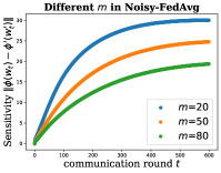
Sensitivity in Noisy-FedAvg. We mainly study the impact from the scale , local interval , and clipping norm , as shown in Fig. 2. The first figure clearly demonstrates the impact of the scale on sensitivity, which corresponds to the worst privacy bound . More clients generally imply stronger global privacy. The second figure shows evident that although increasing can raise the sensitivity during the process, it does not alter the upper bound of sensitivity after optimization converges. This is entirely consistent with our analysis, indicating that the privacy lower bound exists and is unaffected by and . The third figure indicates that the sensitivity will be affected by the , which corresponds to the worst privacy bound .
Sensitivity in Noisy-FedProx. We primarily explore the impact of the proximal coefficient and the comparison with Noisy-FedAvg. As shown in Fig. 2 (the fourth figure), the larger means smaller global sensitivity. This is consistent with our analysis, which states that the lower bound of privacy performance is given by . When we select , it degrades to the Noisy-FedAvg method. In fact, based on the comparison, we can see that when is sufficiently small, i.e. , its global sensitivity is almost at the same level as Noisy-FedAvg. In Table VII, we present a comparison between them. Although the proximal term provides limited improvement in accuracy, selecting an appropriate significantly reduces global sensitivity. This implies that the privacy performance of Noisy-FedProx is far superior to that of Noisy-FedAvg. While achieving similar performance, the regularization proxy term can significantly reduce the global sensitivity of the output model, thereby enhancing privacy. This conclusion also demonstrates the superiority on privacy of a series of FL-DP optimization methods based on training with this regularization approach, e.g. Noisy-FedADMM and several personalized FL-DP methods.
| Accuracy | Sensitivity | |
| Noisy-FedAvg | 60.67 | 31.33 |
| Noisy-FedProx | 60.69 | 30.97 |
| Noisy-FedProx | 60.94 | 18.52 |
| Noisy-FedProx | 56.33 | 6.34 |
VI Summary
To our best knowledge, this paper is the first work to demonstrate convergent privacy for the general FL-DP paradigms. We comprehensively study and illustrate the fine-grained privacy level for Noisy-FedAvg and Noisy-FedProx methods based on -DP analysis, an information-theoretic lossless DP definition. Moreover, we conduct comprehensive comparisons with existing work on other DP frameworks and highlight the long-term cognitive bias of the privacy lower bound regarding privacy budgets. Our analysis fills the theoretical gap in the convergent privacy of FL-DP while further providing a reliable theoretical guarantee for its privacy protection performance. Moreover, We conduct a series of experiments to verify the boundedness of global sensitivity and its influence on different variables, further validating that our theoretical analysis aligns more closely with practical scenarios.
References
- [1] B. McMahan, E. Moore, D. Ramage, S. Hampson, and B. A. y Arcas, “Communication-efficient learning of deep networks from decentralized data,” in Artificial intelligence and statistics. PMLR, 2017, pp. 1273–1282.
- [2] J. Geiping, H. Bauermeister, H. Dröge, and M. Moeller, “Inverting gradients-how easy is it to break privacy in federated learning?” Advances in neural information processing systems, vol. 33, pp. 16 937–16 947, 2020.
- [3] M. Nasr, R. Shokri, and A. Houmansadr, “Comprehensive privacy analysis of deep learning: Passive and active white-box inference attacks against centralized and federated learning,” in 2019 IEEE symposium on security and privacy (SP). IEEE, 2019, pp. 739–753.
- [4] C. Dwork, “Differential privacy,” in International colloquium on automata, languages, and programming. Springer, 2006, pp. 1–12.
- [5] C. Dwork, A. Roth et al., “The algorithmic foundations of differential privacy,” Foundations and Trends® in Theoretical Computer Science, vol. 9, no. 3–4, pp. 211–407, 2014.
- [6] M. Abadi, A. Chu, I. Goodfellow, H. B. McMahan, I. Mironov, K. Talwar, and L. Zhang, “Deep learning with differential privacy,” in Proceedings of the 2016 ACM SIGSAC conference on computer and communications security, 2016, pp. 308–318.
- [7] K. Wei, J. Li, M. Ding, C. Ma, H. H. Yang, F. Farokhi, S. Jin, T. Q. Quek, and H. V. Poor, “Federated learning with differential privacy: Algorithms and performance analysis,” IEEE transactions on information forensics and security, vol. 15, pp. 3454–3469, 2020.
- [8] R. Chourasia, J. Ye, and R. Shokri, “Differential privacy dynamics of langevin diffusion and noisy gradient descent,” Advances in Neural Information Processing Systems, vol. 34, pp. 14 771–14 781, 2021.
- [9] J. Ye and R. Shokri, “Differentially private learning needs hidden state (or much faster convergence),” Advances in Neural Information Processing Systems, vol. 35, pp. 703–715, 2022.
- [10] J. Altschuler and K. Talwar, “Privacy of noisy stochastic gradient descent: More iterations without more privacy loss,” Advances in Neural Information Processing Systems, vol. 35, pp. 3788–3800, 2022.
- [11] J. M. Altschuler, J. Bok, and K. Talwar, “On the privacy of noisy stochastic gradient descent for convex optimization,” SIAM Journal on Computing, vol. 53, no. 4, pp. 969–1001, 2024.
- [12] J. Dong, A. Roth, and W. J. Su, “Gaussian differential privacy,” Journal of the Royal Statistical Society: Series B (Statistical Methodology), vol. 84, no. 1, pp. 3–37, 2022.
- [13] J. Bok, W. Su, and J. M. Altschuler, “Shifted interpolation for differential privacy,” arXiv preprint arXiv:2403.00278, 2024.
- [14] L. Wasserman and S. Zhou, “A statistical framework for differential privacy,” Journal of the American Statistical Association, vol. 105, no. 489, pp. 375–389, 2010.
- [15] P. Kairouz, S. Oh, and P. Viswanath, “The composition theorem for differential privacy,” in International conference on machine learning. PMLR, 2015, pp. 1376–1385.
- [16] C. Dwork, A. Smith, T. Steinke, J. Ullman, and S. Vadhan, “Robust traceability from trace amounts,” in 2015 IEEE 56th Annual Symposium on Foundations of Computer Science. IEEE, 2015, pp. 650–669.
- [17] M. Hardt, B. Recht, and Y. Singer, “Train faster, generalize better: Stability of stochastic gradient descent,” in International conference on machine learning. PMLR, 2016, pp. 1225–1234.
- [18] I. Mironov, “Rényi differential privacy,” in 2017 IEEE 30th computer security foundations symposium (CSF). IEEE, 2017, pp. 263–275.
- [19] L. Shi, J. Shu, W. Zhang, and Y. Liu, “Hfl-dp: Hierarchical federated learning with differential privacy,” in 2021 IEEE Global Communications Conference (GLOBECOM). IEEE, 2021, pp. 1–7.
- [20] M. Zhang, E. Wei, and R. Berry, “Faithful edge federated learning: Scalability and privacy,” IEEE Journal on Selected Areas in Communications, vol. 39, no. 12, pp. 3790–3804, 2021.
- [21] M. Noble, A. Bellet, and A. Dieuleveut, “Differentially private federated learning on heterogeneous data,” in International Conference on Artificial Intelligence and Statistics. PMLR, 2022, pp. 10 110–10 145.
- [22] A. Cheng, P. Wang, X. S. Zhang, and J. Cheng, “Differentially private federated learning with local regularization and sparsification,” in Proceedings of the IEEE/CVF conference on computer vision and pattern recognition, 2022, pp. 10 122–10 131.
- [23] Y. Zhang and D. Tang, “A differential privacy federated learning framework for accelerating convergence,” in 2022 18th International Conference on Computational Intelligence and Security (CIS). IEEE, 2022, pp. 122–126.
- [24] R. Hu, Y. Guo, and Y. Gong, “Federated learning with sparsified model perturbation: Improving accuracy under client-level differential privacy,” IEEE Transactions on Mobile Computing, 2023.
- [25] T. Fukami, T. Murata, K. Niwa, and I. Tyou, “Dp-norm: Differential privacy primal-dual algorithm for decentralized federated learning,” IEEE Transactions on Information Forensics and Security, 2024.
- [26] N. Bastianello, C. Liu, and K. H. Johansson, “Enhancing privacy in federated learning through local training,” arXiv preprint arXiv:2403.17572, 2024.
- [27] S. P. Karimireddy, S. Kale, M. Mohri, S. Reddi, S. Stich, and A. T. Suresh, “Scaffold: Stochastic controlled averaging for federated learning,” in International conference on machine learning. PMLR, 2020, pp. 5132–5143.
- [28] T. Li, A. K. Sahu, M. Zaheer, M. Sanjabi, A. Talwalkar, and V. Smith, “Federated optimization in heterogeneous networks,” Proceedings of Machine learning and systems, vol. 2, pp. 429–450, 2020.
- [29] X. Zhang, M. Hong, S. Dhople, W. Yin, and Y. Liu, “Fedpd: A federated learning framework with adaptivity to non-iid data,” IEEE Transactions on Signal Processing, vol. 69, pp. 6055–6070, 2021.
- [30] S. U. Stich, “Local sgd converges fast and communicates little,” in ICLR 2019-International Conference on Learning Representations, 2019.
- [31] T. Lin, S. U. Stich, K. K. Patel, and M. Jaggi, “Don’t use large mini-batches, use local sgd,” in Proceedings of the 8th International Conference on Learning Representations, 2019.
- [32] B. Woodworth, K. K. Patel, S. Stich, Z. Dai, B. Bullins, B. Mcmahan, O. Shamir, and N. Srebro, “Is local sgd better than minibatch sgd?” in International Conference on Machine Learning. PMLR, 2020, pp. 10 334–10 343.
- [33] E. Gorbunov, F. Hanzely, and P. Richtárik, “Local sgd: Unified theory and new efficient methods,” in International Conference on Artificial Intelligence and Statistics. PMLR, 2021, pp. 3556–3564.
- [34] Y. Wang, Y. Tong, and D. Shi, “Federated latent dirichlet allocation: A local differential privacy based framework,” in Proceedings of the AAAI Conference on Artificial Intelligence, vol. 34, no. 04, 2020, pp. 6283–6290.
- [35] M. Chen, N. Shlezinger, H. V. Poor, Y. C. Eldar, and S. Cui, “Communication-efficient federated learning,” Proceedings of the National Academy of Sciences, vol. 118, no. 17, p. e2024789118, 2021.
- [36] P. Kairouz, H. B. McMahan, B. Avent, A. Bellet, M. Bennis, A. N. Bhagoji, K. Bonawitz, Z. Charles, G. Cormode, R. Cummings et al., “Advances and open problems in federated learning,” Foundations and trends® in machine learning, vol. 14, no. 1–2, pp. 1–210, 2021.
- [37] M. Mendieta, T. Yang, P. Wang, M. Lee, Z. Ding, and C. Chen, “Local learning matters: Rethinking data heterogeneity in federated learning,” in Proceedings of the IEEE/CVF Conference on Computer Vision and Pattern Recognition, 2022, pp. 8397–8406.
- [38] D. Jhunjhunwala, P. Sharma, A. Nagarkatti, and G. Joshi, “Fedvarp: Tackling the variance due to partial client participation in federated learning,” in Uncertainty in Artificial Intelligence. PMLR, 2022, pp. 906–916.
- [39] G. Malinovsky, K. Yi, and P. Richtárik, “Variance reduced proxskip: Algorithm, theory and application to federated learning,” Advances in Neural Information Processing Systems, vol. 35, pp. 15 176–15 189, 2022.
- [40] B. Li, M. N. Schmidt, T. S. Alstrøm, and S. U. Stich, “On the effectiveness of partial variance reduction in federated learning with heterogeneous data,” in Proceedings of the IEEE/CVF Conference on Computer Vision and Pattern Recognition, 2023, pp. 3964–3973.
- [41] H. Wang, S. Marella, and J. Anderson, “Fedadmm: A federated primal-dual algorithm allowing partial participation,” in 2022 IEEE 61st Conference on Decision and Control (CDC). IEEE, 2022, pp. 287–294.
- [42] Y. Sun, L. Shen, T. Huang, L. Ding, and D. Tao, “Fedspeed: Larger local interval, less communication round, and higher generalization accuracy,” arXiv preprint arXiv:2302.10429, 2023.
- [43] K. Mishchenko, G. Malinovsky, S. Stich, and P. Richtárik, “Proxskip: Yes! local gradient steps provably lead to communication acceleration! finally!” in International Conference on Machine Learning. PMLR, 2022, pp. 15 750–15 769.
- [44] M. Grudzień, G. Malinovsky, and P. Richtárik, “Can 5th generation local training methods support client sampling? yes!” in International Conference on Artificial Intelligence and Statistics. PMLR, 2023, pp. 1055–1092.
- [45] D. A. E. Acar, Y. Zhao, R. Matas, M. Mattina, P. Whatmough, and V. Saligrama, “Federated learning based on dynamic regularization,” in International Conference on Learning Representations.
- [46] Y. Sun, L. Shen, S. Chen, L. Ding, and D. Tao, “Dynamic regularized sharpness aware minimization in federated learning: Approaching global consistency and smooth landscape,” in International Conference on Machine Learning. PMLR, 2023, pp. 32 991–33 013.
- [47] W. Liu, L. Chen, Y. Chen, and W. Zhang, “Accelerating federated learning via momentum gradient descent,” IEEE Transactions on Parallel and Distributed Systems, vol. 31, no. 8, pp. 1754–1766, 2020.
- [48] P. Khanduri, P. Sharma, H. Yang, M. Hong, J. Liu, K. Rajawat, and P. Varshney, “Stem: A stochastic two-sided momentum algorithm achieving near-optimal sample and communication complexities for federated learning,” Advances in Neural Information Processing Systems, vol. 34, pp. 6050–6061, 2021.
- [49] R. Das, A. Acharya, A. Hashemi, S. Sanghavi, I. S. Dhillon, and U. Topcu, “Faster non-convex federated learning via global and local momentum,” in Uncertainty in Artificial Intelligence. PMLR, 2022, pp. 496–506.
- [50] Y. Sun, L. Shen, H. Sun, L. Ding, and D. Tao, “Efficient federated learning via local adaptive amended optimizer with linear speedup,” IEEE Transactions on Pattern Analysis and Machine Intelligence, vol. 45, no. 12, pp. 14 453–14 464, 2023.
- [51] Y. Sun, L. Shen, and D. Tao, “Understanding how consistency works in federated learning via stage-wise relaxed initialization,” Advances in Neural Information Processing Systems, vol. 36, 2024.
- [52] A. Reisizadeh, A. Mokhtari, H. Hassani, A. Jadbabaie, and R. Pedarsani, “Fedpaq: A communication-efficient federated learning method with periodic averaging and quantization,” in International conference on artificial intelligence and statistics. PMLR, 2020, pp. 2021–2031.
- [53] N. Shlezinger, M. Chen, Y. C. Eldar, H. V. Poor, and S. Cui, “Uveqfed: Universal vector quantization for federated learning,” IEEE Transactions on Signal Processing, vol. 69, pp. 500–514, 2020.
- [54] R. Dai, L. Shen, F. He, X. Tian, and D. Tao, “Dispfl: Towards communication-efficient personalized federated learning via decentralized sparse training,” in International conference on machine learning. PMLR, 2022, pp. 4587–4604.
- [55] X. Yao, T. Huang, C. Wu, R. Zhang, and L. Sun, “Towards faster and better federated learning: A feature fusion approach,” in 2019 IEEE International Conference on Image Processing (ICIP). IEEE, 2019, pp. 175–179.
- [56] L. Zhang, Y. Luo, Y. Bai, B. Du, and L.-Y. Duan, “Federated learning for non-iid data via unified feature learning and optimization objective alignment,” in Proceedings of the IEEE/CVF international conference on computer vision, 2021, pp. 4420–4428.
- [57] J. Xu, X. Tong, and S.-L. Huang, “Personalized federated learning with feature alignment and classifier collaboration,” in The Eleventh International Conference on Learning Representations.
- [58] C. Dwork, F. McSherry, K. Nissim, and A. Smith, “Calibrating noise to sensitivity in private data analysis,” in Theory of Cryptography: Third Theory of Cryptography Conference, TCC 2006, New York, NY, USA, March 4-7, 2006. Proceedings 3. Springer, 2006, pp. 265–284.
- [59] C. Dwork, K. Kenthapadi, F. McSherry, I. Mironov, and M. Naor, “Our data, ourselves: Privacy via distributed noise generation,” in Advances in Cryptology-EUROCRYPT 2006: 24th Annual International Conference on the Theory and Applications of Cryptographic Techniques, St. Petersburg, Russia, May 28-June 1, 2006. Proceedings 25. Springer, 2006, pp. 486–503.
- [60] J. Zhao, Y. Chen, and W. Zhang, “Differential privacy preservation in deep learning: Challenges, opportunities and solutions,” IEEE Access, vol. 7, pp. 48 901–48 911, 2019.
- [61] P. C. M. Arachchige, P. Bertok, I. Khalil, D. Liu, S. Camtepe, and M. Atiquzzaman, “Local differential privacy for deep learning,” IEEE Internet of Things Journal, vol. 7, no. 7, pp. 5827–5842, 2019.
- [62] J. Wu, W. Hu, H. Xiong, J. Huan, V. Braverman, and Z. Zhu, “On the noisy gradient descent that generalizes as sgd,” in International Conference on Machine Learning. PMLR, 2020, pp. 10 367–10 376.
- [63] M. Bun and T. Steinke, “Concentrated differential privacy: Simplifications, extensions, and lower bounds,” in Theory of cryptography conference. Springer, 2016, pp. 635–658.
- [64] M. Bun, C. Dwork, G. N. Rothblum, and T. Steinke, “Composable and versatile privacy via truncated cdp,” in Proceedings of the 50th Annual ACM SIGACT Symposium on Theory of Computing, 2018, pp. 74–86.
- [65] R. C. Geyer, T. Klein, and M. Nabi, “Differentially private federated learning: A client level perspective,” arXiv preprint arXiv:1712.07557, 2017.
- [66] L. Zhu, X. Liu, Y. Li, X. Yang, S.-T. Xia, and R. Lu, “A fine-grained differentially private federated learning against leakage from gradients,” IEEE Internet of Things Journal, vol. 9, no. 13, pp. 11 500–11 512, 2021.
- [67] A. Lowy, A. Ghafelebashi, and M. Razaviyayn, “Private non-convex federated learning without a trusted server,” in International Conference on Artificial Intelligence and Statistics. PMLR, 2023, pp. 5749–5786.
- [68] X. Yang and W. Wu, “A federated learning differential privacy algorithm for non-gaussian heterogeneous data,” Scientific Reports, vol. 13, no. 1, p. 5819, 2023.
- [69] R. Hu, Y. Guo, H. Li, Q. Pei, and Y. Gong, “Personalized federated learning with differential privacy,” IEEE Internet of Things Journal, vol. 7, no. 10, pp. 9530–9539, 2020.
- [70] G. Yang, S. Wang, and H. Wang, “Federated learning with personalized local differential privacy,” in 2021 IEEE 6th International Conference on Computer and Communication Systems (ICCCS). IEEE, 2021, pp. 484–489.
- [71] X. Yang, W. Huang, and M. Ye, “Dynamic personalized federated learning with adaptive differential privacy,” Advances in Neural Information Processing Systems, vol. 36, pp. 72 181–72 192, 2023.
- [72] K. Wei, J. Li, C. Ma, M. Ding, W. Chen, J. Wu, M. Tao, and H. V. Poor, “Personalized federated learning with differential privacy and convergence guarantee,” IEEE Transactions on Information Forensics and Security, 2023.
- [73] T. Wittkopp and A. Acker, “Decentralized federated learning preserves model and data privacy,” in International Conference on Service-Oriented Computing. Springer, 2020, pp. 176–187.
- [74] S. Chen, D. Yu, Y. Zou, J. Yu, and X. Cheng, “Decentralized wireless federated learning with differential privacy,” IEEE Transactions on Industrial Informatics, vol. 18, no. 9, pp. 6273–6282, 2022.
- [75] Y. Gao, L. Zhang, L. Wang, K.-K. R. Choo, and R. Zhang, “Privacy-preserving and reliable decentralized federated learning,” IEEE Transactions on Services Computing, vol. 16, no. 4, pp. 2879–2891, 2023.
- [76] Y. Shi, Y. Liu, K. Wei, L. Shen, X. Wang, and D. Tao, “Make landscape flatter in differentially private federated learning,” in Proceedings of the IEEE/CVF Conference on Computer Vision and Pattern Recognition, 2023, pp. 24 552–24 562.
- [77] A. Girgis, D. Data, S. Diggavi, P. Kairouz, and A. T. Suresh, “Shuffled model of differential privacy in federated learning,” in International Conference on Artificial Intelligence and Statistics. PMLR, 2021, pp. 2521–2529.
- [78] X. Wu, Y. Zhang, M. Shi, P. Li, R. Li, and N. N. Xiong, “An adaptive federated learning scheme with differential privacy preserving,” Future Generation Computer Systems, vol. 127, pp. 362–372, 2022.
- [79] Z. He, L. Wang, and Z. Cai, “Clustered federated learning with adaptive local differential privacy on heterogeneous iot data,” IEEE Internet of Things Journal, 2023.
- [80] N. Rodríguez-Barroso, G. Stipcich, D. Jiménez-López, J. A. Ruiz-Millán, E. Martínez-Cámara, G. González-Seco, M. V. Luzón, M. A. Veganzones, and F. Herrera, “Federated learning and differential privacy: Software tools analysis, the sherpa. ai fl framework and methodological guidelines for preserving data privacy,” Information Fusion, vol. 64, pp. 270–292, 2020.
- [81] K. Wei, J. Li, M. Ding, C. Ma, H. Su, B. Zhang, and H. V. Poor, “User-level privacy-preserving federated learning: Analysis and performance optimization,” IEEE Transactions on Mobile Computing, vol. 21, no. 9, pp. 3388–3401, 2021.
- [82] M. Kim, O. Günlü, and R. F. Schaefer, “Federated learning with local differential privacy: Trade-offs between privacy, utility, and communication,” in ICASSP 2021-2021 IEEE International Conference on Acoustics, Speech and Signal Processing (ICASSP). IEEE, 2021, pp. 2650–2654.
- [83] Q. Zheng, S. Chen, Q. Long, and W. Su, “Federated f-differential privacy,” in International conference on artificial intelligence and statistics. PMLR, 2021, pp. 2251–2259.
- [84] J. Ling, J. Zheng, and J. Chen, “Efficient federated learning privacy preservation method with heterogeneous differential privacy,” Computers & Security, vol. 139, p. 103715, 2024.
- [85] S. Jiao, L. Cai, X. Wang, K. Cheng, and X. Gao, “A differential privacy federated learning scheme based on adaptive gaussian noise.” CMES-Computer Modeling in Engineering & Sciences, vol. 138, no. 2, 2024.
- [86] Y. LeCun, L. Bottou, Y. Bengio, and P. Haffner, “Gradient-based learning applied to document recognition,” Proceedings of the IEEE, vol. 86, no. 11, pp. 2278–2324, 1998.
- [87] A. Krizhevsky, G. Hinton et al., “Learning multiple layers of features from tiny images,” 2009.
- [88] K. He, X. Zhang, S. Ren, and J. Sun, “Deep residual learning for image recognition,” in Proceedings of the IEEE conference on computer vision and pattern recognition, 2016, pp. 770–778.
[Proof of Main Theorems]
A.1 Proofs of Eq. (12)
We consider the general updates on the adjacent datasets and on round as follows:
| (25) |
where is the initial state. and are two noises generated from the normal distribution . To construct the interpolated sequence, we introduce the concentration coefficients to provide a convex combination of the updates above, which is,
| (26) |
for . Furthermore, we set to let , and we add the definition of as the interpolation beginning. determines the length of the interpolation sequence.
Lemma 5 (Lemma 3.2 and C.4 in [13]).
According to the expansion of trade-off functions, for the general updates in Eq.(26), we have the following recurrence relation:
| (27) |
Proof.
Based on the post-processing and compositions, let and be the corresponding noises above, for any constant , we have (subscripts are temporarily omitted):
where and are two Gaussian noises that can be considered to be sampled from (average of isotropic Gaussian noises). Therefore, the distinguishability between the first term and the second term does not exceed the mean shift of the distribution, which is . By taking and , the proofs are completed.
∎
According to the above lemma, by expanding it from to and the factor , we can prove the formulation in Eq. (12).
A.2 Proofs of Theorem 1
Lemma 5 provides the general recursive relationship on the global states along the communication round . To obtain the lower bound of the trade-off function, we only need to solve for the gaps . It is worth noting that the local update process here involves dual replacement of both the dataset ( and ) and the initial state ( and ). Therefore, we measure their maximum discrepancy by assessing their respective distances to the intermediate variable constructed by the cross-items:
| (28) |
The first term measures the disparity in training on different datasets and the second term measures the gap in training from different initial models. One of our contributions is to provide their general gaps. In [13], it only considers the strongly convex and general convex objectives under one local iteration. In our paper, we expand the update function by considering the multiple local iterations and federated cross-device settings. By simply setting the local interval to and the number of clients to , our results can easily reproduce the original conclusion in [13]. Furthermore, our comprehensive considerations have led to a new understanding of the impact of local updates on privacy.
To explain these two terms more intuitively, we sketch the processes of , , and in Fig. (1), to further illustrate their differences. and begin from . and adopt the data samples . We naturally use and to represent individual states in and , respectively. To avoid ambiguity, we define the states in as . When , since , then only differs from on -th client.
on the Noisy-FedAvg Method:
Lemma 6 (Data Sensitivity.).
The data sensitivity caused by gradient descent steps can be bounded as:
| (29) |
where is the learning rate at the -th iteration of -th communication round.
Proof.
By directly expanding the update functions and at , we have:
The last equation adopts when . This completes the proofs. ∎
Lemma 7 (Model Sensitivity.).
The model sensitivity caused by gradient descent steps can be bounded as:
| (30) |
where is a constant related the selection of learning rates.
Proof.
We first learn an individual case. On the -th round, we assume the initial states of two sequences are and . Each is performed by the update function for local steps. For each step, we have:
This implies each gap when can be upper bounded by:
Then we consider the recursive formulation of the stability gaps along the iterations . We can directly apply Eq.(26) to obtain the relationship for the differences updated from different initial states on the same dataset. By directly expanding the update function at and , we have:
This completes the proofs.
∎
We have successfully quantified the specific form of the problem as above. By solving for a series of reasonable values of the auxiliary variable to minimize the above problem, we obtain the tight lower bound on privacy. Before that, let’s discuss the learning rate to simplify this expression. Both and terms are highly related to the selections of learning rates. Typically, this choice is determined by the optimization process. Whether it’s generalization or privacy analysis, both are based on the assumption that the optimization can converge properly. Therefore, we selected several different learning rate designs based on various combination methods to complete the subsequent analysis. Due to the unique two-stage learning perspective of federated learning, current methods for designing the learning rate generally choose between a constant rate or a rate that decreases with local rounds or iterations. Therefore, we discuss them separately including constant learning rate, cyclically decaying learning rate, stage-wise decaying learning rate, and continuously decaying learning rate. We provide a simple comparison in Figure 3.


Constant learning rates
This is currently the simplest case. We consider the learning rate to always be a constant, i.e. . Then we have that the accumulation term . For the term, we have:
When is selected, both of them can be considered as a constant related to . The choice of also requires careful consideration. Although it is a constant, its selection is typically related to , , and based on the optimization process. We will discuss this point in the final theorems.
Cyclically decaying learning rates
Some works treat this learning process as an aggregation process of several local training processes, i.e. each local client learns from a better initial state (knowledge learned from other clients). And since the client pool is very large, most clients will exit after obtaining the model they desire. This setting is often used in “cross-device” scenarios [36]. Thus, local learning can be considered as an independent learning process. In this case, the learning rate is designed to decay in an inversely proportional function to achieve optimal local accuracy, i.e. , and is restored to a larger initial value at the start of each round, i.e. . Then we have the accumulation term:
| (31) |
When is large, this term is dominated by . Based on the fact that is very large in federated learning, we further approximate this term to where is a scaled constant. It is easy to check that there must exist for any . Thus we have the accumulation term as . For the term, we have its upper bound:
The first inequality adopts and the last adopts the concavity. Actually, we still can learn its general lower bound by a scaling constant. By adopting a scaling , we can have , which is equal to . It is also easy to check when . Thus we have:
The last inequality also adopts concavity. Through this simple scaling, we learn the general bounds for the learning rate function as:
| (32) |
where , and (this condition is almost universally satisfied in current optimization theories). Although we cannot precisely find the tight bound of this function , we can still treat it as a form based on constants to complete the subsequent analysis, i.e. it could be approximated as a larger upper bound . More importantly, we have determined that this learning rate function still diverges as increases.
Stage-wise decaying learning rates
This is one of the most common selections of learning rate in the current federated community, which is commonly applied in “cross-silo” scenarios [36]. When the client pool is not very large, clients who participate in the training often aim to establish long-term cooperation to continuously improve their models. Therefore, each client will contribute to the entire training process over a long period. From a learning perspective, local training is more like exploring the path to a local optimum rather than actually achieving the local optimum. Therefore, each local training will adopt a constant learning rate and perform several update steps, i.e. . At each communication round, the learning rate decays once and continues to the next stage, i.e. . Based on the analysis of the constant learning rate, the accumulation term is . For the term, we have:
It can be seen that the analysis of this function is more challenging because the learning rate function is decided by , which introduces complexity to the subsequent analysis. We will explain this in detail in the subsequent discussion.
Continuously decaying learning rates
This is a common selection of learning rate in the federated community, involving dual learning rate decay along both local training and global training. This can almost be applied to all methods to adapt to the final training, including both the cross-silo and cross-device cases. At the same time, its analysis is also more challenging because the learning rate is coupled with communication rounds and local iterations, yielding new upper and lower bounds. We consider the general case . Therefore, the accumulation term can be bounded as:
Similarly, when is large enough, this term is dominated by . For simplicity in the subsequent proof, we follow the process above and let it be to include the term at . It is also easy to check that is a constant for any . And is also a constant. It means we can always select the lower bound as its representation. Therefore, for the learning rate function , we have:
Similarly, we introduce the coefficient to provide the lower bound as:
Through the sample scaling, we learn the general bounds for the learning rate function as:
| (33) |
where , and .
Obviously, when is large enough, the learning rate term is still dominated by . Therefore, to learn the general cases, we can consider the specific form of the learning rate function based on the constant scaling as . As increases, this function will approach zero.
on the Noisy-FedProx Method:
In this part, we will address the differential privacy analysis of a noisy version of another classical federated learning optimization method, i.e. the Noisy-FedProx method. The vanilla FedProx method is an optimization algorithm designed for cross-silo federated learning, particularly to address the challenges caused by data heterogeneity across different clients. Unlike traditional federated learning algorithms like FedAvg, which can struggle with variations in data distribution, it introduces a proximal term to the objective function. This helps to stabilize the training process and improve convergence. Specifically, it adopts the consistency as the penalized term to correct the local objective:
| (34) |
The proximal term is a very common regularization term in federated learning and has been widely used in both federated learning and personalized federated learning approaches. It introduces an additional penalty to the local objective, ensuring that local updates are optimized towards the local optimal solution while being subject to an extra global constraint, i.e. each local update does not stray too far from the initialization point. In fact, there are many optimization methods that apply such regularization terms. For example, various federated primal-dual methods based on the ADMM approach construct local Lagrangian functions, and in personalized federated learning, local privatization regularization terms are introduced to differentiate from the vanilla consistency objective. The analysis of the above methods is fundamentally based on a correct understanding of the advantages and significance of the proximal term in stability error. In this paper, to achieve a cross-comparison while maintaining generality, we consider the optimization process of local training as total -step updates:
| (35) |
Here, we also employ the proofs mentioned in the previous section, and our study of the difference term is based on both data sensitivity and model sensitivity perspectives. We provide these two main lemmas as follows.
Lemma 8 (Data Sensitivity.).
The local data sensitivity of the Noisy-FedProx method at -th communication round can be upper bounded as:
| (36) |
Proof.
We first consider a single step in Eq.(35) as:
The proximal term brings more opportunities to enhance the analysis of local updates. We can split the proximal term and subtract the term on both sides, resulting in a recursive formula for the cumulative update term:
The above equation indicates that a reduction factor can limit the scale of local updates. This is a very good property, allowing us to shift the analysis of the data sensitivity to their relationship of local updates. According to the above, we can upper bound the gaps between and sequences as:
Different from proofs in Lemma 6, the term can further decrease the stability gap during accumulation. By summing form to , we can obtain:
Here, we provide a simple proof using a constant learning rate to demonstrate that its upper bound can be independent of . By considering , we have:
In fact, when the learning rate decays with , it can still be easily proven to have a constant upper bound. Therefore, in the subsequent proofs, we directly use the form of this constant upper bound as the result of data sensitivity in the Noisy-FedProx method. Based on the definition of , we have:
This completes the proofs. ∎
Lemma 9 (Model Sensitivity.).
The local model sensitivity of the Noisy-FedProx method at -th communication round can be upper bounded as:
| (37) |
Proof.
We also adopt the splitting above. Since both sequences are trained on the same dataset, the gradient difference can be measured by the parameter difference. Therefore, we directly consider the form of the parameter difference:
where is a constant. Here, we consider . When , its upper bound can not be guaranteed to be reduced. When , it can restore the property of decayed stability. By summing from to , we can obtain:
Similarly, we learn the upper bound from a simple constant learning rate. By select , we have:
The same, it can also be checked that the general upper bound of the stability gaps is a constant even if the learning rate is selected to be decayed along iteration . Therefore, in the subsequent proofs, we directly use the form of this constant upper bound as the result of model sensitivity in the Noisy-FedProx method. Based on the definition of , we have:
This completes the proofs. ∎
A.3 Solution of Eq. (15)
According to the recurrence relation in Lemma 5, we can confine the privacy amplification process to a finite number of steps with the aid of an interpolation sequence, yielding to the convergent bound. Therefore, we have:
Although the above form appears promising, an inappropriate selection of the key parameters will still cause divergence due to the recurrence term coefficient , leading it to approach infinity as increases. For instance, small will result in a significantly increased and the bound will be closed to the stability gap , and large will result in a long accumulation of the stability gaps, which is also unsatisfied. At the same time, it is also crucial to choose appropriate to ensure that the stability accumulation can be reasonably diluted. Therefore, we also need to thoroughly investigate how significant the stability gap caused by the interpolation points is. According to Eq.(25) and (26), we have:
The above relationship further constrains the stability of the interpolation sequence. It is worth noting that the upper bound of the final step is independent of the choice of . At the same time, since all terms are positive, given a group of specific , taking the upper bound at each possible will result in the maximum error accumulation. This is also the worst-case privacy we have constructed. Therefore, solving the worst privacy could be considered as solving the following problem:
| (38) |
Based on the above analysis, this problem can be directly transformed into a privacy minimization problem when the interpolation sequence reaches the maximum stability error. Therefore, we just need to solve the following problem:
| (39) |
It is important to note that this upper bound condition is usually loose because the probability that the interpolation terms simultaneously reach their maximum deviation is very low. This is merely the theoretical worst-case privacy scenario.
Then we solve the minimization problem. By considering the worst stability conditions, we can provide the relationship between the gaps and coefficients as:
Expanding it from to , we have:
Due to the term being part of the analytical form of the minimization objective, we preserve the integrity of this algebraic form and only split it from the perspectives of coefficients , and . According to the definition , then we have:
| (40) |
The above equation presents the summation of the term accompanied by a scaling coefficient . It naturally transforms the summation form into an initial stability gap and a constant term achieved through a combination of learning rates. To solve it, we can directly adopt the Cauchy-Schwarz inequality to separate the terms and construct a constant term based on the form of the scaling coefficient to find its achievable lower bound:
Although the original problem requires solving the , here we can know one possible minimum form of the problem no longer includes this parameter. In fact, this parameter has been transformed into the optimality condition of the Cauchy-Schwarz inequality, which is given by
| (41) |
where is a positive constant. We will discuss the value of and the validity of the optimality conditions in detail in the final conclusions.
Therefore, we only need to optimize it w.r.t the parameter . Unfortunately, this part highly correlates with the stability gaps . Current research progress indicates that in non-convex optimization, this term diverges as the number of training rounds increases. This makes it difficult for us to accurately quantify its specific impact on the privacy bound. If is very small, it means that the introduced stability gap will also be very small. However, consequently, the coefficients of the and terms will increase due to the accumulation over rounds. To detail this, we have to make certain compromises. Because is an integer belonging to , we denote its optimal selection by (it certainly exists when is given). Therefore, the privacy lower bound under other choices of will certainly be more relaxed, i.e. (privacy is weak at other selection of ). This allows us to look for other asymptotic solutions instead of finding the optimal solution. Although we cannot ultimately achieve the form of the optimal solution, we can still provide a stable privacy lower bound. To eliminate the impact of stability error, we directly choose , yielding the following bound:
By substituting the values of and under different cases, then we can prove the main theorems in this paper.