A novel numerical framework for three-dimensional fully resolved simulation of freely falling particles of arbitrary shape

Abstract

This article introduces a novel numerical framework designed to model the interplay between free-falling particles and their surrounding fluid in situations of high particle to fluid density ratio, typically exhibited by atmospheric particles. This method is designed to complement experimental studies in vertical wind tunnels to improve the understanding of the aerodynamic behavior of small atmospheric particles, such as the transport and sedimentation of volcanic particles, cloud ice crystals and other application areas. The solver is based on the lattice Boltzmann method and it addresses the numerical challenges, including the high density ratio and moderate to high Reynolds number, by using an immersed-boundary approach and a recursive-regularized collision model. A predictor-corrector scheme is applied for the robust time integration of the six-degrees-of-freedom (6DOF) rigid-body motion. Finally, the multi-scale nature arising from the long free-fall distances of a particle is addressed through a dynamic memory allocation scheme allowing for a virtually infinite falling distance. This tool allows for the simulation of particles of arbitrary shape represented by a triangularized surface. The framework is validated against the analytical and experimental data for falling spheres and ellipsoids, and is then applied to the case of an actual volcanic particle geometry, the shape of which is obtained from a 3D surface-contour scanning process. The physics of the free-fall of this particle is investigated and described, and its terminal velocity is compared against the experimental data measured with the 3D printed exemplars of the same particle.

1 Introduction

Particles moving in fluids are ubiquitous, from indoor air to the atmosphere and ocean to technical applications. With a few exceptions, such as small water droplets [1], such particles are almost universally non-spherical. Examples of such particles are volcanic ash [2], dust [3], pollen [4], ice crystals [5], marine snow [6] and microplastics [7], which mostly range in size from a few tens of micrometres to several centimetres (for the sake of brevity we exclude very small and large particles here). Their dynamics are influenced by their material properties such as density, size and shape, as well as by the properties of the ambient fluid and the flow characteristics. There is a long list of theoretical, experimental and numerical studies in the literature dealing with this topic [8, 9, 10, 11, 12, 13, 14, 15, 16, 17]. While experimental studies can provide the ground truth to guide and validate models, a reliable simulation can provide much more information about the particle dynamics that is not achievable in experiments. In recent years, several numerical methods have been proposed, which have demonstrated their capability in capturing some of the essential physical phenomena of such processes with high efficiency and accuracy [18, 19, 20, 21, 22].

The methods commonly rely on an immersed-particle philosophy, in which the fluid mesh is stationary, and mesh points are allocated both outside and inside the particle. The common implementations of this philosophy are the saturated-cell approach, which relies on a computation of the solid fraction across the interface of the moving particle [23, 24], or the immersed-boundary approach [19, 21], which simulates a fluid equation inside the solid as well. Both approaches avoid the need for costly remeshing of the fluid domain surrounding the moving particles. In this work, we focus on the immersed-boundary approach as one of the two common options in the Lattice Boltzmann modeling of rigid solid motion.

If the particle is considered rigid, its time evolution can be described by a model with six-degrees-of-freedom, or ‘6DOF’ for short, corresponding to three degrees of freedom for the position and three degrees of freedom for the orientation [25]. The resolution of the equations of motion relies on the computation of the total force and moment-of-force, which is obtained by integrating over an arbitrary particle shape [26].

A numerical framework is generally tailored for specific Reynolds numbers and particle to fluid density ratio regimes. Abundant literature exists for numerical simulation of particle suspensions at low Reynolds numbers and with density ratios close to 1 [27, 28, 29, 30]. These simulations have wide-ranging applications including sedimentation processes for particles immersed in fluids, where the particle density places them in a close-to-buoyant regime. To name another example, numerical simulation has made significant progress in representing blood components, including red blood cells or platelets, at the cellular level for biomedical process descriptions [31, 32, 33]. In such cases, the use of a solver capable of complete fluid-structure interaction is necessary due to the deformable nature of the blood cells.

The particle dynamics is usually characterised by the Reynolds number of the particles $\mathrm{Re}_{T}=v_{\mathrm{T}}d/\nu$, which is defined as the relative velocity of the particles (here terminal velocity $v_{\mathrm{T}}$) multiplied by a characteristic length of the particles (here particle diameter $d$) and divided by the kinematic viscosity of the fluid $\nu$. In a turbulent flow, other dimensionless parameters also play a role. However, even in a laminar flow, it is not only the Reynolds number of the particles that is important, but also the ratio of the particle density to the fluid density. It has already been shown that for a Reynolds number $>$ 100, the terminal velocity increases with the density ratio [11, 15]. Recently, it was also found that the angular dynamics of particles with Reynolds number between 1-10 is also significantly influenced by the density ratio [17].

One of the main difficulties in the experimental or numerical study of free-falling particles is their multi-scale nature. Length scales range from the size of the particles, e.g. a few hundred micrometres to centimetres, to drop distances that are ten or a thousand times the particle size to reach terminal velocity when a stable orientation is present or to collect sufficient statistics on the pseudo-terminal settling velocity of the particles when no stable orientation is present. Together with the need for high resolution to correctly resolve the shape features of the particles and the particle-fluid interactions, this problem can be fundamentally intractable given current computational power. A typical workaround calls for the limitation of the effective numerical domain size, but the close proximity to a no-slip wall representing the immutable reference frame (the ground) can in this case cause follow-up numerical and physical errors.

We introduce in this work a novel numerical framework to model particle free-fall that addresses these issues. The framework is an extension of the Palabos library [34], a general-purpose computational fluid dynamics (CFD) code with a kernel based on the Lattice-Boltzmann method (LBM). The numerical stability of the flow is improved using the recursive-regularized collision model [35, 36]. This model also includes a subgrid-scale filtering capability achieved by projecting kinetic variables onto a Hermite-tensor subspace. This collision model therefore not only maintains stability but also ensures sufficient accuracy during local direct numerical simulation (DNS) to large-eddy simulation (LES) transition, which is expected to take place frequently in this flow regime. As demonstrated in this study, this LBM allows for the retrieval of fluid flow values with high precision to determine the force and moment of force acting on the surface of the immersed particle.

Owing to the adopted velocity discretization scheme, the LBM is traditionally limited to the use of structured meshes with uniform, cubic cells. Although this limitation is in practice overcome using mesh refinement on a hierarchic, octree-like mesh structure, such an extension is not used in the present work, which makes use of a fully uniform mesh. One of the consequences of the uniform mesh structure is that the mesh is not body-fitted for any object that has a non-rectangular shape or is moving.

As a workaround, the LBM community has a well-established set of tools for accurately resolving boundary conditions for moving, immersed objects. Earlier methods, which were developed by Hu (1992) [37], Feng et al. (1994) [38, 39], Ladd (1994) [40, 41], Aidun (1995) [42], and Johnson (1995) [43], applied a staircased pattern to represent a particle boundary that followed the shape of the fluid solver’s mesh. They required a large particle size compared to the computational grid or mesh spacing to achieve stable and consistent results, or they needed to frequently remesh the fluid domain around the moving particles. Recently, a significant amount of research has been conducted to expand both conventional CFD approaches and the LBM in order to achieve a more precise representation of the surfaces of moving particles in fluids, without increasing the resolution of the computational domain [44, 45, 46, 47, 48, 49, 50, 51, 52, 53, 54]. In separate research endeavors, the LBM has developed the ability to accurately represent curved boundaries over time [55].

In this paper, we concentrate on a multi-directional forcing technique that has was adapted for the LBM. In a research effort related to the present one, this approach has previously been used to model particles with density ratios close to unity [56]. The present work extends this framework to high density ratios and to particles of arbitrary shape. For this, the boundary representation is complemented with a time-integration scheme for the 6DOF of a rigid particle, leading to a complete computational framework for immersed particle motion, which is implemented in the LBM software library Palabos [34].

The paper is divided into two parts. The first part outlines the computational framework for the particle free-fall experiment, which includes the recursive-regularized LBM for the fluid equations, the immersed boundary condition for the fluid-particle coupling, and a time-staggered predictor-corrector method for the time integration of the particle motion. To allow for a long free-fall distance without spending an excessive amount of memory, a dynamic memory allocation strategy is utilized. It involves a gradual removal of domains from the particle’s far wake and the addition of domains up front, permitting for the particle trajectory to be extended as often as necessary. The validity of the framework is confirmed in two simple cases, the time-dependent behavior of a sphere experiencing rotation-free free-fall and a displacement-free rotational motion. In the second part, the proposed numerical framework is used to investigate different scenarios with falling particles, such as spheroidal and irregular volcanic (lapilli-size) particles in a wide range of Reynolds number $\sim$ 5 - 10000 and a particle-to-fluid density ratio of $\sim$ 1000. The results are then compared with experimental measurements performed with the Göttingen Turret [17] and the UNIGE Vertical Wind Tunnel [57]. The numerical results show a high degree of agreement with the experimental observations, validating the numerical code.

2 Numerical method

2.1 Lattice Boltzmann method (LBM)

In the present work, the air is modeled as an incompressible fluid, as governed by the incompressible Navier-Stokes equations:

$$\partial_{t}{\bm{u}}+\left({\bm{u}}\cdot{\bm{\nabla}}\right){\bm{u}} =-{\bm{\nabla}}p+\nu\nabla^{2}{\bm{u}}\quad\mathrm{and}$$ (1)

$${\bm{\nabla}}\cdot{\bm{u}} =0,$$ (2)

where $\bm{u}$ is the flow velocity, $p$ is the fluid pressure divided by the fluid density $\rho_{\mathrm{f}}$, and $\nu$ is the kinematic viscosity of the fluid. The LBM is a solver for the Boltzmann equation which, for the present problem, runs as a quasi-compressible solver to find solutions to the above equations.

The primitive variables in the LBM are the so-called particle populations $f_{i}(\bm{x},t)$, which represent a discretized version of the distribution function $f(\bm{x},\bm{\xi},t)$:

$$f_{i}(\bm{x},t)\equiv f(\bm{x},\bm{\xi}_{i},t),$$ (3)

where the index $i=0,\cdots,q-1$ identifies the elements of a discretized velocity space $\{\bm{\xi}_{i}\}_{i=0}^{q-1}$. The properties of the numerical model depend among others on the choice of discrete velocities. In the present work, we choose the 27-velocity model, D3Q27 lattice [58], which appears to show better numerical stability for the present problem than the commonly used D3Q19 lattice. The details of the 27 discrete velocities are stated as

$$\{\bm{\xi}_{i}\}=\left\{\frac{\delta x}{\delta t}(k{\bm{e}}_{0}+l{\bm{e}}_{1}+m{\bm{e}}_{2}),\quad k=0\cdots 2,\quad l=0\cdots 2,\quad m=0\cdots 2\right\},$$ (4)

where $\delta x$ and $\delta t$ are the spatial and temporal resolutions respectively, and ${\bm{e}}_{0}$, ${\bm{e}}_{1}$, ${\bm{e}}_{2}$ are the Cartesian basis vectors.

The macroscopic variables, pressure $p$ and velocity $\bm{u}$, are moments of the distribution function, and in the discrete case can be expressed through weighted sums of the particle populations:

$$p =c_{s}^{2}\left(\sum_{i}f_{i}-\rho_{0}\right),$$ (5)

$$\bm{u} =\frac{\sum_{i}\bm{\xi}_{i}f_{i}}{\sum_{i}f_{i}}.$$ (6)

In the present quasi-compressible approach, the constants $c_{s}$ and $\rho_{0}$ have a purely numerical meaning, and take the value $c_{s}^{2}=1/3\,\delta x^{2}/\delta t^{2}$ and $\rho_{0}=1$.

Lattice Boltzmann models usually approximate the collision term by a perturbation around an equilibrium value, described by the Maxwell-Boltzmann distribution. This function depends on the macroscopic variables, such as, velocity and pressure, and is most often approximated by a polynomial of a given degree, which is constructed in a way to reproduce the selected velocity moments exactly. In this work, we select a fourth-order equilibrium term and model the collision with the recursive-regularized approach presented in [59], which is a more robust variation of the classical BGK algorithm (for Bhatnagar, Gross, and Krook, see [60]). The evolution rule reads

$$f_{i}(\bm{x}+\bm{\xi}_{i}\delta t,t+\delta t)=f^{(0)}_{i}(p,\bm{u})+\left(1-\frac{1}{\tau}\right)f^{(1)}_{i},$$ (7)

where $f^{(0)}_{i}$ is the equilibrium population, expanded to fourth order with respect to the Mach number, as detailed in A. The off-equilibrium population $f^{(1)}_{i}$, also detailed in A, is projected onto a sub-space spanned by Hermite tensor polynomials, to filter out high-frequency fluctuations (see [59] for further details). Consequently, the under-resolved, turbulent simulations presented in this article are run without any LES-type turbulence model, as subgrid scales are filtered by the collision model. The variable $\tau$ represents the relaxation time. The Chapman–Enskog expansion (see [61]) relates the relaxation time to the kinematic viscosity $\nu$ through

$$\nu=c_{s}^{2}\delta t(\tau-\frac{1}{2}).$$ (8)

One of the compelling advantages of the LBM is that the hydrodynamic stress tensor

$${\bm{\sigma}}\equiv-p{\bm{I}}+\nu\left({\bm{\nabla}}{\bm{u}}+({\bm{\nabla}}{\bm{u}})^{T}\right)$$ (9)

can be evaluated directly from the primitive variables of the model $f_{i}$, without the need to compute any gradient:

$${\bm{\sigma}}=-p{\bm{I}}+\left(\frac{1}{2\tau}-1\right)\sum_{i}\bm{\xi}_{i}\bm{\xi}_{i}(f_{i}-f^{(0)}_{i}),$$ (10)

a property which is exploited in this work for the evaluation of the fluid forces on the solid particle surface. Here $\bm{I}$ is the identity matrix.

2.2 Immersed boundaries: direct forcing approach

An immersed boundary method (IBM) can represent the interaction of a fluid with an immersed solid, whose surface is not aligned with the Eulerian grid of the fluid. In particular, it can be used to simulate immersed moving solids, like the falling solid particles of this article, while the fluid mesh remains unchanged. The IBM gained some popularity through the approach developed by Peskin in [62] to study the heart valves. Since then, it has been developed further and applied to various areas. The basic idea of the IBM is that the surface of the solid object is approximated by a set of Lagrangian points, which are not required to coincide with the underlying Eulerian grid of the fluid. The fluid feels the presence of the solid by a singular force which is added to the momentum conservation equations. Regularized Dirac delta functions are used to transfer information from the Eulerian grid to the Lagrangian points, and vice versa. A very important variant of the classical IBM was proposed in [63]. This method, which is called the “direct forcing” approach, imposes a user-defined velocity at all points close to the immersed boundary. However, the no-slip boundary condition may not be effectively satisfied on each Lagrangian point due to conflicts with neighboring direct forcing terms. To solve this problem, Wang et al. [64] proposed the iterative “multi-direct forcing” approach, which can in principle be applied to any numerical method in CFD. The present work is based on the implementation of this technique in the LBM described in [65].

The goal of the presently used IBM is to compute a singular forcing term ${\bm{h}}_{\mathrm{imm}}$ along the fluid-solid interface and apply it as a body-force to the fluid. Let ${\bm{x}}$ and $\mathbf{X}_{k}$ denote the Eulerian grid points of the fluid and the Lagrangian points on the rigid solid surface respectively, and ${\bm{U}}_{k}$ the prescribed velocity on the Lagrangian points, and ${\bm{u}}^{*}\left({\bm{x}},t+\delta t\right)$ is the fluid velocity computed by the LBM algorithm after the collision and streaming cycle. By using interpolation, the fluid velocity at the Lagrangian points is given by:

$${\bm{u}}^{*}\left(\mathbf{X}_{k},t+\delta t\right)=\sum_{{\bm{x}}}{\bm{u}}^{*}\left({\bm{x}},t+\delta t\right)W\left({\bm{x}}-\mathbf{X}_{k}\right)\delta x^{3},$$

where the weight function

$$W(x,y,z)=\frac{1}{\delta x^{3}}w\left(\frac{x}{\delta x}\right)w\left(\frac{y}{\delta x}\right)w\left(\frac{z}{\delta x}\right),$$

is a tensor product of the one-dimensional weight function

$$w(r)=\left\{\begin{array}[]{ll}\frac{1}{8}\left(3-2|r|+\sqrt{1+4|r|-4r^{2}}\right)&\text{if }|r|\leq 1,\\ \frac{1}{8}\left(5-2|r|-\sqrt{-7+12|r|-4r^{2}}\right)&\text{if }1\leq|r|\leq 2,\\ 0&\text{otherwise}.\end{array}\right.$$

In the following, we outline the iterative procedure of [65] to compute the force term ${\bm{h}}_{\mathrm{imm}}\left({\bm{x}},t+\delta t\right)$, which is applied as a body-force on the Eulerian fluid grid to implement the IBM solid-fluid coupling. The subscript $l$ is used to denote the IBM iteration steps inside each IBM cycle. At step $l=0$, the body-force on the Lagrangian points is calculated as follows:

$${\bm{h}}_{l=0}\left({\bm{X}}_{k},t+\delta t\right)=\frac{{\bm{U}}_{k}\left(t+\delta t\right)-{\bm{u}}^{*}\left({\bm{X}}_{k},t+\delta t\right)}{\delta t}.$$ (11)

Then, at step $l=1$, the body-force on the Eulerian fluid grid points is interpolated from the values of the body-force on the nearby Lagrangian surface points:

$${\bm{h}}_{l=1}\left({\bm{x}},t+\delta t\right)={\bm{h}}_{\mathrm{imm}}\left({\bm{x}},t+\delta t\right)=\sum_{{\bm{X}}_{k}}{\bm{h}}_{l=0}\left({\bm{X}}_{k},t+\delta t\right)W\left({\bm{x}}-{\bm{X}}_{k}\right)\delta{\bm{S}}_{k},$$ (12)

where $\delta{\bm{S}}_{k}$ is the surface area which corresponds to the surface mesh vertex ${\bm{X}}_{k}$. At step $l=2$, the corrected velocity at the Eulerian grid points is computed as:

$${\bm{u}}_{l=2}\left({\bm{x}},t+\delta t\right)={\bm{u}}^{*}\left({\bm{x}},t+\delta t\right)+{\bm{h}}_{l=1}\left({\bm{x}},t+\delta t\right)\delta t.$$ (13)

At step $l=3$, the current velocity at the Lagrangian points is interpolated:

$${\bm{u}}_{l=3}\left({\bm{X}}_{k},t+\delta t\right)=\sum_{{\bm{x}}}{\bm{u}}_{l=2}\left({\bm{x}},t+\delta t\right)W\left({\bm{x}}-{\bm{X}}_{k}\right)\delta x^{3}.$$ (14)

Finally, at step $l=4$, the body-force on the solid Lagrangian points from step $l=0$ is updated:

$${\bm{h}}_{l=4}\left({\bm{X}}_{k},t+\delta t\right)={\bm{h}}_{l=0}\left({\bm{X}}_{k},t+\delta t\right)+\frac{{\bm{U}}_{k}\left(t+\delta t\right)-{\bm{u}}_{l=3}\left({\bm{X}}_{k},t+\delta t\right)}{\delta t}.$$

For the next IBM cycle, we repeat from step $l=1$. In the present work, all solid surfaces are represented by triangularized meshes. The Lagrangian points ${\bm{X}}_{k}$ correspond to the vertices of this mesh, and the surface area $\delta{\bm{S}}_{k}$ corresponding to a vertex, is computed as one third of the sum of the areas of all triangles sharing this vertex.

Following the guidelines provided in [65], we apply a total of $n=4$ IBM cycles after each iteration of the fluid solver. The immersed force is determined from the result of the last IBM cycle: ${\bm{h}}_{\mathrm{imm}}({\bm{x}},t+1)={\bm{h}}_{\mathrm{imm},n=4}({\bm{x}},t+\delta t)={\bm{h}}_{l=1,n=4}\left({\bm{x}},t+\delta t\right)$. To apply the body-force term to the LBM algorithm, we follow the procedure proposed in [58] and apply a correction to the momentum term of the equilibrium populations $f^{(0)}$. The evolution rule of Eq. 7 then updated as:

$$f_{i}(\bm{x}+\bm{\xi}_{i}\delta t,t+\delta t)=f^{(0)}_{i}(p,\bm{u}+\tau\delta t\,{\bm{h}}_{\mathrm{imm}})+\left(1-\frac{1}{\tau}\right)f^{(1)}_{i}.$$ (15)

The immersed force term ${\bm{h}}_{\mathrm{imm}}$ could be used to compute the total force and torque of the fluid, which are acting on the solid particle. However, these forces when computed from the hydrodynamic stress tensor (defined in Eq. 9), show better accuracy during numerical validation. To compute the force $\bm{F}$, the stress tensor ${\bm{\sigma}}$ is projected onto the surface normal $\bm{n}$ pointing from the surface into the fluid, and the result is integrated along the surface:

$$\frac{{\bm{F}}}{\rho_{\mathrm{f}}}=\int_{S}d{\bm{S}}{\bm{\sigma}}\cdot{\bm{n}}\approx\sum_{{\bm{X}}_{k}}\delta{\bm{S}}({\bm{X}}_{k}){\bm{\tau}}({\bm{X}}_{k}){\bm{n}}({\bm{X}}_{k}).$$ (16)

The stress tensor ${\bm{\tau}}$ is computed on Eulerian fluid grid according to Eq. 10 and interpolated onto Lagrangian solid surface points using the weight function $W$:

$$\frac{{\bm{F}}}{\rho_{\mathrm{f}}}=\sum_{{\bm{X}}_{k}}\delta{\bm{S}}({\bm{X}}_{k})\left(\sum_{\bm{x}}{\bm{\tau}}({\bm{x}})W({\bm{x}}-{\bm{X}}_{k})\right){\bm{n}}({\bm{X}}_{k}).$$ (17)

The torque ${\bm{T}}$, relative to the center of mass ${\bm{C}}_{m}$ of the solid particle, is approximated as follows:

$$\frac{{\bm{T}}}{\rho_{\mathrm{f}}}=\sum_{{\bm{X}}_{k}}\delta{\bm{S}}({\bm{X}}_{k})\left[\left(\sum_{\bm{x}}{\bm{\tau}}({\bm{x}})W({\bm{x}}-{\bm{X}}_{k})\right){\bm{n}}({\bm{X}}_{k})\right]\wedge({\bm{X}}_{k}-{\bm{C}}_{m}).$$ (18)

2.3 Rigid particle motion

The particles in this article are modeled as rigid bodies whose location and orientation evolve according to the equations of motion of classical mechanics. Given the total force ${\bm{F}}$ acting on a particle of mass $m$, the particle’s center of mass ${\bm{x}}$ and velocity ${\bm{v}}$ evolve according to

$$\frac{d{\bm{v}}}{dt} =\frac{{\bm{F}}}{m}\quad\mathrm{and}$$ (19)

$$\frac{d{\bm{x}}}{dt} ={\bm{v}}.$$ (20)

To specify the rotational motion of the particle, we introduce an orthonormal system of vectors [${\bm{d}}_{0},{\bm{d}}_{1},{\bm{d}}_{2}$], which are tied to the three Cartesian axes of the rigid particle and follow its motion. These vectors describe a local system of coordinates with origin at the particle’s center of mass. The equations of motion of these unitary vectors, or of any other vector ${\bm{d}}$ tied to the rigid particle motion, is given by

$$\frac{d}{dt}{\bm{d}}={\bm{\omega}},$$ (21)

where $\bm{\omega}$ is the angular velocity. The particle’s moments of inertia are represented by the inertia tensor $\bm{J}$, which, if the mass distribution in the particle is homogeneous, is a purely geometric property:

$$\frac{\bm{J}}{m}=\int_{V}d^{3}x\left|{\bm{x}}\right|^{2}.$$ (22)

The time evolution of the particle’s rotational degrees of freedom reads

$$\frac{d}{dt}{\bm{\omega}}={\bm{J}}^{-1}{\bm{T}}.$$ (23)

To end this summary of rigid-body mechanics, we point out that the instantaneous velocity of each point $\bm{x}$ of the particle is expressed as

$${\bm{v}}_{\bm{x}}={\bm{v}}+{\bm{\omega}}\wedge({\bm{x}}-{\bm{r}}).$$ (24)

This relation is used to compute the prescribed velocities ${\bm{U}}_{k}$ on the Lagrangian points ${\bm{X}}_{k}$ along the surface of the rigid body, in Steps $l=0$ (Eq. 11) and $l=3$ (Eq. 14) of the immersed boundary algorithm.

The particle state is updated in time steps $\delta t$ equal to those of the fluid, using an explicit time stepping scheme. To achieve second-order accuracy, a Verlet algorithm is applied, in which the position $\bm{r}$ and orientation ${\bm{d}}_{i}$ are defined at integral time steps $t$, while the velocity $\bm{v}$ and rate of rotation $\bm{\omega}$ are defined at half-interval steps $t-\delta t/2$. To circumvent the issue of the left-hand-side and right-hand-side terms of Eq. 21 being defined at different times, the updated value of the vectors ${\bm{d}}_{i}$ is first predicted as ${\bm{d}}_{i}^{\mathrm{pred}}(t+\delta t)$, and then adjusted according to a predictor-corrector scheme. Finally, to reflect the ratio of inertial effects between fluid and solid, we introduce the particle volume $V$, and the density ratio $\kappa=\rho_{\mathrm{p}}/\rho_{\mathrm{f}}$ between the mass-densities of the particle $\rho_{\mathrm{p}}$ and the fluid $\rho_{\mathrm{f}}$. The full algorithm then takes the following shape:

$${\bm{a}(t)} = {\bm{g}}+\frac{\bm{F}(t)}{m}={\bm{g}}+\frac{\bm{F}(t)}{\rho_{\mathrm{f}}}\frac{1}{\kappa V},$$ (25)

$${\bm{v}}(t+\delta t/2) = {\bm{v}}(t-\delta t/2)+\delta t*{\bm{a}}(t),$$ (26)

$${\bm{r}}(t+\delta t) = {\bm{r}}(t)+\delta t*{\bm{v}(t+\delta t/2)},$$ (27)

$${\bm{\omega}}(t+\delta t/2) = {\bm{\omega}}(t-\delta t/2)+\delta t*\left({\bm{\mathcal{M}}}^{-1}{\bm{J}}^{-1}{\bm{\mathcal{M}}}\right)\cdot{\bm{T}}(t),$$ (28)

$$= {\bm{\omega}}(t-\delta t/2)+\delta t*\left({\bm{\mathcal{M}}}^{-1}\frac{1}{\kappa V}{\left(\frac{\bm{J}}{m}\right)}^{-1}{\bm{\mathcal{M}}}\right)\cdot\frac{\bm{T}(t)}{\rho_{\mathrm{f}}},$$

$${\bm{d}}_{i}^{\mathrm{pred}}(t+\delta t) = {\bm{d}}_{i}(t)+\delta t*\bm{\omega}(t+\delta t/2)\wedge\bm{d}_{i}(t),$$ (29)

$${\bm{d}}_{i}(t+\delta t) = {\bm{d}}_{i}(t)+\delta t*\bm{\omega}(t+\delta t/2)\wedge(0.5*(\bm{d}_{i}(t)+\bm{d}_{i}^{\mathrm{pred}}(t+\delta t))).$$ (30)

Here, $\bm{\mathcal{M}}$ is the transformation matrix which rotates the rigid body from its state at time $t$ to its original orientation at time $0$. If we take the orthonormal vectors ${\bm{d}}_{0}$, ${\bm{d}}_{1}$, ${\bm{d}}_{2}$ to be equal to the Cartesian basis vectors at time $0$, $\bm{\mathcal{M}}$ takes the shape of a matrix the lines of which corresponds to ${\bm{d}}_{i}(t)$.

Event	Requires	$f_{i}$	${\bm{\sigma}}$	${\bm{h}}_{\mathrm{imm}}$	${\bm{r}}$, ${\bm{d}}_{i}$	${\bm{v}}$, ${\bm{\omega}}$
(0) Initial State		$t$	$t$	$t$	$t$	$t-dt/2$
(1) Collide/stream	$f_{i}(t),{\bm{h}}_{\mathrm{imm}}(t)$	$t+1$	$t$	$t$	$t$	$t-dt/2$
(2) Advance particle	${\bm{\sigma}}(t)$, $\mathrm{particle}(t)$	$t+1$	$t$	$t$	$t+1$	$t+dt/2$
(3) Compute stress	$f_{i}(t+1)$	$t+1$	$t+1$	$t$	$t+1$	$t+dt/2$
(4) IBM iterations	$f_{i}(t+1)$, $\mathrm{particle}(t+1)$	$t+1$	$t+1$	$t+1$	$t+1$	$t+dt/2$

Table 1: Sequence of events for a time iteration of the coupled fluid – rigid-body algorithm. At each event, the second column specifies the time at which the input values are defined, and the subsequent columns the time to which the output values are taken. In the second column, the generic expression “$\mathrm{particle}$” is used to refer to the complete particle state, i.e. to the set of variables ${\bm{r}}$, ${\bm{d}}_{i}$, ${\bm{v}}$, and ${\bm{\omega}}$.

2.4 Coupling and time iteration

For the time-integration of the particle motion, a leap-frog algorithm was applied in which position and velocity are represented at points on the time axis with relative shifts of half-integer time steps. The same principle is also applied to the orientation and the rotation vector. For this scheme to work properly, the successive iterations of the flow solver and the particle algorithm must be arranged appropriately, as summarised in the Table 1.

Figure 1: Simulation domain: three dimensional DNS domain for a particle falling in negative-y direction from the release position $h_{\mathrm{ini}}$ to the final position $h_{\mathrm{end}}$ is shown in the left. The domain height is $h$ in the y-direction and the lateral width is $w$, and a sponge zone $l_{\mathrm{sponge}}$ is allocated at the top portion of the domain. Once a particle reaches its y-direction limit $h_{\mathrm{end}}$, the red portion of the domain is copied together with the particle back to $h_{\mathrm{ini}}$, as shown in the right. See text for further explanations. The bottom boundary has the zero velocity $\bm{u}=0$ boundary condition, and the top boundary has constant fluid density boundary condition. The lateral boundaries have periodic boundary conditions.

2.5 Simulation setup

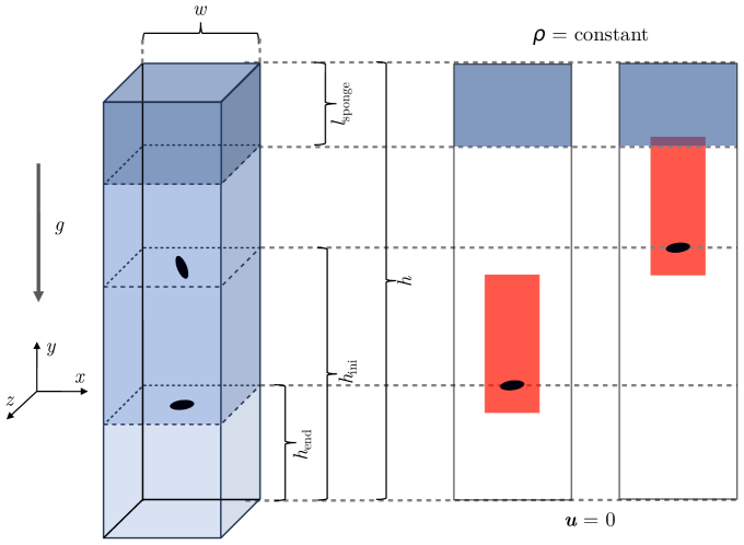
The setup and simulation principles of a numerical free-fall experiment is illustrated in Fig. 1. A particle of arbitrary shape is dropped either from rest or with an initial translational and / or angular velocity, and falls due to gravity in negative $y$-direction. The particle’s translational and rotational vectors are free and are impacted only by gravity and by air pressure and shearing forces. The top boundary, at the maximal $y$-coordinate, implements a constant fluid density, i.e. constant-pressure boundary condition. A sponge zone is additionally defined in the vicinity of the top boundary, to eliminate spurious pressure waves created in the domain by numerical artifacts. In this zone, the fluid viscosity is increased linearly to reach a relaxation time $\tau=1$ on the top boundary. The bottom boundary implements a no-slip condition. The lateral boundaries are periodic.

It should be noted that for the largest simulated particles, with a diameter larger than 1 cm, the distance traversed by a particle until it reaches its terminal velocity is typically three orders of magnitude larger than the particle diameter. Therefore, to avoid the allocation of an impractically large domain, the particle is periodically reinjected at its initial position, as illustrated in Fig. 1. During this copy, the particle population of a full fluid volume directly impacted by the particle motion (indicated in red on the right part of the figure) is copied along with the particle. Also, when the particle drifts close to the lateral boundaries of the domain, a similar fluid volume around the particle is copied and repositioned in the center of the domain. This area is typically elongated above the particle, especially in high-Reynolds flows with a fully developed wake.

It should be pointed out that this iterative reinjection scheme cannot be replaced by a simple periodicity condition between the top and the bottom wall, as such a setup would represent an open system with ever-increasing kinetic energy, under the effect of gravity. Another setup with lateral no-slip wall (instead of a no-slip bottom) would not be acceptable either, because it would represent a motion in a channel with a cross-channel velocity profile that is not representative of particle free-fall in an unbounded fluid.

The simulation setup is caracterized by the domain height $h$ and width $w$, the positions $h_{\mathrm{ini}}$ and $h_{\mathrm{end}}$ for the initial and final position of a particle (before reinjection), the length of the sponge zone $l_{\mathrm{sponge}}$ and the number of lattices, i.e. $N$, spatially discretizes domain width $w$. The kinematic fluid viscosity, $\nu$, the density ratio between the particle and the air, $\kappa$, the volume-equivalent spherical diameter of the particle, $d$, and particle elongation, $el$, and flatness, $fl$, are further provided to complete the specifications of a numerical free-fall experiment. $el=b/a$ is defined as the ratio of the intermediate length $b$ of the particle to its largest length $a$, and $fl=c/b$ is defined as the ratio of the smallest length $c$ of the particle to the intermediate length $b$ [66]. Numerical length parameters are non-dimensionalized with respect to the volume-equivalent spherical diameter $d$, e.g. $w^{*}=w/d$. In all simulations, gravity has a value of 9.81 m²/s. The parameters of all numerical experiments of Section 3 are summarized in Table 2.

3 Results

The numerical free-fall experiment is validated in the following sections at different Reynolds numbers for particles of spherical, spheroidal, and a lapilli-sized volcanic particles. The numerical parameters of the simulations are summarized in Table 2. $N$ is defined as the number of lattice cells used to resolve a particle diameter $d$, where $d$ the longest axis for the ellipsoids. In the case of the arbitrary-shaped volcanic particle, $d$ is the diameter of an equivalent circle of area equal to the cross-sectional are of the broadest particle side. The discrete cell spacing is defined as $\delta x=d/N$. The resolution The time discretization $\delta t$ is fixed by fixing the terminal velocity (analytical, empirical, or experimental prediction) to a value of 0.02 in lattice units.

Physical parameters Numerical parameters Results $d$ [mm] $\kappa$ $\nu$ [$\mathrm{m^{2}/s}$] $el$ $fl$ $w^{*}$ $h^{*}$ $h_{\mathrm{ini}}^{*}$ $h_{\mathrm{end}}^{*}$ $l_{\mathrm{sponge}}^{*}$ $N$ $v_{\mathrm{T}}$ [$\mathrm{m/s}$] $\mathrm{Re}_{T}$ Sphere-1 0.148 996.26 1.51e-5 1.0 1.0 10.0 40.0 35.0 5.0 4.0 400 0.5233 5.12 Sphere-2 0.140 996.26 1.51e-5 1.0 1.0 10.0 40.0 35.0 5.0 4.0 300 0.4848 4.49 Spheroid-1 0.140 996.26 1.51e-5 1.0 0.2 17.1 51.3 46.2 5.1 4.1 550 0.3405 3.15 Spheroid-2 0.140 996.26 1.51e-5 0.2 1.0 29.3 87.9 79.1 8.8 7.0 550 0.3630 3.36

Table 2: Parametrization and summary of results of the virtual free-fall numerical experiments. For simulations with multiple resolution for the same particle, the value of $N$, $v_{\mathrm{T}}$, and $\mathrm{Re}_{T}$ correspond to the simulation with the highest resolution in this table. The right column shows the average terminal velocity $v_{\mathrm{T}}$ reached in the statistically stationary state, as well as the associated Reynolds number $\mathrm{Re}_{T}$.

3.1 Grid convergence

A grid convergence study was conducted at a non-vanishing Reynolds number close to $\mathrm{Re}=5$, using the numerical parameter series ‘Sphere-1’ in Table 2. The study demonstrates a convergence of the drag force on a sphere as a function of grid resolution, and a comparison with the empirical drag predicted in [67] shows a satisfactory convergence of the total force already at a low resolution of 10 grid points (Figure 2). A decomposition into force contributions however shows that pressure force and the shear force, taken individually, are inaccurate at low resolution and start showing signs of grid convergence at a higher resolution of 30 grid points only.

Figure 2: Convergence of the total drag and the relative contributions of pressure and viscous forces as a function of grid resolution.

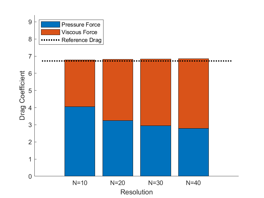
This study shows that sufficient grid convergence is achieved at values of resolution starting at $N=30$. It must be emphasized that proper numerical values of the the pressure and shear components of the force are critically important to model the free-fall behavior, and especially the onset of rotational motion, of particles. While it can be tempting to choose a grid resolution on ground of a convergence study of the drag force alone, it is now clear that this would lead to under-resolved simulations. In conclusion, a resolution of $N=30$ for most of the simulations of finite, low Reynolds number presented below.

3.2 Rotating sphere at low Reynolds number

For the validation of sphere motion in inertial flow at different Reynolds numbers, we compare it to the empirical relationship proposed by Clift & Gauvin [67]. This model presents the standard drag curve throughout the transitional and Newton regimes ($\mathrm{Re}<10^{5}$):

$$C_{D}=(24/\mathrm{Re})(1+0.15\,\mathrm{Re}^{0.687})+0.42/(1+4.25\cdot 10^{4}\,\mathrm{Re}^{-1.16}).$$ (31)

Through time-integration of Newton’s equations of motion, this drag curve translates into a free-fall trajectory of a spherical particle from rest to terminal velocity $v_{\mathrm{T}}$. The equation is solved through an implicit Euler scheme, where the time evolution of the sphere velocity is given by the following Basset-Boussinesque-Oseen equation [68]:

$$\frac{du}{dt}=\frac{1}{\rho+\frac{1}{2}}\left(\kappa g-\frac{9}{2}\frac{v\nu}{r^{2}}-\frac{9}{2}\frac{\nu}{r\pi}\sqrt{\frac{\pi}{\nu}}\int_{0}^{t}\frac{du}{dt^{\prime}}\frac{dt^{\prime}}{\sqrt{t-t^{\prime}}}\right).$$ (32)

A solution for rotational motion was first considered by Basset [69] and later improved by Feuillebois and Lasek [70]. Here, a constant torque $T$ is applied to a sphere initially at rest. The sphere begins to accelerate angularly and ultimately reaches the terminal angular velocity $\omega_{\mathrm{st}}$, given by

$$\omega_{\mathrm{st}}=\frac{T}{m_{\mathrm{sphere}}}\frac{\kappa}{6\nu},$$ (33)

where $m_{\mathrm{sphere}}$ is the mass of the sphere and $\kappa$ is the density ratio between the sphere and the fluid. The time evolution of the angular velocity $\omega$ is described by the relation

$$\frac{d\omega}{dt} =\frac{\rho_{\mathrm{f}}}{I}\left[\frac{T}{\rho_{\mathrm{f}}}-8\pi\nu r^{3}\omega-8\pi\nu r^{3}\left(\frac{r}{3\sqrt{\pi\nu}}\int_{0}^{t}\frac{d\omega}{dt^{\prime}}\frac{dt^{\prime}}{\sqrt{t-t^{\prime}}}\right)\right.$$ (34)

$$\quad\left.+\frac{8}{3}\pi\nu r^{3}\left(\int_{0}^{t}\frac{d\omega}{dt^{\prime}}\exp(\nu(t-t^{\prime})/r^{2})\mathrm{erfc}\sqrt{\nu(t-t^{\prime})/r^{2}}dt^{\prime}\right)\right].$$

For a sphere with homogeneous mass distribution, the moment of inertia $I$ takes the value $I=2/5m_{\mathrm{sphere}}r^{2}$, and the term $\rho_{\mathrm{f}}/I$ in the equation above is given by

$$\frac{\rho_{\mathrm{f}}}{I}=\frac{15}{8}\frac{1}{\kappa r^{5}\pi}.$$ (35)

For the DNS, we considered the equivalent problem of a sphere which, in absence of an external torque, starts rotation under the effect of an ambient linear shear flow. The far-field flow velocity is defined as

$$v_{x}=0,\quad v_{y}=v_{0}+Gy,\quad v_{z}=0,$$ (36)

where the coordinates $x$, $y$, and $z$ represent a fixed reference frame. Here, $G$ is the shear rate of the ambient flow, and we denote the rotation rate of the ambient flow as $\omega_{f}=G/2$. As pointed out for example in [71], the terminal angular velocity of a sphere is equal to the ambient flow rate in a Stokes flow, $\omega_{f}=\omega_{\mathrm{st}}$, while a slip angular velocity is observed at finite Reynolds numbers. We define the Reynolds number in a rotational flow as

$$\mathrm{Re}_{G}=\frac{4Gr^{2}}{\nu},$$ (37)

Leading to the following expression for the torque term in Eq. 34:

$$\frac{T}{\rho_{\mathrm{f}}}=\mathrm{Re}_{G}\frac{9}{16}r\pi\nu^{2}.$$ (38)

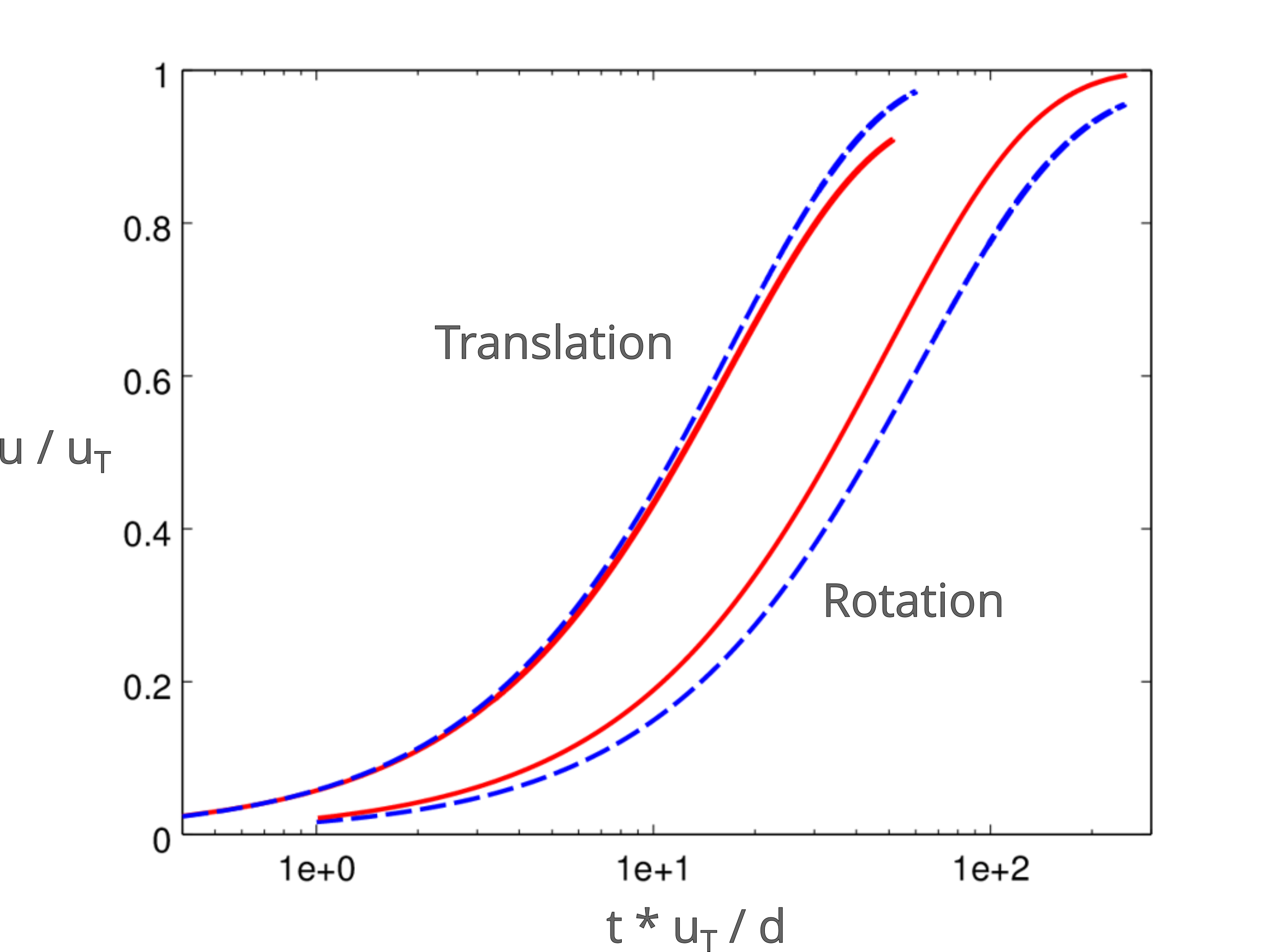
For the DNS, the Reynolds number is fixed to a finite value of $\mathrm{Re}\sim 5$, with simulation parameters as $d=0.140$ mm, $\kappa=1000$, $\nu=1.73e^{-5}\mathrm{m^{2}/s}$, $w^{*}=20$, $h^{*}=30$, $h_{\mathrm{ini}}^{*}=20$, $h_{\mathrm{end}}^{*}=10$, $l_{\mathrm{sponge}}^{*}=3$, and $N=300$. For the rotational motion, a constant torque is applied to the sphere, gravity is disabled, and a no-slip condition without sponge zone is applied on all walls. The numerical results for translational and rotational motion are shown in Figure 3, and compared to the empirical model relations 32 and 34. The simulations show a good match with the analytical curves, although for the translational motion, the terminal velocity is reached slightly faster in the DNS than in the analytical curve. This observation is compatible with the results of a spectral method obtained at a density ratio $\kappa=1.05$ in [72]. As explained further in [72], the discrepancy between analytical and numerical solution is mainly due to the effect of finite Reynolds number. For the rotational motion, the numerical solution matches the analytical one closely, with an cumulative error that builds up due to a long time range spanning over two orders of magnitude.

Figure 3: Free translation (left curve) and free rotation (right curve) in a Stokes flow.

3.3 Terminal velocity of sphere at different Reynolds number

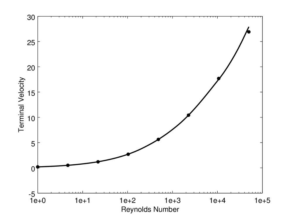
As a next validation case, we measured the terminal velocity $v_{\mathrm{T}}$ of a freely falling sphere. This test is more challenging than a simple numerical evaluation of the sphere drag, as the spheres are moving and rotating and traverse the cells of the fluid grid. The DNS domain boundaries had a fixed extent of $w^{*}=10$ and $h^{*}=30$, and the same resolution of $N=300$. However, depending on the particle Reynolds number $\mathrm{Re}$, $h_{\mathrm{ini}}^{*}=27.0$, $h_{\mathrm{end}}^{*}=3.0$ and $l_{\mathrm{sponge}}^{*}=2.4$ are used when $\mathrm{Re}<30$; $h_{\mathrm{ini}}^{*}=23.0$, $h_{\mathrm{end}}^{*}=3.0$ and $l_{\mathrm{sponge}}^{*}=2.4$ for $20\leq\mathrm{Re}<1000$; and $h_{\mathrm{ini}}^{*}=20.0$, $h_{\mathrm{end}}^{*}=3.0$ and $l_{\mathrm{sponge}}^{*}=2.4$ for $\mathrm{Re}\geq 1000$. The results are summarized in Figure 4 and in Table 3. It can be seen that in a laminar regime, the numerical terminal velocity matches the empirical value with a two to three-digit accuracy, and for higher Reynolds number up to $50,000$, the simulation results remain within a $6\%$ difference from the empirical one.

Figure 4: Free-fall velocity of spheres at various $\mathrm{Re}$, compared to empirical model prediction in Eq. 31.

$\mathrm{Re}^{\mathrm{ref}}$	0.57*	1.36	4.57	5.24	6.34	29.34	129.40	586.36
$d$ [mm]	0.062	0.088	0.140	0.148	0.160	0.315	0.659	1.488
$v_{\mathrm{T}}^{\mathrm{ref}}$ [m/s]	0.138*	0.234	0.493	0.535	0.599	1.408	2.968	5.956
$v_{\mathrm{T}}^{D}$ [m/s]	0.142	0.239	0.485	0.523	0.584	1.358	2.933	6.035
$\Delta v_{\mathrm{T}}$ [%]	2.82	2.09	-1.65	-2.29	-2.57	-3.68	-1.19	1.31
$p^{*}$ [%]	35.80	38.76	42.67	43.10	43.46	48.37	57.50	68.90

Table 3: Evolution of terminal velocities of spheres at different Reynolds number. For reference, a empirical model of [67] is used to approximate the drag force in Eq. 31, and the resulting terminal velocity $v_{\mathrm{T}}^{\mathrm{ref}}$, and the Reynolds number $\mathrm{Re}^{\mathrm{ref}}$. For the low $\mathrm{Re}^{\mathrm{ref}}$ * case, the reference terminal velocity is computed from Stokes’ law: $v_{\mathrm{T}}=(1/18)(\kappa gd^{2}/\nu)$. The terminal velocity obtained from the DNS is shown as $v_{\mathrm{T}}^{D}$, $\Delta v_{\mathrm{T}}=(v_{\mathrm{T}}^{D}-v_{\mathrm{T}}^{\mathrm{ref}})/v_{\mathrm{T}}^{D}$, and $p^{*}$ indicate the contribution of the pressure force to the total drag force at the steady-state. The mass-densities of the sphere and the fluid are $\rho_{\mathrm{p}}=1200$ and $\rho_{\mathrm{f}}=1.2045$ kg/m³ respectively, and the kinematic viscosity of the fluid is $\nu=1.51\times 10^{-5}$ m²/s, representative of the air at 20^oC at the mean sea level.

For validating the time history of settling velocity from the numerical free-fall simulation, a Reynolds of $Re=4.49$ is chosen, with parameters summarized under the label ‘Sphere-2’ in Table 2. Figure 5 compares the obtained numerical and empirical curve of Eq. 31.

Figure 5: Time-evolution of sphere free-fall at finite Reynolds number $Re=4.5$. Comparison between numerical and empirical values.

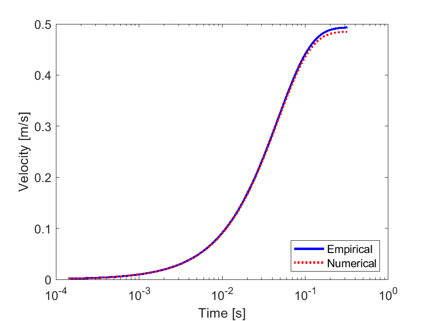
A very close match is obtained for the particle time-evolution, with an expected discrepancy of $2\%-3\%$ regarding the terminal velocity.

3.4 Spheroids

For the investigation of the rotational motion at finite Reynolds number, the next experiments investigates spheroidal particles. The naming adopted is based on the three orthogonal axes $a$, $b$, $c$ of the spheroids, defining shape parameters: $el$ for the elongation $el=b/a$ and $fl$ for the flatness $fl=c/b$. The two investigated cases are of an oblate spheroid (‘Spheroid-1’, $el=1.00$, $fl=0.20$) and a prolate spheroid (‘Spheroid-2’, $el=0.20$, $fl=1.00$), with detailed parameters provided in Table 2. The numerical output is compared to experimental results of settling particle behavior in a settling chamber setup [66].

In this settling chamber experimental setup [17], particles of different shapes with at least one dimension larger than 100 $\mathrm{\mu}$m are tracked three-dimensionally using four high-speed cameras. The vertical distance of free fall in still air is tracked for a vertical distance of $\sim$60 mm. In this experimental setup, it is observed that the heavy ellipsoidal particles undergo transient oscillations to reach their terminal state [17, 66] and that the microplastic fibers exhibit orientation fluctuations depending on their shape and can also have a preferred orientation [16].

Experimental and numerical observations show that spheroidal particles adopt a preferential orientation on their free-fall trajectory, with the side of largest cross-section facing the downward direction. The particle then oscillates around this orientation. To compare the statistics of the free-fall motion, we compared both the average terminal velocity and the highest oscillation frequency, as shown in Table 4. An outstanding match is observed for both quantities, with an error margin within 1% for the terminal velocity and within 2% for the oscillation frequency.

	$el$	$fl$	$v_{\mathrm{T}}^{D}$	$\langle V_{\mathrm{T}}^{E}\rangle$	$\sigma(v_{\mathrm{T}}^{E})$	$f^{D}$	$\langle f^{E}\rangle$	$\sigma(f^{E})$
Spheroid-1 (oblate)	1.00	0.20	0.3405	0.3371	0.0018	40.57	42.02	0.00
Spheroid-2 (prolate)	0.20	1.00	0.3630	0.3519	0.0019	25.57	27.85	2.03

Table 4: Comparison of the numerical and experimental data of non-spherical spheroid particles. The terminal velocity and the frequency of angular oscillations of the particles from the DNS are shown as $v_{\mathrm{T}}^{D}$ and $f^{D}$ respectively. The mean values of the terminal velocity and the frequency of angular oscillations from the experiments are shown as $\langle V_{\mathrm{T}}^{E}\rangle$ and $\langle f^{E}\rangle$, and their standard deviation as $\sigma(v_{\mathrm{T}}^{E})$ and $\sigma(f^{E})$ respectively. All quantities of the velocity and frequency are in units of m/s and Hz respectively.

3.5 General shape – Lapilli

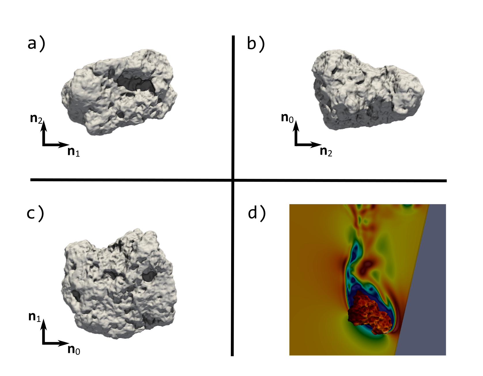
The final validation case considers a specific volcanic particle of the category of Lapilli, which is collected from a field observation of a volcanic eruption. The particle was digitized and converted to a triangularized surface mesh representation, serving both as input for an arbitrary shape in the virtual wind-tunnel simulator, and as a model for 3D-printed particles for reproducible experimental investigations. The numerical parameters of the particle (volume and detailed tensor of inertia) are computed through numerical integration.

The particle has a diameter of the order of 3 cm and reaches a particle Reynolds number above $40,000$ at its terminal velocity. Three orthogonal side views are shown on Figure 6, together with a snapshot of the virtual free-fall simulation. This case is chosen both to illustrate the capability of the numerical solver to represent particles of arbitrary shape and to produce robust results in a turbulent regime.

Figure 6: Depiction of the volcanic particle of the lapilli family used in the numeric simulation. Image a)-c) show three side views and axis of the $({\bm{n}}_{0},{\bm{n}}_{1},{\bm{n}}_{2})$ reference frame that is attached to the particle. Image d) shows a snapshot of the velocity-norm field on a plane that cuts the particle during the virtual free-fall simulation.

This problem is difficult to tackle experimentally, because of the challenges of reproducing free-fall conditions for this Reynolds number in a laboratory setting. A vertical wind-tunnel is inadequate, in part because of turbulence present in the air inlet. Similarly to the observation at lower Reynolds regimes, the selection of a preferential free-fall orientation, as well as oscillatory and spinning motion around this orientation, dictate the statistics, including the average terminal velocity, of the particle. This behavior relies on a realistic representation of ambient conditions aerodynamic conditions.

In this case, the experiment was conducted in exterior conditions involving a free-fall over the order of 30 m, allowing to measure the average terminal velocity, but without access to additional statistics. This emphasizes the need of a numerical simulation tool to complement laboratory experimentation and provide insight into details of the particle motion.

The numerical simulation is conducted with parameters $d=31.80$ mm, $\kappa=959.32$, $\nu=1.87e^{-5}\mathrm{m^{2}/s}$, $el=0.6$, $fl=0.6$, $w^{*}=30$, $h^{*}=13$, $h_{\mathrm{ini}}^{*}=5$, $h_{\mathrm{end}}^{*}=3$, $l_{\mathrm{sponge}}^{*}=3$, and $N=300$. The particle history consists of a succession of states dominated by an oscillation around a preferred orientation or rotation around a preferred axis. For this reason, the time towards convergence of the statistical average for the terminal velocity is very long. Within the interval from 2s to 4.5 s, an average value of $v_{\mathrm{T}}=-23.5m/s$ is obtained, which differs by 8% from the experimental value of $-21.7m/s$.

All in all, this comparison shows a good match between simulation and experiment, while the simulation reveals further insights into possible modes adopted by the particle, and their impact on the obtained terminal velocity.

4 Conclusion

This paper presents a state-of-the-art numerical framework for the study of intricate interactions between particles and air under free-fall conditions. One of the most important features of this framework is its ability to represent particles regardless of their shape complexity, thus ensuring a comprehensive representation of real-world scenarios. Another salient feature is the framework’s ability to simulate extended free-fall distances, a feat made possible by a dynamic memory allocation scheme that accounts for the inherent multi-scale nature of such phenomena. These attributes are further strengthened by careful validation against both analytical and experimental datasets, which have shown the high precision and reliability of the tool.

Our numerical investigations have also revealed several key insights. The first is the necessity to resort to higher resolutions than the one expected at first sight. Indeed, the data show that although integral metrics such as total drag can converge at more moderate resolutions, the precise distribution of force over a particle surface, required to determine the torque, requires much higher resolutions. Furthermore, the relative contribution of pressure and shear terms to the force may still vary at increasing resolution, although the total force remains largely invariant. A second interesting observation is that the proper representation of the rotational dynamics of the particles receives critical importance. The oscillatory motion of particles around a particular side has a pronounced effect, with the selected side, or its statistical patterns, playing a central role in determining the free fall velocity.

In essence, the framework presented in this article serves as a solid foundation and invaluable tool for the in-depth exploration of particle free-fall physics. First applications of this framework and through investigations of particle free-fall physics are presented in [66]. Regarding future work, the next steps involve diving into simulations with dynamic mesh refinement. Although such an endeavor comes with substantial technical difficulties, it promises to further improve the resolution close to the particles. In addition, it paves the way for multi-particle simulations, providing a more comprehensive understanding of the dynamics at play.

Appendix A Regularized LBM: equilibrium and off-equilibrium

The equilibrium and off-equilibrium populations for the regularized lattice Boltzmann method are defined as follows:

$$f^{(0)}_{i}= w_{i}(p/c_{s}^{2}+\rho_{0})\left(1+\frac{\bm{\xi}_{i}\cdot\bm{u}}{c_{s}^{2}}+\frac{1}{2c_{s}^{4}}\mathcal{H}^{(2)}_{i}:\bm{u}\bm{u}\right.$$

$$\quad\quad+\frac{1}{2c_{s}^{6}}\left(\mathcal{H}^{(3)}_{ixxy}u_{x}^{2}u_{y}+\mathcal{H}^{(3)}_{ixxz}u_{x}^{2}u_{z}+\mathcal{H}^{(3)}_{ixyy}u_{x}u_{y}^{2}+\mathcal{H}^{(3)}_{ixzz}u_{x}u_{z}^{2}\right.$$

$$\quad\quad\quad\quad\quad\quad\left.+\mathcal{H}^{(3)}_{iyzz}u_{y}u_{z}^{2}+\mathcal{H}^{(3)}_{iyyz}u_{y}^{2}u_{z}+2\mathcal{H}^{(3)}_{ixyz}u_{x}u_{y}u_{z}\right)$$

$$\quad\quad+\frac{1}{4c_{s}^{8}}\left(\mathcal{H}^{(4)}_{ixxyy}u_{x}^{2}u_{y}^{2}+\mathcal{H}^{(4)}_{ixxzz}u_{x}^{2}u_{z}^{2}+\mathcal{H}^{(4)}_{iyyzz}u_{y}^{2}u_{z}^{2}\right.$$

$$\quad\quad\quad\quad\quad\quad\left.+2\left(\mathcal{H}^{(4)}_{ixyzz}u_{x}u_{y}u_{z}^{2}+\mathcal{H}^{(4)}_{ixyyz}u_{x}u_{y}^{2}u_{z}+\mathcal{H}^{(4)}_{ixxyz}u_{x}^{2}u_{y}u_{z}\right)\right)$$

$$\quad\quad+\frac{1}{4c_{s}^{10}}\left(\mathcal{H}^{(5)}_{ixxyzz}u_{x}^{2}u_{y}u_{z}^{2}+\mathcal{H}^{(5)}_{ixxyyz}u_{x}^{2}u_{y}^{2}u_{z}+\mathcal{H}^{(5)}_{ixyyzz}u_{x}u_{y}^{2}u_{z}^{2}\right)$$

$$\quad\quad\left.+\frac{1}{8c_{s}^{12}}\mathcal{H}^{(6)}_{ixxyyzz}u_{x}^{2}u_{y}^{2}u_{z}^{2}\right),$$ (39)

$$f^{(1)}_{i}= w_{i}\left(\frac{1}{2c_{s}^{4}}\mathcal{H}^{(2)}_{i}:\bm{P}^{(1)}\right.$$

$$\quad\quad+\frac{1}{2c_{s}^{6}}\left(\mathcal{H}^{(3)}_{ixxy}a^{(3)}_{1,xxy}+\mathcal{H}^{(3)}_{ixxz}a^{(3)}_{1,xxz}+\mathcal{H}^{(3)}_{ixyy}a^{(3)}_{1,xyy}+\mathcal{H}^{(3)}_{ixzz}a^{(3)}_{1,xzz}\right.$$

$$\quad\quad\quad\quad\quad\quad\left.+\mathcal{H}^{(3)}_{iyzz}a^{(3)}_{1,yzz}+\mathcal{H}^{(3)}_{iyyz}a^{(3)}_{1,yyz}+2\mathcal{H}^{(3)}_{ixyz}a^{(3)}_{1,xyz}\right)$$

$$\quad\quad+\frac{1}{4c_{s}^{8}}\left(\mathcal{H}^{(4)}_{ixxyy}a^{(4)}_{1,xxyy}+\mathcal{H}^{(4)}_{ixxzz}a^{(4)}_{1,xxzz}+\mathcal{H}^{(4)}_{iyyzz}a^{(4)}_{1,yyzz}\right.$$

$$\quad\quad\quad\quad\quad\quad\left.+2\left(\mathcal{H}^{(4)}_{ixyzz}a^{(4)}_{1,xyzz}+\mathcal{H}^{(4)}_{ixyyz}a^{(4)}_{1,xyyz}+\mathcal{H}^{(4)}_{ixxyz}a^{(4)}_{1,xxyz}\right)\right)$$

$$\quad\quad+\frac{1}{4c_{s}^{10}}\left(\mathcal{H}^{(5)}_{ixxyzz}a^{(5)}_{1,xxyzz}+\mathcal{H}^{(5)}_{ixxyyz}a^{(5)}_{1,xxyyz}+\mathcal{H}^{(5)}_{ixyyzz}a^{(5)}_{1,xyyzz}\right)$$

$$\quad\quad\left.+\frac{1}{8c_{s}^{12}}\mathcal{H}^{(6)}_{ixxyyzz}a^{(6)}_{1,xxyyzz}\right),$$ (40)

$\mathcal{H}_{i}^{(n)}$ is the Hermite polynomial of order $n$. Finally $\bm{a}_{1}^{(n)}$ is given by

$$a^{(n)}_{1,\alpha_{1}...\alpha_{n}} =a^{(n-1)}_{1,\alpha_{1}...\alpha_{n-1}}u_{\alpha_{n}}+\left(u_{\alpha_{1}}...u_{\alpha_{n-2}}P^{(1)}_{\alpha_{n-1}\alpha_{n}}+\hbox{perm}(\alpha_{n})\right)\quad\mathrm{and}$$ (41)

$$\bm{P}^{(1)} =\sum_{i}\bm{\xi}_{i}\bm{\xi}_{i}(f_{i}-f^{(0)}_{i}),$$ (42)

where $\hbox{perm}(\alpha_{n})$ are the cyclic index permutations of indexes from $\alpha_{1}$ to $\alpha_{n-1}$ ($\alpha_{n}$ is never permuted).

References

- Pruppacher and Klett [2010] H. R. Pruppacher, J. D. Klett, Microphysics of Clouds and Precipitation, second ed., Springer, Dordrecht, 2010. doi:10.1007/978-0-306-48100-0.
- Rossi et al. [2021] E. Rossi, G. Bagheri, F. Beckett, C. Bonadonna, The fate of volcanic ash: premature or delayed sedimentation?, Nature Communications 12 (2021) 1303. doi:10.1038/s41467-021-21568-8.
- van der Does et al. [2018] M. van der Does, P. Knippertz, P. Zschenderlein, R. G. Harrison, J.-B. W. Stuut, The mysterious long-range transport of giant mineral dust particles, Science Advances 4 (2018) eaau2768. doi:10.1126/sciadv.aau2768.
- van Hout and Katz [2004] R. van Hout, J. Katz, A method for measuring the density of irregularly shaped biological aerosols such as pollens, Journal of Aerosol Science 35 (2004) 1369–1384. doi:10.1016/j.jaerosci.2004.05.008.
- Heymsfield [1973] A. J. Heymsfield, Laboratory and field observations of the growth of columnar and plate crystals from frozen droplets, Journal of the Atmospheric Sciences 30 (1973) 1650–1656. doi:10.1175/1520-0469(1973)030<1650:LAFOOT>2.0.CO;2.
- Trudnowska et al. [2021] E. Trudnowska, L. Lacour, M. Ardyna, A. Rogge, J. O. Irisson, A. M. Waite, M. Babin, L. Stemmann, Marine snow morphology illuminates the evolution of phytoplankton blooms and determines their subsequent vertical export, Nature communications 12 (2021) 2816. doi:10.1038/s41467-021-22994-4.
- Xiao et al. [2023] S. Xiao, Y. Cui, J. Brahney, N. M. Mahowald, Q. Li, Long-distance atmospheric transport of microplastic fibres influenced by their shapes, Nature Geoscience 16 (2023) 863–870. doi:10.1038/s41561-023-01264-6.
- Willmarth et al. [1964] W. W. Willmarth, N. E. Hawk, R. L. Harvey, Steady and unsteady motions and wakes of freely falling disks, Physics of Fluids 7 (1964) 197–208. doi:10.1063/1.1711133.
- Khayat and Cox [1989] R. Khayat, R. Cox, Inertia effects on the motion of long slender bodies, Journal of Fluid Mechanics 209 (1989) 435–462. doi:10.1017/S0022112089003174.
- Newsom and Bruce [1994] R. K. Newsom, C. W. Bruce, The dynamics of fibrous aerosols in a quiescent atmosphere, Physics of Fluids 6 (1994) 521–530. doi:10.1063/1.868347.
- Bagheri and Bonadonna [2016] G. Bagheri, C. Bonadonna, On the drag of freely falling non-spherical particles, Powder Technology 301 (2016) 526–544. doi:10.1016/j.powtec.2016.06.015.
- Gustavsson et al. [2019] K. Gustavsson, M. Z. Sheikh, D. Lopez, A. Naso, A. Pumir, B. Mehlig, Effect of fluid inertia on the orientation of a small prolate spheroid settling in turbulence, New Journal of Physics 21 (2019) 083008. doi:10.1088/1367-2630/ab3062.
- Ouchene [2020] R. Ouchene, Numerical simulation and modeling of the hydrodynamic forces and torque acting on individual oblate spheroids, Physics of Fluids 32 (2020) 073303–. doi:10.1063/5.0011618.
- Alipour et al. [2021] M. Alipour, M. De Paoli, S. Ghaemi, A. Soldati, Long non-axisymmetric fibres in turbulent channel flow, Journal of Fluid Mechanics 916 (2021) A3. doi:10.1017/jfm.2021.185.
- Tinklenberg et al. [2023] A. Tinklenberg, M. Guala, F. Coletti, Thin disks falling in air, Journal of Fluid Mechanics 962 (2023) A3. doi:10.1017/jfm.2023.209.
- Tatsii et al. [2023] D. Tatsii, S. Bucci, T. Bhowmick, J. Guettler, L. Bakels, G. Bagheri, A. Stohl, Shape matters: long-range transport of microplastic fibers in the atmosphere, Environmental Science & Technology 58 (2023) 671–682. doi:10.1021/acs.est.3c08209.
- Bhowmick et al. [2024] T. Bhowmick, J. Seesing, K. Gustavsson, J. Guettler, Y. Wang, A. Pumir, B. Mehlig, G. Bagheri, Inertia Induces Strong Orientation Fluctuations of Nonspherical Atmospheric Particles, Physical Review Letters 132 (2024) 034101. doi:10.1103/PhysRevLett.132.034101.
- Hou et al. [2012] G. Hou, J. Wang, A. Layton, Numerical methods for fluid-structure interaction — a review, Communications in Computational Physics 12 (2012) 337–377. doi:10.4208/cicp.291210.290411s.
- Mittal and Iaccarino [2005] R. Mittal, G. Iaccarino, Immersed boundary methods, Annual Review of Fluid Mechanics 37 (2005) 239–261. doi:10.1146/annurev.fluid.37.061903.175743.
- Tenneti and Subramaniam [2014] S. Tenneti, S. Subramaniam, Particle-resolved direct numerical simulation for gas-solid flow model development, Annual Review of Fluid Mechanics 46 (2014) 199–230. doi:10.1146/annurev-fluid-010313-141344.
- Griffith and Patankar [2020] B. E. Griffith, N. A. Patankar, Immersed methods for fluid–structure interaction, Annual Review of Fluid Mechanics 52 (2020) 421–448. doi:10.1146/annurev-fluid-010719-060228.
- Ma et al. [2022] H. Ma, L. Zhou, Z. Liu, M. Chen, X. Xia, Y. Zhao, A review of recent development for the cfd-dem investigations of non-spherical particles, Powder Technology 412 (2022) 117972. doi:10.1016/j.powtec.2022.117972.
- Rettinger and Rüde [2018] C. Rettinger, U. Rüde, A coupled lattice boltzmann method and discrete element method for discrete particle simulations of particulate flows, Computers & Fluids 172 (2018) 706–719. doi:10.1016/j.compfluid.2018.01.023.
- Rettinger and Rüde [2022] C. Rettinger, U. Rüde, An efficient four-way coupled lattice boltzmann – discrete element method for fully resolved simulations of particle-laden flows, Journal of Computational Physics 453 (2022) 110942. doi:10.1016/j.jcp.2022.110942.
- Thornton and Marion [2004] S. Thornton, J. Marion, Classical Dynamics of Particles and Systems, Brooks/Cole, 2004.
- Greenwood [1988] D. T. Greenwood, Principles of dynamics, Prentice-Hall Englewood Cliffs, NJ, 1988.
- Parsa et al. [2012] S. Parsa, E. Calzavarini, F. Toschi, G. A. Voth, Rotation rate of rods in turbulent fluid flow, Physical Review Letters 109 (2012) 134501. doi:10.1103/PhysRevLett.109.134501.
- Auguste et al. [2013] F. Auguste, J. Magnaudet, D. Fabre, Falling styles of disks, Journal of Fluid Mechanics 719 (2013) 388–405. doi:10.1017/jfm.2012.602.
- Voth and Soldati [2017] G. A. Voth, A. Soldati, Anisotropic particles in turbulence, Annual Review of Fluid Mechanics 49 (2017) 249–276. doi:10.1146/annurev-fluid-010816-060135.
- Sheikh et al. [2020] M. Z. Sheikh, K. Gustavsson, E. Leveque, B. Mehlig, A. Pumir, A. Naso, Importance of fluid inertia for the orientation of spheroids settling in turbulent flow, Journal of Fluid Mechanics 886 (2020) A9. doi:10.1175/JAS-D-21-0305.1.
- AlMomani et al. [2008] T. AlMomani, H. Udaykumar, J. Marshall, K. Chandran, Micro-scale dynamic simulation of erythrocyte–platelet interaction in blood flow, Annals of biomedical engineering 36 (2008) 905–920. doi:10.1007/s10439-008-9478-z.
- Freund [2014] J. B. Freund, Numerical simulation of flowing blood cells, Annual Review of Fluid Mechanics 46 (2014) 67–95. doi:10.1146/annurev-fluid-010313-141349.
- Ye et al. [2016] T. Ye, N. Phan-Thien, C. T. Lim, Particle-based simulations of red blood cells—a review, Journal of Biomechanics 49 (2016) 2255–2266. doi:10.1016/j.jbiomech.2015.11.050.
- Latt et al. [2021] J. Latt, O. Malaspinas, D. Kontaxakis, A. Parmigiani, D. Lagrava, F. Brogi, M. B. Belgacem, Y. Thorimbert, S. Leclaire, S. Li, et al., Palabos: parallel lattice boltzmann solver, Computers & Mathematics with Applications 81 (2021) 334–350. doi:10.1016/j.camwa.2020.03.022.
- Coreixas [2018] C. G. Coreixas, High-order extension of the recursive regularized lattice Boltzmann method, Ph.D. thesis, Institut National Polytechnique de Toulouse-INPT, 2018.
- Coreixas et al. [2019] C. Coreixas, B. Chopard, J. Latt, Comprehensive comparison of collision models in the lattice boltzmann framework: Theoretical investigations, Physical Review E 100 (2019) 033305. doi:10.1103/PhysRevE.100.033305.
- Hu et al. [1992] H. H. Hu, D. D. Joseph, M. J. Crochet, Direct simulation of fluid particle motions, Theoretical and Computational Fluid Dynamics 3 (1992) 285–306. doi:10.1007/BF00717645.
- Feng et al. [1994a] J. Feng, H. H. Hu, D. D. Joseph, Direct simulation of initial value problems for the motion of solid bodies in a newtonian fluid part 1. sedimentation, Journal of Fluid Mechanics 261 (1994a) 95–134. doi:10.1017/S0022112094000285.
- Feng et al. [1994b] J. Feng, H. H. Hu, D. D. Joseph, Direct simulation of initial value problems for the motion of solid bodies in a newtonian fluid. part 2. couette and poiseuille flows, Journal of Fluid Mechanics 277 (1994b) 271–301. doi:doi:10.1017/S0022112094002764.
- Ladd [1994a] A. J. C. Ladd, Numerical simulations of particulate suspensions via a discretized boltzmann equation. part 1. theoretical foundation, Journal of Fluid Mechanics 271 (1994a) 285–309. doi:10.1017/S0022112094001771.
- Ladd [1994b] A. J. C. Ladd, Numerical simulations of particulate suspensions via a discretized boltzmann equation. part 2. numerical results, Journal of Fluid Mechanics 271 (1994b) 311–339. doi:10.1017/S0022112094001783.
- Aidun and Lu [1995] C. Aidun, Y. Lu, Lattice boltzmann simulation of solid particles suspended in fluid, Journal of Statistical Physics 81 (1995) 49–61. doi:10.1007/BF02179967.
- Johnson and Tezduyar [1995] A. A. Johnson, T. E. Tezduyar, Simulation of multiple spheres falling in a liquid-filled tube, Computer Methods in Applied Mechanics and Engineering 134 (1995) 351–373. doi:10.1016/0045-7825(95)00988-4.
- Glowinski et al. [1999] R. Glowinski, T. W. Pan, T. I. Hesla, D. D. Joseph, A distributed lagrange multiplier/fictitious domain method for particulate flows, International Journal of Multiphase Flow 25 (1999) 755 – 794. doi:10.1016/S0301-9322(98)00048-2.
- Verberg and Ladd [2000] R. Verberg, A. J. C. Ladd, Lattice-boltzmann model with sub-grid-scale boundary conditions, Phys. Rev. Lett. 84 (2000) 2148–2151. doi:10.1103/PhysRevLett.84.2148.
- Verberg and Ladd [2001] R. Verberg, A. J. C. Ladd, Accuracy and stability of a lattice-boltzmann model with subgrid scale boundary conditions, Phys. Rev. E 65 (2001) 016701. doi:10.1103/PhysRevE.65.016701.
- Takagi et al. [2003] S. Takagi, H. N. Oguz, Z. Zhang, A. Prosperetti, Physalis: a new method for particle simulation: Part ii: two-dimensional navier?stokes flow around cylinders, Journal of Computational Physics 187 (2003) 371–390. doi:10.1016/S0021-9991(03)00077-9.
- Zhang and Prosperetti [2003] Z. Zhang, A. Prosperetti, A method for particle simulation, Journal of Applied Mechanics 70 (2003) 64–74. doi:10.1115/1.1530636.
- Feng and Michaelides [2004] Z.-G. Feng, E. E. Michaelides, The immersed boundary-lattice boltzmann method for solving fluid-particles interaction problems, J. Comput. Phys. 195 (2004) 602–628. doi:10.1016/j.jcp.2003.10.013.
- Li et al. [2004] H. Li, H. Fang, Z. Lin, S. Xu, S. Chen, Lattice boltzmann simulation on particle suspensions in a two-dimensional symmetric stenotic artery, Phys. Rev. E 69 (2004) 031919. doi:10.1103/PhysRevE.69.031919.
- Strack and Cook [2007] O. E. Strack, B. K. Cook, Three-dimensional immersed boundary conditions for moving solids in the lattice-boltzmann method, International Journal for Numerical Methods in Fluids 55 (2007) 103–125. doi:10.1002/fld.1437.
- Hölzer and Sommerfeld [2009] A. Hölzer, M. Sommerfeld, Lattice boltzmann simulations to determine drag, lift and torque acting on non-spherical particles, Computers & Fluids 38 (2009) 572 – 589. doi:10.1016/j.compfluid.2008.06.001.
- Guo et al. [2011] X. Guo, J. Lin, D. Nie, New formula for drag coefficient of cylindrical particles, Particuology 9 (2011) 114 – 120. doi:10.1016/j.partic.2010.07.027.
- Wang et al. [2013] L. Wang, Z. Guo, B. Shi, C. Zheng, Evaluation of three lattice boltzmann models for particulate flows, Communications in Computational Physics 13 (2013) 1151–1172. doi:10.4208/cicp.160911.200412a.
- Ginzburg et al. [2023] I. Ginzburg, G. Silva, F. Marson, B. Chopard, J. Latt, Unified directional parabolic-accurate lattice boltzmann boundary schemes for grid-rotated narrow gaps and curved walls in creeping and inertial fluid flows, Physical Review E 107 (2023) 025303. doi:10.1103/PhysRevE.107.025303.
- Thorimbert et al. [2018] Y. Thorimbert, F. Marson, A. Parmigiani, B. Chopard, J. Latt, Lattice boltzmann simulation of dense rigid spherical particle suspensions using immersed boundary method, Computers & Fluids 166 (2018) 286–294. doi:10.1016/j.compfluid.2018.02.013.
- Bagheri et al. [2013] G. H. Bagheri, C. Bonadonna, I. Manzella, P. Pontelandolfo, P. Haas, Dedicated vertical wind tunnel for the study of sedimentation of non-spherical particles, Review of Scientific Instruments 84 (2013) 054501. doi:10.1063/1.4805019.
- Shan et al. [2006] X. Shan, X. F. Yuan, H. Chen, Kinetic theory representation of hydrodynamics: a way beyond the Navier-Stokes equation, J. Fluid Mech. 550 (2006) 413–441. doi:10.1017/S0022112005008153.
- Malaspinas [2015] O. Malaspinas, Increasing stability and accuracy of the lattice Boltzmann scheme: recursivity and regularization, 2015. doi:10.48550/arXiv.1505.06900.
- Bhatnagar et al. [1954] P. L. Bhatnagar, E. P. Gross, M. Krook, A Model for Collision Processes in Gases. I. Small Amplitude Processes in Charged and Neutral One-Component Systems, Phys. Rev. 94 (1954) 511–525. doi:10.1103/PhysRev.94.511.
- Chapman and Cowling [1960] S. Chapman, T. G. Cowling, The mathematical theory of nonuniform gases, Cambridge University Press, Cambridge, 1960.
- Peskin [1972] C. S. Peskin, Flow patterns around heart valves: a numerical method, Journal of Computational Physics 10 (1972) 252 – 271. doi:10.1016/0021-9991(72)90065-4.
- Fadlun et al. [2000] E. A. Fadlun, R. Verzicco, P. Orlandi, J. Mohd-Yusof, Combined immersed-boundary finite-difference methods for three-dimensional complex flow simulations, Journal of Computational Physics 161 (2000) 35–60. doi:10.1006/jcph.2000.6484.
- Wang et al. [2008] Z. Wang, J. Fan, K. Luo, Combined multi-direct forcing and immersed boundary method for simulating flows with moving particles, Int. J of Multiphase Flow 34 (2008) 283–302. doi:10.1016/j.ijmultiphaseflow.2007.10.004.
- Ota et al. [2012] K. Ota, K. Suzuki, T. Inamuro, Lift generation by a two-dimensional symmetric flapping wing: immersed boundary-lattice Boltzmann simulations, Fluid Dyn. Res. 44 (2012) 045504. doi:10.1088/0169-5983/44/4/045504.
- Bhowmick et al. [2024] T. Bhowmick, Y. Wang, J. Latt, G. Bagheri, Twist, turn and encounter: the trajectories of small atmospheric particles unravelled, 2024. doi:10.48550/arXiv.2408.11487.
- Clift and Gauvin [1971] R. Clift, W. H. Gauvin, Motion of entrained particles in gas streams, The Canadian Journal of Chemical Engineering 49 (1971) 439–448. doi:10.1002/cjce.5450490403.
- Zhu and Fan [1998] C. Zhu, L.-S. Fan, Chapter 18. multiphase flow: Gas/solid, in: R. W. Johnson (Ed.), The Handbook of Fluid Dynamics, Springer, 1998.
- Basset [1888] A. B. Basset, A treatise on hydrodynamics with numerous examples, Volume II., Deighton, Bell and co., Cambridge, 1888.
- Feuillebois and Lasek [1978] F. Feuillebois, A. Lasek, On the rotational historic term in non-stationary stokes flow, The Quarterly Journal of Mechanics and Applied Mathematics 31 (1978) 435–443. doi:10.1093/qjmam/31.4.435.
- Lin et al. [1970] C.-J. Lin, J. H. Peery, W. R. Schowalter, Simple shear flow round a rigid sphere: inertial effects and suspension rheology, Journal of Fluid Mechanics 44 (1970) 1–17. doi:10.1017/S0022112070001659.
- Bagchi and Balachandar [2002] P. Bagchi, S. Balachandar, Effect of free rotation on the motion of a solid sphere in linear shear flow at moderate re, Physics of Fluids 14 (2002) 2719–2737. doi:10.1063/1.1487378.