Finding Convincing Views to Endorse a Claim

Abstract.

Recent studies investigated the challenge of assessing the strength of a given claim extracted from a dataset, particularly the claim’s potential of being misleading and cherry-picked. We focus on claims that compare answers to an aggregate query posed on a view that selects tuples. The strength of a claim amounts to the question of how likely it is that the view is carefully chosen to support the claim, whereas less careful choices would lead to contradictory claims. We embark on the study of the reverse task that offers a complementary angle in the critical assessment of data-based claims: given a claim, find useful supporting views. The goal of this task is twofold. On the one hand, we aim to assist users in finding significant evidence of phenomena of interest. On the other hand, we wish to provide them with machinery to criticize or counter given claims by extracting evidence of opposing statements.

To be effective, the supporting sub-population should be significant and defined by a “natural” view. We discuss several measures of naturalness and propose ways of extracting the best views under each measure (and combinations thereof). The main challenge is the computational cost, as naïve search is infeasible. We devise anytime algorithms that deploy two main steps: (1) a preliminary construction of a ranked list of attribute combinations that are assessed using fast-to-compute features, and (2) an efficient search for the actual views based on each attribute combination. We present a thorough experimental study that shows the effectiveness of our algorithms in terms of quality and execution cost. We also present a user study to assess the usefulness of the naturalness measures.

1. Introduction

Data collected rigorously can be used to identify important phenomena in an arguably objective manner. Hence, evidence from data is often used to qualify stated claims. Yet, for this reason, data-based arguments involve considerable risks. Cherrypicking, for instance, refers to basing the claim on a query with specific components that may seem natural, but are nevertheless crucial for supporting the claim rather than its opposite. The risk also goes in the other direction: basing a claim on the general population may give the false impression that the claim holds in important subpopulations (an extreme manifestation of this falsehood is the Simpson’s Paradox). Past work proposed ways of assessing whether a given claim, commonly phrased as an aggregate query over a database, is cherry-picked (Lin et al., 2021; Asudeh et al., 2020, 2021; Lin et al., 2022). This can be seen as a branch in the more general area of computational fact-checking (Guo et al., 2022; Karagiannis et al., 2020; Zhou and Zafarani, 2020; Farinha and Carvalho, 2018; Hassan et al., 2017b; Wu et al., 2014, 2017). Relevant techniques involve machine learning (Lin et al., 2021), query perturbation (Wu et al., 2014, 2017; Asudeh et al., 2020, 2021), and Natural Language Processing (NLP) (Farinha and Carvalho, 2018; Hassan et al., 2017b).

In this work, we study this task in the reverse direction: given a claim that is false in the database, we aim to find natural views where the claim holds. We refer to this problem as claim endorsement. The objective is to enrich people’s machinery with a complementary tool for the critical assessment of claims. In particular, effective claim endorsement can help users better understand the mechanism of cherry-picking and its involved risks. It can also allow users to look for queries that weaken or invalidate a stated claim; for example, a user can look for alternative phrasings that seem just as natural, yet support the opposite claim on the same database. Such an exercise can further help users assess how amenable a particular dataset is to support contradictory claims, and how suspicious we should be, in general, regarding allegations drawn from this dataset. Such abilities may be useful in many domains. For example, they may be used to closely inspect the claims of political candidates, or explore the extent of social issues. They could also be applied in journalism, academic research, and various fields where critical analysis of data-driven claims is crucial.

Example 1.1.

Consider the Stack Overflow Developers Survey dataset that includes information about Hi-Tech workers such as backgrounds, demographics, and annual salaries. In this dataset, the average salary of people with a master’s degree is lower than that of people with only a bachelor’s degree. Alex, a social scientist, aims to challenge this observation. She may do so to understand the potential of cherry-picking by a malicious party, to explore the extent of the phenomenon, or to find out whether the dataset can still support the master’s degree. Hence, she seeks support for the claim that individuals with a master’s degree earn more, on average, than those with a bachelor’s degree. She finds that the claim holds for people in the field of Data Science and Machine Learning (Subpopulation I). It also holds for people in Germany. In addition, she finds less compelling subpopulations, like people who use Zoom for office communication (Subpopulation II), and people who do not know the size of their organization. ∎

The example illustrates that to be effective, the views that endorse the claim should be as significant and “natural” to support for the claim. As the notion of “natural” subpopulations is subjective, we incorporate various measures of naturalness. These measures are drawn from different fields such as information theory, NLP, and statistics. For instance, drawing from past proposals (Wu and Madden, 2013; Tao et al., 2022), one simple measure evaluates the subpopulation’s size, with a larger size indicating broader applicability of the claim. Another measure assesses the claim’s strength within a subpopulation, determined through tests of statistical significance (Wasserman, 2004). Additionally, naturalness can be inferred based on the linguistic relationship between the target attribute and the predicate that defines the view, using language models such as sentence transformers (Reimers and Gurevych, 2019) (as we adopt in our implementation). Our proposed framework is designed to identify and extract the highest-scoring views under each measure, as well as combinations of measures, for a given user claim.

Example 1.2.

We continue Example 1.1, and focus on Subpopulations I and II.The definition of Subpopulation II is, arguably, more artificial and arbitrary, hence less convincing; Subpopulation I appears more natural and supportive of the claim. This intuition is captured by various measures of naturalness. First, Subpopulation I is larger (1446 individuals vs. 743). Second, the criterion of “office synchronous communication tool” is quite unexpected due to lack of connection to salaries and/or academic degrees; we aim to capture this difference through measures from statistics and NLP. Third, within Subpopulation I, master’s people earn considerably more than bachelor’s (average of $183K vs. $144K), whereas the advantage in Subpopulation II is modest ($117K compared to $112K). These considerations are indeed reflected by lower scores for Subpopulation IIaccording to the naturalness measures that we consider in this paper. See Section 5.2 for additional examples. ∎

In more formal terms, we define (in Section 2) the problem of claim endorsement as follows. We are given a SQL query $Q$ with grouping and aggregation (e.g., Average) over a database (relation) $D$, along with a claim stating that the aggregate value of one group is higher than that of another group. We seek useful refinements that restrict $Q$ by adding predicates $p$ to the selection condition of $Q$, so that the claim holds true in the refined query. The goal is to compute the top-$k$ refinements according to a function $\nu$ that quantifies the naturalness of each refinement (in the context of $Q$ and $D$). As aforesaid, we discuss a collection of basic measures of naturalness that cover different aspects of what “natural” can be. Hence, a system can solve multiple instances of the problem with different measures (as we present in our implementation).

The goal in claim endorsement is to find a natural sub-population supporting the claim, which will convince a critical listener of the claim’s truth. In effect, we do so by refining the query representing the claim with the condition of the sub-population. However, our focus is on the original claim, and finding the views that support it.

The main technical challenge that we address (Section 4) is the high computational cost of claim endorsement: refinements can be made out of many attributes, attribute combinations, and value assignments; moreover, each candidate refinement may require costly computation to verify its correctness and measure its naturalness. Efficiency is critical when claim endorsement is used within data exploration, where the user may interactively react to the results of some claims to formulate new ones; response times of days or even hours render the tool ineffective. In particular, listing all possible refinements before ranking is too costly. Similar challenges have been encountered in the search for drill-down and roll-up operators to find the most interesting data parts for exploration (Agarwal et al., 1996; Sathe and Sarawagi, 2001; Joglekar et al., 2017; Youngmann et al., 2022), the discovery of intriguing data visualizations and explanations (Vartak et al., 2015; Deutch et al., 2022), and the explanation of outliers in aggregate queries (Wu and Madden, 2013; Li et al., 2021). However, the algorithms in that body of work cannot be applied in our setting where the requirement is to satisfy the claim and, at the same time, achieve high scores of naturalness measures, as they satisfy neither requirement (see Section 6).

Instead of materializing all possible candidates, we devise a framework for anytime algorithms that target the incremental generation of high-quality refinements from the very beginning. We instantiate the framework on the aforementioned measures of naturalness. More technically, the algorithms enumerate refinements in a ranked fashion, where the ranking function is, intuitively, well correlated with the naturalness measure, yet efficient to handle. Our framework deploys two main steps: (1) produce a ranked list of attribute combinations according to an easy-to-compute scoring function. (2) for each attribute combination $C$ (in ranked order), compute all value assignments for the corresponding refinements. For each step, we develop several solutions and optimizations that we evaluate in the experiments.

We present a thorough experimental study (Section 5) on three datasets: American Community Survey, Stack Overflow, and a flight-delays dataset. These datasets differ in the number of attributes (from tens to hundreds) and number of tuples (from tens of thousands to millions). We show that our anytime algorithms typically achieve 95% of the quality of the true top-$k$ refinements faster than existing baselines by one-to-two orders of magnitudes. We also present case studies on the three datasets, similarly to Example 1.1.

Additionally, we report a user study that we have conducted to assess how well our proposed naturalness measures align with intuitive concepts, and to compare them to existing solutions. Our study indicates that these measures effectively capture aspects of intuitive naturalness and, furthermore, that they align better with intuition than measures adapted from previous work (e.g., (Salimi et al., 2018a)).

In summary, our contributions are as follows: (a) We introduce the claim-endorsement problem. (b) We introduced the concept of naturalness measures for claim endorsement, and proposed several concrete measures, adjusted to the context of this problem. (c) We devise an anytime framework for claim endorsement. (d) We instantiate the framework with algorithms for the proposed measures of naturalness. (e) We present an experimental study that shows the effectiveness of our solutions and analyzes several case studies, and a user study to assess the effectiveness of the naturalness measures.

2. Formal Framework

In this section, we describe our formal model and define the problem of claim endorsement. We begin with preliminary definitions.

Table 1. Records from ACS (Ding et al., 2021) used as a running example.

ID	Sex	Occupation	EducationLevel	QoB	Income (K)
1	F	CS&Math	Bachelor’s degree	1	72
2	F	CS&Math	Master’s degree	3	95
3	F	Education	Master’s degree	2	43
4	F	Sales	High School Diploma	1	35
5	F	Sales	Bachelor’s degree	4	100
6	M	CS&Math	Bachelor’s degree	4	80
7	M	CS&Math	Master’s degree	3	90
8	M	Education	Master’s degree	2	62
9	M	Sales	Bachelor’s degree	1	70
10	M	Sales	High School Diploma	3	65

2.1. Databases and Queries

We consider an input database $D$ that consists of a single relation with the relation name $R$ and the attribute set $\mathord{\mathrm{Att}(D)}{=}\{A_{1},{\ldots},A_{q}\}$. Note that this relation can be the result of a query that joins multiple source relations that are outside of the model (as is indeed the case in our experiments with the Flights dataset; see Section 5). We denote by $|D|$ the number of tuples of $D$. By $D[A_{i_{1}},{\dots},A_{i_{\ell}}]$ we denote the (set-semantics) projection of $D$ to the attributes $A_{i_{1}},{\dots},A_{i_{\ell}}$. By a slight abuse of notation, for a single attribute $A_{i}$ we may view $D[A_{i}]$ as the set of values rather than single-value tuples.

We assume an aggregate SQL query $Q$ of the following form.

(1) SELECT $$A_{gb} \alpha(A_{agg}) \phi A_{gb}$$, FROM D WHERE GROUP BY

where $A_{gb}\in\mathord{\mathrm{Att}(D)}$ is the group-by attribute, $A_{agg}\in\mathord{\mathrm{Att}(D)}$ is the aggregate attribute, and $\alpha$ is an aggregate function among $\mathsf{Count}$, $\mathsf{Sum}$, $\mathsf{Average}$, $\mathsf{Median}$, $\mathsf{Min}$ and $\mathsf{Max}$. We will refer to a query of this form as a group-aggregate query. The result of $Q$ on $D$, denoted $Q(D)$, is a set of tuples of the form $(g,v)$, where $g\in D[A_{gb}]$ and

$$v=\alpha(\{t.A_{agg}\mid t\in D\land\phi(t)\land t.A_{gb}=g\})\,.$$

Example 2.1.

Consider the sample of the ACS dataset (Ding et al., 2021) shown in Table 1. An analyst may be interested in justifying a Master’s degree, so they will first issue the query $Q$:

 SELECT EducationLevel, Average(Income)
FROM D
GROUP BY EducationLevel;  In $Q(D)$, we find that the average income for people with a Master’s degree ($72.5K) is lower than that of Bachelor’s degree ($80.5K).∎

2.2. Claims and Refinements

Similarly to previous work in the context of query result explanations (Li et al., 2021; Ma et al., 2023; Roy and Suciu, 2014a; Tao et al., 2022), we study the case where the analyst restricts attention to the relationship between two groups of interest, $g_{1}$ and $g_{2}$, in the result $Q(D)$. For these, the analyst may be interested in endorsing a specific claim. We define it formally as follows:

Definition 2.2 (Claim).

Consider two tuples $(g_{1},v_{1})$ and $(g_{2},v_{2})$ in $Q(D)$. We refer to the tuple $\kappa=(g_{1},g_{2},>)$ as a claim. A group-aggregate query $Q^{\prime}$ endorses $\kappa$ (on $D$), denoted $Q^{\prime}(D)\models\kappa$, if there are numbers $v_{1}^{\prime}$ and $v_{2}^{\prime}$ such that $(g_{1},v_{1}^{\prime})\in Q^{\prime}(D)$ and $(g_{2},v_{2}^{\prime})\in Q^{\prime}(D)$ and $v_{1}^{\prime}>v_{2}^{\prime}$.

We consider the situation where $Q$ violates $(g_{1},g_{2},>)$, and seek a refinement $Q^{\prime}$ that satisfies it. We focus on refinements that add predicates to the WHERE clause (as done previously, e.g., (Lin et al., 2021)).

Example 2.3.

Following Example 2.1, the analyst wishes to compare the average income for different degree holders, with the initial assumption that a higher degree implies a higher salary. Yet, she finds that the average income for people with a Master’s degree ($72.5K) is actually lower than that of people with a Bachelor’s degree ($80.5K). In our formalism, the analyst is interested in the relationship between $g_{1}=\mathsf{Master^{\prime}s}$ and $g_{2}=\mathsf{Bachelor^{\prime}s}$ and their corresponding values in $Q(D)$, namely $v_{1}=72.5$ and $v_{2}=80.5$. Hence, the claim $(\mathsf{Master^{\prime}s},\mathsf{Bachelor^{\prime}s},>)$ is violated by $Q$. ∎

In this paper, we study the problem of searching for query refinements. To that end, we assume a space $\mathcal{P}$ of predicates that can be used to refine the query $Q$. We consider equality predicates of the form $A{=}v$, where $v{\in}D[A]$, and conjunctions of up to $m$ such predicates, where $m$ is a parameter. This practice has been commonly used in prior work about query answer explanations (Lin et al., 2021; Roy and Suciu, 2014b; Wu and Madden, 2013; El Gebaly et al., 2014; Miao et al., 2019). More formally, we are given a set of split attributes from $\mathord{\mathrm{Att}(D)}$ that does not include $A_{gb}$ and $A_{agg}$, and we denote this set by $\mathrm{SAtt}(D)$. Then $\mathcal{P}$ consists of all predicates of the form $A_{1}=v_{1}\land\dots\land A_{\ell}=v_{\ell}$ such that $\ell\leq m$, $A_{i}\in\mathrm{SAtt}(D)$ and $v_{i}\in D[A_{i}]$ for all $i=1,\dots,\ell$. An atom or atomic predicate is a predicate of the form $A_{i}=v_{i}$. Given a predicate $p$ of this form, denote by $Att(p)=(A_{1},\dots,A_{\ell})$ the set of attributes used to define $p$, sorted lexicographically.

Definition 2.4 (Refinement).

Let $Q$ be a group-aggregate query as in Equation 1, and let $p{\in}\mathcal{P}$ be a predicate. The refinement of $Q$ by $p$ is the query $Q_{p}$ where $\phi$ is replaced by $\phi^{\prime}{=}\phi\land p$.

Note that, by Definition 2.2, a refinement $Q_{p}$ endorses the claim $\kappa$ if $Q_{p}\models\kappa$, that is, $p$ selects a subset of $D$ that satisfies $\alpha(g_{1})>\alpha(g_{2})$.

Example 2.5.

Recall that in Example 2.3, $Q$ violates the claim $(\mathsf{Master^{\prime}s},\mathsf{Bachelor^{\prime}s},>)$. Now, consider the predicate $p$ given by the expression $\textsf{Occupation}=\textsf{CS\&Math}$. In contrast to $Q$, the refinement $Q_{p}$ satisfies the claim: the average income for Master’s degree holders is $92.5K, yet only $76K for Bachelor’s. Another possible refinement is defined by the predicate $\textsf{QoB}{=}3$ (where QoB stands for Quarter of Birth), where $v_{1}{=}92.5$ and $v_{2}{=}65$. ∎

Note that we restrict the discussion to refinement in the form of conjunctions of equality predicates. We leave for future work the consideration of a richer class of refinements, including, for example, inequality predicates and disjunction, since the search space of conjunctions is already large and computationally challenging. The choice of conjunctions of equality predicates is also in line with past work on explanations, where such conditions are considered intuitive and easy-to-understand (El Gebaly et al., 2014; Roy et al., 2015).

2.3. Naturalness

Supporting the analyst claim can be performed by finding a certain refinement where the claim holds. However, this refinement should be natural in the sense that it should not be overly specific and restricted. For example, the following refinement from the ACS dataset: “people who depart for work between 11:50 and 13:30 and have served in the US military after Sept. 2001” is, arguably, overly specific and can hardly serve as significant support for the claim.

Definition 2.6 (Naturalness Measure).

Let $Q$ be a group-aggregate query, and $\kappa$ a claim. A naturalness measure (for $Q$ and $\kappa$) is a function $\nu$ that maps pairs $(Q_{p},D)$, where $Q_{p}$ is a refinement and $D$ is a database, to a numerical score $\nu(Q_{p},D)$.

Semantically, $\nu(Q_{p},D){>}\nu(Q_{p^{\prime}},D)$ means that we consider $Q_{p}$ as more natural than $Q_{p^{\prime}}$ for the database $D$ (and specifically the results $Q_{p}(D)$ and $Q_{p^{\prime}}(D)$). We are not aware of any relevant formalization of naturalness. Intuitively, $\nu$ aims to quantify (or be well correlated with) the likelihood of a critical listener accepting the claim if it is presented with this refinement.

An example of a naturalness measure is the coverage of $Q_{p}$: the fraction of database tuples covered by $\phi{\wedge}p$. We provide additional examples of measures of naturalness in Section 3 and implement them as part of our framework and empirical study.

2.4. Problem Definition

Naturalness is a subjective notion that is unlikely to be expressed precisely by a mathematical formula. In the remainder of the paper, we propose and study several examples of measures that capture what we deem as intuitive aspects of naturalness. Additionally, to broaden the scope of candidates, we consider an output of $k$ refinements instead of a single one, as users are more likely to find the desirable refinements this way even if the measure $\nu$ does not completely capture their idea of naturalness. Furthermore, good refinements may be found in the union of the top-$k$ refinements of multiple measures. Hence, we define our main problem as follows.

Definition 2.7 (Claim Endorsement).

Fix a predicate space $\mathcal{P}$and a naturalness measure $\nu$. Claim endorsement is the following problem: given a database $D$, a group-aggregate query $Q$, a claim $\kappa=(g_{1},g_{2},>)$ and a natural number $k$, find $k$ refinements $Q_{p}$ of $Q$ that endorse $\kappa$ and have the highest $\nu$ scores.

This problem definition allows for defining an instance of the problem for each naturalness measure; often, the practical thing to do is to combine several different measures, that is, to retrieve the top-$k$ refinements according to each naturalness measure and to present all of them to the user to select from. Furthermore, the system can define a naturalness measure that combines the measures (e.g., via weighted sum). In our implementation, we also allow for a hyper-parameter $M$ that restricts the refinements to be such that each subpopulation ($g_{1}$ and $g_{2}$) is of size at least $M$, so that we avoid refinements that apply to tiny groups. In Section 4, we devise methods to prioritize the search by a combination of all naturalness measures, and we evaluate these methods empirically in Section 5.

Example 2.8.

Reconsider the dataset in Table 1 and the query computing the average income for each education level, as shown in Example 2.1. An example of an instance of claim endorsement aims to find refinements of up to $m{=}2$ atoms so that the aggregated value for $g_{1}=\textsf{Master's}$ is higher than the aggregated value for $g_{2}=\textsf{Bachelor's}$ (as opposed to the trend on the entire data shown in Example 2.3), and to retrieve the top-$20$ ($k=20$) out of those, according to its coverage as the natural measure of choice. Two of the refinements are described in Example 2.5. ∎

3. Examples of Naturalness Measures

We now present a collection of naturalness measures, adapted from prior work. The examples aim to cover varying intuitive aspects of true naturalness, and are sourced from various domains, including information theory, statistics, and natural language processing. A user can define custom naturalness measures, by implementing $\nu(Q_{p},D)$ and possibly a method to prioritize the search for faster discovery of refinements with high $\nu$ values. We further discuss custom measures in Section 4.2.

Coverage

This measure is the fraction of tuples covered by the refinement. More specifically, recall the condition $\varphi^{\prime}{=}\varphi{\land}p$ from the definition of refinement (Definition 2.4). Let $\sigma_{\varphi}(D)$ denote the set of tuples from $D$ that satisfy $\varphi$. We then define:

$$\mathit{Coverage}(Q_{p},D){\vcentcolon=}|\sigma_{\varphi\land p}(D)|/|D|$$

Embedding similarity

Modern word embeddings well capture the semantics of textual data (Caliskan et al., 2017). The cosine similarity between the embedding of the predicate (treated as text) and that of the target attribute can measure their perceived relatedness. To compute this measure, a pre-defined mapping $T:A{\rightarrow}\Sigma^{*}$ from attribute identifiers to a textual representation is needed. This mapping can be manually defined or extracted from database documentation; in our implementation, we mapped each abbreviation to the full wording. For example, in the ACS dataset, we mapped “MARHM” to “Married in the past 12 months,” based on the ACS documentation. An embedding model $E:\Sigma^{*}{\rightarrow}\mathbb{R}^{d}$ emits a $d$-dimensional vector of real numbers for a given textual input. The measure is given by:

(2) $$\mathit{EmbSim}(Q_{p},D)\vcentcolon=\mathit{CosSim}\big{(}E\big{(}{\bigoplus_{(A_{i}{=}v_{i}){\in}p}}T(A_{i}){\oplus}T(v_{i})\big{)},E(T(A_{agg}))\big{)}$$

Here, $\oplus$ represents string concatenation and $\mathit{CosSim}$ is the cosine similarity between two vectors. This score aims to measure how natural it is to limit the records according to the predicate $A_{i}{=}v_{i}$, when asking a query about the target attribute. In our implementation, we used a general-purpose sentence-BERT model (Reimers and Gurevych, 2019).

Example 3.1.

For $p_{1}$ from Example 2.5 we have:

$$\mathit{EmbSim}\big{(}Q_{\textsf{Occupation}=\textsf{``CS\&Math''}},D\big{)}=$$

$$\mathit{CosSim}(E(\textsf{``Occupation CS \& Math''}),E(\textsf{``Income''})){=}0.19$$

For the predicate $p_{2}$, the value $\mathit{EmbSim}(Q_{\textsf{QoB}{=}3},D)$ is
$\mathit{CosSim}(E(\textsf{``Quarter\ Of\ Birth\ 3''}),E(\textsf{``Income''})){=}0.07$. This is to be expected since a person’s occupation is considered more related to their income than the quarter of the year of birth. ∎

Statistical significance

For this measure, we adopt hypothesis testing, which determines whether the difference between group values is significant and indicative of an actual phenomenon. The database is viewed as a sample of a real-world population.

This score has been previously used as a measure of interestingness in the context of insights in views (Tang et al., 2017). This measure is defined only when $\alpha$ is $\mathsf{Average}$ (where we use the measure $\mathit{StatSig}_{\mathrm{avg}}$) or $\alpha=\mathsf{Median}$ (where we use $\mathit{StatSig}_{\mathrm{med}}$). When $\alpha=\mathsf{Average}$, the appropriate test is the two-sided independent T-test (Kanji, 2006). To define the measure precisely, we denote:

$$\alpha(g_{i}):=\alpha(\{t.A_{agg}|t\in D\wedge t.A_{gb}=g_{i}\})$$

Then, the test statistic is given by

$$t^{*}\vcentcolon=\frac{\mathsf{Average}(g_{1})-\mathsf{Average}(g_{2})}{\sqrt{(\mathsf{StdDev}(g_{1})^{2}/\mathsf{Count}(g_{1})+(\mathsf{StdDev}(g_{2})^{2}/\mathsf{Count}(g_{2})}}\,.$$

Under the null hypothesis, the test statistic comes from a T-distribution with $\mathit{df}$ degrees of freedom, where the formula for $\mathit{df}$ is as follows. Let $n_{i}=\mathsf{Count}(g_{i})$ and $s_{i}=\mathsf{StdDev}(g_{i})$. Then,

$$\mathit{df}\vcentcolon=\frac{(s_{1}^{2}/n_{1}+s_{2}^{2}/n_{2})^{2}}{(s_{1}^{2}/n_{1})^{2}/(n_{1}-1)+(s_{2}^{2}/n_{2})^{2}/(n_{2}-1)}\,.$$

Then, the p-value for the two-sided T-test is the probability of observing $t^{*}$ or a more extreme value, under the null hypothesis (that $X\sim T\left(\mathit{df}\right)$). It is given by $\mathrm{pvalue}\vcentcolon=2\cdot P(X\geq t^{*}|X\sim T_{\left(\mathit{df}\right)}).$

The naturalness score is defined as the complement of the p-value. We use the complement instead of the raw p-value so that higher scores will be associated with stronger claims.

$$\mathit{StatSig}_{\mathrm{avg}}(Q_{p},D)\vcentcolon=1-\mathrm{pvalue}$$

For median difference, we use the median test (Sprent and Smeeton, 2007) with Yates correction for continuity (Yates, 1934). Denote $a_{i}=|\{t|t.A_{gb}=g_{i}\wedge t.A_{agg}>\mathsf{Median}(g_{i})\}|$ and $b_{i}=\mathsf{Count}(g_{i})-a_{i}$. Also, let $\mathit{EA}_{i}=(a_{1}+a_{2})\cdot(a_{i}+b_{i})/(a_{1}+b_{1}+a_{2}+b_{2})$ and $\mathit{EB}_{i}=(b_{1}+b_{2})\cdot(a_{i}+b_{i})/(a_{1}+b_{1}+a_{2}+b_{2})$. The test statistic is given by:

(3) $$x^{*}\vcentcolon= (|a_{1}-\mathit{EA}_{1}|-0.5)^{2}/\mathit{EA}_{1}+(|b_{1}-\mathit{EB}_{1}|-0.5)^{2}/\mathit{EB}_{1}+$$

$$+(|a_{2}-\mathit{EA}_{2}|-0.5)^{2}/\mathit{EA}_{2}+(|b_{2}-\mathit{EB}_{2}|-0.5)^{2}/\mathit{EB}_{2}$$

Under the null hypothesis, the test statistic comes from a Chi-square distribution with 1 degree of freedom. Then the naturalness score is defined as the complement of the probability of observing $x^{*}$ or a more extreme value, under the null hypothesis (that $X\sim\chi^{2}_{\left(1\right)}$).

$$\mathit{StatSig}_{\mathrm{med}}(Q_{p},D)\vcentcolon=1-P\left(x\geq x^{*}|x\sim\chi^{2}_{\left(1\right)}\right)$$

Mutual information (MI)

Arguably, predicates that are deemed natural would be based on attributes with some correlation to the target attribute. A possible method to quantify this dependence is MI between attributes, which has been previously used to recommend views for anomaly detection (Kandel et al., 2012). Given a refinement $Q_{p}$, we use MI between the attribute list $Att(p)=(A_{1},\dots,A_{\ell})$ that defines $p$ and the target attribute $A_{agg}$. The definition of MI uses probability distributions over the values of a list of attributes, computed based on their normalized frequencies in the database, and it is given by:

$$\mathit{MI}(Q_{p},D) {\vcentcolon=}I((A_{1},{\ldots},A_{l}),A_{agg})$$

$$=\Delta_{\mathrm{KL}}(P_{((A_{1},{\ldots},A_{l}),A_{agg})}{\mid}{\mid}P_{((A_{1},{\ldots},A_{l})\otimes P_{T})})$$

where $\Delta_{\mathrm{KL}}$ is the KL-divergence distance between probabilities, $P_{((A_{1},...,A_{l}),A_{agg})}$ is the joint distribution of $A_{1},...,A_{l}$ and $A_{agg}$, and $P_{((A_{1},...,A_{l})\otimes P_{A_{agg}})}$ is their product distribution.

Mutual information is non-negative and unbounded. To maintain the value between [0,1] we normalize all values by dividing them by the largest MI value of an attribute or attribute combination.

Analysis of variance ($\mathit{ANOVA}$)

Another method to quantify the dependence between an attribute combination $(A_{1},\dots,A_{\ell})$ and the aggregate attribute $A_{agg}$ is $\mathit{ANOVA}$. Our use is similar to what was done by Wu et al. (Wu et al., 2009) to assess the connection between a view dimension and an outcome dimension.

As in the statistical significance score, the database is viewed again as a sample from a real world population. Given a predicate $p$, consider the attribute combination used in it: $(A_{1},\dots,A_{\ell})$. This attribute combination induces a partition of $A_{agg}$ values into $\theta$ groups (bags) $\{x_{i}^{1}\}_{i=1}^{s_{1}},\dots,\{x_{i}^{\theta}\}_{i=1}^{s_{\theta}}$, where each group is associated with a value combination $(v_{1},\dots,v_{\ell})\in D[A_{1},\dots,A_{\ell}]$:

$$\{x_{i}^{j}\}_{i=1}^{s_{j}}=\{t.A_{agg}|t\in D\wedge\bigwedge_{p=1}^{\ell}t.A_{p}=v_{p}\}$$

Each group represents a sample from a normally distributed population. The null hypothesis in $\mathit{ANOVA}$ is that each of the $\theta$ normal distributions has the same mean. The test statistic is based on the averages of each group of numbers in the partition. Let $N$ denote the total sample size: $N\vcentcolon=\sum_{j=1}^{\theta}s_{j}$. Let $\mu$ denote the total average of $A_{agg}$, and denote by $\mu_{j}$ the average of number group $j$.

$$\mathit{ANOVA}(Q_{p},D)\vcentcolon=\frac{\frac{1}{\theta-1}\sum_{j=1}^{\theta}s_{j}\cdot\left(\mu_{j}-\mu\right)^{2}}{\frac{1}{N-\theta}\sum_{j=1}^{\theta}\sum_{i=1}^{s_{i}}\left(x_{i}^{j}-\mu_{j}\right)^{2}}$$

The $\mathit{ANOVA}$ statistic is non-negative but unbound from above; as with $\mathit{MI}$, we normalize it by dividing it by the largest value in $D$.

Filtering by Generality

In OREO (Lin et al., 2022), the authors propose a method to retrieve counterarguments of a claim, and suggest to filter the ones contained in others, keeping only the most general. We adapt this concept as follows. Let $Q_{p_{1}}$ and $Q_{p_{2}}$ be two refinements. Recall that they are comprised of conjunctions of atomic predicates $A=v$. We say that $Q_{p_{1}}$ is more general than $Q_{p_{2}}$ if the set of atoms comprising $p_{1}$ is a subset of the set of atoms comprising $p_{2}$. For example, if $p_{1}=(A_{1}=v_{1})$ and $p_{2}=(A_{1}=v_{1})\wedge(A_{2}=v_{2})$, than $Q_{p_{1}}$ is more general than $Q_{p_{2}}$. This filter can be composed over any measure of naturalness $\nu$, proposed in this section or otherwise. After retrieving the set of refinements and ranking them by $\nu$, we can filter only the most general refinements, and present the top-k out of those. We evaluate the effectiveness of this approach through the user study presented in Section 5.3.

4. Computing Refinements

In this section, we present an anytime algorithmic framework to search for the top-scoring refinements. Recall that an anytime algorithm can be asked for results at any moment, the quality of the results improves over time, and the goal is to reach close-to-optimal quality early in the computation (Zilberstein, 1996). Algorithm 1 shows the general approach. We first generate all possible attribute combinations up to a maximal number of $m$ atoms (Algorithm 1). Next, we rank the combinations by some prioritization, based on pre-computation and heuristics (Algorithm 1). We then go over the ranked attribute combinations (Algorithm 1) and retrieve the refinements of each combination where the claim holds (Algorithm 1). For each of these, we compute all naturalness measures (Algorithm 1) and print them (Algorithm 1). In the remainder of this section, we describe the functions used in Algorithm 1.

Input : Dataset $D$, query $Q$, user claim $\kappa$, natural numbers $m$ and $k$, a naturalness measure $\nu$.

Output : Set $M$ of refinements of $Q$.

1 $\mathit{Combs}\leftarrow$ all combinations from $\mathrm{SAtt}(D)$ of size $\leq m$

2 $\mathit{CombsSorted}\leftarrow\textnormal{{Sort}}(\mathit{Combs},k)$

3 // Section 4.2

4 for $\mathit{comb}\in\mathit{CombsSorted}$ do

5       $P\leftarrow\textnormal{{Predicates}}(\mathit{comb},Q,A_{agg},A_{gb},\kappa)$

6       // Section 4.1

7       $M\leftarrow\textnormal{{NaturalnessMeasures}}(P)$

8      $\mathsf{Print}(M)$

Algorithm 1 Guided search for claim endorsement

4.1. Finding Predicates for Given Attributes

We first describe Algorithm 1 in Algorithm 1: generating all refinements of a specific attribute combination. Given an attribute combination $(A_{1},...A_{l})$, we wish to retrieve all predicates $p$ to endorse the claim, that is, $p=\bigwedge_{i=1}^{l}(A_{i}=v_{i})$ such that $Q_{p}(D)\models\kappa$. A naive way is to run the following query, that we refer to as predicate level, since it is run for each combination of attribute values $v_{1},...,v_{l}$:  SELECT $A_{gb},\alpha(A_{agg})$ FROM $D$
WHERE $A_{gb}$ IN ( $g_{1},g_{2}$ ) AND $A_{1}=v_{1}$ AND … AND $A_{l}=v_{l}$
GROUP BY $A_{gb}$  We then verify that $Q_{p}(D)\models\kappa$, that is, $\alpha(g_{1})>\alpha(g2)$. Nevertheless, that would require the execution of a large number of queries—one for each $B\in P(\mathrm{SAtt}(D))$ up to size $m$, for each combination of values of in the database. Instead, we execute one query for each attribute combination. The query returns all value combinations that define refinements that endorse the claim.

The query depends on the choice of aggregate function; we provide an example for the query for $\alpha=\mathsf{Average}$:

 SELECT $A_{1},...,A_{\ell}$
 AVG(CASE WHEN $A_{gb}=g_{1}$ THEN $A_{agg}$ END) as m1,
 AVG(CASE WHEN $A_{gb}=g_{2}$ THEN $A_{agg}$ END) as m2,
FROM D
GROUP BY $A_{1},...,A_{\ell}$
HAVING AVG(CASE WHEN $A_{gb}=g_{1}$ THEN $A_{agg}$ END)¡
  AVG(CASE WHEN $A_{gb}=g_{2}$ THEN $A_{agg}$ END)
 AND COUNT(CASE WHEN $A_{gb}=g_{1}$ THEN $A_{agg}$ END)¿ $M$
 AND COUNT(CASE WHEN $A_{gb}=g_{2}$ THEN $A_{agg}$ END)¿ $M$  

For each group, we define the two subgroups $g_{1}$ and $g_{2}$ using the CASE WHEN statements. We found that the use of CASE WHEN yields faster executions than a simple join between a view for each population (see Table 5 for an experimental evaluation). The HAVING statement verifies that $\alpha(g_{1})>\alpha(g_{2}$). We also incorporate (in HAVING) the user-defined threshold on group sizes so that the refinements define sets of size at least $M$.

On Stack Overflow with $m=1$ and $\mathsf{Average}$, predicate-level search takes 10x longer than the attribute-level search (48.5s vs. 4.5s). Predicate-level search uses 842 queries versus only 47 for attribute-level search. See additional comparisons in Appendix B.

As an optimization, we apply pruning based on the group sizes. We pre-compute the maximal group size in a group-by query according to each attribute combination. If that size is at most $M$, we remove the attribute combination from the generated set, since the query above returns an empty result due to the violation of the HAVING statement. Additionally, we preprocess the dataset to count the distinct values of each attribute. We prune attributes with a single distinct value from the generated combinations, since a query refinement using this attribute will have no effect, as all tuples have the same value in this attribute. Lastly, we extend the query above to incorporate the computation of some of the naturalness measures, particularly $\mathit{Coverage}$ and $\mathit{StatSig}$. This is done by adding aggregates to the SELECT clause: standard deviation, count, and counts of values above/below the median.

4.2. Prioritization of Attribute Combinations

Next, we propose ways to prioritize attribute combinations in Algorithm 1.

4.2.1. Prioritization per measure.

We differentiate between two types of measures. Attribute-level measures are naturalness measures that are based only on the connection between the attributes $A_{1},...,A_{l}$ defining the refinement and the aggregate attribute $A_{agg}$. In our case, these are $\mathit{MI}$ and $\mathit{ANOVA}$. For these, the full computation can be done in advance, before knowing the exact query $Q$, the claim $\kappa$, or the groups $g_{1}$ and $g_{2}$. The computation may be costly, but it is done offline before the analyst issues the query, and can be stored and read when needed. In contrast, the predicate-level measures are naturalness measures that are based on the specific predicates that define the refinement, and possibly on the results $\alpha(g_{1})$ and $\alpha(g_{2})$. Therefore, they cannot be precomputed accurately. In this work, these are the measures $\mathit{Coverage}$, $\mathit{StatSig}$, and $\mathit{EmbSim}$. We will nevertheless propose heuristic methods to estimate these measures based on attribute-level information.

$\mathit{ANOVA}$ and $\mathit{MI}$.   For these, the prioritization is straightforward: we calculate in advance the exact values for each attribute combination, and order by decreasing value.

$\mathit{EmbSim}$.   Here, we prioritize combinations by a simplified version of Equation 2. Define $\textit{EmbSimSimple}(Q_{p},D)$ to be
$\textit{CosSim}\left(E\left(\bigoplus_{(A_{i}=v_{i})\in p}T\left(A_{i}\right)\right),E\left(T\left(A_{agg}\right)\right)\right)$. This version compares only the attributes that define the predicate (without the values) against the representations of the aggregate attributes. Intuitively, the first string is a part of the full string defining the predicate, so we expect EmbSimSimple to be close to $\mathit{EmbSim}$.

$\mathit{Coverage}$.   This one prioritizes by (the reverse of) the number of values with over $K$ occurrences for some $K$ (100 in our experiments). We expect attribute combinations that define many large groups to yield large groups where the claim holds.

$\mathit{StatSig}$.   To find predicates with a high $\mathit{StatSig}$ score, we wish to quickly identify the attribute combinations that cause the most polarization between the two groups, i.e., where $\alpha(g_{1})-\alpha(g_{2})$ is largest. As a heuristic precomputation, we train two linear-regression models, $M_{1}$ and $M_{2}$, on $g_{1}$ and $g_{2}$, respectively, to predict the (numeric) value of the attribute $A_{agg}$. For the split attributes $\mathrm{SAtt}(D)=\{A_{1},...A_{q}\}$, each model has the form $M(A_{1},...A_{q})=\sum_{i=1}^{q}w_{i}A_{i}+c$. The weight $w_{i}$ is indicative of $A_{i}$’s contribution to predicting $A_{agg}$. Hence, for each $A_{i}$, we define $\mathit{RegScore}(A_{i})=w_{i}^{1}-w_{i}^{2}$ where $w_{i}^{j}$ is the weight for feature $i$ in regression model $M_{j}$. The score for a combination of attributes is given by $\mathit{RegScore}(A_{1},...,A_{l})=\sum_{i=1}^{l}\mathit{RegScore}(A_{i})$. We rank combinations by decreasing $\mathit{RegScore}$.

4.2.2. Prioritization for combining all measures

In many cases, a single naturalness measure does not capture all the intuitively natural refinements. Furthermore, the analyst may not know in advance which naturalness measure is best for her query. For these reasons, we next describe prioritization methods that combine single-measure rankings into a single prioritization strategy. For each naturalness measure, we either compute it (or the appropriate heuristic estimate) in advance, or use a fast computation as a preprocessing step, as detailed in Section 4.2.1. We rank the list of attribute combinations according to each computed score. Then, we combine the rankings using one of the following three variations.

Serial:   for each individual measure, solve claim endorsement independently and stop when $k$ refinements have been found. If the deadline of Algorithm 1 has not passed, the search continues over the remaining attribute combinations, in their original order.

Merged:   merge the ranked lists in an interleaving fashion. More precisely, we take the first element from each ranking, then the second element from each ranking, and so on. Then we perform the search according to the single merged ranking.

Sampling.   A general prioritization heuristic can be done by sampling a portion of the database and finding all refinements that endorse the claim via brute-force search. Note that the time for executing each group-by query on the sample is faster than the full database, so this search is generally faster. (It may also be lossy, since some combinations may be missing.) For each refinement, we compute all measures, relying on either the precomputation for the attribute-level measures ($\mathit{ANOVA}$ and $\mathit{MI}$) or the sample-based results for the predicate-level measures. As a heuristic, we define the priority of a combination as the maximum of the average naturalness, over all refinements of the combination.

The advantage of sampling is its independence from the choice of a specific measure. For example, for a custom naturalness measure, if there is a prioritization method for the new measure (like the regression weight for $\mathit{StatSig}$, or the simplified embedding similarity for $\mathit{EmbSim}$), it can be combined with the other rankings. But even without a prioritization method, sampling can still be used for the custom measure, since the process of sampling and searching the sample for predicates for each attribute combination (Section 4.1) is independent from the choice of measures.

5. Experimental Evaluation

We present experiments to evaluate our framework. We aim to address two main research questions. ($Q_{1}$) What is the effectiveness of our framework for claim endorsement? Specifically, what insights are revealed by our framework, and how do they differ from prior work intended for similar (yet different) goals? ($Q_{2}$) To what extent do the optimizations contribute to the performance?

Summary

Before we delve into the details of the experiments, we briefly summarize our findings. We observed that our framework generates intuitive and understandable refinements that endorse the claim across various settings. Our approach can generate more convincing refinements than prior work (Lin et al., 2022; Salimi et al., 2018a). We found Merged Top-$k$ to be the best-performing prioritization. Over all naturalness measures and datasets, oursolutionk was on average 13.4 (and up to 78.3) times faster than the random-order baseline, and on average 16.2 (up to 82.5) times faster than HypDB (as alternative prioritization). Furthermore, Merged Top-$k$ method is almost indifferent to the number of tuples and attributes in the database, and to the number of top results ($k$) and maximal number of atoms ($m$).

5.1. Experimental Setup

Our code is in Python and publicly available online. We used the Pandas library for accessing raw dataset files and SQLAlchemy for accessing a PostgreSQL database. We also used sentence transformers (Reimers and Gurevych, 2019) for the word-embedding model. The experiments were executed on a PC with a $2.50$GHz CPU, and $512$GB memory.

Table 2. Examined datasets.

Dataset	#Tuples	#Atts	Max vals per att
ACS	1,420,652	288	723
Stack Overflow	73,268	78	180
Flights	5,819,079	43	6952

Datasets, queries, and claims

Similarly to previous work on similar topics (Lin et al., 2021; Youngmann et al., 2023; Salimi et al., 2018b), we examined multiple common datasets and devised queries and claims that are inspired by real-world resources and statistical studies (Vandenbroucke, 2018; Borrego et al., 2018).

ACS.   We accessed the American Census Survey (ACS) data through the Folktables library (Ding et al., 2021). We use the 2018 data that includes the seven largest US states: CA, TX, FL, NY, PA, IL, OH. This resulted in a dataset of 1,420,652 rows and 288 columns. Attribute names are encoded strings and attribute values are encoded numbers or strings. We mapped them to human readable strings using the ACS PUMS data dictionary. We also added two attributes based on groupings of the OCCP and NAICSP fields—the readable strings for these fields begin with a 3-letter encoding of the occupation field, which we extracted to a new attribute. The query is the average total income grouped by gender, and we search for refinements where women’s income is higher than men’s.

Stack Overflow.   We used the Stack Overflow developer survey from 2022. The dataset contains 73,268 responses and 78 attributes, covering demographic and professional information, as well as the yearly compensation of the participant. In some attributes, some rows contain multiple values, separated by a delimiter; in these, we kept only the first value. We focused on the median yearly compensation, and compared bachelor’s degree graduates to master’s degree graduates. Overall, the median salary of master’s graduates was slightly higher, so we searched for refinements where the median salary of bachelor’s graduates is higher.

Flight Delays.   The flight delays dataset, available on kaggle, contains 5,819,079 flights from 2015, over various carriers and airports. We joined the airports and flights relations to create a 43-attribute relation, which includes scheduled and actual departure and arrival times, as well as carrier, airplane number, etc. We compared two weekdays, Monday and Saturday, and counted the flights with departure delays exceeding 10 minutes. On Mondays, there were more delays than on Saturdays (192,219 versus 134,681). We aim to endorse the claim of the reverse direction.

Data preprocessing

For numeric attributes other than the target attribute $A_{agg}$, we perform binning similarly to prior work (Deutch et al., 2022; Pradhan et al., 2022) The interval size is chosen according to the order of magnitude of the range of values in the attribute. The start and end points of the bins are rounded to create natural-sounding ranges, (e.g., “10-20 years of coding” is more natural than “8-19 years of coding”).

Algorithm variants

We examined the following prioritization methods for attribute combinations (Algorithm 1 in Algorithm 1).

Merged Top-$k$:   Interleaving merge combination of naturalness measure heuristics and pre-computations.

Serial Top-$k$:   Serial combination of naturalness measure heuristics and pre-computations. We iterate over the metrics from the most accurately precomputed to the least accurate heuristic: $\mathit{ANOVA}$, $\mathit{MI},\mathit{EmbSim},\mathit{StatSig},$ and $\mathit{Coverage}$.

$x$% Sample:   The search is guided by a sample size of $x$% of the number of tuples in the database. We experimented with sample sizes of 1%, 5% and 10%. We first perform a search on the sample, and use the results to prioritize the attribute combinations in the search over the full database. In the experiments below, the presented results for $x$% Sample methods represent an average of 3 runs.

Baselines

As baselines, we used approaches from the literature and some naive ones. Since the claim-endorsing problem is new, there are no existing solutions for this exact problem. However, we compare our methods to previous approaches to reminiscent problems through case studies (Section 5.2).

Random order:   This baseline iterates over the attribute combinations in a random order. In the experiments below, the presented results for this baseline represent an average of 3 runs.

Single naturalness measure:   This baseline prioritizes the attribute combinations according to a single naturalness measure. Each measure has a different prioritization method (detailed in Section 4.2.1).

OREO (Lin et al., 2021, 2022):   This system is designed to identify cherry-picked generalization statements. The approach includes a scoring function that considers all supporting subpopulations, weighted by size, where a higher score indicates stronger support. Additionally, OREO employs an algorithm for discovering counter-examples to the examined statement in the form of query refinements. As opposed to our approach, OREO provides all of the most general query refinements (as described in Section 3). This is compounded by the fact that OREO uses a predicate-level search instead of an attribute-level search (see Section 4.1), limiting scalability to high-dimensional datasets (up to 12 attributes in the examined datasets). Also, the refinements are not ranked.

For our case studies and user study, we use this method to find all maximal refinements. In our quantitative evaluation below, we run an enhanced version of OREO with some differences: (1) Iterating over combinations of up to 2 attributes instead of all possible combinations (to handle large datasets); (2) Disabling generality filtering (Section 3) to retrieve a larger set of predicates; and (3) Anytime-style output - output the predicates as they are found instead of at the end of the run. We further give an unfair advantage to OREO by pre-selecting only the attributes responsible for top k predicates (found using other baselines). To avoid confusion, we name this version of OREO with the advantage as OREO^⋆.

HypDB (Salimi et al., 2018c, a):   This system detects bias in average-group-by SQL queries. Given a query, HypDB finds a set of covariates (attributes with uneven distributions among the groups) that serve as an explanation for the query results, based on causal analysis. Each selected attribute is associated with a responsibility score. Although this approach does not directly offer query refinements supporting the user claim, it highlights attributes with uneven distributions among the groups defined by the grouping attribute. However, we demonstrate that attributes relevant to defining natural refinements that support the user’s claim are not necessarily covariates. In our effectiveness evaluation, we use the responsibility score to prioritize the attribute combinations, where the score of an attribute combination is the sum of responsibility scores of each attribute.

Evaluation metric

We report the score recall of each examined baseline. For a generated set $r$ of refinements, and naturalness measure $\nu$, let $\nu_{i}^{r}$ denote the top $i$’th $\nu$ score found in $r$. Define $S_{r}\vcentcolon=\sum_{i=1}^{k}\nu_{i}^{r}$. The score recall of $r$ is given by: $S_{r}/S_{\textsf{full}}$ where $S_{\textsf{full}}$ is sum of top-$k$ scores of an exhaustive search. While there are other metrics to evaluate retrieval results, they are not suitable for our task. Classic recall (based on exact matches), Normalized Discounted Cumulative Gain (NDCG) (Järvelin and Kekäläinen, 2002), and Kendall’s-$\tau$ (Kendall, 1938), are all based on the existence of an underlying ground truth ranking. However, this is not the case here, as there can be many results of similar quality.

Default configuration

We use a default of $m=2$ maximal number of atoms in each combination. Even with this limitation, predicate search is computationally intensive. For example, in the ACS dataset, there are 120 split attributes, and 7140 2-attribute combinations, resulting in a total of 7260 pairwise attribute combinations. Processing all 7260 takes over 1.5 hours, thus creating an experimental setup where the differences between methods can be evaluated.

As default we use $k=100$. In addition, we evaluate the performance of our algorithm with varying values of $k$ (see Section 5.5).

5.2. Case Studies

Table 3. Example refinements found through Merged Top-$k$.

Dataset	Predicate	Avg. Nat	Rank	Time (s)
Stack Overflow	OpSysProfUse=Linux-based $\wedge$ YearsCode=0-10	0.44	32	2
	$(\textsf{Employment}=\textsf{Full-time})$ $\wedge(\textsf{Org.~{}size}=\textsf{``1K-5K''})$	0.10	59 ($\mathit{Cov.}$)	13
ACS	GradeLevelAttending=12 $\wedge$ Occupation=Customer Service	0.40	73	197
	Occupation=Cooks $\wedge$ HoursPerWeek=10-20	0.41	20	70
	MaritalStatus=NeverMarried $\wedge$ WhenLastWorked=¿5y ago	0.39	56	475
Flights	Airline=Hawaiian Airlines Inc.	0.36	1	36
	ScheduledDeparture=3:00-4:00	0.30	2	40

We use Merged Top-$k$ prioritization, which achieved the best results among our methods in terms (see Sections 5.4 and 5.5 in the sequel). We note that the choice of prioritization method affects the time it takes to find the best refinements, but if given unlimited time, all prioritization methods retrieve the same set of refinements; the prioritization only affects the order in which the attribute combinations are searched, but eventually, we iterate over all of them. In this section, we allow the search to finish and compare the final set of retrieved refinements to those achieved by existing solutions, since existing solutions have no time limit. Nevertheless, our approach retrieves convincing refinements that endorse the claim in reasonable time (Table 3). We compare Merged Top-$k$ with existing solutions on three example scenarios, to showcase the distinctions in our results. Specifically, we consider OREO and HypDB.

Stack Overflow

We consider the claim “the average salary of people with M.Sc. is higher than that of people with B.Sc.” Merged Top-$k$ discovered meaningful and comprehensible refinements that endorse the claim, as shown in Table 3. One of the top scoring refinements is $(\textsf{OpSysProfessional use}=\textsf{Linux-based})\land(\textsf{YearsCode}=0-10)$ (Avg. nat.=0.44, ranked 32). The rationale is that Hi-Tech workers who use Linux are typically those in technical positions, and for those with little experience, a master’s degree may well contribute to a higher salary. Ranking by different measures, we get additional results. With $\mathit{Coverage}$, a top refinement is $(\textsf{Employment}=\textsf{Full-time})\wedge(\textsf{Org.~{}size}=\textsf{``1K-5K''})$ that covers over 3000 people. Both predicates were found in under 13 seconds.

Due to the small size of this dataset, and the limitation of at most two predicate atoms, OREO returned a manageable set of 282 maximal predicates. Some are quite convincing, like $\textsf{DevType}=\textsf{``data scientist or machine learning specialist''}$. In this situation, it may be beneficial to combine the two approaches, by incorporating OREO’s output in the refinements that we rank by scores of naturalness. Nevertheless, the results also show that being a maximal predicate may fall short of capturing our objective. Maximal refinements may be reflecting a side effect of the survey design, and not necessarily a characteristic of the group, like $\textsf{Ethnicity}{=}\textsf{``I don't know''}$. Other maximal predicates seem convincing at first but turn out to be weak. An example is $\textsf{Country}{=}\textsf{India}$, where the difference in salaries is tiny ($51.7K vs. $52.5K). Furthermore, the set of maximal predicates may omit convincing refinements. For example, OREO did not return the above-mentioned $(\textsf{OpSysProfessional use}=\textsf{Linux-based})\land(\textsf{YearsCode}=0-10)$, which is statistically significant and shows a considerable difference in salaries ($120.1K vs. $133.6K), simply because $(\textsf{OpSysProfessional use}{=}\textsf{Linux-based})$ satisfies the claim with a tiny difference ($165.7K vs. $167.2K).

(a) $\mathit{ANOVA}$

(b) $\mathit{MI}$

(c) $\mathit{EmbSim}$

(d) $\mathit{Coverage}$

(e) $\mathit{StatSig}$

(f) Average of all

Figure 1. Top 100 score recall for each naturalness measure over time for our methods and external baselines for ACS.

For explaining the impact of M.Sc. versus B.Sc. on the average salary, the covariates (and responsibility scores) found by HypDB are BuyNewTool (0.34), LanguageWantToWorkWith (0.33), and RemoteWork (0.33). These attributes accounted for 8 out of the 224 single-atom refinements that satisfy the claim, while RemoteWork did not yield any predicates. The average naturalness score of these attributes (i.e., their corresponding predicates) ranges between $0.04-0.19$. Our viewpoint concurs as they are not very intuitive for supporting claims. Other predicates that satisfy the claim had a much higher average naturalness score.

ACS

We consider the claim “The average salary for women is higher than the the average salary for men”. Merged Top-$k$ found meaningful and understandable refinements that endorse the claim, as shown in Table 3. For example, there are 27 occupations where women’s average income is higher, e.g., medical transcriptionists and tutors. Other examples are high school students attending the 12th grade, and people living with a single working parent.

OREO identified 2,646 maximal predicates supporting this claim. This is a larger number of predicates than the user can usually consider. Among these, OREO prioritizes the 97 single-atom refinements but lacks a method to distinguish between predicates or determine their naturalness. For instance, OREO does not differentiate between the predicates: “People who have Indian Health Service” and “People who have a doctorate degree”.

The top-3 covariates (and scores) by HypDB were “Gave birth within past year” (0.27), “Veteran Service Disability Rating” (0.27), and “Year of naturalization” (0.25). Out of the 6 covariants, only one (“Veteran Service Disability Rating”) yielded any legal refinements. The refinement is defined by “Veteran Service Disability Rating”=“Not reported,” which contains a small group of women (58) and a small difference between the average incomes of men and women. The found covariates are attributes that can explain income gaps between the genders. For example, giving birth in the past year may harm the yearly income, due to unpaid leave from work. However, as demonstrated, a covariate attribute does not necessarily define a subgroup where the opposite direction holds.

Flights

We consider the claim “Departure delays of more than 10 minutes are more common on Saturdays than Mondays.” Here we use $m=1$. The difference between the approaches is similar to the previous cases. Some refinements obtained from Merged Top-$k$ are in Table 3. Merged Top-$k$ returned 2,300 refinements that endorse the claim. The refinement with the highest average naturalness score (0.36) was Hawaiian Airlines. Another refinement is flights scheduled to depart between 3AM and 4AM. However, for the opposite claim (departure delays are more common on Mondays), the algorithm returned many more refinements (6,488) and the highest average naturalness was 0.57, distinctively higher than the highest naturalness for the opposite claim (0.36). This case shows the merit of using our framework as a touchstone for verifying claims, in addition to endorsing a given claim through refinements.

The use cases demonstrate that claim endorsement cannot be directly solved by finding covariates of an intervention on an outcome, as covariate attributes do not necessarily yield successful refinements that endorse the claim. Furthermore, sorting the naturalness of refinements is one of the pillars of this work, but it is not discussed in HypDB and OREO. Finally, in OREO, the search is done on a predicate level, and as we show in Appendix B, our attribute level approach is faster by an order of magnitude. Nevertheless, we compare our approach to these baselines in the next experiments.

5.3. User Study

We conducted a user study (1) to evaluate the extent to which the naturalness measures correspond to intuitive naturalness, (2) to find out which naturalness measures are preferred, (3) to inspect the effect of generality filtering adapted from OREO, and (4) to compare the measures to the HypDB responsibility score.

For each dataset (and corresponding claim), we generated several statements supporting the claim. We presented the statements to 50 users through the Prolific Academic platform and asked them to rate, on a scale of 1 to 5, how much they would recommend using each to an author of an article about the claim. We included the statements with the maximal score in each measure, along with the statement with the maximal HypDB responsibility. For each of these, we also applied a generality filter (Section 3) and chose the statement with the maximal score out of the most general statements, thus combining our measures with the generality property of counter arguments used in OREO (Lin et al., 2022). We also retrieved the statements with the median score in each measure. For each choice method we computed the average rating, and the number of times its statements were ranked at the top of their group (Figure 2).

Figure 2. User study results: average rating and times ranked top for each method. (gf) stands for generality filter.

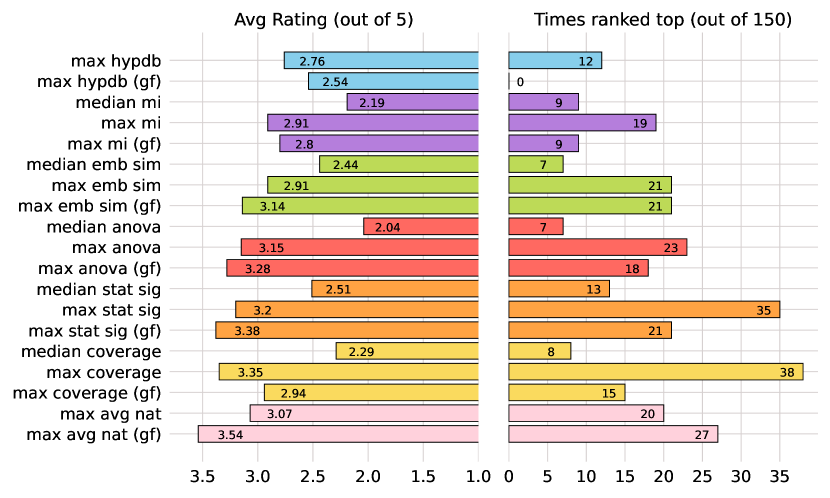
We conclude the following. (1) The refinements in the medians of the measures had significantly lower ratings than their maximum counterparts, hence the naturalness measures coincide with naturalness as perceived by the participants. (2) Maximal $\mathit{Coverage}$ was marked best more times than any other method, followed closely by maximal $\mathit{StatSig}$. The highest average rating belongs to maximal average naturalness with generality filtering. (3) Generality filtering, adapted from OREO (Lin et al., 2022) and applied on each selection method, increased the rating of each method, and statistically significantly for $\mathit{StatSig}$, $\mathit{EmbSim}$ and average naturalness. (4) HypDB responsibility score was significantly lower than max $\mathit{Coverage}$, max $\mathit{StatSig}$ and max average naturalness, which coincides with our observations in our case studies, that HypDB solves a different problem.

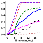
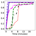
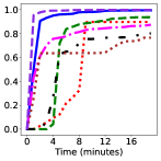
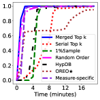
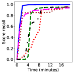
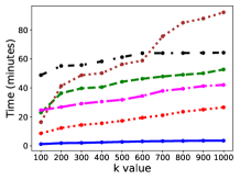
5.4. Effectiveness Evaluation

We compare our methods and external baselines based on score recall over time. Table 4 shows the time till score recall 95% for each prioritization method and naturalness measure. The score recall over time for each naturalness measure for ACS is shown in Figure 1. We focus here on the ACS dataset since it has the largest number of attributes and over 1M rows, and therefore requires the longest run times. Similar trends were seen for the other datasets.

For most of the naturalness measures and datasets, the best method was Merged Top-$k$. In ACS, this method was the first to reach 0.95 recall for $\mathit{MI},\mathit{EmbSim},\mathit{StatSig}$, and the average of all naturalness measures. Over all naturalness measures and all datasets, Merged Top-$k$ was on average 13.4 (and up to 78.3) times faster to reach 0.95 recall than the random-order baseline, and on average 16.2 (up to 82.5) times faster than HypDB. For the Flights dataset, Serial Top-$k$ was the fastest to reach 0.95 recall for all measures except $\mathit{Coverage}$, with Merged Top-$k$ as a close second. The best prioritization for $\mathit{ANOVA}$ was Serial Top-$k$, simply because it is the first measure in the serial order. The external baselines yielded inferior results for all datasets and measures. Prioritizing by HypDB scores performed similarly to random. OREO^⋆ was not applicable to the median query used in stack overflow (since median is not supported in OREO), but on ACS and Flights it was slower to reach 95% recall, if it reached it at all. This is likely because even the enhanced OREO^⋆ version we used operates on a predicate level, which is much more time consuming than our attribute level solution.

The $\mathit{Coverage}$ score recall was the slowest to reach $95\%$ prioritization methods (e.g., over 48 minutes for ACS). This is because $\mathit{Coverage}$ is a predicate-level measure, and the hardest to provide an accurate heuristic for. Our heuristic of prioritizing attribute combinations by their number of large groups hardly predicted large groups that satisfy the user. Still, in Stack Overflow, Merged Top-$k$ was the fastest to reach 95% score recall for $\mathit{Coverage}$. For the ACS dataset, the sampling method with 1% was the fastest, despite the long preprocessing time. We conclude that in the absence of an accurate heuristic for a given measure, sampling can yield fast results, but for naturalness measures with a good predictor (heuristic or pre-computation), Serial Top-$k$ and Merged Top-$k$ prevail.

For the $x$% Sample method we experimented with sample sizes of 1%, 5%, and 10%. The complete set of results is in Appendix A. We observed a trade-off between the time until the first result (which grows with the sample size) and the time until a high score recall (which is shorter for larger samples, as the preliminary search yields more accurate results). However, for most naturalness measures, 1%, so we consider it a recommended sample size. Similar trends were seen for the other datasets, as shown in Table 4.

Due to the results of $x$% Sample on the $\mathit{Coverage}$ measure, one may consider to integrate the sampling method into the Merged Top-$k$ or Serial Top-$k$ methods, as another ranking of the attribute combinations. However, the pre-processing of $x$% Sample will increase the time until high recall is reached in all other measures.

The anytime nature of the algorithm is reflected in that the set of retrieved refinements grows, thus the sum of top-$k$ scores monotonically increases, as seen in Figure 1. In the following experiments, we used this observation to optimize the experimentation time by stopping when the score recall reaches a critical threshold, computed with reference to a full run of the algorithm. When the score recall is not known, one could design an early stopping strategy, based on the size of the change in the top $k$ sum of naturalness scores. For example, “If the $c$ last attribute combinations did not improve the sum of top-$k$ $\nu$ scores by more than $\epsilon$, stop the search”.

Table 4. Time (seconds) to 0.95 score recall and first result time (FRT) for different prioritizations and baselines (OREO^⋆ and HypDB). OREO^⋆ is inapplicable to Stack Overflow as it does not support median aggregation. Entries “t/o” mean that timeout is reached (2 hours for ACS7 and 5 hours for Flights).

Dataset	Prioritization	$\mathit{EmbSim}$	$\mathit{StatSig}$	$\mathit{ANOVA}$	$\mathit{MI}$	$\mathit{Coverage}$	Avg.	FRT
ACS $\alpha=\mathsf{Avg}$	$1$% Sample (3)	1303	300.7	3881	833.3	2886	401	191.0
	$5$% Sample (3)	734	598.7	5733.3	584.33	3720.7	588.3	582.4
	$10$% Sample (3)	1006.3	839.3	3812	830.3	3895.7	834	828.1
	Rand. Order (3)	2914.3	177	5129	909.7	5518.7	1479	10.2
	Serial Top-$k$	3415	554	469	503	4566	1218	84.3
	Merged Top-$k$	231	71	1557	66	4886	76	49.9
	HypDB	1992	290	6079	502	4272	722	139.9
	OREO⋆	5913	1051	t/o	98	t/o	982	38.5
Stack O. $\alpha=\mathsf{Med}$	$1$% Sample (3)	63.3	41.7	298	43.3	332.3	40.7	38.1
	$5$% Sample (3)	77.3	57.7	100.3	54.7	358	55	53.5
	$10$% Sample (3)	94.3	71.7	99.3	70	362.7	70	68.7
	Rand. Order (3)	206.3	9	207.3	313.3	290.7	200	1.1
	Serial Top-$k$	115	9	4	5	246	7	1.8
	Merged Top-$k$	25	7	11	4	206	7	1.9
	HypDB	280	28	313	330	261	203	9.7
Flights $\alpha=\mathsf{Cnt}$	$1$% Sample (3)	133.7	-	131.3	131.3	1022.3	131.3	129.8
	$5$% Sample (3)	261	-	259	259	1148.7	259	257.4
	$10$% Sample (3)	344	-	342	342	1232.7	342	340.4
	Rand. Order (3)	111.7	-	512.7	381.3	793	435.3	20.9
	Serial Top-$k$	37	-	35	35	895	35	34.5
	Merged Top-$k$	40	-	38	38	932	38	34.6
	HypDB	239	-	979	979	928	979	89.9
	OREO⋆	13050	-	t/o	t/o	12298	t/o	12.7

5.5. Parameter Sensitivity

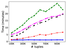
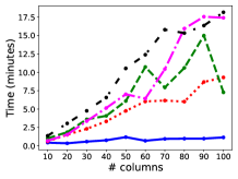
Sensitivity to number of tuples and columns

For the number of tuples (Figure 3a), we sample varying amounts of tuples out of the full ACS dataset. For the number of columns (Figure 3a), we sample increasing sizes of subsets of $\mathrm{SAtt}(D)$ in the ACS dataset. For each number of tuples or columns, we show the average of three runs. We measure the time until a 95% score recall was achieved, for the naturalness measures average score, in each of our five main prioritization methods and in the external baselines - HypDB and OREO^⋆. Similar trends were observed for the other two datasets.

For the naive prioritization of random order and for HypDB, the time until 95% recall steadily rises with the number of tuples or columns. This is also the case for $1$% Sample, since the time to run the pre-processing step of the search on the 1% sample naturally depends on the number of tuples in the database. For OREO^⋆, the time to reach 95% recall was on average 7.8X longer than random order for the number of tuples experiment, and 84X longer for the number of columns experiment. This is due to the predicate level approach taken in OREO^⋆, which does not scale to large datasets. However, for Merged Top-$k$, the time until 95% recall is almost constant. This is due to the prioritization of the search, and covering the most promising attribute combinations at the beginning. For Serial Top-$k$, there is a rise in the time until 95% score recall with the number of tuples or columns, although not as steep as the random order baseline. A possible explanation is that in Serial Top-$k$, only after $k$ refinements for a specific naturalness measure are found, do we continue to the next measure. If there is only a small number of refinements for a specific measure, this may delay the recall for the other measures (and for their average).

Sensitivity to $k$ (number of top refinements)

We measured the time until 95% top-$k$ score recall of the average naturalness measures in the five prioritizations with $k$ values from 100 to 1000 on ACS (Figure 3c). Similar trends were observed on the other datasets. For all methods except Serial Top-$k$, the choice of $k$ does not affect the search algorithm, only the recall computation. For Serial Top-$k$, $k$ refinements are fetched from each naturalness ranking at the beginning of the search. Therefore, for Serial Top-$k$ each point in Figure 3c represents a different algorithm run.

As expected, for all methods the time to 95% recall grows with $k$. However, Merged Top-$k$ exhibited the most subtle rise in time to 95% recall out of all methods (ranging from 1.3 to 3.6 minutes), showing the merit of this combined prioritization method.

(a) Sensitivity to number of tuples

(b) Sensitivity to number of columns

(c) Sensitivity to $k$

(d) Sensitivity to $m$

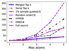
Figure 3. Time for 95% score recall of avg. naturalness over ACS with at most $m=2$ atoms, with varying number of (a) tuples, (b) columns, and (c) varying values of $k$. (d) Sensitivity to maximal number of atoms ($m$): time for 95% recall of average naturalness with increasing number of atoms over Stack Overflow with 10 attributes.

Sensitivity to $m$ (maximal number of attributes per combination)

Increasing $m$ may lead to complex statements, which are less natural. For example, $(\textsf{OpSysProfessional use}{=}\textsf{Windows})\land(\textsf{YearsCode}=0{-}10)\land(\textsf{OrgSize}{=}20{-}99)\land(\textsf{DatabaseHaveWorkedWith}{=}\textsf{MariaDB})\land(\textsf{AccessibilityDifficulties}{=}\textsf{None})$. Most of the refinements with a large $m$ are specializations of a more general refinement (e.g., for stack overflow with 10 attributes, 99.2% of the 44,890 refinements with 5 atoms specialize 3-atom refinements).

While the run times of our algorithms are relatively short, the precomputation times for computing $\mathit{ANOVA}$ and $\mathit{MI}$ in advance were very long (about 24 hours for $m{=}3$). Therefore, we limited this experiment to the 10 attributes responsible for the largest number of refinements retrieved in the 2-atom search. Due to OREO^⋆’s long run times in the previous experiments, it was not included in this experiment. The results are shown in Figure 3d.

As previously, Merged Top-$k$ and Serial Top-$k$ were the fastest to reach 95% recall. For comparison, we added the time to conduct a full claim endorsement search (regardless of the recall level), and as expected, it grows exponentially with $m$. It can be seen that Merged Top-$k$ and Serial Top-$k$ were much faster than that.

6. Related Work

Fact-checking and cherry-picking

Automatic methods to identify cherry-picked results and fake news have been widely studied (Zhou and Zafarani, 2020; Guo et al., 2022; Hassan et al., 2017b). Traditional fact-checking methods rely on domain knowledge (Hassan et al., 2017a, 2015) and lack scalability and persuasiveness without supporting datasets. Other methods employ machine learning and NLP techniques for efficient computational fact-checking (Farinha and Carvalho, 2018; Guo et al., 2022). A considerable body of research focuses on automating fact-checking using structured data (Wu et al., 2014, 2017; Asudeh et al., 2020; Lin et al., 2021; Jo et al., 2019). In one line of work (Wu et al., 2014, 2017), parameterized queries are defined, and the robustness of a fact to parameter perturbations is analyzed. Perturbations are assessed for their relevance and naturalness, depending on the attributes and domain knowledge. In another line of work (Asudeh et al., 2020, 2021), trendlines are examined with respect to their robustness to changes in their start and end points. Cherry-picking has also been examined in rankings (Asudeh et al., 2021), where items are ranked according to a linear combination of numeric attributes, and the weights can be cherry-picked.

Explanations of query answers

Claim endorsement can be viewed as the opposite of the intervention or responsibility approaches in query result explanations (Wu and Madden, 2013; Roy and Suciu, 2014b; Roy et al., 2015; Meliou et al., 2011, 2010, 2014). In the latter, the tuples conforming to a predicate are removed from the database so that the result on the smaller database satisfies a user assertion. Conversely, a predicate in our setting qualifies the tuples that remain in the database to satisfy the user claim. A commonly used type of explanation for query results is a set of predicates that differentiate between tuples in the answer of aggregate queries (El Gebaly et al., 2014; Li et al., 2021; Tao et al., 2022; Roy et al., 2015; Roy and Suciu, 2014b; ten Cate et al., 2015). Our framework similarly provides a ranked list of predicates that define the refinements where the claim holds. However, our primary goal differs in that we seek the most natural refinements to endorse a user’s claim, rather than predicates explaining unexpected query answers. Query refinements have also been used for improving query results according to desired properties (Chapman and Jagadish, 2009), including the number of results (Mishra and Koudas, 2009a; Muslea and Lee, 2005; Koudas et al., 2006; Vélez et al., 1997; Ortega-Binderberger et al., 2002; Mishra and Koudas, 2009b; Chu and Chen, 1994), diversity (Li et al., 2023), or bias removal (Salimi et al., 2018c). We adopt the query refinement approach for the new goal of claim endorsement.

Multidimensional data aggregation

Previous work on multidimensional data aggregation developed methods that extend the traditional drill-down and roll-up operators to find the most interesting data parts for exploration (Agarwal et al., 1996; Sathe and Sarawagi, 2001; Joglekar et al., 2017; Youngmann et al., 2022). Others works have focused on assessing the similarity between two data cubes (Baikousi et al., 2011)). None of these methods corroborate a user’s claim in the aggregate view, or checks whether it represents a meaningful definition of a subpopulation for the claim. Some employ the CUBE operator in SQL (Agarwal et al., 1996), which may seem relevant here to materialize all possible combinations of attributes for refinements. Yet, this approach is not scalable; database systems usually limit the number of attributes in the cube operator to 12 (Salimi et al., 2018b), due to its size being exponential in the number of attributes. It has been shown (Lin et al., 2021) that over 6 attributes, CUBE is impractical for its time and memory consumption.

View Recommendation.

Another relevant area of research has used data aggregations to discover intriguing data visualizations (Vartak et al., 2015; Deutch et al., 2022), with various techniques proposed to recommend the top-$k$ most interesting views (Ehsan et al., 2016; Mafrur et al., 2018; Ding et al., 2019). Some studies recommend visualizations based on visual quality utility functions, such as visual expressiveness (Wongsuphasawat et al., 2015). Others use deviation-based utility functions, where the interestingness of a view is measured by its distance from a reference view (Vartak et al., 2015; Ding et al., 2019; Deutch et al., 2022). Additional studies has explored multi-objective utility functions that capture different aspects of view interestingness (e.g., visual quality, deviation) or aimed to discover the most appropriate utility function for the current analysis context (Ehsan et al., 2016; Mafrur et al., 2018; Zhang et al., 2021). The key distinction from the current work is that interestingness differs significantly from naturalness; in fact, they can be seen as almost opposite concepts. While they seek to identify interesting views that reveal anomalies in the data, our objective is to find the most natural views—those with the fewest special characteristics that do not attract particular attention. The goal is to support claims that hold true across natural subpopulations.

Nonetheless, we share common techniques with this line of work in finding the top-$k$ views. We employ sharing-based optimizations to minimize the number of query executions, similarly to (Vartak et al., 2015), and pruning-based optimizations (like filtering attribute combinations when their maximum group size is too small) to improve running times, as done in (Wongsuphasawat et al., 2015; Vartak et al., 2015). However, given our different objective, we have developed novel optimizations tailored to our specific context.

7. Conclusions and Future Directions

We presented a framework for endorsing user claims through query refinements over the data. Our framework quantifies the quality of a refinement using naturalness measures that have been adapted from the literature but is able to support any measure of naturalness. We proposed an efficient approach for computing refinements using an anytime algorithm with a two-step approach that first produces a ranked list of attribute combinations and then computes value assignments to produce the refinements.

There are multiple avenues of future work that build on this framework. First, it is possible to extend our work to a wider problem definition. Our work currently considers a single relation and can be extended to multi-relation databases, by creating a single view in advance, or by modifying the query for each attribute combination to enable multiple relations. While we focused on refinements (assuming that the claim does not hold in general), ideas in this paper could also be used for relaxations. Attributes combinations can be created from the attributes that appear in the where clause of a given query. The attribute combinations can be prioritized as in Section 4.2 and searched as in Section 4.1. Relaxation for conjunctions appears to be a simpler problem, with the main challenge being prioritization, where our methods also apply. Additionally, an important direction is to enrich the predicate language to inequalities and disjunctions. Inequality predicates can easily be supported in the algorithmic framework, while disjunctions would require changes to the algorithm and different optimizations.

Second, one may consider methods to make the results more accessible to users. For example, one can incorporate desiderata for the ranking of refinements that considers the entire list, such as diversification which would introduce variation in the refinements. This would require designing metrics that combine both naturalness and diversity, and re-ranking the returned refinements while taking the new metric into account. Alternatively, one can consider a summarization strategy for the display of results, grouping similar refinements together and thus facilitating the analysis process.

Third, to make the search process interactive, it would be helpful to develop decision rules that help the user decide when to end the search and could be based on bounds on the quality of potential results. Another intriguing future work is to discover the most suitable naturalness measure in the current analysis context based on user interaction (inspired by (Zhang et al., 2021)).

Finally, our work considers user claims that compare two groups. We intend to consider more elaborate claims such as trends in the query results. This may require considerable adjustment of the problem definition, the predicate space and the algorithm.

Appendix A Sample size for sampling-based search

As mentioned in Section 4.2, we first randomly sample a subset of the dataset and run a fast full claim endorsement search on it. We experimented with 1%, 5% and 10% sample sizes, and we repeat each experiment three times with each sample size. We measure the time until 95% score recall for each naturalness measure in all datasets (shown in the first 3 rows for each dataset in Table 4), and the score recall over time in all naturalness measures for ACS (Figure 4).

We observe a trade-off between the time until first result (which grows with the sample size, due to the preliminary search on the sample) and the time until a high score recall (which is shorter for larger samples, as the preliminary search yields more accurate results). However, for most naturalness measures, $1$% Sample does not fall short behind 5% and 10%. Moreover, for $\mathit{ANOVA}$ and $\mathit{Coverage}$, in the first 20 minutes of the experiment, $1$% Sample reaches the highest score recall. This is likely because for both of these measures, larger sample sizes do not provide additional information that helps predict the score. We conclude that 1% is a good sample size for the tested naturalness measures. Similar trends were seen for the other datasets, as can be seen in Table 4.

(a) $\mathit{ANOVA}$

(b) $\mathit{MI}$

(c) $\mathit{EmbSim}$

(d) $\mathit{Coverage}$

(e) $\mathit{StatSig}$

(f) Average of all

Figure 4. Top 100 score recall for each naturalness measure over time for various sampling sizes in sampling guided search over the ACS dataset.

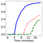
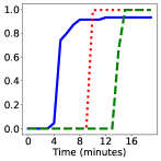
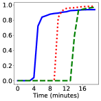
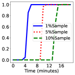
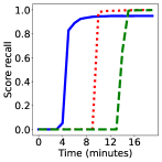
Appendix B Ablation Study

We next isolate several properties of our queries (Section 4.1) and compare them to alternative plausible implementations.

Attribute level vs. predicate level queries.   In our algorithm, we use an attribute level group-by query to search for refinements that endorse the user claim (Section 4.1). It is possible to use a predicate-level query instead and iterate over all possible predicates, as done in the OREO framework (Lin et al., 2021) when searching for counterexamples. In the following experiment, we show that this process is much more time-consuming. The times for a full run of our algorithm with at most one atom ($m=1$) and with a random order of attributes are shown in Table 5 for average and median aggregation functions over two of the datasets. The times in parenthesis are the total SQL times. For average aggregation, the predicate-level search was 10 times slower than the attribute level. For median aggregation, the predicate level search was 5 times slower.

Table 5. Time (SQL time) in seconds for full run of Merged Top-$k$ with at most 1 atom, with random order of attributes.

Dataset	Agg	Predicate level	Attribute level
Stack overflow	Average	48.54 (30.6)	4.48 (1.59)
Stack overflow	Median	49.42 (35.22)	9.32 (6.60)
ACS7	Average	3681 (3578.8)	136 (98.5)
ACS7	Median	4163 (4069.0)	405 (367.17)

Comparison of case-when to join based queries.   The structure of the group-aggregate queries may largely affect the execution time, as it is run for each attribute combination. For example, instead of the CASE-WHEN query in Section 4.1, we could use a naive query with a join: for each group $(g_{1},g_{2})$, compute the values of the aggregation $\alpha$ grouped by the combination of split attributes, and then join the two results by the split attributes.

Table 6. Average and total times in seconds for CASE-WHEN vs. join based queries on ACS with at most $m=2$ atoms.

Aggregation	Run time	CASE-WHEN	join-based
$\alpha=\mathsf{Average}$	Total time	6102 (=1.7 hr)	24081 (=6.7 hr)
	Avg. (std.dev.) time	0.86 (0.1)	3.40 (1.97)
$\alpha=\mathsf{Median}$	Total time	25908 (=7.2 hr)	40256 (=11.2 hr)
	Avg. (std.dev.) time	3.66 (0.35)	5.69 (0.82)

We compare the running times for these two versions of the query on the ACS dataset, with the query about women’s and men’s average/median total income, for $m=2$, i.e., at most two atom predicates (Table 6). Similar trends were observed for other scenarios and thus omitted. Our findings illustrate that employing CASE WHEN queries leads to a consistent and significant improvement in runtime compared to naive join-based queries, particularly for the $\mathsf{Average}$ aggregation function (4x improvement), but also for the $\mathsf{Median}$ aggregation function (1.5x improvement). For example, the average runtime for a single CASE WHEN $\mathsf{Average}$ query was 0.85 seconds, while the average runtime for the corresponding join based queries was 3.4 seconds. This highlights the advantage of utilizing this optimization.

Appendix C User Study Survey

We bring here the instructions and the questions used in our user study.

In this study, you will be asked to rate statements (created based on data) according to how much you would recommend an author to use them. The form takes about 10-15 minutes to fill.

There are 3 topics and in each topic several statements. For each topic, please rate at least one statement as 1 (”Least recommended”) and another one as 5 (”Most recommended”), and rate the others as you see fit. To be considered as ”Most recommended”, the statement should be the best relative to the set of given statements.

The first few questions are meant to provide us with some information about the academic background of study participants. Other than that, no personal information will be saved. Participation is voluntary. You may withdraw at any time, without any negative consequences.

This study is conducted by Shunit Agmon, Benny Kimelfeld, Brit Youngmann and Amir Gilad. For any questions, feel free to contact Shunit Agmon by e-mail: shunit.agmon@gmail.com.

$\boxtimes$ I have reviewed the consent form and agree to participate in this study.

Academic Background

What is you current academic status? (Mark the first option that applies to you).
$\boxtimes$ Pursuing a graduate degree (master’s or PhD)
$\boxtimes$ Pursuing a bachelor’s degree
$\boxtimes$I have a PhD
$\boxtimes$I have a Master’s degree
$\boxtimes$I have a Bachelor’s degree
$\boxtimes$Not pursuing a degree
What is your major or field of study? (open question)

Flight Delays on Mondays vs. Saturdays

Alice is writing a traveling blog recommending her readers to prefer flights on Mondays over Saturdays to minimize delays. She has the statements below, based on US flight delays records from 2015. To what extent would you recommend to Alice to use each of them in her article?

Please rate at least one statement as “Least recommended” and another one as “Most recommended”, and rate the others as you see fit (2 statements can get the same score).

• Among flights scheduled to depart between 3:00-4:00 AM, there are more delays on Saturdays (43) vs. Mondays (30).

• Among flights with flight number 2, there are more delays on Saturdays (49) vs. Mondays (48).

• Among flights operated by Hawaiian Airlines Inc., there are more delays on Saturdays (1,028) vs. Mondays (986).

• In October, there were more flight delays on Saturdays (9,549) vs. Mondays (8,744).

• Among flights with flight number 3507, there were more flight delays on Saturdays (13) vs. Mondays (10).

• Among flights with flight number 3430, there were more flight delays on Saturdays (16) vs. Mondays (14).

• Among flights with flight number 4876, there were more flight delays on Saturdays (14) vs. Mondays (9).

• Among flights with air time between 390 and 400 minutes, there were more flight delays on Saturdays (51) vs. Mondays (41).

• Among flights on the last days of the month (30-31), there were more flight delays on Saturdays (3,753) vs. Mondays (2,573).

• Among flights with scheduled duration between 480 and 490 minutes, there were more flight delays on Saturdays (17) vs. Mondays (14).

Before you continue to the next section… please make sure that in the previous section, you have rated at least one of the statements as 5 (most recommended) and at least one of the statements as 1 (least recommended).

Master’s vs. Bachelor’s Salary

Bella is writing a article about the salary benefits of a Master’s degree. She has the statements below, drawn from the 2022 StackOverflow Developer’s Survey. To what extent would you recommend to Bella to use each of them in her article?

Please rate at least one statement as ”Least recommended” and another one as ”Most recommended”, and rate the others as you see fit (2 statements can get the same score).

• Among the 174 people (out of 38K) in Iran who have been professionally coding for under 10 years, MSc graduates earn a higher salary on average ($56K) than BSc graduates ($39K).

• Among the 40 People (out of 38K) in Croatia who have been coding for under 10 years, MSc graduates earn a higher salary on average ($46K) than BSc graduates ($22K).

• Among the 4,525 people (out of 38K) who use Linux based operating systems and have been coding for up to 10 years, MSc graduates earn a higher salary on average ($134K) than BSc graduates ($121K).

• Among the 234 people (out of 38K) who want to work with Bash/Shell language and decide what new tools to buy by asking developers they know, MSc graduates earn a higher salary on average ($313K) than BSc graduates ($197K).

• Among the 280 people (out of 38K) who define themselves as Southeast Asian, MSc graduates earn a higher salary on average ($83K) than BSc graduates ($42K).

• Among the 40 people (out of 38K) in Croatia who have up to 10 years of work experience, MSc graduates earn a higher salary on average ($46K) than BSc graduates ($30K).

• Among the 10,698 people (out of 38K) who use Linux based operating systems, MSc graduates earn a higher salary on average ($167K) than BSc graduates ($166K).

• Among the 16 people (out of 38K) who want to work with PyCharm and learn to code through online courses, MSc graduates earn a higher salary on average ($54.7K) than BSc graduates ($13.5K).

• Among the 687 people (out of 38K) who are independent or freelancers and have been coding for 10 to 20 years, MSc graduates earn a higher salary on average ($145K) than BSc graduates ($100K).

• Among the 836 people (out of 38K) who have 20-30 years of work experience, MSc graduates earn a higher salary on average ($256K) than BSc graduates ($225K).

• Among the 2049 people (out of 38K) who work in India, MSc graduates earn a higher salary on average ($52.5K) than BSc graduates ($51.6K).

• Among the 1442 people (out of 38K) who decide what new tools to buy by asking developers they know, MSc graduates earn a higher salary on average ($182K) than BSc graduates ($166K).

• Among the 1872 people (out of 38K) who work in Germany, MSc graduates earn a higher salary on average ($135K) than BSc graduates ($114K).

• Among the 22 people (out of 38K) who have worked with OpenStack platform and would like to work with Microsoft Teams, MSc graduates earn a higher salary on average ($98K) than BSc graduates ($48K).

• Among the 32 people (out of 38K) who have worked with Notepad++ and do not know the size of their organization, MSc graduates earn a higher salary on average ($231K) than BSc graduates ($62K).

• Among the 27 people (out of 38K) who have worked with Jira and want to work with Rocketchat, MSc graduates earn a higher salary on average ($160K) than BSc graduates ($75K).

• Among the 60 people (out of 38K) who define themselves as Indian and want to work with Vim, MSc graduates earn a higher salary on average ($160K) than BSc graduates ($75K).

• Among the 308 people (out of 38K) who use Windows operating system and have worked with the Express web framework, MSc graduates earn a higher salary on average ($180K) than BSc graduates ($103K).

Before you continue to the next section… please make sure that in the previous section, you have rated at least one of the statements as 5 (most recommended) and at least one of the statements as 1 (least recommended).

Women’s vs. Men’s Income

Charlotte is writing an article about women’s income being higher than is commonly expected. Note the difference between income and salary: it is possible to get an income without being employed (e.g., from various support sources or passive income from investments). She has the statements below, drawn from the US Census survey of 2018 in the largest seven states in the US. To what extent would you recommend to Charlotte to use each of them in her article?

Please rate at least one statement as ”Least recommended” and another one as ”Most recommended”, and rate the others as you see fit (2 statements can get the same score).

• Among the 930 (out of 1.2M) 12th grade students who have last worked 1-5 years ago, women have a higher income on average ($2,768) than men ($1,656).

• Among the 28,366 people (out of 1.2M) with insurance through an employer or union, who have a child, women have a higher income on average ($1,044) than men ($1,017).

• Among the 49,011 (out of 1.2M) African Americans who were never married, women have a higher income on average ($21.5K) than men ($16.7K).

• Among the 582 (out of 1.2M) army veterans who have not reported a Veteran Service Disability Rating and who do not have cognitive difficulty, women have a higher income on average ($57K) than men ($46K).

• Among the 730 (out of 1.2M) army veterans who have not reported a Veteran Service Disability Rating, women have a higher income on average ($50K) than men ($43K).

• Among the 129,462 people (out of 1.2M) who are not in the labor force and were never married, women have a higher income on average ($7,325) than men ($7,201).

• Among the 7,595 people (out of 1.2M) who work for a private company and have a child, women have a higher income on average ($3,474) than men ($3,436).

• Among the 1,599 people (out of 1.2M) of age 20-30 who work in the armed forces, women have a higher income on average ($39K) than men ($37K).

• Among the 91K people (out of 1.2M) who were never married and have not worked in the last 5 years, women have a higher income on average ($6,155) than men ($5,649).

• Among the 118 people (out of 1.2M) who depart for work between 6:45-7:35 and work as producers and directors, women have a higher income on average ($105K) than men ($98K).

• Among the 9,892 people (out of 1.2M) who do not have health insurance and work in construction, women have a higher income on average ($29K) than men ($28K).

• Among the 583 people (out of 1.2M) who work as paralegals and legal assistants in west US, women have a higher income on average ($60K) than men ($58K).

• Among the 174 African American people (out of 1.2M) in Polk county (Florida), women have a higher income on average ($22K) than men ($15K).

• Among the 86 people who define themselves as White (out of 1.2M) who were born in Vietnam, women have a higher income on average ($51K) than men ($43K).

Before you finish… please make sure that in the previous section, you have rated at least one of the statements as 5 (most recommended) and at least one of the statements as 1 (least recommended).

References

- (1)
- Agarwal et al. (1996) Sameet Agarwal, Rakesh Agrawal, Prasad Deshpande, Ashish Gupta, Jeffrey F. Naughton, Raghu Ramakrishnan, and Sunita Sarawagi. 1996. On the Computation of Multidimensional Aggregates. In VLDB. Morgan Kaufmann, 506–521.
- Asudeh et al. (2020) Abolfazl Asudeh, Hosagrahar Visvesvaraya Jagadish, You Wu, and Cong Yu. 2020. On detecting cherry-picked trendlines. VLDB 13, 6 (2020), 939–952.
- Asudeh et al. (2021) Abolfazl Asudeh, You Will Wu, Cong Yu, and HV Jagadish. 2021. Perturbation-based Detection and Resolution of Cherry-picking. A Quarterly bulletin of the Computer Soc. of the IEEE Technical Committee on Data Engineering 45, 3 (2021).
- Baikousi et al. (2011) Eftychia Baikousi, Georgios Rogkakos, and Panos Vassiliadis. 2011. Similarity measures for multidimensional data. In 2011 IEEE 27th International Conference on Data Engineering. IEEE, 171–182.
- Borrego et al. (2018) Maura Borrego, David B Knight, Kenneth Gibbs Jr, and Erin Crede. 2018. Pursuing graduate study: Factors underlying undergraduate engineering students’ decisions. Journal of Engineering Education 107, 1 (2018), 140–163.
- Caliskan et al. (2017) Aylin Caliskan, Joanna J Bryson, and Arvind Narayanan. 2017. Semantics derived automatically from language corpora contain human-like biases. Science 356, 6334 (2017), 183–186.
- Chapman and Jagadish (2009) Adriane Chapman and HV Jagadish. 2009. Why not?. In Proceedings of the 2009 ACM SIGMOD International Conference on Management of data. 523–534.
- Chu and Chen (1994) Wesley W. Chu and Qiming Chen. 1994. A structured approach for cooperative query answering. IEEE Transactions on Knowledge and Data Engineering 6, 5 (1994), 738–749.
- Deutch et al. (2022) Daniel Deutch, Amir Gilad, Tova Milo, Amit Mualem, and Amit Somech. 2022. FEDEX: An Explainability Framework for Data Exploration Steps. VLDB 15, 13 (2022), 3854–3868.
- Ding et al. (2021) Frances Ding, Moritz Hardt, John Miller, and Ludwig Schmidt. 2021. Retiring Adult: New Datasets for Fair Machine Learning. Advances in Neural Information Processing Systems 34 (2021).
- Ding et al. (2019) Rui Ding, Shi Han, Yong Xu, Haidong Zhang, and Dongmei Zhang. 2019. Quickinsights: Quick and automatic discovery of insights from multi-dimensional data. In Proceedings of the 2019 international conference on management of data. 317–332.
- Ehsan et al. (2016) Humaira Ehsan, Mohamed A Sharaf, and Panos K Chrysanthis. 2016. Muve: Efficient multi-objective view recommendation for visual data exploration. In 2016 IEEE 32nd International Conference on Data Engineering (ICDE). IEEE, 731–742.
- El Gebaly et al. (2014) Kareem El Gebaly, Parag Agrawal, Lukasz Golab, Flip Korn, and Divesh Srivastava. 2014. Interpretable and informative explanations of outcomes. Proceedings of the VLDB Endowment 8, 1 (2014), 61–72.
- Farinha and Carvalho (2018) Hugo Farinha and Joao P Carvalho. 2018. Towards computational fact-checking: Is the information checkable?. In fuzz-IEEE. IEEE, 1–7.
- Galhotra et al. (2021) Sainyam Galhotra, Romila Pradhan, and Babak Salimi. 2021. Explaining Black-Box Algorithms Using Probabilistic Contrastive Counterfactuals. In SIGMOD. ACM, 577–590.
- Guo et al. (2022) Zhijiang Guo, Michael Schlichtkrull, and Andreas Vlachos. 2022. A survey on automated fact-checking. TACL 10 (2022), 178–206.
- Hassan et al. (2017a) Naeemul Hassan, Fatma Arslan, Chengkai Li, and Mark Tremayne. 2017a. Toward automated fact-checking: Detecting check-worthy factual claims by claimbuster. In KDD. 1803–1812.
- Hassan et al. (2015) Naeemul Hassan, Chengkai Li, and Mark Tremayne. 2015. Detecting check-worthy factual claims in presidential debates. In CIKM. 1835–1838.
- Hassan et al. (2017b) Naeemul Hassan, Gensheng Zhang, Fatma Arslan, Josue Caraballo, Damian Jimenez, Siddhant Gawsane, Shohedul Hasan, Minumol Joseph, Aaditya Kulkarni, Anil Kumar Nayak, et al. 2017b. Claimbuster: The first-ever end-to-end fact-checking system. VLDB 10, 12 (2017), 1945–1948.
- Järvelin and Kekäläinen (2002) Kalervo Järvelin and Jaana Kekäläinen. 2002. Cumulated gain-based evaluation of IR techniques. TOIS 20, 4 (2002), 422–446.
- Jo et al. (2019) Saehan Jo, Immanuel Trummer, Weicheng Yu, Xuezhi Wang, Cong Yu, Daniel Liu, and Niyati Mehta. 2019. Aggchecker: A fact-checking system for text summaries of relational data sets. VLDB 12, 12 (2019), 1938–1941.
- Joglekar et al. (2017) Manas Joglekar, Hector Garcia-Molina, and Aditya Parameswaran. 2017. Interactive data exploration with smart drill-down. IEEE Transactions on Knowledge and Data Engineering 31, 1 (2017), 46–60.
- Kandel et al. (2012) Sean Kandel, Ravi Parikh, Andreas Paepcke, Joseph M Hellerstein, and Jeffrey Heer. 2012. Profiler: Integrated statistical analysis and visualization for data quality assessment. In AVI. 547–554.
- Kanji (2006) Gopal K Kanji. 2006. 100 Statistical Tests. SAGE Publications.
- Karagiannis et al. (2020) Georgios Karagiannis, Mohammed Saeed, Paolo Papotti, and Immanuel Trummer. 2020. Scrutinizer: fact checking statistical claims. Proceedings of the VLDB Endowment 13, 12 (2020), 2965–2968.
- Karimi et al. (2023) Amir-Hossein Karimi, Gilles Barthe, Bernhard Schölkopf, and Isabel Valera. 2023. A Survey of Algorithmic Recourse: Contrastive Explanations and Consequential Recommendations. ACM Comput. Surv. 55, 5 (2023), 95:1–95:29.
- Karimi et al. (2021) Amir-Hossein Karimi, Bernhard Schölkopf, and Isabel Valera. 2021. Algorithmic Recourse: from Counterfactual Explanations to Interventions. In FAccT. ACM, 353–362.
- Kendall (1938) Maurice G Kendall. 1938. A new measure of rank correlation. Biometrika 30, 1/2 (1938), 81–93.
- Koudas et al. (2006) Nick Koudas, Chen Li, Anthony K. H. Tung, and Rares Vernica. 2006. Relaxing Join and Selection Queries. In VLDB. ACM, 199–210.
- Li et al. (2021) Chenjie Li, Zhengjie Miao, Qitian Zeng, Boris Glavic, and Sudeepa Roy. 2021. Putting things into context: Rich explanations for query answers using join graphs. In SIGMOD. 1051–1063.
- Li et al. (2023) Jinyang Li, Yuval Moskovitch, Julia Stoyanovich, and H. V. Jagadish. 2023. Query Refinement for Diversity Constraint Satisfaction. VLDB 17, 2 (2023), 106–118.
- Lin et al. (2021) Yin Lin, Brit Youngmann, Yuval Moskovitch, HV Jagadish, and Tova Milo. 2021. On detecting cherry-picked generalizations. VLDB 15, 1 (2021), 59–71.
- Lin et al. (2022) Yin Lin, Brit Youngmann, Yuval Moskovitch, HV Jagadish, and Tova Milo. 2022. OREO: detection of cherry-picked generalizations. Proceedings of the VLDB Endowment 15, 12 (2022), 3570–3573.
- Ma et al. (2023) Pingchuan Ma, Rui Ding, Shuai Wang, Shi Han, and Dongmei Zhang. 2023. XInsight: EXplainable Data Analysis Through The Lens of Causality. Proc. ACM Manag. Data, Article 156 (jun 2023), 27 pages.
- Mafrur et al. (2018) Rischan Mafrur, Mohamed A Sharaf, and Hina A Khan. 2018. Dive: Diversifying view recommendation for visual data exploration. In Proceedings of the 27th ACM International Conference on Information and Knowledge Management. 1123–1132.
- Meliou et al. (2010) Alexandra Meliou, Wolfgang Gatterbauer, Katherine F. Moore, and Dan Suciu. 2010. The Complexity of Causality and Responsibility for Query Answers and non-Answers. Proc. VLDB Endow. 4, 1 (2010), 34–45.
- Meliou et al. (2011) Alexandra Meliou, Wolfgang Gatterbauer, Suman Nath, and Dan Suciu. 2011. Tracing data errors with view-conditioned causality. In SIGMOD. ACM, 505–516.
- Meliou et al. (2014) Alexandra Meliou, Sudeepa Roy, and Dan Suciu. 2014. Causality and Explanations in Databases. Proc. VLDB Endow. 7, 13 (2014), 1715–1716.
- Miao et al. (2019) Zhengjie Miao, Qitian Zeng, Boris Glavic, and Sudeepa Roy. 2019. Going beyond provenance: Explaining query answers with pattern-based counterbalances. In Proceedings of the 2019 International Conference on Management of Data. 485–502.
- Mishra and Koudas (2009a) Chaitanya Mishra and Nick Koudas. 2009a. Interactive query refinement. In EDBT (ACM International Conference Proceeding Series), Vol. 360. ACM, 862–873.
- Mishra and Koudas (2009b) Chaitanya Mishra and Nick Koudas. 2009b. Interactive query refinement. In Proceedings of the 12th International Conference on Extending Database Technology: Advances in Database Technology. 862–873.
- Muslea and Lee (2005) Ion Muslea and Thomas J Lee. 2005. Online query relaxation via bayesian causal structures discovery. In AAAI. 831–836.
- Ortega-Binderberger et al. (2002) Michael Ortega-Binderberger, Kaushik Chakrabarti, and Sharad Mehrotra. 2002. An Approach to Integrating Query Refinement in SQL. In EDBT (Lecture Notes in Computer Science), Vol. 2287. Springer, 15–33.
- Pradhan et al. (2022) Romila Pradhan, Jiongli Zhu, Boris Glavic, and Babak Salimi. 2022. Interpretable Data-Based Explanations for Fairness Debugging. In SIGMOD. ACM, 247–261.
- Reimers and Gurevych (2019) Nils Reimers and Iryna Gurevych. 2019. Sentence-BERT: Sentence Embeddings using Siamese BERT-Networks. In EMNLP/IJCNLP (1). Association for Computational Linguistics, 3980–3990.
- Roy et al. (2015) Sudeepa Roy, Laurel Orr, and Dan Suciu. 2015. Explaining query answers with explanation-ready databases. VLDB 9, 4 (2015), 348–359.
- Roy and Suciu (2014a) Sudeepa Roy and Dan Suciu. 2014a. A formal approach to finding explanations for database queries. In SIGMOD. ACM, 1579–1590.
- Roy and Suciu (2014b) Sudeepa Roy and Dan Suciu. 2014b. A formal approach to finding explanations for database queries. In Proceedings of the 2014 ACM SIGMOD international conference on Management of data. 1579–1590.
- Salimi et al. (2018a) Babak Salimi, Corey Cole, Peter Li, Johannes Gehrke, and Dan Suciu. 2018a. HypDB: a demonstration of detecting, explaining and resolving bias in OLAP queries. Proceedings of the VLDB Endowment 11, 12 (2018), 2062–2065.
- Salimi et al. (2018b) Babak Salimi, Johannes Gehrke, and Dan Suciu. 2018b. Bias in OLAP Queries: Detection, Explanation, and Removal. In SIGMOD. 1021–1035.
- Salimi et al. (2018c) Babak Salimi, Johannes Gehrke, and Dan Suciu. 2018c. Bias in OLAP Queries: Detection, Explanation, and Removal. In SIGMOD. ACM, 1021–1035.
- Sathe and Sarawagi (2001) Gayatri Sathe and Sunita Sarawagi. 2001. Intelligent rollups in multidimensional OLAP data. In VLDB. ResearchGate GmbH, 307–316.
- Sprent and Smeeton (2007) Peter Sprent and Nigel C Smeeton. 2007. Applied nonparametric statistical methods. CRC press, Chapter 5, 86–111.
- Tang et al. (2017) Bo Tang, Shi Han, Man Lung Yiu, Rui Ding, and Dongmei Zhang. 2017. Extracting top-k insights from multi-dimensional data. In Proceedings of the 2017 ACM International Conference on Management of Data. 1509–1524.
- Tao et al. (2022) Yuchao Tao, Amir Gilad, Ashwin Machanavajjhala, and Sudeepa Roy. 2022. DPXPlain: Privately Explaining Aggregate Query Answers. Proc. VLDB Endow. 16, 1 (2022), 113–126. https://doi.org/10.14778/3561261.3561271
- ten Cate et al. (2015) Balder ten Cate, Cristina Civili, Evgeny Sherkhonov, and Wang-Chiew Tan. 2015. High-level why-not explanations using ontologies. In PODS. 31–43.
- Vandenbroucke (2018) Guillaume Vandenbroucke. 2018. Married men sit atop the wage ladder. Economic Synopses 24 (2018).
- Vartak et al. (2015) Manasi Vartak, Sajjadur Rahman, Samuel Madden, Aditya Parameswaran, and Neoklis Polyzotis. 2015. Seedb: Efficient data-driven visualization recommendations to support visual analytics. In VLDB, Vol. 8. NIH Public Access, 2182.
- Vélez et al. (1997) Bienvenido Vélez, Ron Weiss, Mark A. Sheldon, and David K. Gifford. 1997. Fast and Effective Query Refinement. In SIGIR. ACM, 6–15.
- Wasserman (2004) Larry Wasserman. 2004. All of statistics: a concise course in statistical inference. Vol. 26. Springer.
- Wongsuphasawat et al. (2015) Kanit Wongsuphasawat, Dominik Moritz, Anushka Anand, Jock Mackinlay, Bill Howe, and Jeffrey Heer. 2015. Voyager: Exploratory analysis via faceted browsing of visualization recommendations. IEEE transactions on visualization and computer graphics 22, 1 (2015), 649–658.
- Wu and Madden (2013) Eugene Wu and Samuel Madden. 2013. Scorpion: Explaining Away Outliers in Aggregate Queries. Proc. VLDB Endow. 6, 8 (2013), 553–564.
- Wu et al. (2009) Tianyi Wu, Dong Xin, Qiaozhu Mei, and Jiawei Han. 2009. Promotion analysis in multi-dimensional space. VLDB 2, 1 (2009), 109–120.
- Wu et al. (2014) You Wu, Pankaj K Agarwal, Chengkai Li, Jun Yang, and Cong Yu. 2014. Toward computational fact-checking. Proceedings of the VLDB Endowment 7, 7 (2014), 589–600.
- Wu et al. (2017) You Wu, Pankaj K Agarwal, Chengkai Li, Jun Yang, and Cong Yu. 2017. Computational fact checking through query perturbations. ACM Transactions on Database Systems (TODS) 42, 1 (2017), 1–41.
- Yates (1934) Frank Yates. 1934. Contingency tables involving small numbers and the test. Supplement to the Journal of the Royal Statistical Society 1, 2 (1934), 217–235.
- Youngmann et al. (2022) Brit Youngmann, Sihem Amer-Yahia, and Aurélien Personnaz. 2022. Guided Exploration of Data Summaries. Proc. VLDB Endow. 15, 9 (2022), 1798–1807.
- Youngmann et al. (2023) Brit Youngmann, Michael Cafarella, Yuval Moskovitch, and Babak Salimi. 2023. On Explaining Confounding Bias. In ICDE. IEEE, 1846–1859.
- Zhang et al. (2021) Xiaozhong Zhang, Xiaoyu Ge, Panos K Chrysanthis, and Mohamed A Sharaf. 2021. Viewseeker: An interactive view recommendation framework. Big Data Research 25 (2021), 100238.
- Zhou and Zafarani (2020) Xinyi Zhou and Reza Zafarani. 2020. A survey of fake news: Fundamental theories, detection methods, and opportunities. ACM Computing Surveys (CSUR) 53, 5 (2020), 1–40.
- Zilberstein (1996) Shlomo Zilberstein. 1996. Using anytime algorithms in intelligent systems. AI magazine 17, 3 (1996), 73–73.