A little bit of self-correction

Abstract

We investigate the emergence of stable subspaces in the low-temperature quantum thermal dynamics of finite spin chains. Our analysis reveals the existence of effective decoherence-free qudit subspaces, persisting for timescales exponential in $\beta$. Surprisingly, the appearance of metastable subspaces is not directly related to the entanglement structure of the ground state(s). Rather, they arise from symmetry relations in low-lying excited states. Despite their stability within a ’phase’, practical realization of stable qubits is hindered by susceptibility to symmetry-breaking perturbations. This work highlights that there can be non-trivial quantum behavior in the thermal dynamics of noncommuting many body models, and opens the door to more extensive studies of self-correction in such systems.

I Introduction

The pursuit of a self-correcting quantum memory, while still largely elusive, has been an exceptionally fertile ground for identifying new approaches to robustly process quantum information Brown et al. (2016); Kitaev (2003); Bombín (2015a); Bacon (2006); Haah (2011); Kastoryano and Brandao (2016a); Bombín (2015b); Nathan et al. (2024). Ideally, a self-correcting quantum memory would be a system that inherently stabilizes itself against thermal, stochastic and coherent noise. A less stringent, yet still valuable, form involves a qubit subspace that is robust against thermal fluctuations but may not withstand arbitrary non-thermal perturbations. At present most of our understanding of thermal stability is based on commuting models Alicki et al. (2009, 2010), mostly because, until recently, no reliable mathematical model existed for studying the thermalization of noncommuting many body systems.

The interplay between quantum mechanics and statistical mechanics becomes particularly intriguing at low temperatures. While the high-temperature behavior of non-commuting systems tends to mimic classical Gibbs states Bakshi et al. (2024); Rouzé et al. (2024), low temperatures reveal a richer structure. The characteristics of the low-lying quantum states, particularly entanglement, intertwine with the statistical features of the Gibbs distribution. When the temperature is lower than the spectral gap, we expect the Gibbs state to approximate the ground state, suggesting that the quantum thermal dynamics should mirror the properties of the ground state. This leads to the hypothesis that the mixing time – the timescale over which the system reaches thermal equilibrium – might diverge at a quantum phase transition at low temperatures. Such a hypothesis would be consistent with the statics-dynamics connection that is well studied for classical spin systems Martinelli (1999) and commuting quantum spin systems Kastoryano and Brandao (2016a); Capel et al. (2020).

Building on the new quasi-local noncommutative Gibbs samplers constructed in Refs. Chen et al. (2023a, b); Gilyén et al. (2024); Ding et al. (2024), we investigate the low-temperature quantum thermal dynamics of a specific class of one-parameter quantum spin chains: the $J_{1}-J_{2}$ chain. Spin chains are notable as they lack a thermal phase transitions, yet they undergo quantum phase transitions Sachdev (1999). Our analysis reveals that: (i) There exist qudit subspaces that remain decoherence-free for timescales on the order of $\Omega(N^{-1}e^{\beta c})$, where $\beta$ is the inverse temperature and $c$ is a constant related to gaps in the low lying spectrum of the Hamiltonian and $N$ is the chain length. (ii) The existence of metastable subspaces does not require ground state degeneracy of the model. Rather, it originates from symmetry constraints in the low lying spectrum, and depends on the system-bath coupling operators. (iii) The ’phase diagram’ of these stable subspaces does not necessarily mirror the ground state quantum phase diagram. Instead, the metastable subspaces can appear and disappear at (avoided-)crossings of the low-lying excited states of the model (see Fig. 1).

Despite the intriguing nature of these findings, we temper expectations as for their practical utility in building noise resilient qubits. The primary limitation stems from the protection mechanism’s reliance on discrete symmetries. Such symmetries are vulnerable to local perturbations, which can easily disrupt the stability afforded by these decoherence-free subspaces. Consequently, while the stable subspaces reveal interesting new physics in the thermal dynamics of quantum systems, they may not translate into practical, fault-tolerant quantum memories.

This work is significant for several reasons. First, it provides initial evidence of non-trivial quantum behavior of thermalization. This marks a departure from the classical understanding, showcasing how quantum effects can alter thermal dynamics in unexpected ways. Second, it highlights the critical influence of the choice of elementary jump operators on the system’s dynamics. This observation suggests that subtle details in the model’s implementation can have profound impacts on its behavior. Finally, the presence of approximate decoherence-free subspaces within the thermal dynamics of spin systems suggests that such phenomena might be more common than previously thought, opening new avenues for exploring the interplay between quantum coherence and thermal noise.

II Metastability

While ground states of commuting Hamiltonians always have finite correlation length, noncommuting quantum many body systems can extensive ground state correlations, allowing for various forms of topological and symmetry driven quantum phase transitions Sachdev (1999); Zeng et al. (2019). While the quantum thermal dynamics of commuting systems is fairly well understood Kastoryano and Brandao (2016b); Bardet et al. (2023), the quantum thermal dynamics of noncommuting many body systems is essentially uncharted territory. This is due in large part to the lack of a go-to quantum thermal dynamics algorithm. Recently, a subset of the authors introduced a (quasi)-local quantum Lindbladian that satisfies detailed balance with respect to a noncommuting quantum Gibbs state Chen et al. (2023b), hence allowing for the analytic and numerical analysis of quantum Gibbs sampling. This new construction will be the starting point for our analysis.

We consider a quantum system described by a local many body Hamiltonian $H$, on a regular lattice $\Lambda$. The thermal Markovian dynamics elaborated in Refs. Chen et al. (2023a, b); Gilyén et al. (2024); Ding et al. (2024) is defined by a Lindbladian (the generator of a quantum dynamical semigroup)

$$\mathcal{L}(\rho)=-i[Q,\rho]+\sum_{a}L_{a}\rho L_{a}^{\dagger}-\frac{1}{2}(L_{a}^{\dagger}L_{a}\rho+\rho L_{a}^{\dagger}L_{a}).$$ (1)

$L_{a}$ are the quantum jumps, or Lindblad operators, and are given explicitly by

$$L_{a}=\int_{-\infty}^{\infty}g(t)e^{-itH}S_{a}e^{itH}dt,$$ (2)

where $\{S_{a}\}$ are a complete set of elemental jump operators that guarantee ergodicity of the dynamics. In the case of a quantum spin model on a 1D lattice (a ring), it is customary to choose $\{S_{a}\}$ to be the set of local Pauli operators: $S_{a}\in\{X_{n},Y_{n},Z_{n}\}_{n\in\Lambda}$. $g(t)=\int_{-\infty}^{\infty}\sqrt{\gamma(\omega)}e^{it\omega}d\omega$, is a damping term, and $\gamma(\omega)$ is related to the bath auto-correlation function, and incorporates the system bath coupling strength. For concreteness, we assume that $\gamma(\omega)\propto 1/(1+e^{\beta\omega})$ for a specific temperature $\beta$. This choice is reminiscent of an Ohmic bath Gardiner and Zoller (2004), but all of our conclusions hold more generally, as long as $\gamma(-\omega)=e^{\beta\omega}\gamma(\omega)$. We choose to work with the specific form of jump operators in Eqn. (2) for concreteness, however there is a wider class of constructions which lead to the same conclusions Gilyén et al. (2024); Ding et al. (2024).

$Q$ is a Hermitian matrix, playing the role of the system Hamiltonian. The two natural candidates for $Q$ are (i) $Q\propto H$, the Hamiltonian of the system, and (ii)

$$Q=\frac{i}{2}\sum_{ij}\tanh\left(\frac{\beta(e_{i}-e_{j})}{4}\right)\langle e_{i}|\sum_{a}L_{a}^{\dagger}L_{a}|e_{j}\rangle|e_{i}\rangle\langle e_{j}|,$$ (3)

written out in the eigenbasis of $H=\sum_{j}e_{j}|e_{j}\rangle\langle e_{j}|$. The latter choice guarantees that the stationary state of the dissipative dynamics is the Gibbs state; i.e. $\mathcal{L}(\rho_{\beta})=0$ with $\rho_{\beta}\propto e^{-\beta H}$. The specific form in Eqn. (3) is necessary to enforce the quantum detailed balance condition Chen et al. (2023b); Gilyén et al. (2024); Ding et al. (2024) – the key mathematical relationship governing both classical and quantum Gibbs samplers. The first choice $Q=H$ is closer to the natural dynamics resulting from a Markovian weak coupling limit, as shown in Ref. Nathan and Rudner (2020). However, it does not lead to a stationary state that is globally Gibbs at any temperature. We will see that at low enough temperatures both choices lead to metastable quantum subspaces, though $Q=H$ induces coherent dynamics in the metastable subspace.

It is worth pausing at this point to discuss how important the choice of bath couplers $\{S_{a}\}$ is for the thermalization process. By analogy with the classical Metropolis algorithm, it is generally believed that as long as the operators $\{S_{a}\}$ are local on the lattice, and span the full algebra of the space, then the dynamics will not depend sensitively on the specific choice of couplers $\{S_{a}\}$. This intuition builds upon a deep correspondence from Glauber dynamics of classical spin systems, which shows a complete correspondence between static properties of the Gibbs sates and the mixing time of the dynamics Martinelli (1999). We show, on the contrary, that the choice of couplers plays a crucial role in the quantum case in the large $\beta$ limit, when the statics is dominated by the ground state.

Decoherence-free subspaces

We say that a Lindbladian admits a decoherence-free subspace (DFS) $\mathcal{D}$ if for any state $\psi\in\mathcal{D}$, $\mathcal{L}(\psi)=0$ Knill et al. (2000); Zanardi (2000). Equivalently Kraus et al. (2008), $\mathcal{D}$ is a DFS of $\mathcal{L}$ if $L_{a}|\psi\rangle=0$ and $Q|\psi\rangle\propto|\psi\rangle$, for all Kraus operators $L_{a}$, and any pure state $|\psi\rangle\in\mathcal{D}$. We will consider an $\epsilon$-approximate version of the DFS ($\epsilon$-DFS):

$$||L_{a}|\psi\rangle|| \leq \epsilon||L_{a}||$$ (4)

$$||Q|\psi\rangle|| \leq \epsilon||H||.$$ (5)

In general, the Hamiltonian only needs $|\psi\rangle$ to be an approximate eigenstate for the subspace to be $\epsilon$-DFS, but for our purpose, the more restrictive definition is sufficient.

Definition II.1 (Blind qubit subspace)

Consider a Hamiltonian $H=\sum_{j}e_{j}|e_{j}\rangle\langle e_{j}|$, with its eigenvalues in increasing order: $e_{0}\leq e_{1}\leq...$, and a set of elemental jump operators $\{S_{a}\}$. If there exists an eigenvector $|e_{k}\rangle$, $k>0$ such that $\langle e_{j}|S_{a}|e_{k}\rangle=0$ for all $j\leq k$, and $\langle e_{0}|S_{a}|e_{0}\rangle=0$, then $\mathcal{S}={\rm span}(|e_{0}\rangle,|e_{k}\rangle)$ is a blind qubit subspace of $\{S_{a}\}$.

The extension to qudit subspaces is straightforward. We now show that a blind subspce of $\{S_{a}\}$ is an $\epsilon$-DFS of $\mathcal{L}$ with $\log(\epsilon)\propto-\beta$. Let $\mathcal{S}$ be a blind subspace of $\{S_{a}\}$, and consider $\psi\in\mathcal{S}$. We time evolve this state with respect to the thermal Lindbladian in Eqn. (1) for a time $t$. Then, note that Chesi et al. (2010)

$$||\psi(t)-\psi||_{1}=||\int_{0}^{t}\dot{\psi}(s)ds||_{1}\leq t||\mathcal{L}(\psi)||_{1}.$$ (6)

Writing the Lindbladian as $\mathcal{L}(\rho)=T(\rho)+(\kappa\rho+\rho\kappa^{\dagger})$, with $T(\rho)=\sum_{a}L_{a}\rho L_{a}^{\dagger}$ and $\kappa=-\frac{1}{2}\sum_{a}L_{a}^{\dagger}L_{a}\color[rgb]{0,0,0}-iQ$ we get

$$||\mathcal{L}(\psi)||_{1}\leq 2||\kappa|\psi\rangle||+||T(\psi)||_{1}.$$ (7)

If $\psi$ is in an $\epsilon$-DFS subspace, then $||\kappa|\psi\rangle||=O(\epsilon N)$, and $||T(\psi)||_{1}=O(\epsilon^{2}N)$, where $N=|\Lambda|$ is the volume, so the dominant contribution will come from $||\kappa|\psi\rangle||$ term.

Let us now look at the specifics of the thermal Lindbladian. Consider the action of $L_{a}$ on an eigenstate of $H$:

$$L_{a}|e_{j}\rangle = \int_{-\infty}^{\infty}g(t)e^{-itH}S_{a}e^{itH}|e_{j}\rangle\,dt$$ (8)

$$= \sum_{k}\int_{-\infty}^{\infty}g(t)e^{-it(e_{k}-e_{j})}\langle e_{k}|S_{a}|e_{j}\rangle|e_{k}\rangle\,dt$$ (9)

$$= 2\pi\color[rgb]{0,0,0}\sum_{k}\sqrt{\gamma(e_{k}-e_{j})}\langle e_{k}|S_{a}|e_{j}\rangle|e_{k}\rangle.$$ (10)

By construction, note that $\gamma(x)\leq 1$, then combined with the property that $\gamma(\omega)=e^{-\beta\omega}\gamma(-\omega)$, we have that $\gamma(\omega)\leq e^{-\beta\omega}$. Then

$$||L_{a}|e_{j}\rangle|| \leq 2\pi\sum_{k}e^{\beta(e_{j}-e_{k})/2}|\langle e_{k}|S_{a}|e_{j}\rangle|$$ (11)

$$\leq 2\pi\sum_{k=1}^{j}e^{\beta(e_{j}-e_{k})/2}|\langle e_{k}|S_{a}|e_{j}\rangle|$$ (12)

$$+\;O(e^{-\beta{\rm gap}_{j}/2}),$$ (13)

where ${\rm gap}_{j}=e_{j+1}-e_{j}$, and we assume that $\sum_{k>j}e^{-\beta(e_{k}-e_{j+1})/2}=O(1)$. The latter assumption will be true whenever the bulk of the eigenvalues of $H$ is sufficiently removed from the extremities of the spectrum, as is typically the case for local lattice models. If $|e_{0}\rangle$ and $|e_{j}\rangle$ span a blind qubit subspace with respect to the elemental jump operators $\{S_{a}\}$, i.e.

$$|\langle e_{k}|S_{a}|e_{j}\rangle|=0$$ (14)

for all $k\leq j$, then we get that

$$||L_{a}|e_{j}\rangle||\leq O(e^{-\beta{\rm gap}_{j}/2}).$$ (15)

The ’Hamiltonian’ term $Q$ given by Eqn. (3) can be controlled similarly (see Appendix V.1), leading to an overall scaling of $||\mathcal{L}(\psi)||_{1}=\Omega(Ne^{-\beta{\rm gap}_{j}/2})$.

Figure 1: (a) Numerical simulation of the spectral gaps of the Lindbladian in Eqn. (1), with $N=6$ sites, and $\beta=10$. The zero eigenvalue of $\mathcal{L}$ is omitted. $\beta$ is in the low temperature regime ($\beta\gg{\rm gap}(H)$) everywhere except around the Majumdar-Ghosh point ($\omega=.5$), where the Hamiltonian gap closes. Note that the operator $\mathcal{L}$ has real spectrum because of detailed balance Chen et al. (2023a). The region $0\leq\omega\leq.8$ has four nearly degenerate eigenvalues, while the region $w\geq 1.5$ has nine, reflecting qubit and qutrit metastable subspaces, respectively. (b) Low lying spectrum of $H$; i.e. $e_{k}-e_{0}$ for $k=1,...,12$. The excited eigenstates are color coded to indicate which symmetry sector they belong to. The eigenstates $|e_{k}\rangle$, $k\neq 0$, are plotted in blue if $\langle e_{k}|Z_{N}|e_{k}\rangle=\langle e_{0}|Z_{N}|e_{0}\rangle$ and $\langle e_{k}|X_{N}|e_{k}\rangle=\langle e_{0}|X_{N}|e_{0}\rangle$, and plotted in yellow otherwise. (c) The eigenstates are plotted in blue if $\langle e_{k}|RT|e_{k}\rangle=\langle e_{0}|RT|e_{0}\rangle$, in yellow if $\langle e_{k}|RT|e_{k}\rangle\neq\langle e_{0}|RT|e_{0}\rangle$, and in pink if $|e_{k}\rangle$ is not a simultaneous eigenstate of $R$ and $T$.

III Symmetries

In order to illustrate the existence of metastable subspaces in the thermal dynamics, we will concentrate primarily on the $J_{1}-J_{2}$ model, which exhibits a rich ground state and dynamical symmetry phase diagram (see Fig. 1). The 1D quantum $J_{1}$-$J_{2}$ model describes the behavior of spins on a one-dimensional lattice with competing nearest-neighbor ($J_{1}$) and next-nearest-neighbor ($J_{2}$) exchange interactions. The Hamiltonian is given by:

$$H=\sum_{n=1}^{N}J_{1}\mathbf{S}_{n}\cdot\mathbf{S}_{n+1}+J_{2}\mathbf{S}_{n}\cdot\mathbf{S}_{n+2}$$

where $\mathbf{S}_{n}=\{X_{n},Y_{n},Z_{n}\}$ in the spin-$1/2$ case. We will assume periodic boundary conditions and $N$ even. $J_{1}$ and $J_{2}$ are the (real) exchange coupling constants. Without loss of generality, we will fix $J_{1}=1$ and write $J_{2}/J_{1}\equiv\omega$. The system has a gappeless unique ground state when $\omega<\omega^{*}$, and a gapped phase for $\omega>\omega^{*}$ with degenerate ground state in the thermodynamic limit. The system undergoes a Kosterlitz-Thouless transition at $\omega^{*}\approx 0.2411$ Okamoto and Nomura (1992). The point $\omega=0.5$—the Majumdar-Ghosh point—has a known exact solution. Specifically, the degenerate ground states at $\omega=0.5$ have an exact representation as matrix product states. The spin-$1/2$ model enjoys a number of discrete symmetries: total ’charge’ $X_{N}=\bigotimes_{n}X_{n}$, total ’phase’ $Z_{N}=\bigotimes_{n}Z_{n}$, translation symmetry $T:S^{\alpha}_{n}\rightarrow S^{\alpha}_{n+1}$, and reflection symmetry $R:S^{\alpha}_{n}\rightarrow S^{\alpha}_{L-n+1}$, along any line cutting the ring in two equal-size pieces (see Fig. 2).

We start our analysis with the spin-$1/2$ case at the Majumdar-Ghosh point: $\omega=0.5$. At this special point, the model has a degenerate ground subspace spanned by the states: $|L\rangle=\bigotimes_{e\in E_{\rm even}}|-_{e}\rangle$ and $|R\rangle=\bigotimes_{o\in E_{\rm odd}}|-_{o}\rangle,$ where $|-_{n}\rangle=(|00\rangle_{n,n+1}-|11\rangle)_{n,n+1}/\sqrt{2}$. The tensor product is taken over even edges of the ring for the $|L\rangle$ state and over odd edges for the $|R\rangle$ state. These are known as valence bond solid (VBS) states. The model is believed to remain in the VBS phase all the way down to the phase transition point $\omega^{*}$. A straightforward calculation shows that the states $|L\rangle,|R\rangle$ are protected against local Pauli errors:

$$\langle L|P_{n}|R\rangle=\langle L|P_{n}|L\rangle=\langle R|P_{n}|R\rangle=0,$$ (16)

where $P_{n}\in\{X_{n},Y_{n},Z_{n}\}$. To see this, note that when $N$ is even, $X_{N}$, $Z_{N}$ and $H$ all commute with each other, therefore the eigenvectors of $H$ are also eigenvectors of $X_{N}$ and $Z_{N}$ with eigenvalues $\pm 1$. In particular, $Z_{N}|L,R\rangle=|L,R\rangle$ and $X_{N}|L,R\rangle=|L,R\rangle$ for $N/2$ even, and $X_{N}|L,R\rangle=-|L,R\rangle$ for $N/2$ odd . Then, for any site $n=1,2,...$, we note that

$$\langle L|Z_{n}|L\rangle = \langle L|X_{N}Z_{n}X_{N}|L\rangle$$ (17)

$$= -\langle L|Z_{n}|L\rangle,$$ (18)

where the second equality follows from anti-commutation of $X_{N}$ and $Z_{n}$. It follows that the expectation value $\langle L|Z_{n}|L\rangle$ has to be zero. The same argument holds for all combinations of $|L\rangle,|R\rangle$ and all local Pauli operators $\{X_{n},Y_{n},Z_{n}\}$. All we need for the argument to hold is for $|L\rangle$ and $|R\rangle$ to have the same eigenvalue under $Z_{N}$ and $X_{N}$. It turns out Caspers and Magnus (1982) that the third eigenstate does not satisfy this property, hence the protection is restricted to a two-dimensional subspace. By the arguments above, the subspace spanned by $|L\rangle,|R\rangle$ is a blind subspace with respect to local Paulis, and hence an approximate DFS under this noise. Note that the constraints arising from discrete symmetries is somewhat reminiscent of the selection rules governing allowed and forbidden transitions in nuclear, atomic, and molecular systems Hamermesh (2012); Bransden and Joachain (2003). The main difference being that in those cases the matrix elements are of couplings to external electromagnetic fields, and the symmetries at play are typically spatial symmetries like inversion and rotation. Note further, that Eqn. 16 does not hold if the bath coupling operators contain even products of Paulis.

Figure 2: (a) Illustration of the $J_{1}-J_{2}$ spin chain, with reflection $R$ and translation $T$ symmetries. (b) Ground state phase diagram of the model with $w\equiv J_{1}/J_{2}$, and low temperature metastability diagram indexed by the protecting symmetries for $N=14$. The locations of the metastability diagram depend on the chain length $N$.

Away from the Majumdar-Ghosh point, the model can only be explored numerically . In Fig. 1b, we plot the low lying spectrum of $H$ for $\omega\in[-1,2]$ for $N=14$. We color code each excited state according to whether it has the same symmetry as the ground state (blue), it has a different symmetry (yellow), or the state is not an eigenstate of the symmetry (pink). We plot this for the $X_{N},Z_{N}$ symmetries and for the $RT$ symmetry. What we observe is that for $\omega^{*}<\omega<\sim 1.2$, the two lowest states are protected by the $X_{N},Z_{N}$ symmetry. For $\omega>\sim 1.5$, the model’s first excited states are degenerate, but satisfy the same symmetry conditions as the ground state, hence yielding a qutrit blind subspace. Below $\omega_{L}\sim-.5$, there is no blind subspace, as all of the symmetry conditions are violated.

For $\sim-.8<\omega<\omega^{*}$, the excited states violate the $X_{N},Z_{N}$ symmetry conditions, suggesting no $\epsilon$-DFS. However, a closer inspection shows that a new subspace emerges, protected by both the $X_{N},Z_{N}$ and the $R,T$ symmetries. Note first that in general, translation and reflections do not commute, $[R,T]\neq 0$. This means that even though they each commute with the Hamiltonian, we are not guaranteed the existence of a full set of states that are simultaneous eigenstates of all three operators $\{H,T,R\}$. For simplicity, we define our states as eigenstates of $H$ and $T$. This has the benefit that in the cases where a state is also symmetric with respect to a reflection, translation symmetry guarantees that it will respect all of the possible reflections of the ring, with identical eigenvalue. Now, observe that for any given single site Pauli $P_{n}$, we can choose a reflection $R_{n}$ such that $R_{n}P_{n}R_{n}=P_{n-1}$. Then, the $TR_{n}$ symmetry yields $T^{\dagger}R_{n}P_{n}R_{n}T=P_{n}$. The same argument holds for any single-site Pauli operator. Assume that low-lying states $\{|e_{j}\rangle\}$ are eigenstates of both $T$ and reflections, and denoting the eigenvalues as $T|e_{j}\rangle=\lambda_{j}^{T}|e_{j}\rangle$ and $R_{n}|e_{j}\rangle=\lambda_{j}^{R_{n}}|e_{j}\rangle$, we get

$$\langle e_{j}|P_{n}|e_{k}\rangle=\lambda_{j}^{R_{n}}\lambda_{k}^{R_{n}}\bar{\lambda}^{T}_{j}\lambda^{T}_{k}\langle e_{j}|P_{n}|e_{k}\rangle.$$ (19)

Hence, $\langle e_{j}|P_{n}|e_{k}\rangle$ must be zero, unless $\lambda_{j}^{R_{n}}\lambda_{k}^{R_{n}}\bar{\lambda}^{T}_{j}\lambda^{T}_{k}=1$. Recall, because of translation invariance, $\lambda^{R_{n}}$ is independent of the site $n$.

Consider now the table of symmetries at the value $\omega=0$ (i.e. the Heisenberg model) for the five lowest eigenvectors:

$\omega=0$	$\lambda^{X_{N}}$	$\lambda^{Z_{N}}$	$\lambda^{R}$	$\lambda^{T}$
$|e_{0}\rangle$	$-1$	$-1$	$-1$	$-1$
$|e_{1}\rangle$	$1$	$1$	$1$	$1$
$|e_{2}\rangle$	$-1$	$1$	$1$	$1$
$|e_{3}\rangle$	$1$	$-1$	$1$	$1$
$|e_{4}\rangle$	$-1$	$-1$	$-1$	$1$

From the table of symmetries, which was obtained numerically, and the argument above, it follows that $\langle e_{j}|P_{n}|e_{4}\rangle=0$ for $j=0,1,2,3,4$ at the Heisenberg point. Given that there is a gap to the fifth excited eigenstate, there exists a blind qubit subspace spanned by $|e_{0}\rangle$ and $|e_{4}\rangle$. The blind subspace is protected by all of the unitary symmetries of the system. We expect the state $|e_{4}\rangle$ to be related to the anti-ferromagnetic ground state via the Bethe ansatz with total magnetization zero, as a sum of string operators, as argued in Ref. Faddeev and Takhtadzhyan (1984); Doikou and Nepomechie (1999). The metastable subspace is also found in the Heisenberg XXZ model throughout the paramagnetic region. This is relevant, as physical implementation of next-nearest-neighbor models are much more challenging on present-day hardware than nearest-neighbor models.

Topological stabilizer Hamiltonians.

Another class of models which very naturally exhibits the conditions for an $\epsilon$-DFS are topological stabilizer models. Indeed, consider the 1D Wen model Wen (2003) $H_{\rm wen}=\sum_{j=n}^{N}h_{n}$, with $h_{n}=X_{n}Z_{n+1}Z_{n+2}X_{n+3}$, and we again assume periodic boundary conditions. There are two stabilizer/ground states of the model, both satisfying $h_{n}|\psi\rangle=0$ for all $n$. Then, we note that for any local Pauli operator $P_{m}$, we can find a stabilizer $h_{n}$ such that $h_{n}P_{m}h_{n}=-P_{m}$. This implies that $\langle\psi|P_{m}|\psi^{\prime}\rangle=0$, for any $|\psi\rangle,|\psi^{\prime}\rangle$ in the stabilizer subspace. In fact this even holds of every string of Pauli operators that are not stabilizer-equivalent to the $X_{N}$ and $Z_{N}$ operators ; i.e. the logical operators of the code. In this case, the protection is due to local symmetries of the stabilizer group.

III.1 Robustness

The type of robustness afforded by the $\epsilon$-DFSs depends crucially on the symmetries protecting the subspace. Going over the models covered here, the VBS type phase, protected by global charge $X_{N}$ and global phase $Z_{N}$, will be stable to any weak perturbation of the Hamiltonian preserving the symmetries. This includes any term of the form $XX$, $ZZ$ on any two sites, and arbitrary combinations thereof. However, any ’magnetic field’ (i.e. single or odd Pauli-weight terms) will break the metastability. The anti-ferromagnetic phase is protected by $X_{N}$, $Z_{N}$, and $RT$. Hence, only transitionally invariant perturbations are allowed, which is a much stronger restriction.

The topological models are in turn only stable to multiplicative prefactors in front of the stabilizer terms, as well as perturbations that are in the stabilizer group. It is important to note that even for the toric code, whose ground subspace is topologically protected, non-stabilizer perturbations will kill the $\epsilon$-DFS, leaving only classical information as metastable states of the thermal dynamics.

Stable qubits

It is tempting to ask whether the metastable subspaces can be used to protect and manipulate logical information. At a first glance, the metastability described in this article looks pretty fragile. However, certain features lend themselves to optimism. First, because the effect described here is not very sensitively dependent on the precise form of thermal dynamics, only on the system bath couplings, it is reasonable to expect that several of the recently proposed cooling protocols Matthies et al. (2022); Kishony et al. (2023); Andersen et al. (2024) might reveal the existence of low temperature metastable states. Furthermore, in these synthetic situations, it might be possible to enforce the symmetries robustly. The error correction properties of the VBS phase have been described extensively in Ref. Lloyd et al. (2024); Nakamura and Todo (2002); Wang (2020), though explicit constructions are only known for the specific Majumdar-Ghosh point. In particular, the logical operators are only known in the large $N$ limit. It is unclear at this point how to engineer logical operations at other points in the phase diagram.

IV Discussion

The presented results show that there can be metastable states in the low-temperature thermal dynamics of non-commuting spin chain models. Importantly, the existence of the metastable subspaces does not require ground state degeneracy. Conversely, ground state degeneracy is not a sufficient condition either. For instance, the transverse field Ising model in the ferromagnetic phase has exponentially small splitting between the ground state and first excited state but does not possess a metastable subspace, since the ground state expectation value of local Pauli operators is non-zero. As a consequence, there is dephasing within the ground subspace, leading to a two dimensional stationary space of the Lindbladian; in other words, a stable classical bit.

One important question which we leave open is whether some weaker forms of protection can be seen in these systems as the chain length grows. So far, our results do not really depend upon chain length within a given phase. Rather, the effects discovered here are most pronounced for small system sized ($N<12$). In the appendix, we provide some additional analysis of the behavior of metastable subspaces as the chain length increases. Finally, we ask whether similar effects can be seen in systems with additional structure; including, but not limited to, fermionic systems, lattice gauge theories, and subsystem codes.

V Supplemental material

In the appendix, we (i) look more carefully at the contribution from the Hamiltonian term $Q$, and (ii) discuss how the metastaibility behaves as the system size grows.

V.1 A. Contribution from $Q$

We derive the bound on $||\kappa|\psi\rangle||$. To start with, we break up the norm as

$$||\kappa|\psi\rangle||\leq\sum_{a}||Q_{a}|\psi\rangle||+\frac{1}{2}||L^{\dagger}_{a}L_{a}|\psi\rangle||,$$ (20)

where we have defined

$$Q_{a}=\frac{i}{2}\sum_{ij}\tanh\left(\frac{\beta(e_{i}-e_{j})}{4}\right)\langle e_{i}|L_{a}^{\dagger}L_{a}|e_{j}\rangle|e_{i}\rangle\langle e_{j}|.$$ (21)

Now lets consider the blind qubit subspace ${\rm span}\{|e_{0}\rangle,|e_{l}\rangle\}$, for some eigenstate $|e_{l}\rangle$ of $H$; i.e. $\langle e_{l}|S_{a}|e_{j}\rangle=0$ for all Paulis $S_{a}$ and all $j\leq l$. We showed in the main text,

$$||L_{a}|e_{l}\rangle||\leq\Omega(e^{-\beta{\rm gap}_{l}/2}).$$ (22)

The second term in Eqn. (20) can be bounded simply as

$$\frac{1}{2}||L^{\dagger}_{a}L_{a}|e_{l}\rangle||\leq\frac{1}{2}||L^{\dagger}_{a}||~{}||L_{a}|e_{l}\rangle||\leq\Omega(e^{-\beta{\rm gap}_{l}/2}),$$ (23)

since $||L^{\dagger}_{a}||=O(1)$ Ding et al. (2024). The first term can similarly be bounded by noting that

$$|\langle e_{j}|L_{a}^{\dagger}L_{a}|e_{l}\rangle|\leq\Omega(e^{-\beta{\rm gap}_{l}/2}),$$ (24)

for the same reasons as above, and

$$||Q|e_{l}\rangle|| \leq \frac{1}{2}\sum_{j}\tanh\left(\frac{\beta(e_{j}-e_{l})}{4}\right)|\langle e_{j}|L_{a}^{\dagger}L_{a}|e_{l}\rangle|$$ (25)

$$\leq \frac{1}{2}\sum_{j}|\langle e_{j}|L_{a}^{\dagger}L_{a}|e_{l}\rangle|\leq\Omega(e^{-\beta{\rm gap}_{l}/2}).$$ (26)

By summing up all Pauli operators, we get a scaling $||\kappa|e_{l}\rangle||=\Omega(Ne^{-\beta{\rm gap}_{l}/2})$.

V.2 B. The large system limit

In the main text, we showed that if a system has a blind subspace, then this subspace will be metastable for a time scaling as $\Omega(N^{-1}e^{\beta{\rm gap_{j}}/2})$. Our arguments relied on numerical evidence on small systems ($N<16$). Below, we explore to what extend some of our conclusions might break down for larger system sizes.

V.2.1 System size dependence of gap_j.

Leakage out of the blind subspace is bounded by the quantity $e^{-\beta{\rm gap}_{j}/2}$, where gap${}_{j}=e_{j+1}-e_{j}$ is the energy gap above state eigenstate $j$. To ensure slow leakage out of the subspace, we must therefore require $\beta\mathrm{gap}_{j}\gg 1$. Thus, the size of the gap is important for practical applications, since $\mathrm{gap}_{j}^{-1}$ sets a lower bound for the required inverse temperature $\beta$, as well as the strength of the suppression at low temperatures. To investigate how this quantity evolves as the system size grows, Lanczos-based numerical diagonalization was used to determine the low-energy spectrum and calculate the gap for system-sizes up to $N=20$.

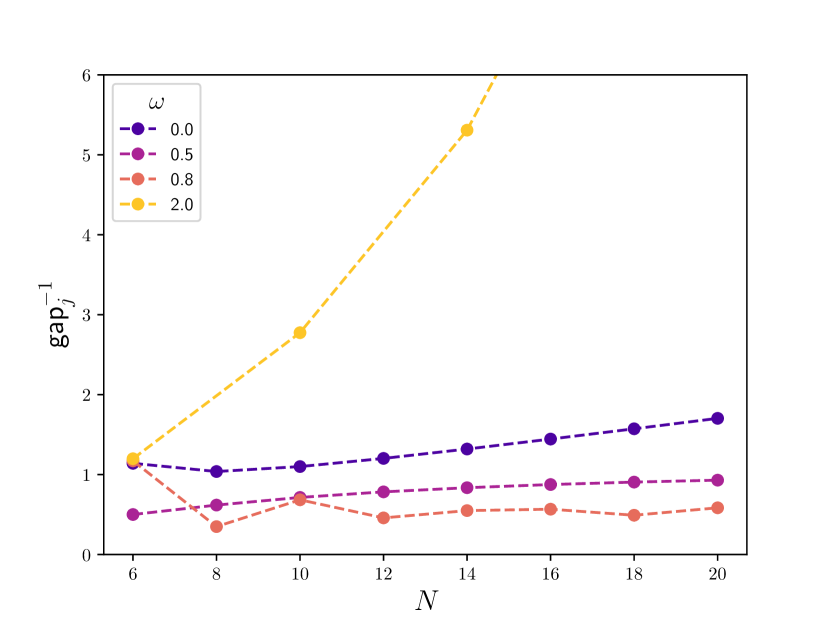
Figure 3: Magnitude of the gap above the blind subspace (gap_j) as a function of the system size $N$ for different values of $\omega$. Dotted lines have been added between data points to guide the eyes.

In Fig. 3, the inverse gap above the blind subspace is plotted for representative points in the qubit VBS subspace ($\omega=0.8$), in the ’Heisenberg’ subspace ($\omega=0$), and in the qutrit VBS subspace ($\omega=2$). The Majumdar-Gosh point ($\omega=0.5$) is also plotted. As can be seen form this figure, the gaps for values of $\omega$ in the ’Heisenberg’ and qubit VBS regions are relatively constant, with some indications of slowly decreasing gaps as system size is scaled up. However, in the qutrit-region $\omega\geq 1.5$ the gap closes rapidly, corresponding to the disappearance of the protected subspace. Note that the qutrit blind subspace is only observed for $N\equiv 2\,(\mathrm{mod}\,4)$, meaning the observed vanishing gap is consistent with an expectation that $N\equiv 2\,(\mathrm{mod}\,4)$ and $N\equiv 0\,(\mathrm{mod}\,4)$ should behave equivalently in the thermodynamic limit.

V.2.2 Contributions from the bulk of the spectrum

In the main text, it was conjectured that for low enough temperatures, the following holds as the number of quits is increased:

$$\mathcal{K}(N,\beta,\omega):=\sum_{k>j+1}e^{-\beta(e_{k}-e_{j+1})/2}|\langle e_{k}|S_{a}|e_{j}\rangle|\sim O(1)\;,$$

where $e_{k}$ are the eigenenergies of the system numbered in increasing order, and $j$ is the index of the high-energy state of the blind qubit subspace. Here, we provide numerical evidence to support this claim, and explore what constitutes sufficiently low temperatures.

First, note that

$$\mathcal{K}(N,\beta,\omega)\leq\mathcal{C}(N,\beta,\omega):=\sum_{k>j+1}e^{-\beta(e_{k}-e_{j+1})/2}\;.$$

If the degeneracy for the energy level that the $(j+1)$th state belongs to is $D(N,\omega)$, the sum takes the form

$$\mathcal{C}(N,\beta,\omega)=D(N,\omega)+\sum_{k>(j+D)}e^{-\beta(e_{k}-e_{j+1})/2}$$ (27)

where now the energies in the exponent of the sum are all positive by definition. Thus, in the limit of $\beta\rightarrow\infty$, $\mathcal{C}(N,\beta,\omega)$ and $D(N,\omega)$ coincide. Arguing that $\mathcal{C}\sim O(1)$ therefore boils down to arguing that a) $D(N,\omega)\sim O(1)$, i.e., that the degeneracies of the low-energy spectrum does not grow with system size, and b) the temperature scale where $\mathcal{C}\simeq D$ remains constant, or at the very least only shrinks at a relatively slow rate. To get an intuition for both of these questions, the evolution of $\mathcal{C}$ towards $D$ as $\beta$ is increased is depicted in Fig. 4 for $\omega=0$, i.e., in the Heisenberg phase.

Figure 4: Evaluation of $\mathcal{C}(N,\beta,\omega)$ as a function of $\beta$ for $\omega=0$ and various system sizes.

As can be seen from this figure, the limit of $\mathcal{C}$ as beta is increased is the same as $N$ is increased, indicating that the degeneracy $D$ does not depend on the system size for even-size systems. This was additionally numerically verified up to a system size of $N=22$ using the Lanczos algorithm for finding top eigenvalues. A similar independence of $D$ to system size was observed across a range of $\omega$ in the relevant regimes, including in the qutrit-regime $\omega\gtrsim 1.5$ for systems of the size where this subspace is present, i.e., systems where $N\equiv 2\,(\mathrm{mod}\,4)$.

The results above provide support to the first of the two claims, namely that the degeneracies of the low-energy spectrum is independent of system size, meaning the low-temperature limit of $\mathcal{C}(N,\beta,\omega)$ is also indpendent of system size. However, as can be seen in Fig. 4, the rate at which the asymptotic value is reached does depend on the system size, with larger systems typically displaying a slower decay. One way to quantify this slowdown is to investigate how large a value of $\beta$ is required to achieve a certain value of $\mathcal{K}$,

$$\beta^{*}(N,\omega,K)=\inf\{\beta:Ne^{-\beta{\rm gap_{j}}/2}\mathcal{K}(N,\beta,\omega)\leq K\}\;.$$ (28)

Figure 5: Numerical calculations of $\beta^{*}(N,\omega,K)$, the value of $\beta$ required to achieve a given suppression $K$ in Eqn. (10). The corresponding values for the inverse gap has been added for reference, and dotted lines added to guide the eyes.

This quantity is depicted on Fig. 5 for $\omega=-0.1$ and $\omega=0.6$. The values of $\omega$ were chose to lie deep in the two metastable phases, while avoiding the special points ($\omega=0$ and $\omega=0.5$). While it is difficult to make any strong claims based on the figure, the value of $\beta$ necessary to reach a given protection does appear to increase slowly beyond $N\approx 10$. A similar behavior is seen for other choices of $\omega$. The exact way that $\beta^{*}$ evolves as $N$ grows depends on $\omega$ and $K$, but often follows the pattern observed in Fig. 5, where stricter (lower) values of $K$ has a positive curvature, while more lenient (higher) values of $K$ has a negative curvature. One exception is near $\omega\simeq 0.8$, where oscillatory finite-size effects are observed, similarly to the behaviour of the gaps in Fig. 3.

In conclusion, numerics suggest that if $\beta\geq\beta^{*}$ for a $\beta^{*}$ that increases sub-linearly with system size, the scaling $\mathcal{C}=O(1)$ is achieved, and all of the decoherence-inducing contributions are therefore bounded by $O(e^{-\beta\mathrm{gap}_{j}/2})$. Since the inverse gap also scales approximately linearly (see Fig. 3), both of these effects enforce an approximately linearly increasing $\beta$ with system size.

V.2.3 Phase transition points as the system scales up

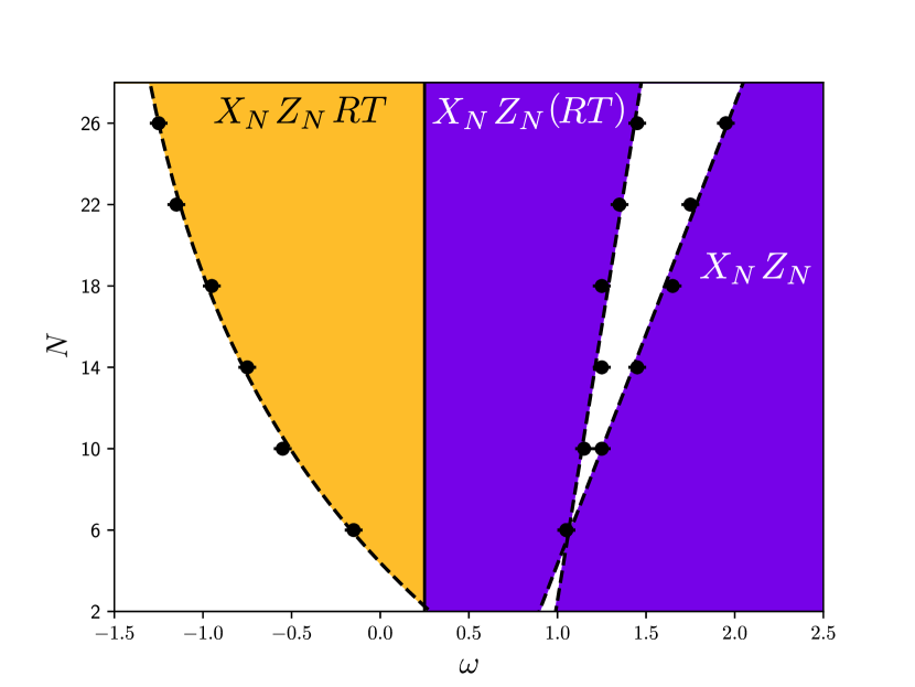
Figure 6: Location of the transitions between metastable phases. From left to right, the second region hosts a protected qubit, while the fourth hosts a protected qutrit. Fits are either linear or exponential in the system size, depending on the observed behaviour. For the exponential fit, a limit of $\omega^{*}_{L}\simeq-1.647$ is predicted, with the characteristic scale of $k^{-1}\simeq 15$ in the exponential decay $\omega(N)=\omega^{*}_{L}+(\omega_{L}^{(0)}-\omega^{*}_{L})e^{-kN}$.

A compelling feature of the results presented here, is that the transitions into and out of metastable subspaces do not appear to coincide with the ground state phase diagram for finite $N$. To test whether this feature survives as the chain length grows, we plot the (approximate) locations of the transitions points in Fig. 6. The numerics suggest that the transitions to the qubit and qutrit metastable subspaces grow linearly with $N$, strongly suggesting that the qubit metastable subspace will cover the whole phase in the thermodynamic limit. The ’Heisenberg’ subspace is also moving left as the system size increases, but it is difficult to know whether it will continue expanding as the system size grows further.

If the two phases extend out to infinity, this would suggest that the metastability ’phase diagram’ coincides with the ground state phase diagram for the $J_{-}J_{2}$ model. In parallel experiments, that are not reported here, we found that this is clearly not the case for the XXZ Heisenberg model, which undergoes a metastable transition at zero ZZ field strength, which does not coincide with the ground state phase transition of the model.

Finally, in view of the observation above, that the critical temperature $\beta^{*}$ above which there is exponential survival of the blind subspace grows with system size, the effects that we report are most pronounced for finite chains.