RISE-iEEG: Robust to Inter-Subject Electrodes Implantation Variability iEEG Classifier

Abstract

Objective: Utilization of intracranial electroencephalography (iEEG) is rapidly increasing for clinical and brain-computer interface applications. iEEG facilitates the recording of neural activity with high spatial and temporal resolution, making it a desirable neuroimaging modality for studying neural dynamics. Despite its benefits, iEEG faces challenges such as inter-subject variability in electrode implantation, which makes the development of unified neural decoder models across different patients difficult. Approach: In this research, we introduce a novel decoder model that is robust to inter-subject electrode implantation variability. We call this model RISE-iEEG, which stands for Robust Inter-Subject Electrode Implantation Variability iEEG Classifier. RISE-iEEG employs a deep neural network structure preceded by a patient-specific projection network. The projection network maps the neural data of individual patients onto a common low-dimensional space, compensating for the implantation variability. In other words, we developed an iEEG decoder model that can be applied across multiple patients’ data without requiring the coordinates of electrode for each patient. Main results: The performance of RISE-iEEG across multiple datasets, including the Audio-Visual dataset, Music Reconstruction dataset, and Upper-Limb Movement dataset, surpasses that of state-of-the-art iEEG decoder models such as HTNet and EEGNet. Our analysis shows that the performance of RISE-iEEG is 10% higher than that of HTNet and EEGNet in terms of F1 score, with an average F1 score of 83%, which is the highest result among the evaluation methods defined. Furthermore, the analysis of projection network weights in the Music Reconstruction dataset across patients suggests that the Superior Temporal lobe serves as the primary encoding neural node. This finding aligns with the auditory processing physiology. Significance: The projection network effectively addresses the variability in electrode implantation, significantly improving classification accuracy. Therefore, we believe the proposed model will find broad applications in neural decoding tasks, offering better decoding accuracy without sacrificing interpretability and generalization.

• August 2024

Keywords: Intracranial Electroencephalography (iEEG), Neural Decoder Model, iEEG Decoder, Deep Neural Network

1 Introduction

Researchers use numerous techniques to record brain activity, thereby enhancing their understanding of brain functions and aiding in the diagnosis and treatment of diverse neurological conditions [1]. Among these recording techniques, iEEG provides a balanced measure of temporal and spatial resolutions. Initially employed for patients with epilepsy to detect seizures, its recent applications have expanded with the advancements in analog design and neural interface technology. Like other neuroimaging techniques, iEEG has its own limitations. Given its invasive nature, electrode implantation must be justified based on patient health benefits and ethical considerations, limiting our access to common implantation coordinates across participants in neuroscience experiments. Simply, with iEEG, neural data recorded across patients have inconsistent and non-overlapping brain coverage [2]. To effectively leverage the iEEG dataset, we need to develop analytical tools that can address the variability in electrode placement and configuration.

Beyond utilizing iEEG data for seizure prediction or localization [3], [4], [5], [6], iEEG data has been vastly used for neural decoding and interface applications. These applications encompass, but are not limited to, decoding visual stimuli [7], [8], [9], audio-visual stimuli [10], speech silently conveyed by participants [11], and motor imagery [12]. As such, many analytical solutions have been developed to analyze iEEG data and map them to the stimuli space. These include traditional techniques such as SVM classifier [9], Bayesian linear discriminant analysis [13], K-Nearest Neighbor [14], and more recent techniques such as Bayesian Time-Series classifier [7]. Recent deep models are becoming a standard pipeline for decoding tasks as they provide an end-to-end modeling pipeline eliminating multiple pre-processing and feature extraction steps needed in the traditional decoding approaches [15].

Among deep modeling solutions, a notable model is EEGNet [16], which has been successfully applied to different datasets, including the Motor imagery dataset [17], and EEG-ImageNet dataset [18]. Deep learning models often need large amounts of data, so the challenge of limited datasets makes their utility for iEEG data somewhat difficult. Moreover, variations in electrode placement complicate the development of a unified model applicable across multiple patients. A solution to address this challenge was introduced in [19] with the design of the HTNet model. Its objective is to standardize electrode positioning by mapping them to a common space, similar to a standard EEG cap. This method facilitates the training of models on data from various patients by overcoming the variation of electrode location. However, this approach requires precise electrode positioning in the Montreal Neurological Institute (MNI) space [20]. The process of finding MNI coordinates of electrodes requires co-registering preoperative MRI and postoperative CT scans, which is time-consuming and prone to errors. As a result, MNI electrode location data are not present in many publicly available iEEG datasets, making it impossible to map electrode positions to a common space. Additionally, the mapping approach in this model is based on the distances of electrodes from common brain regions. However, this might not be an appropriate approach for the mapping process, as previous research has demonstrated that functional connections between brain areas do not rely on their physical distance [21]. Given these challenges, we think that developing new techniques to address electrode implantation variability holds significant value in expanding the utility of iEEG data in both clinical and basic neuroscience domains.

In this research, we introduce the RISE-iEEG model, designed to address the challenges of electrode implantation variability and to overcome the limitations of the approach used in the HTNet model. The RISE-iEEG model is built using projection and discriminative networks. The projection network maps the iEEG data of individual patients onto a common space using linear mappings, without requiring the MNI coordinates of electrodes. The weights of the projection network in the RISE-iEEG model are tuned during the training step. The discriminative network, shared across all patients, has an architecture similar to EEGNet, employing a temporal and spatial convolutional neural network to extract useful features from the data for classification. In this study, we discuss the RISE-iEEG architecture, its training process, and model assessment using various datasets. We also explore methods to interpret the trained model, aiming to investigate neural encoding mechanisms. We believe that post-training and performance analyses will validate the model architecture and demonstrate its utility in building a scalable and generalizable decoder model for iEEG and potentially EEG datasets.

The subsequent sections of this paper are organized as follows. In section 2, we provide a detailed description of the architecture and training process of the RISE-iEEG model. In this section, we also define the various cross-validation paradigms used to assess the model’s performance. In section 3, we introduce the publicly available iEEG datasets used in this research. We then present the decoding results of RISE-iEEG and compare them with those from other state-of-the-art decoders, such as HTNet and EEGNet. Additionally, we analyze the trained weights of the projection network and elaborate on their connection to potential neural encoding mechanisms. In Section 4, we discuss the advantages and limitations of our proposed model compared to other decoder models. The conclusions are presented in Section 5.

2 Material and Methods

2.1 RISE-iEEG Model Architecture

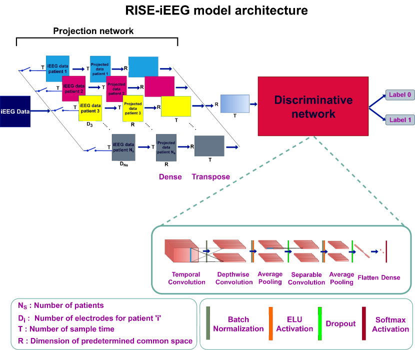
Figure 1: The RISE-iEEG model comprises two main network: projection network and discriminative network. The projection network has a specified dense layer for each patient and functions as a linear transformation to map electrode positions onto a common space. The discriminative network has an architecture similar to EEGNet [16] and extracts useful features from the projected data using temporal and spatial convolutional neural networks.

The RISE-iEEG is a cascade deep neural network comprising a patient-specific projection network followed by a discriminative deep neural network. The patient-specific projection layer features a linear transformation to map the input dimension to a (potentially lower-dimensional) common space, aiming to address variability in electrode placement across patients. The linear transformation in this layer ensures that subsequent layers in the network are fed with a consistent representation of the iEEG data from various patients, which enhances the network’s ability to extract features that are robust across different patients. By applying this mapping, we expect the model to improve its generalization capabilities and accuracy in classifying neural patterns, regardless of variations in electrode placement across patients. The data for each patient is structured as a three-dimensional matrix with dimensions $T\times D_{i}\times Ne$, where $T$ is the number of time samples, $D_{i}$ is the number of electrodes for patient $i$, and $Ne$ is the number of events. While $T$ and $Ne$ are consistent across patients, $D_{i}$ varies. In this mapping, for the $i$-th patient with $D_{i}$ electrodes implanted, the input dimension $D_{i}$ is mapped to a common space with dimension $R$, which is shared across patients. The structure of the RISE-iEEG model is illustrated in Fig.1.

For the linear transformation, the projection network includes dense layers corresponding to the number of patients, mapping each patient’s data onto a common space. Each dense layer is designed so that its input nodes align with the number of electrodes for the respective patient ($D_{i}$), and its output nodes correspond to the predetermined dimension of the common space ($R$). As shown in Fig.1, in the projection network, a ’switch’ mechanism is placed before each dense layer. This switch directs the iEEG data of each patient to their respective dense layer through separate pathways.

The discriminative network is a non-linear mapping from the common space time-series data to class label and is shared across all patients’ data. This network has the same architecture as the EEGNet [16] model, and consists of the temporal and spatial convolutional neural networks. The combination of these convolutional layers leads to effectively processing the data in both temporal and spatial domains.

2.2 Cross-Validation Paradigms

Given that we were dealing with data from multiple patients and had a patient-specific layer in RISE-iEEG, we defined different cross-validation paradigms to assess the model’s performance. The way the data were split for train, test, and validation sets will affect how we can train the network. We defined two settings that align with our objective to assess classifier performance across multiple patients and to probe its generalization. These settings were called ’same patient’ and ’unseen patient’. We first discuss the different cross-validation pipelines before discussing the model training.

In the ’same patient’ setting, the training and test sets include data from the same patients. We employed pseudo-random selections (folds) to evaluate the model’s performance. Within each fold, the data from each patient were divided into training, validation, and test sets. After training the model with the balanced training set, we evaluated its performance using the test set.

In the ’unseen patient’ setting, the training and test sets include data from different patients. As explained in Section 2.1, the projection network consists of separate dense layers tailored to each patient. The weights and structure of these dense layers vary among patients due to differences in the positions and numbers of electrodes used for each patient. Consequently, the projection network must be trained on data from new patients not included in the training set. So, in this setting, the model is trained in two steps. In the first step, the model is trained with data from all minus one patient. In the second step, the projection network is solely trained with a portion of the test patient’s data, while the layers of the discriminative network remain frozen. To evaluate the model’s performance, we employed leave-one-out cross-validation (LOOCV), consisting of $N_{p}$ folds, with each fold representing one patient. In each fold, the data of one patient was in the test set, while the data from other patients were in the training and validation sets.

2.3 Model Training

For model training, we used stochastic batch training [22]. In each iteration, we randomly select a set of samples that come from multiple patients, instead of just one. During the feed-forward step, each sample is fed into the model, activating the corresponding patient switch. In the backpropagation step, we calculate the mean loss function for all the samples in the batch. Subsequently, the discriminative network and the dense layer of the selected patients are updated, while the dense layers of the other patient remain frozen, as they do not have input data. Finally, in each epoch, where the model is fed with all sample data from all patients, the discriminative network is updated with data from all patients, and each patient-specific dense layer is updated with data from its respective patients.

In the process of model training, we implemented early stopping to prevent overfitting by monitoring the validation accuracy. The training was conducted using batch gradient descent with a batch size of 16 and the Adam optimizer. To regularize the model, we employed the L2 regularization method [23] in the dense layers of the projection part to prevent overfitting the model when training with small sample sizes.

For our model training, we utilized TensorFlow 2.2 as our deep learning framework. The training was conducted on a Windows system equipped with two GTX 1080 GPUs and 32GB of RAM. These resources provided the necessary computational power to efficiently handle the data and perform the required calculations.

3 Results

3.1 Dataset

In this research, we evaluated the performance of RISE-iEEG in three datasets, i.e., Audio Visual dataset [24], Music Reconstruction dataset [25], and Upper-Limb Movement dataset [19]. These diverse tasks enable a comprehensive assessment of the RISE-iEEG model across different domains, ensuring its robustness and versatility. The datasets used in this study are all publicly available and follow the recommended IRB protocols of their respective institutions.

• Audio Visual dataset: This dataset was introduced in [24], which comprises iEEG data collected from 51 patients while they watched a short film in French. The number and position of implanted electrodes varies among patients. The short film has a duration of 6 minutes and 30 seconds, featuring alternating segments of actors’ speech and music, each lasting 30 seconds. The dataset also includes annotations for the onset and offset of sentences spoken by the actors, some of which were in question form. It is worth mentioning that for this dataset, neither the MNI coordinates of the implanted electrodes nor the postoperative CT scans were available. Based on this dataset, we define two classification tasks: ’Speech vs. Music’ and ’Question vs. Non-Question Sentences’.

  For the task ’Speech vs. Music’, we divide the data into 2-second events, resulting in 105 ’Music’ events and 90 ’Speech’ events for each patient. For the task ’Question vs. Non-Question Sentences’, we segmented the data into 3-second events, spanning from 0.5 seconds before the onset of the sentence to 2.5 seconds after. Consequently, we obtained 67 ’Non-Question’ events and 15 ’Question’ events for each patient. The duration of each time window was empirically chosen based on our model’s performance.

• Music Reconstruction dataset: This dataset, introduced in [25], consists of iEEG data recorded from 29 neurosurgical patients while they listened to rock music. The positions of electrodes were determined based on clinical considerations and were placed either in the right or left hemisphere (11 on the right, 18 on the left). Electrode positions noticeably vary among patients. In this dataset, the MNI coordinates of the electrodes were provided.

  The music played for patients included vocals for a total of 32 seconds and instrumental music without words for 2 minutes and 26 seconds. We defined the classification task ’Singing vs. Music’ for this dataset. For this task, we divided the data into 2-second events, resulting in 16 ’Singing’ events and 73 ’Music’ events for each patient. Similarly, the duration of the time window for this dataset was also selected empirically.

• Upper-Limb Movement dataset: This dataset, presented in [19], includes iEEG data captured from 12 patients during their clinical epilepsy monitoring. Moreover, a video was simultaneously recorded to identify instances when patients moved their upper limbs. Each patient’s electrodes were located in one hemisphere (5 on the right, 7 on the left), and the positions of the electrodes varied among patients. For this dataset like the Audio Visual dataset, the MNI coordinates of the electrodes and postoperative CT scans were not provided.

  In this dataset, the classification task ’Move vs. Rest’ is defined based on upper-limb movement. Data were segmented into 2-second time windows centered around each ’Move’ and ’Rest’ event. As a result, there are at least 150 ’Move’ events and 150 ’Rest’ events for each patient.

3.2 Competing Models

We compared the performance of RISE-iEEG with other multi-patient decoders such as HTNet, EEGNet, Random Forest, and Minimum Distance, as implemented in [19]. Unlike RISE-iEEG, these decoders require the MNI coordinates of electrodes for individual patients. Here, we briefly discuss the attributes and architectures of these models.

1. EEGNet: EEGNet [16] is a convolutional neural network consisting of several 2-D convolutional layers designed to extract spatial and temporal patterns from neurological data. In [19], a projection block is added after the temporal convolution in the EEGNet architecture to map the electrode data onto regions of interest (ROIs), thereby facilitating the decoding of data from multiple patients. This projection block comprises patient-specific projection matrices, and it is implemented as a matrix multiplication layer. These matrices are generated by computing the radial basis function (RBF) kernel distances between each electrode and each brain region. Thus, EEGNet requires the MNI coordinates of electrodes to construct patient-specific projection matrices.

2. HTNet: HTNet shares a similar architecture to EEGNet. However, in HTNet, a Hilbert transform layer is added right after the initial temporal convolution layer. This extra layer enables the network to extract relevant spectral power features from the data [19].

3. Random Forest: In this model, the neural data from each patient are initially projected onto ROIs using the projection block designed in the modified EEGNet architecture. This projection process enables the application of the Random Forest classifier to the neural data of all patients [26].

4. Minimum Distance: In this model, similar to the Random Forest classifier, the data of each patient is first projected onto ROIs. Subsequently, the Minimum Distance classifier utilizes Riemannian mean and distance values to classify the projected data of all patients [27].

These models are widely used in the analysis of EEG/iEEG data and have demonstrated high classification accuracy [19].

3.3 RISE-iEEG Performance in ’same patient’ Setting

In this study, we utilized 10 pseudo-random selections (folds) to assess the performance of the RISE-iEEG model. Within each fold, the training, validation, and test sets comprised 64%, 16%, and 20% of the data from each patient, respectively. Initially, the model was trained as described in section 2.3.

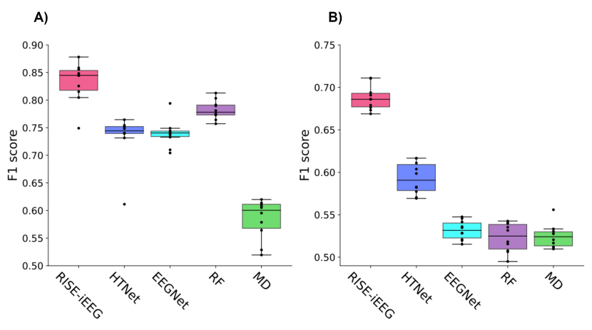
Figure 2: Performance comparison of the RISE-iEEG model (pink) with HTNet (blue), EEGNet (light blue), Random Forest (RF, purple), and Minimum Distance (MD, green) decoders, presented separately for each model in the ’same patient’ setting across two tasks: (A) the ’Singing vs. Music’ task and (B) the ’Move vs. Rest’ task. Each point represents the mean F1 score of each fold across patients.

We evaluated the model’s performance on each patient’s test set data using the F1 score metric, as it provides a balanced measure of precision and recall. The performance of the RISE-iEEG model was assessed across the four classification tasks, and the results are presented in Table 1. As shown in the table, the RISE-iEEG model demonstrates acceptable performance in classifying tasks across various domains. We cannot apply other state-of-the-art decoders, such as HTNet and EEGNet, to the Audio Visual dataset because, as explained in section 3.1, this dataset does not provide MNI coordinates of the electrodes. However, we applied RISE-iEEG to this dataset to demonstrate that our model is applicable to various datasets with diverse tasks.

We compared the performance of the RISE-iEEG model with state-of-the-art decoders, as explained in section 3.2. Given that only the Music Reconstruction dataset contains MNI coordinates for the electrodes and the Upper-Limb Movement dataset provides the necessary projection matrices, our comparison was limited to these two datasets. It is worth mentioning, that we trained and tested all these comparison models exactly similar to that of the RISE-iEEG model. The results of comparing the performance of these models are illustrated in Fig.2.

Table 1: RISE-iEEG performance in the ’same patient’ setting for each task

Dataset	Task	F1 score(mean±SD)
Audio Visual dataset [24]	Speech vs. Music	0.79 ± 0.02
Audio Visual dataset [24]	Question vs. Non-Question Sentences	0.69 ± 0.01
Music Reconstruction dataset [25]	Singing vs. Music	0.83 ± 0.03
Upper-Limb Movement dataset [19]	Move vs. Rest	0.68 ± 0.01

The results in Fig.2 demonstrate that the RISE-iEEG model outperformed other state-of-the-art models in both tasks. For the ’Singing vs. Music’ classification, RISE-iEEG achieves a test F1 score of 0.83 ± 0.03, outperforming HTNet (0.73 ± 0.04), EEGNet (0.74 ± 0.02), Random Forest (0.78 ± 0.01), and Minimum Distance (0.58 ± 0.03). In the ’Move vs. Rest’ classification, RISE-iEEG attains a test F1 score of 0.69 ± 0.01, exceeding HTNet (0.59 ± 0.01), EEGNet (0.53 ± 0.01), Random Forest (0.52 ± 0.01), and Minimum Distance (0.52 ± 0.01). Moreover, RISE-iEEG exhibits a lower variance in classification F1 scores across folds compared to other decoders, indicating greater consistency in its performance. This consistency suggests that RISE-iEEG is more robust and reliable.

3.4 RISE-iEEG performance in ‘unseen patient’ setting

We evaluated the model’s performance using leave-one-out cross-validation (LOOCV). For each fold, one patient’s data was included in the test set, and the discriminative network was trained with the data from the remaining $N_{p}-1$ patients. Subsequently, we performed 3 pseudo-random selections (inner folds) on the data of the test patient. In each inner fold, we fine-tuned the projection network using a portion of the test patient’s data and assessed the model’s performance using the remaining data.

We evaluated the performance of the RISE-iEEG model against state-of-the-art decoders in the ’unseen patient’ setting. For the ’Singing vs. Music’ classification task, RISE-iEEG achieved a test F1 score of 0.80 ± 0.05, outperforming HTNet (0.60 ± 0.12), EEGNet (0.67 ± 0.11), Random Forest (0.71 ± 0.07), and Minimum Distance (0.49 ± 0.23). In the ’Move vs. Rest’ classification, RISE-iEEG attained a test F1 score of 0.74 ± 0.07, surpassing HTNet (0.62 ± 0.07), EEGNet (0.59 ± 0.06), Random Forest (0.59 ± 0.06), and Minimum Distance (0.55 ± 0.05). The results of these comparisons for each patient individually are illustrated in Fig. 3 (A, B). As shown in this figure, RISE-iEEG notably outperformed other models in classifying data from 23 out of 29 patients in the ’Singing vs. Music’ task and from 11 out of 12 patients in the ’Move vs. Rest’ task.

To determine the optimal data ratio for fine-tuning the projection network, we explored how model performance changes with different ratios of data split between the fine-tuning and test sets. As shown in Fig.3 (C, D), for both tasks, the model’s performance improves as the size of the fine-tuning set increases. However, starting from a ratio of 60%, the model’s performance becomes almost constant, and at a ratio of 90%, the model’s performance decreases due to overfitting caused by the large size of the fine-tuning set.

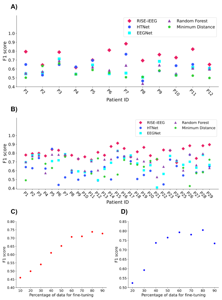
Figure 3: (A, B) Performance comparison of the RISE-iEEG model (pink) with HTNet (blue), EEGNet (light blue), Random Forest (purple), and Minimum Distance (green) decoders, shown separately for each patient in the ’unseen patient’ setting across two tasks: (A) the ’Move vs. Rest’ task and (B) the ’Singing vs. Music’ task. (C, D) Effect of fine-tuning data ratio on model performance for two tasks: (C) the ’Move vs. Rest’ task and (D) the ’Singing vs. Music’ task.

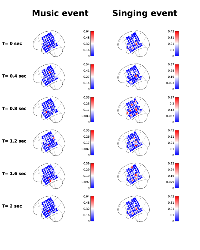
Figure 4: Temporal variation in the mean IG across events for a single patient, highlighting the importance of each electrode at different time points (0, 0.4, 0.8, 1.2, 1.6, and 2 seconds) after stimulus onset. The left column represents the IG maps for the ’Music event’, and the right column for the ’Singing event’. The color scale represents the magnitude of IG, with red representing higher importance and blue representing lower importance.

3.5 Interpretation of Trained RISE-iEEG Model

We aim to determine how stimuli are encoded in the neural activity of different nodes during a specific task. To address this, we employed the Integrated Gradient method (IG) [28], which is an interpretability technique for deep neural networks. In this method, the gradient of the model’s prediction output with respect to its input data is computed to identify which spatio-temporal inputs have the strongest influence on the model’s output.

In this process, accessing the MNI coordinates of the electrodes is essential for identifying the significant lobe for each patient. Consequently, our analysis to interpret the trained weights of the RISE-iEEG model was limited to the Music Reconstruction dataset for the ’Singing vs. Music’ task.

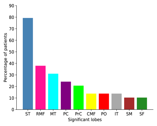
Figure 5: The distribution of significant brain lobes across patients. The significant lobes and their respective colors are as follows: Superior Temporal (ST - blue), Rostral Middle Frontal (RMF - pink), Middle Temporal (MT - cyan), Postcentral (PC - purple), Precentral (PrC - lime), Caudal Middle Frontal (CMF - yellow), Pars Opercularis (PO - red), Inferior Temporal (IT - gray), SupraMarginal (SM - brown), and Superior Frontal (SF - dark green).

To explore the encoding mechanism, we performed various analyses using the IG method. We first computed IG for all events of each patient, indicating the importance of data from each electrode at each time sample. The temporal variation in the mean IG across events for a single patient is depicted in Fig.4. This figure reflects the significance of each electrode at 400 msec intervals. As shown in this figure, the temporal lobe consistently exhibits relatively high weights throughout all time intervals following stimulation. This suggests that this lobe has a greater contribution to label prediction in the ’Singing vs. Music’ task, indicating that it carries more relevant data for this task. This finding aligns with our expectations, as the task of the Music reconstruction dataset was related to auditory processing for classifying ’Music’ vs. ’Singing,’ and the temporal lobe is the first area responsible for interpreting information in the form of sounds from the ears [29].

Moreover, we summed the computed IG for each event along the time axis to identify the brain lobe with the highest weight, designating it as the significant lobe for each event. For each patient, we then arranged these significant lobes from all events based on their reproducibility. We explored the top three lobes with the highest reproducibility for each patient to provide a more comprehensive analysis.

Fig.5 illustrates the percentage of patients for which each lobe ranks among the top three most significant lobes. As shown, the Superior Temporal (ST) lobe is one of the three significant lobes in 80% of patients, suggesting that this lobe is particularly important for this task and contains highly informative data for classification. This finding aligns with previous ECoG research [25], [11], which emphasizes the crucial role of the Superior Temporal lobe in music perception and interpretation.

The IG method evaluates the importance of data from each brain region across all network layers. In contrast, we can specifically analyze the projection network by examining the weights of each patient-specific dense layer within this network. This analysis allows us to determine the contribution of each brain region in the common space. As presented in Tab.2, our findings indicate that, for most patients, the Superior Temporal Lobe exhibits the highest mapping weight among all regions, consistent with the results obtained using the IG method.

Table 2: The lobe brain with the highest weight in patient-specific projection layer for each patient

patient	Lobe	patient	Lobe	patient	Lobe
1	Superior Temporal	11	Superior frontal	21	Rostral middle frontal
2	Superior Temporal	12	Precentral	22	Superior Temporal
3	Superior Temporal	13	Parsorbitalis	23	Inferior temporal
4	Superior Temporal	14	Superior Temporal	24	Superior Temporal
5	Superior Temporal	15	Superior Temporal	25	Superior Temporal
6	Superior Temporal	16	Precentral	26	Superior Temporal
7	Superior Temporal	17	Superior Temporal	27	Superior Temporal
8	Superior Temporal	18	Superior Temporal	28	Supra marginal
9	Precentral	19	Superior Temporal	29	Superior Temporal
10	Superior Temporal	20	Superior Temporal

3.6 Role of Projection Network

The performance results indicate the importance of the projection network in the RISE-iEEG model. To gain a clearer understanding of its role, we have carried out several analyses and assessments to elucidate its contribution to the model and its impact on achieving a more robust outcome.

A key modeling question concerns the sensitivity of the RISE-iEEG model, particularly the projection network, to the order of the electrodes in the input data. Based on the results in section 3.5, RISE-iEEG is not sensitive to the order of channels and can effectively identify the informative channels in the input data to extract meaningful information. For instance, patients 1 and 2 both have electrodes in the Superior Temporal lobe, but the positions of these electrodes differ between their datasets. Despite this variation, the RISE-iEEG successfully identified the Superior Temporal lobe as the significant lobe for both patients.

To study the role of the projection network in spatial mapping across neural nodes, we evaluated the classification accuracy of RISE-iEEG, HTNet, and EEGNet, both with and without the spatial convolution layer (Depthwise Convolution layer) in the discriminative network. Without the spatial convolution layer, the classification accuracy dropped in all models; however, the percentage of accuracy reduction in RISE-iEEG was greater than in the other models. It is worth mentioning that even without the spatial convolution layer, RISE-iEEG outperformed than HTNet and EEGNet models. This indicates that the classification accuracy of RISE-iEEG is significantly influenced by the spatial convolution layer. This means that the projection network in RISE-iEEG effectively maps electrode positions, allowing the spatial convolution layer to extract more useful spatial features resulting in better performance compared to other models.

As outlined in section 3.5, we found that, for the ’Singing vs. Music’ task, the Superior Temporal lobe and the Rostral Middle Frontal lobe are core nodes of neural activity, providing the most informative data. To further validate this finding, we excluded data from the Superior Temporal lobe across all patient’s datasets and assessed the performance of the RISE-iEEG model again. This led to about a 10% drop in the model’s performance, confirming what we inferred using IG analysis about the role of the Superior Temporal lobe. Furthermore, the application of IG to this modified model revealed that the Rostral middle frontal lobe contains the most relevant data in the absence of the Superior Temporal lobe’s data. These observations suggest that, when data from the Superior Temporal lobe is unavailable, the model primarily relies on data from the second core nodes, i.e., the Rostral Middle Frontal lobe for prediction, indicating the robustness of our model.

4 Discussion

In this work, we demonstrated that the classification accuracy of CNN-based neural decoder models can be significantly enhanced by designing a patient-specific projection network. This proposed solution not only improves classification accuracy but also eliminates the need for MNI coordinates of implanted electrodes. The projection network maps data from various electrodes onto a common space using adaptive weights determined during the training phase, thereby simplifying its application across different iEEG datasets. The discriminative network of RISE-iEEG employs a convolutional neural network architecture, similar to EEGNet, to effectively extract temporal and spatial features from neural data.

Our evaluation of the RISE-iEEG model in ’same patient’ and ’unseen patient’ settings in three different datasets demonstrated better performance compared to state-of-the-art decoder models such as HTNet, EEGNet, Random Forest, and Minimum Distance. This consistent outperformance highlights the model’s robustness and capability to compensate for electrode implantation variability across patients. Furthermore, using the IG method, we demonstrated that the ’Singing vs. Music’ task is encoded in the Superior Temporal lobe of the brain for most patients.

We demonstrated that the embedded projection network in the RISE-iEEG model efficiently compensates for the lack of MNI coordinates of electrodes, which is necessary information in the development of other state-of-the-art decoders, such as HTNet. This feature allows us to apply the RISE-iEEG model to many more iEEG datasets, as MNI coordinates are often not available in these datasets.

The projection network in the RISE-iEEG model has trainable weights. This feature allows the model to optimize the mapping process such that the discriminative network can extract more informative features from neural data. This ultimately leads to higher classification accuracy for the model. In contrast, the weights of the projection matrices in state-of-the-art decoders are fixed and determined using a radial basis function kernel based on the physical distance of each electrode to each region of interest (ROI). Since functional connectivity between brain areas is independent of their physical distance [21], this approach does not accurately reflect the reality of brain function, leading to lower classification accuracy.

RISE-iEEG eliminates the need for pre-computation before the training phase when dealing with decoding data from multiple patients. In contrast, HTNet requires the generation of projection matrices before model training. This process involves selecting hyperparameters, such as the appropriate ROIs and the sigma value for the radial basis function kernel. As a result, RISE-iEEG offers a more simplified and flexible approach to decoding and reduces the time required for model preparation compared to HTNet.

While RISE-iEEEG attains a higher prediction accuracy, it still has its limitations. Our model faces two significant limitations. First, the RISE-iEEG model requires fine-tuning of the projection network with a portion of data from a new patient not present in the training set. Second, the number of parameters in the RISE-iEEG model is higher than in other decoders, such as HTNet, due to the trainable weights of the projection network. This can create challenges when applying the RISE-iEEG model to datasets with limited sample sizes. However, our observations based on the results suggest that using the L2 regularization method in the RISE-iEEG model enables it to perform similarly to HTNet and EEGNet with the same amount of data. In other words, the RISE-iEEG does not require a larger dataset to achieve comparable performance to these models.

In conclusion, we believe that the RISE-iEEG model presents a robust and interpretable architecture, capable of making significant advancements in the field of generalized neural decoder design. By addressing key limitations of existing techniques, it offers a robust and adaptive solution for decoding neural activity across diverse patient data. The promising results from our evaluations emphasize the model’s potential for significant contributions to neuroscience research.

5 Conclusion

In this study, we introduced the RISE-iEEG model, a generalizable neural decoder that is applicable to iEEG data collected from various experiments. Our proposed model features a patient-specific projection network followed by a discriminative deep neural network. The projection network maps each patient’s data into a common low-dimensional space, ensuring that the discriminative network receives a consistent representation of the iEEG data across different patients. This mapping addresses the challenge of inter-subject electrode implantation variability without requiring the MNI coordinates of electrode. The model consistently outperforms state-of-the-art models, including HTNet and EEGNet, across multiple datasets. Furthermore, we demonstrated how the model can be used to study underlying neural encoding mechanisms. Specifically, we showed that the Superior Temporal lobe is the primary encoding neural node in the Music Reconstruction dataset. We believe the RISE-iEEG model offers robust and accurate decoding performance, as well as an interpretable architecture that can be used to probe neural mechanisms. The promising results from our evaluations highlight RISE-iEEG as a novel tool with the potential to make significant contributions to neuroscience research.

Code and data availability

The RISE-iEEG code utilized in this study is publicly available on https://github.com/MaryamOstadsharif/RISE-iEEG.git. The code is designed to be used in conjunction with the following publicly accessible datasets: Audio Visual dataset (https://openneuro.org/datasets/ds003688), Music Reconstruction dataset (https://zenodo.org/records/7876019), and Upper-Limb Movement dataset (https://figshare.com/projects/Generalized_neural_decoders_for_transfer_learning_across_participants_and_recording_m
odalities/90287). Together, these resources enable the full reproduction of the main findings and figures presented in this study.

References

References

- [1] Leuthardt E C, Schalk G, Wolpaw J R, Ojemann J G and Moran D W 2004 Journal of neural engineering 1 63
- [2] Parvizi J and Kastner S 2018 Nature neuroscience 21 474
- [3] Hussein R, Ahmed M O, Ward R, Wang Z J, Kuhlmann L and Guo Y 2019 arXiv preprint arXiv:1904.03603
- [4] Charupanit K, Sen-Gupta I, Lin J J and Lopour B A 2020 Clinical Neurophysiology 131 2542–2550
- [5] Lachner-Piza D, Jacobs J, Bruder J C, Schulze-Bonhage A, Stieglitz T and Dümpelmann M 2020 Journal of neural engineering 17 016030
- [6] Sun Y, Jin W, Si X, Zhang X, Cao J, Wang L, Yin S and Ming D 2022 IEEE Journal of Biomedical and Health Informatics 26 5418–5427
- [7] Ziaei N, Saadatifard R, Yousefi A, Nazari B, Cash S S and Paulk A C 2023 Bayesian time-series classifier for decoding simple visual stimuli from intracranial neural activity International Conference on Brain Informatics (Springer) pp 227–238
- [8] Privman E, Nir Y, Kramer U, Kipervasser S, Andelman F, Neufeld M Y, Mukamel R, Yeshurun Y, Fried I and Malach R 2007 Journal of Neuroscience 27 6234–6242
- [9] Liu H, Agam Y, Madsen J R and Kreiman G 2009 Neuron 62 281–290
- [10] Wang C, Subramaniam V, Yaari A U, Kreiman G, Katz B, Cases I and Barbu A 2023 arXiv preprint arXiv:2302.14367
- [11] Metzger S L, Littlejohn K T, Silva A B, Moses D A, Seaton M P, Wang R, Dougherty M E, Liu J R, Wu P, Berger M A et al. 2023 Nature 620 1037–1046
- [12] Deo D R, Willett F R, Avansino D T, Hochberg L R, Henderson J M and Shenoy K V 2024 Scientific Reports 14 1598
- [13] Chang H and Yang J 2018 Journal of neural engineering 15 056020
- [14] Paul S, Zabir I, Sarker T, Fattah S A and Shahnaz C 2017 Higher order statistics of bispectrum and mrp of ecog signals for motor imagery tasks classification 2017 IEEE Region 10 Symposium (TENSYMP) (IEEE) pp 1–4
- [15] Li G, Lee C H, Jung J J, Youn Y C and Camacho D 2020 Concurrency and Computation: Practice and Experience 32 e5199
- [16] Lawhern V J, Solon A J, Waytowich N R, Gordon S M, Hung C P and Lance B J 2018 Journal of neural engineering 15 056013
- [17] Goldberger A L, Amaral L A, Glass L, Hausdorff J M, Ivanov P C, Mark R G, Mietus J E, Moody G B, Peng C K and Stanley H E 2000 circulation 101 e215–e220
- [18] Palazzo S, Spampinato C, Kavasidis I, Giordano D, Schmidt J and Shah M 2020 IEEE Transactions on Pattern Analysis and Machine Intelligence 43 3833–3849
- [19] Peterson S M, Steine-Hanson Z, Davis N, Rao R P and Brunton B W 2021 Journal of Neural Engineering 18 026014
- [20] Mazziotta J C, Toga A W, Evans A, Fox P, Lancaster J et al. 1995 Neuroimage 2 89–101
- [21] Mišić B, Fatima Z, Askren M K, Buschkuehl M, Churchill N, Cimprich B, Deldin P J, Jaeggi S, Jung M, Korostil M et al. 2014 PLoS One 9 e111007
- [22] Li M, Zhang T, Chen Y and Smola A J 2014 Efficient mini-batch training for stochastic optimization Proceedings of the 20th ACM SIGKDD international conference on Knowledge discovery and data mining pp 661–670
- [23] Ng A Y 2004 Feature selection, l 1 vs. l 2 regularization, and rotational invariance Proceedings of the twenty-first international conference on Machine learning p 78
- [24] Berezutskaya J, Vansteensel M J, Aarnoutse E J, Freudenburg Z V, Piantoni G, Branco M P and Ramsey N F 2022 Scientific Data 9 91
- [25] Bellier L, Llorens A, Marciano D, Gunduz A, Schalk G, Brunner P and Knight R T 2023 PLoS biology 21 e3002176
- [26] James G, Witten D, Hastie T, Tibshirani R et al. 2013 An introduction to statistical learning vol 112 (Springer)
- [27] Yger F, Berar M and Lotte F 2016 IEEE Transactions on Neural Systems and Rehabilitation Engineering 25 1753–1762
- [28] Sundararajan M, Taly A and Yan Q 2017 Axiomatic attribution for deep networks International conference on machine learning (PMLR) pp 3319–3328
- [29] Kiernan J 2012 Epilepsy research and treatment 2012