Explaining Vision-Language Similarities in Dual Encoders with Feature-Pair Attributions

Abstract

Dual encoder architectures like CLIP models map two types of inputs into a shared embedding space and learn similarities between them. However, it is not understood how such models compare two inputs. Here, we address this research gap with two contributions. First, we derive a method to attribute predictions of any differentiable dual encoder onto feature-pair interactions between its inputs. Second, we apply our method to CLIP-type models and show that they learn fine-grained correspondences between parts of captions and regions in images. They match objects across input modes and also account for mismatches. However, this visual-linguistic grounding ability heavily varies between object classes, depends on the training data distribution, and largely improves after in-domain training. Using our method we can identify knowledge gaps about specific object classes in individual models and can monitor their improvement upon fine-tuning.

1 Introduction

Dual encoder models use independent modules to represent two types of inputs in a common embedding space and compute their similarity. The training objective is typically a triplet or contrastive loss [63, 68]. Popular examples include Siamese transformers for text-text pairs (SBERT) [57] and Contrastive Language-Image Pre-Training (CLIP) models [56, 32] for text-image pairs. The learned representations have proven to be highly informative for downstream applications such as Visual Question Answering (VQA) [3], image captioning and visual entailment [62].

However, there is limited understanding which properties of the inputs these models base their predictions on. Similarities depend on interactions between two instances rather than on either instance’s properties alone. Few works have studied these interactions in symmetric Siamese encoders [19, 52, 47, 69] and, to the best of our knowledge, they are yet to be explored in non-symmetric models like vision-language dual encoders, e.g. CLIP. First-order feature attribution methods like Shapley values [46] or integrated gradients [66] are insufficient for explaining similarities, as they can only attribute predictions to individual features, not to interactions between them.

We address this research gap by extending previous work for language-only Siamese models in Natural Language Processing (NLP) [52, 47]. Our contributions are: (1) We derive a method to compute general feature-pair attributions that can explain interactions between inputs of any differentiable dual encoder model. The method requires no modification of the trained model. (2) We apply the method to a range of CLIP models and show it can capture fine-grained interactions between parts of captions and corresponding regions in images as exemplified in Figure 1. It can also point out correspondence between two captions or two images (Figures 2 and 3). (3) We utilize image-captioning datasets containing object bounding-box annotations to evaluate the extent and the limit of the models’ intrinsic visual-linguistic grounding abilities.

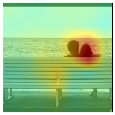
(a)

A couple

sitting on a bench looking at the sea.

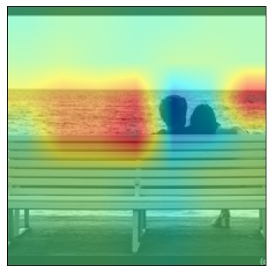
(b) A couple sitting on a bench looking at the sea .

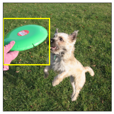
(c) A dog is jumping for a frisbee .

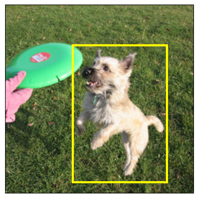
(d) A dog is jumping for a frisbee .

Figure 1: Inter-modal attributions between: (left) selected parts of a caption in yellow and an image (heatmaps over the image are red for positve and blue for negative), (right) selected bounding-boxes in the image and the caption (saliencies over captions are red for positive and blue for negative).

A hot dog sitting on a table covered in confetti.

Surrounded by glitter, there is a sausage in a bun .

A hot dog sitting on a table covered in confetti .

Surrounded by glitter , there is a sausage in a bun .

Figure 2: Intra-modal text-text attributions between top and bottom captions (top: selections in yellow, bottom: saliencies as above).

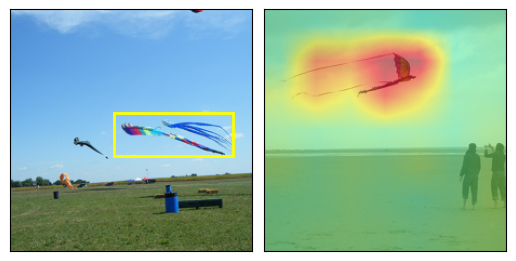
Figure 3: Intra-modal image-image attributions between left and right image (left: selection in yellow, right: heatmaps as above). More examples in Figure 11

2 Related work

Metric learning

refers to the task of producing embeddings reflecting the similarity between inputs [33]. Applications include face identification [27, 71] and image retrieval [80, 24]. Siamese networks with cosine similarity of embeddings were early candidates [10]. The triplet-loss [29] involving negative examples has been proposed as an improvement but requires sampling strategies for the large number of possible triplets [58]. Qian et al. have shown that the triplet-loss can be relaxed to a softmax variant [55]. Sohn [63] and Oord et al. [68] have proposed the batch contrastive objective which has been applied in both unsupervised [8] and supervised representation learning [34] and has lead to highly generalizable image [28] and semantic text embeddings [57].

Vision-language models

process both visual and linguistic inputs. Qi et al. were the first to train a dual-encoder architecture with a contrastive objective on image-text data in the medical domain [81]. With CLIP Radford et al. have applied this principle to web-scale image captions [56] and the ALIGN model has achieved similar results with alt-text [32]. In the following, the basic inter-modal contrastive loss has been extended by, intra-modal loss terms [25, 36, 74], self-supervision [49], non-contrastive objectives [82], incorporating classification labels [75], textual augmentation [20], a unified multi-modal encoder architecture [51] and retrieval augmentation [72]. Next to more advanced training objectives, other works have identified the training data distribution to be crucial to performance: Gadre et al. have proposed the DataComp benchmark focusing on dataset curration while fixing model architecture and training procedure [23], Xu et al. balance metadata distributions [73] and Fang et al. propose data filtering networks for the purpose [21]. The strictly separated dual-encoder architecture has been extended to include cross-encoder dependencies [39, 54], and multi-modal encoders have been combined with generative decoders [9, 45, 40, 35, 2]. The CoCa model combines contrastive learning on uni-modal vision- and text-representations with a text generative cross-modal decoder [79].

Visual-linguistic grounding

​is the identification of fine-grained relations between text phrases and corresponding image parts [12]. Specialized models predict regions over images for a corresponding input phrase [59, 77]. This objective has been combined with contrastive caption matching [41, 13], and caption generation [76]. The VoLTA model internally matches latent image-region and text-span representations while using different training objectives [54]. In multi-modal text generative models, grounding has been included as an additional pretraining task [37, 64, 11]; alternatively grounding abilities can be unlocked with visual prompt learning [16]. In this paper, we do not optimize models to predict image regions, but aim at diagnosing to what extent purely contrastively trained dual encoders have this ability.

Local feature attribution methods

aim at explaining a given prediction by assessing contributions to individual input features [50, 17, 43, 4]. First-order gradients can approximate a prediction’s sensitivity to such features [38]. In transformer architectures, attention weights were proposed as explanations [1], but ultimately rejected as only one part of the model[30, 70, 6]. Layer-wise relevance propagation (LRP) defines layer-specific rules to back-propagate attributions to individual features [48, 5]. In contrast shapley values [46] and Integrated Gradients (IG) [66] treat models holistically and can provide a form of theoretical guaranty for correctness. This has recently been challenged by Bilodeau et al. who prove fundamental limitations of attribution methods [7]. A popular attribution method in the vision domain is GradCam [61]. In Appendix D we discuss the relation between IG, GradCam and our work.
First-order attribution methods including the above, cannot capture dependencies on feature interactions. Tsang et al. have proposed to detect such interactions from weight matrices in feed-forward neural netorks [67], the Shapley value has been extended to the Shapley Interaction Index [26, 65, 22] and Janizek et al. have generalized IG to integrated Hessians [31]. A special case are dual and Siamese encoders whose predictions only depend on feature interactions between the final embeddings of two inputs coming from otherwise entirely independent encoders (cf. Eq. 1). Eberle et al. have extended LRP for this model class [19, 69]. Möller et al. have extended IG to Siamese language encoders [52, 47]. Here we further generalize this work to multi-modal dual encoders.

3 Method

We first derive general feature-pair attributions for dual encoder predictions and then specifically apply the result to vision-language models.

Derivation of feature-pair attributions.

Let

$$f(\mathbf{a},\mathbf{b})=\mathbf{g}(\mathbf{a})^{T}\mathbf{h}(\mathbf{b})=s$$ (1)

be a differentiable dual-encoder model, with two vector-valued encoders $\mathbf{g}$ and $\mathbf{h}$, respective inputs $\mathbf{a}$ and $\mathbf{b}$ and a scalar output $s$. For our purpose, $\mathbf{g}$ will be an image encoder with an image input $\mathbf{a}$ and $\mathbf{h}$ will be a text encoder with a text representation $\mathbf{b}$ as input. To attribute the prediction $s$ onto features of the two inputs $\mathbf{a}$ and $\mathbf{b}$, we also define two uninformative reference inputs $\mathbf{r}_{a}$, the black image, and $\mathbf{r}_{b}$, a sequence of padding tokens with fixed length. We then start from the following expression:

$$f(\mathbf{a},\mathbf{b})-f(\mathbf{r}_{a},\mathbf{b})-f(\mathbf{a},\mathbf{r}_{b})+f(\mathbf{r}_{a},\mathbf{r}_{b})$$ (2)

Interpreting $f$ as an anti-derivative, we can reformulate it into an integral over the derivative of $f$:

$$\begin{split}&\big{[}f(\mathbf{a},\mathbf{b})-f(\mathbf{r}_{a},\mathbf{b})\big{]}-\big{[}f(\mathbf{a},\mathbf{r}_{b})-f(\mathbf{r}_{a},\mathbf{r}_{b})\big{]}\\[2.15277pt] =\int_{\mathbf{r}_{b}}^{\mathbf{b}}\,\frac{\partial}{\partial\mathbf{y}_{j}}\,&\big{[}f(\mathbf{a},\mathbf{y})-f(\mathbf{r}_{a},\mathbf{y})\big{]}\,d\mathbf{y}_{j}=\int_{\mathbf{r}_{b}}^{\mathbf{b}}\!\int_{\mathbf{r}_{a}}^{\mathbf{a}}\frac{\partial^{2}}{\partial\mathbf{x}_{i}\partial\mathbf{y}_{j}}\,f\left(\mathbf{x},\mathbf{y}\right)\,d\mathbf{x}_{i}\,d\mathbf{y}_{j}\end{split}$$ (3)

Here, $\mathbf{x}$ and $\mathbf{y}$ are integration variables for the two inputs and we use component-wise notation with the indices $i$ and $j$ for the input dimensions and omit sums over double indices for clarity. We plug in the model definition from Equation 1:

$$\int_{\mathbf{r}_{a}}^{\mathbf{a}}\!\int_{\mathbf{r}_{b}}^{\mathbf{b}}\frac{\partial^{2}}{\partial\mathbf{x}_{i}\partial\mathbf{y}_{j}}\,\mathbf{g}_{k}(\mathbf{x})\,\mathbf{h}_{k}(\mathbf{y})\,d\mathbf{x}_{i}\,d\mathbf{y}_{j}$$ (4)

Again, we use component-wise notation for the dot-product between the two embeddings $\mathbf{g}(\mathbf{x})$ and $\mathbf{h}(\mathbf{y})$ and index output dimensions with $k$. Since neither embedding depends on the other integration variable, we can separate the expression into:

$$\int_{\mathbf{r}_{a}}^{\mathbf{a}}\frac{\partial\mathbf{g}_{k}(\mathbf{x})}{\partial\mathbf{x}_{i}}\,d\mathbf{x}_{i}\int_{\mathbf{r}_{b}}^{\mathbf{b}}\frac{\partial\mathbf{h}_{k}(\mathbf{y})}{\partial\mathbf{y}_{j}}\,d\mathbf{y}_{j}$$ (5)

This step makes explicit use of the strict separation of the two encoders. Cross-encoder architectures would introduce dependencies between them. Both terms are line integrals from the references to the actual inputs in the respective input representation spaces; $\partial\mathbf{g}_{k}(\mathbf{x})/\partial\mathbf{x}_{i}$ and $\partial\mathbf{h}_{k}(\mathbf{y})/\partial\mathbf{y}_{j}$ are the Jacobians of the two encoders. Following the concept of integrated gradients [66], we define the straight lines between both references and inputs,

$$\mathbf{x}(\alpha) =\mathbf{r}_{a}+\alpha(\mathbf{a}-\mathbf{r}_{a}),$$ (6)

$$\mathbf{y}(\beta) =\mathbf{r}_{b}+\beta(\mathbf{b}-\mathbf{r}_{b}),$$ (7)

parameterized by $\alpha$ and $\beta$, and solve by substitution. For the integral over encoder $\mathbf{g}$ this yields

$$\int_{0}^{1}\frac{\partial\mathbf{g}_{k}\left(\mathbf{x(\alpha})\right)}{\partial\mathbf{x}_{i}}\,\frac{\partial\mathbf{x}_{i}(\alpha)}{\partial\alpha}\,d\alpha\,=\,(\mathbf{a}-\mathbf{r}_{a})_{i}\int_{0}^{1}\frac{\partial\mathbf{g}_{k}\left(\mathbf{x(\alpha})\right)}{\partial\mathbf{x}_{i}}\,d\alpha,$$ (8)

since $\partial\mathbf{x}(\alpha)/\partial\alpha=(\mathbf{a}-\mathbf{r}_{a})$, which is a constant w.r.t $\alpha$; hence, we can pull it out of the integral. The integral over encoder $\mathbf{h}$ is processed in the same way. We then define the two integrated Jacobians,

$$\mathbf{J}_{ki}^{a}=\int_{0}^{1}\frac{\partial\mathbf{g}_{k}\left(\mathbf{x(\alpha})\right)}{\partial\mathbf{x}_{i}}\,d\alpha\approx\frac{1}{N}\,\sum_{n=1}^{N}\,\frac{\partial\mathbf{g}_{k}(\mathbf{x}(\alpha_{n}))}{\partial\mathbf{x}_{i}},$$ (9)

and $\mathbf{J}_{kj}^{b}$ analogously. In practice, these integrals are calculated numerically by sums over $N$ steps, with $\alpha_{n}=n/N$. This introduces an approximation error which must, however, converge to zero for large $N$ by definition of the Riemann integral. We plug the results from Equation 8 and the definitions of the integrated Jacobians back into Equation 5 and obtain:

$$(\mathbf{a}-\mathbf{r}_{a})_{i}\,\mathbf{J}_{ik}^{a}\mathbf{J}_{kj}^{b}\,(\mathbf{b}-\mathbf{r}_{b})_{j}\eqcolon\mathbf{A}_{ij}$$ (10)

After computing the sum over the output embedding dimensions $k$, this provides a matrix of feature-pairs $(i,j)$ in input $\mathbf{a}$ and $\mathbf{b}$ which we call attribution matrix $\mathbf{A}_{ij}$. Note that except for the numerical integration, the equality to Equation 2 still holds. Hence, the sum over all feature-pair attributions in $\mathbf{A}$ is an exact reformulation of the ansatz. If the references $\mathbf{r}_{a}$ and $\mathbf{r}_{b}$ are uninformative, i.e. $f(\mathbf{r}_{a},\mathbf{b})\approx 0,\,f(\mathbf{a},\mathbf{r}_{b})\approx 0,\,f(\mathbf{r}_{a},\mathbf{r}_{b})\approx 0,$ we arrive at the final approximation

$$f(\mathbf{a},\mathbf{b})\approx\sum_{ij}\mathbf{A}_{ij},$$ (11)

where $i$ ranges over dimensions in input $\mathbf{a}$ and $j$ over $\mathbf{b}$. This provides an approximate decomposition of the model prediction $s\!=\!f(\mathbf{a},\mathbf{b})$ into additive contributions of feature-pairs in the two inputs.

Inter-modal attributions.

In the derivation above, we treat image and text representations as vectors. In current transformer-based language encoders, text inputs are represented as $S\!\times\!D_{b}$ dimensional tensors, where $S$ is the length of the token sequence and $D$ is the model’s embedding dimensionality. In vision transformers, image representations are $P\!\times\!P\!\times\!D_{a}$ dimensional tensors, with $P$ being the number of patches that the image is split into horizontally and vertically. Our pair-wise image-text attributions thus have the dimensions $P\!\times\!P\!\times\!D_{a}\!\times\!S\!\times\!D_{b}$. With hundreds of embedding dimensions and tens of tokens and patches, this quickly becomes intractable. Fortunately, the sum over dimensions in Equation 11 enables the additive combination of attributions in $\mathbf{A}$. We sum over the embedding dimensions of both encoders $D_{a}$ and $D_{b}$ and obtain a $P\!\times\!P\!\times\!S$ dimensional attribution tensor, which estimates for each pair of a text token and an image patch how much their combination contributes to the overall prediction. These attributions are still three-dimensional and thus not straightforward to visualize. However, again we can use their additivity, slice the 3d attribution tensor along text or image dimensions and project onto the remaining dimensions by summation. We can for example select a slice over a range of tokens and project it onto the image as in Equation 1 (a)/(b). Attribution heat maps over the image result from interpolating the patch-level attributions to the image resolution. Importantly, the two visualizations shown here come from the same 3d attribution tensor for the given caption-image pair. The reverse case of slicing parts of the image and projecting the result onto the caption dimension is shown in Equation 1(c)/(d). Here, we project the selected image slices marked by yellow bounding boxes onto the caption and visualize attributions as saliency maps over tokens in the caption.

Intra-modal attributions.

Albeit vision-language dual-encoders are typically trained to match images against captions, we can compute attributions for image-image or text-text pairs as well by applying the same encoder to both inputs. For text-text attributions, after summation over embedding dimensions, this yields an $S_{1}\!\times\!S_{2}$ dimensional attribution tensor, with $S_{1}$ and $S_{2}$ being token sequence lengths of the two texts. These 2d attributions may be visualized in the form of a matrix [52]. In Figure 2 we, however, stick to the slice representation and attribute the yellow selected slice in the first caption onto the second caption. For image-image similarities, attribution tensors become four dimensional taking the shape $(P\!\times\!P)_{1}\!\times\!(P\!\times\!P)_{2}$ and containing a contribution for every pair of two patches from either image. Parentheses indicate which input the dimensions belong to. In Figure 3, we attribute the slice of the yellow bounding-box in the left image onto the image to its right. Appendix A includes additional examples.

4 Experiments

In our experiments, we apply our feature-pair attributions to contrastively trained vision-language dual encoders. We focus on evaluating interactions of mentioned objects in captions and corresponding regions in images by selecting sub-strings in captions and attributing them onto images as in Figure 1 (left part).

4.1 Experimental setup

Datasets.

We base this evaluation on three image-caption datasets that also contain object bounding-box annotations in images, namely Microsoft’s Common Objects in Context (COCO) [42], the Flickr30k collection [78] with the entity annotations created by Plummer et al. [53], and the Hard Negative Captions (HNC) dataset by Dönmez et al. [15], which automatically generates captions from scene graphs using templates. In the attempt to minimize the domain gap between all three datasets, we sample sub-graph triplets and use a basic "<subject> <predicate> <object>"-template to create captions. In our analysis, HNC is only used for evaluation; on Flickr30k we use the official test split and on COCO we use the validation-split, as the official test-split does not contain captions.

Models.

We analyze CLIP dual-encoder architectures [56] without cross-encoder dependencies (a requirement of our method, cf. Equation 5) and the standard inter-modal contrastive objective. We evaluate the original OpenAI models which are trained on an undisclosed dataset, as well as the OpenCLIP re-implementations trained on the Laion [60], Dfn [21], CommonPool and DataComp [23] datasets, as well as MetaCLIP [73] .

Fine-tuning.

Next to evaluating the vision and language grounding capabilities of off-the-shelf CLIP models pre-trained on web-data, we are also interested in how this ability changes with access to higher-quality human annotations. We fine-tune models on the COCO and Flickr30k train splits for five epochs using the AdamW optimizer [44] with an initial learning rate of $110-7$, exponentially increasing to $110-5$, a weight decay of $110-4$, and a batch size of $64$ on one NVIDIA A6000 GPU. All fine-tunings are performed in the standard contrastive setting. We never change model architectures or training objectives to explicitly perform grounding.

4.2 Object bounding-box attributions

To systematically assess the visual-linguistic grounding abilities of the analyzed dual encoders, we evaluate the agreement of our attributions with corresponding object bounding boxes. For this experiment, we apply the following filters to the three datasets: We use a given object annotation if a single instance of its class appears in the image and its bounding-box is larger than one patch. For COCO, we identify class occurrences in the caption through a dictionary based synonym matching. For HNC, classes exactly match sub-strings in captions and in Flickr30k, respective spans are already annotated. This results in 3.5k image-caption pairs from COCO, 8k pairs from Flickr30k, and 500 pairs from HNC.

We compute attributions between the selected token range of the class caption and the image. We then scale the bounding-boxes to patch-resolution, restrict attributions to positive contributions to enable a meaningful normalization, and calculate the fraction of attributions falling inside a given bounding-box over the total attribution to the full image; we refer to this fraction as $\gamma$. Note that this procedure differs from the typical grounding evaluation [41] as we analyze dual encoders and do not train models to produce bounding-box or mask outputs.

To gain an intuition for $\gamma$-values, Figure 4 shows examples from different ranges. Very high values, like for the elephant in (d) unambiguously indicate object correspondence. Very low values on the other hand, like for the dog in (a) that is mistaken with an object that is difficult to identify in the background, are clear failure cases. Intermediate values, however, often arise from attributions extending to the context beyond the bounding box, such as the shirt in (b) and the tennis court in (c). A qualitative discussion of error cases follows below.

Figure 5 (Left) shows cumulative $\gamma$-distributions for the OpenClip models on the COCO dataset (distributions for the OpenAI models and the Flickr30k dataset are included in Appendix B). Table 1 summarizes these distributions into values for $\gamma\!>\!0.8$ and $\gamma\!>\!0.5$ for different models by OpenAI on all datasets. Additionally, it reports the fraction of cases for which the maximally attributed patch lies within the objects’ bounding-box $\rho$. Table 2 reports results in the same format for the different OpenCLIP training configurations that are all based on the ViT-B-16 architecture. We compare the grounding ability of two models by assessing their full $\gamma$-distributions and test whether the stochastic dominance of one over the other is significant [18] (details in Appendix C).
Among then OpenAI models, the improvements of the ViT-B/16 over the ViT-B/32 and RN50 models are significant at $p\!<\!0.005$ and $\epsilon\!=\!0.2$ on all three datasets except for ViT-B/32 on HNC. For both the OpenAI and OpenCLIP models, fine-tuning increases grounding abilities by a large margin when compared to unmodified models. These improvements are consistently significant at a very strict criterion of $p\!<\!0.001$ and $\epsilon\!=\!0.01$.

While the unmodified CLIP ViT-B/16 model already has good grounding abilities on COCO and Flickr30k (the examples in Figure 4 are from this model), the off-the-shelf OpenCLIP counterparts perform rather badly. However, their improvement upon in-domain fine-tuning is remarkable, which is apparent in Figure 7. The off-the-shelf model cannot identify the clock and even attributes the surfboard negatively, while the fine-tuned version points out both clearly.

To test the knowledge about specific visual-linguistic concepts in the models and how it changes upon in-domain tuning, we can break down the above analysis for individual classes. Figure 6 shows average $\gamma$-values and their standard deviations in the OpenClip Dfn model for all COCO classes, ordered from left to right by how good their average grounding ability is in the unmodified model (blue). Values for $\gamma$ range from $0.92\!\pm\!0.08$ for sheep to $0.07\!\pm\!0.07$ for snowboard. The model can already point out the leftmost classes sheep, bear, elephant etc. very well, while for the rightmost classes snowboard, cell phone, baseball bat, etc., intrinsic grounding is bad. Upon fine-tuning (orange) most classes improve. Using the standardized mean difference of the two $\gamma$-values as a measure for effect size, we observe the largest improvements for the classes horse, bench, giraffe, airplane and clock. In Appendix B (Figure 15), we repeat this experiment for the Laion and CommonPool models and observe a similar result, though, with changes in the order of classes, which we expect due to the different training data distributions.

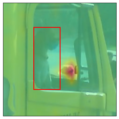
(a)

Dog

sitting inside the cab of a yellow truck. ($\gamma\!=\!0.1$)

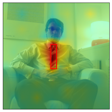
(b) A man in a shirt and tie sitting on a white chair. ($\gamma\!=\!0.4$)

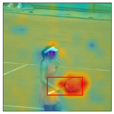
(c) Woman smiling on the court while holding her tennis racket . ($\gamma\!=\!0.5$)

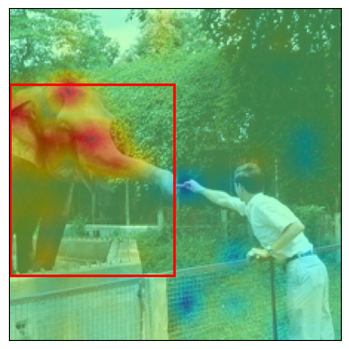
(d) A man is feeding an elephant over a fence. ($\gamma\!=\!0.9$)

Figure 4: Examples for attribuitions between selected objects in the caption (yellow) and the image together with corresponding COCO bounding-boxes. $\gamma$ is the fraction of attributions falling inside the box as described in Section 4.2.

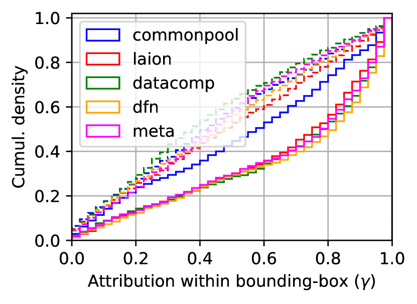
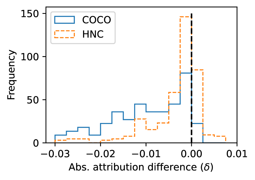
Figure 5: (Left) Cumulative distributions of the fraction of attributions falling within corresponding COCO object bounding-boxes as described in Section 4.2. (Right) Distribution of attribution differences between negative and positive captions as described in Section 4.4.

Table 1: Summary of the vision-language grounding evaluation for different CLIP models by OpenAI as described in Section 4.2. Model refers to the investigated architecture, tuning is whether the model was fine-tuned on the train split of the respective dataset, $\gamma_{>x}$ reports cumulative $\gamma$-densities for values larger than $x$ (cf. Figure 5 left) and $\rho$ is the fraction of cases where the maximally attributed patch falls inside the object bounding-box.

		COCO			HNC			Flickr30k
Model	tuning	$\gamma_{>0.5}$	$\gamma_{>0.8}$	$\rho$	$\gamma_{>0.5}$	$\gamma_{>0.8}$	$\rho$	$\gamma_{>0.5}$	$\gamma_{>0.8}$	$\rho$
RN50	No	66.3	28.8	76.9	50.1	22.6	61.8	60.1	25.5	71.2
ViT-B/32	No	63.5	33.3	69.1	52.8	28.5	58.5	50.4	23.4	58.1
ViT-B/16	No	72.3	35.7	79.0	57.0	31.7	65.0	64.4	28.4	72.1
ViT-B/16	Yes	78.0	48.4	82.9	-	-	-	73.4	40.7	79.0

Table 2: Summary of the vision-language grounding evaluation for all OpenClip models. The Training column refers to the dataset the model was initially trained on. All models implement the ViT-B-16 architecture except Meta-Clip that uses quickgelu activations. Otherwise the format is as in Table 1

		COCO			Flickr30k
Training	Tuning	$\gamma_{>0.5}$	$\gamma_{>0.8}$	$\rho$	$\gamma_{>0.5}$	$\gamma_{>0.8}$	$\rho$
Laion	No	49.4	22.0	63.3	38.2	15.9	52.0
	Yes	71.1	47.3	83.2	54.6	30.6	61.8
CommonPool	No	43.0	18.2	58.8	36.7	15.5	53.0
	Yes	57.7	28.7	67.1	44.6	20.8	56.2
DataComp	No	38.5	14.6	56.0	32.8	11.8	48.9
	Yes	72.4	50.0	75.1	50.7	27.3	56.0
DFN	No	46.5	19.6	54.3	35.4	12.3	43.3
	Yes	71.4	53.3	74.6	53.1	33.5	58.3
Meta-Clip	No	44.2	16.8	52.3	37.0	14.5	46.4
	Yes	57.5	49.8	77.1	49.2	24.1	57.2

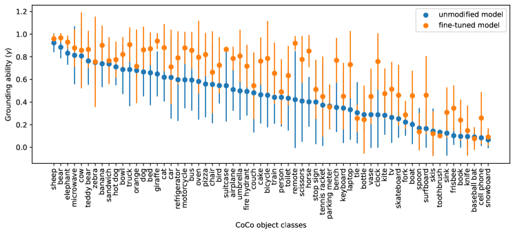
Figure 6: Class wise average grounding ability ($\gamma$) and its standard deviation (error bars) of the OpenClip DFN model before and after in-domain fine-tuning on the COCO train split.

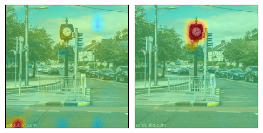
(a) A clock on a pole in the intersection of two streets.

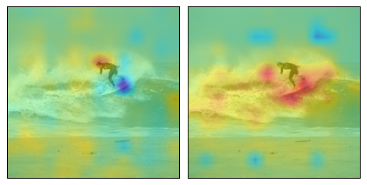
(b) A surfer riding a wave on a yellow surfboard .

Figure 7: Attribution differences between the off-the-shelf OpenCLIP model (left image) and a version fine-tuned on COCO (right image). Attribution heat maps are for selected caption parts in yellow.

4.3 Attributions to other objects

In many of the above examples, we observe that when selecting objects in the caption and attributing to the image, or vice versa, other objects that also occur in the caption and appear in the image, often receive negative attributions. Figure 8 includes four explicit cases of selected objects in a caption (yellow) receiving positive attributions in the image and other objects (underlined) that are attributed negatively. For a systematic evaluation of this effect, we sample instances from COCO that include at least two different object classes, which both appear exactly once in the image and are mentioned in the caption. We select one of them and compute the total attribution to its actual bounding-box as well as the attribution to the other object’s bounding box. We then repeat this evaluation with the second object. The attribution to the actual bounding-box is almost always positive ($97.1\%$), while the attribution to the other bounding-box receives a negative attribution in $65.6\%$ of the cases. In the model fine-tuned on COCO, this fraction increases to $70.1\%$. A distribution over the sign of attributions is included as Figure 12 in the Appendix. This shows that the models do indeed often attribute other objects negatively, however, this is not always the case.

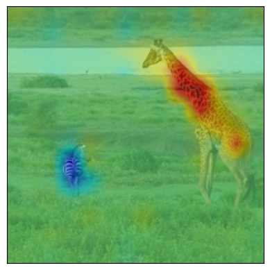
(a) A giraffe and a zebra checking each other out.

(b) A desk with items including a cellphone and pocket change.

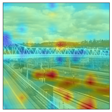
(c) A long bridge with a train going underneath.

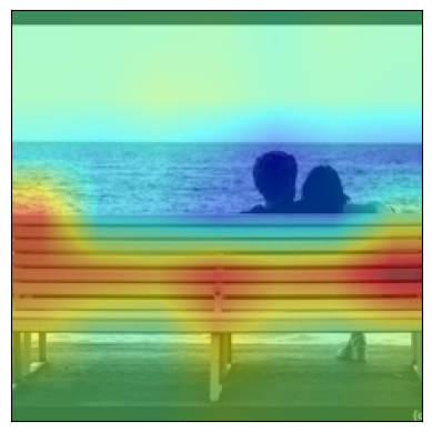
(d) A couple sitting on a bench looking at the sea.

Figure 8: Attributions between selected parts of a caption (yellow) and a corresponding image. Other objects that also appear in the image and are mentioned in the caption (underlined) but are not selected for attribution often receive negative attributions (blue parts of the attribution heatmaps).

4.4 Hard Negative Captions

We extend the grounding evaluation by creating hard negative captions that replace an object in a positive caption with a reasonable but different object to receive a negative counterpart. Dönmez et al. [15] proposed an automatic procedure to generate positive and hard negative captions, which we leverage together with our simplified template (cf. Section 4). Additionally, we create a second resource from COCO, by manually annotating a small yet high-quality evaluation sample of 100 image-caption pairs.

We then compute attributions between the token range of the original or replaced object and the object bounding-box in the image. We define the attribution difference between the negative and the positive caption as $\delta$ and show distributions over both dataset samples in Figure 5 (right). In $95.2\%$ ($74.0\%$) of the cases in COCO (HNC), this difference is negative. Therefore, the model mostly reacts correctly to the mistake in the caption and the assigned attribution decreases. Two examples are included in Figure 9. On the left, the wrong object a coffee in a mug actually receives a negative attribution for the correct object a slice of pizza on a plate in the image. On the right, the attribution to the teddy bear bounding box decreases when replacing it with book but is still clearly positive.

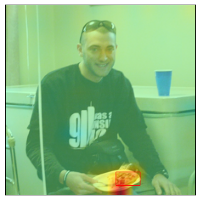
(a) A man holding a slice of pizza on a plate .

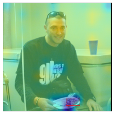
(b) A man holding a coffee in a mug .

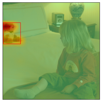
(c) A child sitting on a bed looking at a teddy bear .

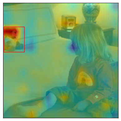
(d) A child sitting on a bed looking at a book .

Figure 9: Attributions for hard negative captions. True objects are marked yellow in the captions, replaced negative ones are marked in magenta. COCO bounding-boxes for the corresponding true object in the image are in red.

5 Discussion

Interpretation of results.

Our results show that vision-language dual-encoders can learn fine-grained correspondence between parts of captions and regions in images. This occurs despite these models’ simple architecture, incorporating a single weak interaction between vision and language embeddings via a dot-product in the final embedding space, and training objective of conventional inter-modal only contrastive matching. However, we find that this ability appears to be heavily influenced by the distribution of the pre-training data. Initially, the OpenCLIP model trained only on the Laion dataset grounds poorly but exhibits a large improvement after fine-tuning. This indicates that exposure to specific visual-linguistic concepts is necessary for models to develop robust inter-modal correspondences. As the original CLIP models perform much better on these datasets, we hypothesize that the COCO and Flickr30k training splits are included in their pretraining. Future work should analyze whether this grounding ability generalizes better in larger models.

An interesting finding is that models do not only learn fine-grained visual-linguistic correspondence for objects but often actively down-weight mismatches with negative attributions (Section 4.3). Our evaluation with hard negative captions shows that overall the models correctly react to errors in captions and can even clearly point out mismatches between wrong captions and images in some cases. However, this is not consistently the case, which suggests that models may benefit from including hard negative captions into the training procedure.

Failure cases.

The off-the-shelf OpenCLIP models frequently show obvious misattributions on all test sets (cf. Figure 7). In contrast, the fine-tuned models (including the OpenAI off-the-shelf CLIP models) exhibit hardly any clearly wrong attributions anymore. Qualitatively, errors leading to low values of $\gamma$ in these models include: true misidentifications of objects in difficult scenes (cf. the dog in Figure 4), partial covering of objects, attributions extending outside of bounding boxes onto neighboring patches, and spread-out attributions in visually strongly correlated contexts like bathrooms, kitchens, tennis courts, etc. (cf. Figure 10 for examples). We also observe cases suggesting that the models do not have an understanding of exclusivity: single objects in captions can be attributed to different objects in the image or vice-versa, e.g. the car and bus in Figure 10.

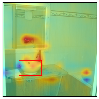
(a) A bathroom with a sink . $\gamma\!=\!0.17$

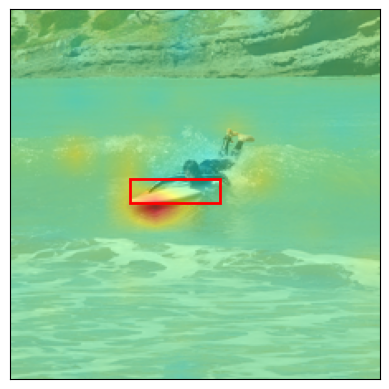
(b) Somone is going down a wave lying on a surfboard belly down. $\gamma\!=\!0.1$

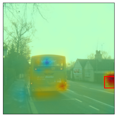
(c) A yellow bus and a red car on a street. $\gamma\!=\!0.08$

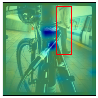
(d) A waiting person behind a locked bicycle. $\gamma\!=\!0.1$

Figure 10: Different error cases with low $\gamma$-values as discussed in Section 5. COCO bounding-boxes (red) are for corresponding token-ranges (yellow).

Limitations.

Our feature-pair attributions are an approximation as Equation 11 states clearly. Moreover, throughout this work, we attribute to deep representations of inputs because it is computationally feasible and informative [47]. In both vision and language (transformer) encoders, deep representations have undergone multiple contextualization steps and are technically not bound to input features at the given position anymore. Last, recently proven fundamental limitations of attribution methods urge caution in their interpretation, especially, regarding counterfactual conclusions about the importance of individual features for the overall prediction [7]. Despite these considerations, empirically, our evaluations show that our derived feature-pair attributions produce reasonable results in a large majority of cases and can point out inabilities (of the OpenClip model), errors (misidentification of objects), and biases (contextualization in correlated scenes). While they should not be seen as guaranteed robust and faithful explanations, we argue that they do provide valuable insights into dual-encoder models and have the potential to improve these models further.

6 Conclusion

In this paper, we have derived general feature-pair attributions for differentiable dual-encoder architectures which can attribute similarity predictions for two inputs onto interactions of their features. Our attribution method applies to any dual-encoder architecture in arbitrary domains. We believe the method can lead to valuable insights in other applications like image similarity or (multi-modal) information-retrieval and help improve these models further.

We have furthermore applied our method to contrastively trained vision-language models in order to evaluate whether such models can relate objects in captions and images. We found that they can learn fine-grained correspondence between visual and linguistic concepts. Mis-matches are often not only ignored, but negatively down-weighted instead. However, this inter-modal correspondence can be poor when models are not exposed to matching data distributions during pre-training. Finally, our analysis indicates that contrastive vision-language training may be improved by incorporating hard negative captions and by de-coupling strongly correlated objects (e.g. in scenes like bathrooms or streets).

Appendix A Additional Examples

Figure 11 shows two more examples for image-image attributions as described in Section 3.

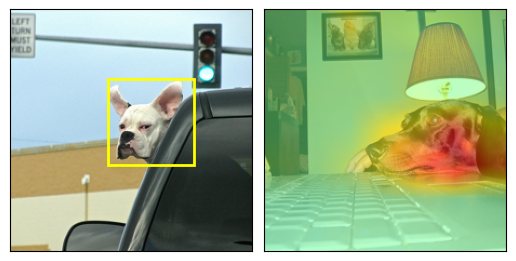
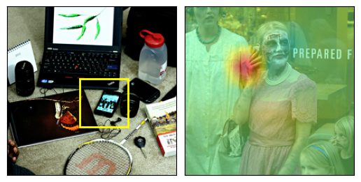
Figure 11: Image-image attributions between the yellow bounding-box in the left image and the one to its right as described in Section 3

Appendix B Additional plots

Figure 12 shows the distribution of attribution signs that the analysis in Section 4.3 is based on. Figure 13 and 15 provide additional plots of cumulative $\gamma$-distributions for different models and datasets and Figure 15 shows class wise evaluations of $\gamma$ for two additional models.

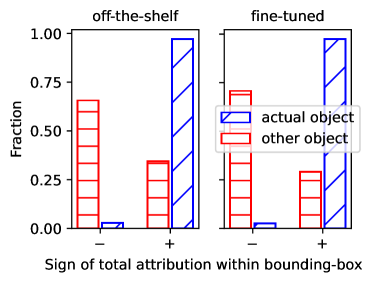
Figure 12: Distribution of signs of attributions to actual and other objects in the image as described in Section 4.3.

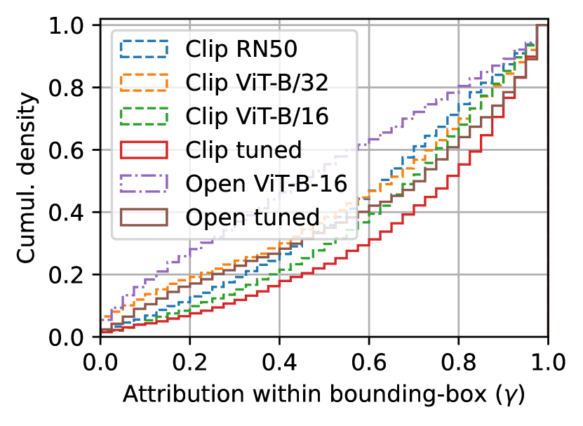
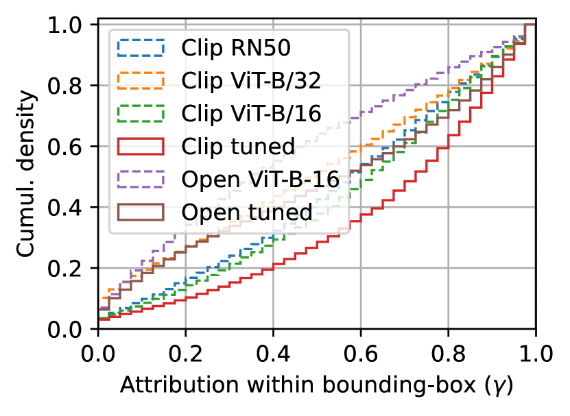
Figure 13: Cumulative $\gamma$-distribution plots of the OpenAI models for the Coco (left) and Flickr30k (right) dataset as described in Section 4.2.

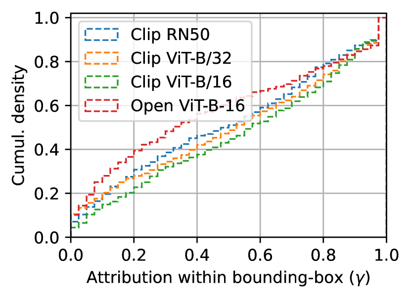
Figure 14: Cumulative $\gamma$-distribution plots for the OpenAI models on HNC (left) and then OpenCLIP models on Flickr30k (right) as described in Section 4.2.

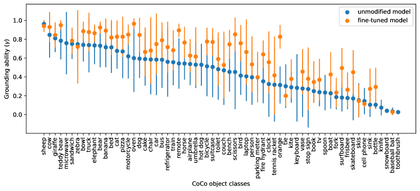
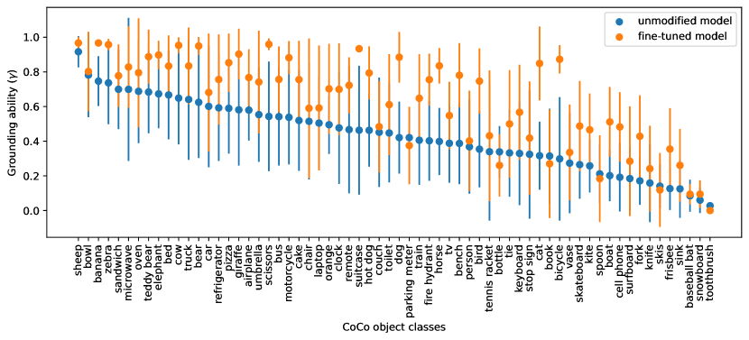
Figure 15: Class wise evaluation of intrinsic grounding ($\gamma$) in the OpenCLIP Laion (top) and DataComp (bottom) as discussed in Section 4.2, cf. Figure 6.

Appendix C Stochastic Dominance

Stochastic dominance or order is a framework to compare cumulative distributions. DelBarrio et al. [14] have proposed a significance test building on the principle and Dror et al. [18] have identified it as being particularly suitable to compare deep neural models. The test’s $\epsilon$-parameter is the maximal percentile range where the inferior distribution is allowed to dominate the superior one and Dror et al. suggest to set it to $\epsilon<0.4$. The smaller $\epsilon$, the stricter the criterion. $\alpha$ is the significance level.

Appendix D Relation to GradCam

We now discuss the relation of integrated gradients [66] and GradCam. We start by deriving IG for a model $f(\mathbf{a})=s$ with a vector-valued input $\mathbf{a}$ and a scalar prediction $s$, which might e.g. be a classification score for a particular class. We define the reference input $\mathbf{r}$, begin from the difference between the two predictions and reformulate it as an integral:

$$f(\mathbf{a})-f(\mathbf{r})=\int_{\mathbf{r}}^{\mathbf{a}}\frac{\partial f(\mathbf{x})}{\partial\mathbf{x}_{i}}d\mathbf{x}_{i}$$ (12)

To solve the resulting line integral, we substitute with the straight line $\mathbf{x}(\alpha)=\mathbf{r}+\alpha(\mathbf{a}-\mathbf{r})$ and pull its derivative $d\mathbf{x}(\alpha)/d\alpha=(\mathbf{a}-\mathbf{r})$ out of the integral:

$$\int_{\alpha=0}^{1}\frac{\partial f(\mathbf{x}(\alpha))}{\partial\mathbf{x}_{i}(\alpha)}\frac{\partial\mathbf{x}_{i}(\alpha)}{\partial\alpha}d\alpha=(\mathbf{a}-\mathbf{r})_{i}\int_{\alpha=1}^{1}\nabla_{i}f(\mathbf{x}(\alpha))\,d\alpha$$ (13)

to arrive at the final IG we approximate the integral by a sum over $N$ steps:

$$(\mathbf{a}-\mathbf{r})_{i}\,\frac{1}{N}\sum_{n=1}^{N}\,\nabla_{i}f(\mathbf{x}(\alpha_{n}))$$ (14)

If $f(\mathbf{r})\approx 0$ this is the contribution of feature $i$ in $\mathbf{a}$ to the model prediction $f(\mathbf{a})=s$. We can now reduce these feature attributions further by setting $N=1$ and $\mathbf{r}=\mathbf{0}$, the black image to obtain

$$\mathbf{a}_{i}\nabla_{i}f(\mathbf{a}),$$ (15)

which is basic form of GradCam. The method typically attributes to deep image representations in CNNs, so that $\mathbf{a}$ have the dimensions $C\!\times\!H\!\times\!W$, the number of channles, height and width of the representation. To reduce attributions to a two-dimensional map, it sums over the channel dimension and applies a relu-activation to the outcome. The original version also average pools the gradients over the spacial dimensions, however, this is technically not necessary.

As discussed earlier, neither integrated gradients nor GradCam can explain dual encoder predictions. Following the logic from above we could, however, derive a GradCam for similarity by setting $N=1$ in the computation of the integrated Jacobians in Equation 9 and using $\mathbf{r}_{a}=\mathbf{0}$ and $\mathbf{r}_{b}=\mathbf{0}$. For our attribution matrix from Equation 10 we would then receive the simplified version

$$\mathbf{a}_{i}\,\frac{\partial\mathbf{g}_{k}}{\partial\mathbf{a}_{i}}\,\frac{\partial\mathbf{h}_{k}}{\partial\mathbf{b}_{j}}\,\mathbf{b}_{j}.$$ (16)

However, setting $N=1$ is the worst possible approximation to the integrated Jacobians. Therefore, this extreme simplification must be used with caution and should only be taken as a very rough estimate.

References

- [1] Samira Abnar and Willem Zuidema. Quantifying attention flow in transformers. In Dan Jurafsky, Joyce Chai, Natalie Schluter, and Joel Tetreault, editors, Proceedings of the 58th Annual Meeting of the Association for Computational Linguistics, pages 4190–4197, Online, July 2020. Association for Computational Linguistics.
- [2] Jean-Baptiste Alayrac, Jeff Donahue, Pauline Luc, Antoine Miech, Iain Barr, Yana Hasson, Karel Lenc, Arthur Mensch, Katherine Millican, Malcolm Reynolds, Roman Ring, Eliza Rutherford, Serkan Cabi, Tengda Han, Zhitao Gong, Sina Samangooei, Marianne Monteiro, Jacob L Menick, Sebastian Borgeaud, Andy Brock, Aida Nematzadeh, Sahand Sharifzadeh, Mikoł aj Bińkowski, Ricardo Barreira, Oriol Vinyals, Andrew Zisserman, and Karén Simonyan. Flamingo: a visual language model for few-shot learning. In S. Koyejo, S. Mohamed, A. Agarwal, D. Belgrave, K. Cho, and A. Oh, editors, Advances in Neural Information Processing Systems, volume 35, pages 23716–23736. Curran Associates, Inc., 2022.
- [3] Stanislaw Antol, Aishwarya Agrawal, Jiasen Lu, Margaret Mitchell, Dhruv Batra, C Lawrence Zitnick, and Devi Parikh. Vqa: Visual question answering. In Proceedings of the IEEE international conference on computer vision, pages 2425–2433, 2015.
- [4] Pepa Atanasova, Jakob Grue Simonsen, Christina Lioma, and Isabelle Augenstein. A diagnostic study of explainability techniques for text classification. In Bonnie Webber, Trevor Cohn, Yulan He, and Yang Liu, editors, Proceedings of the 2020 Conference on Empirical Methods in Natural Language Processing (EMNLP), pages 3256–3274, Online, November 2020. Association for Computational Linguistics.
- [5] Sebastian Bach, Alexander Binder, Grégoire Montavon, Frederick Klauschen, Klaus-Robert Müller, and Wojciech Samek. On pixel-wise explanations for non-linear classifier decisions by layer-wise relevance propagation. PloS one, 10(7):e0130140, 2015.
- [6] Jasmijn Bastings and Katja Filippova. The elephant in the interpretability room: Why use attention as explanation when we have saliency methods? In Afra Alishahi, Yonatan Belinkov, Grzegorz Chrupała, Dieuwke Hupkes, Yuval Pinter, and Hassan Sajjad, editors, Proceedings of the Third BlackboxNLP Workshop on Analyzing and Interpreting Neural Networks for NLP, pages 149–155, Online, November 2020. Association for Computational Linguistics.
- [7] Blair Bilodeau, Natasha Jaques, Pang Wei Koh, and Been Kim. Impossibility theorems for feature attribution. Proceedings of the National Academy of Sciences, 121(2):e2304406120, 2024.
- [8] Mathilde Caron, Ishan Misra, Julien Mairal, Priya Goyal, Piotr Bojanowski, and Armand Joulin. Unsupervised learning of visual features by contrasting cluster assignments. Advances in neural information processing systems, 33:9912–9924, 2020.
- [9] Xi Chen, Xiao Wang, Soravit Changpinyo, AJ Piergiovanni, Piotr Padlewski, Daniel Salz, Sebastian Goodman, Adam Grycner, Basil Mustafa, Lucas Beyer, Alexander Kolesnikov, Joan Puigcerver, Nan Ding, Keran Rong, Hassan Akbari, Gaurav Mishra, Linting Xue, Ashish V Thapliyal, James Bradbury, Weicheng Kuo, Mojtaba Seyedhosseini, Chao Jia, Burcu Karagol Ayan, Carlos Riquelme Ruiz, Andreas Peter Steiner, Anelia Angelova, Xiaohua Zhai, Neil Houlsby, and Radu Soricut. PaLI: A jointly-scaled multilingual language-image model. In The Eleventh International Conference on Learning Representations, 2023.
- [10] Xinlei Chen and Kaiming He. Exploring simple siamese representation learning. In Proceedings of the IEEE/CVF conference on computer vision and pattern recognition, pages 15750–15758, 2021.
- [11] Yen-Chun Chen, Linjie Li, Licheng Yu, Ahmed El Kholy, Faisal Ahmed, Zhe Gan, Yu Cheng, and Jingjing Liu. Uniter: Universal image-text representation learning. In European conference on computer vision, pages 104–120. Springer, 2020.
- [12] Zhihong Chen, Ruifei Zhang, Yibing Song, Xiang Wan, and Guanbin Li. Advancing visual grounding with scene knowledge: Benchmark and method. In Proceedings of the IEEE/CVF Conference on Computer Vision and Pattern Recognition (CVPR), pages 15039–15049, June 2023.
- [13] Samyak Datta, Karan Sikka, Anirban Roy, Karuna Ahuja, Devi Parikh, and Ajay Divakaran. Align2ground: Weakly supervised phrase grounding guided by image-caption alignment. In Proceedings of the IEEE/CVF international conference on computer vision, pages 2601–2610, 2019.
- [14] Eustasio del Barrio, Juan A. Cuesta-Albertos, and Carlos Matrán. An Optimal Transportation Approach for Assessing Almost Stochastic Order, pages 33–44. Springer International Publishing, Cham, 2018.
- [15] Esra Dönmez, Pascal Tilli, Hsiu-Yu Yang, Ngoc Thang Vu, and Carina Silberer. Hnc: Leveraging hard negative captions towards models with fine-grained visual-linguistic comprehension capabilities. In Proceedings of the 27th Conference on Computational Natural Language Learning (CoNLL), pages 364–388, 2023.
- [16] Michael Dorkenwald, Nimrod Barazani, Cees GM Snoek, and Yuki M Asano. Pin: Positional insert unlocks object localisation abilities in vlms. arXiv preprint arXiv:2402.08657, 2024.
- [17] Finale Doshi-Velez and Been Kim. Towards a rigorous science of interpretable machine learning, 2017.
- [18] Rotem Dror, Segev Shlomov, and Roi Reichart. Deep dominance - how to properly compare deep neural models. In Proceedings of the 57th ACL, pages 2773–2785, Florence, Italy, July 2019. ACL.
- [19] Oliver Eberle, Jochen Büttner, Florian Kräutli, Klaus-Robert Müller, Matteo Valleriani, and Grégoire Montavon. Building and interpreting deep similarity models. IEEE Transactions on Pattern Analysis and Machine Intelligence, 44(3):1149–1161, 2020.
- [20] Lijie Fan, Dilip Krishnan, Phillip Isola, Dina Katabi, and Yonglong Tian. Improving clip training with language rewrites. In A. Oh, T. Naumann, A. Globerson, K. Saenko, M. Hardt, and S. Levine, editors, Advances in Neural Information Processing Systems, volume 36, pages 35544–35575. Curran Associates, Inc., 2023.
- [21] Alex Fang, Albin Madappally Jose, Amit Jain, Ludwig Schmidt, Alexander T Toshev, and Vaishaal Shankar. Data filtering networks. In The Twelfth International Conference on Learning Representations, 2024.
- [22] Fabian Fumagalli, Maximilian Muschalik, Patrick Kolpaczki, Eyke Hüllermeier, and Barbara Hammer. Shap-iq: Unified approximation of any-order shapley interactions. Advances in Neural Information Processing Systems, 36, 2024.
- [23] Samir Yitzhak Gadre, Gabriel Ilharco, Alex Fang, Jonathan Hayase, Georgios Smyrnis, Thao Nguyen, Ryan Marten, Mitchell Wortsman, Dhruba Ghosh, Jieyu Zhang, Eyal Orgad, Rahim Entezari, Giannis Daras, Sarah M Pratt, Vivek Ramanujan, Yonatan Bitton, Kalyani Marathe, Stephen Mussmann, Richard Vencu, Mehdi Cherti, Ranjay Krishna, Pang Wei Koh, Olga Saukh, Alexander Ratner, Shuran Song, Hannaneh Hajishirzi, Ali Farhadi, Romain Beaumont, Sewoong Oh, Alex Dimakis, Jenia Jitsev, Yair Carmon, Vaishaal Shankar, and Ludwig Schmidt. Datacomp: In search of the next generation of multimodal datasets. In Thirty-seventh Conference on Neural Information Processing Systems Datasets and Benchmarks Track, 2023.
- [24] Xingyu Gao, Steven CH Hoi, Yongdong Zhang, Ji Wan, and Jintao Li. Soml: Sparse online metric learning with application to image retrieval. In Proceedings of the AAAI Conference on Artificial Intelligence, volume 28, 2014.
- [25] Shashank Goel, Hritik Bansal, Sumit Bhatia, Ryan Rossi, Vishwa Vinay, and Aditya Grover. Cyclip: Cyclic contrastive language-image pretraining. In S. Koyejo, S. Mohamed, A. Agarwal, D. Belgrave, K. Cho, and A. Oh, editors, Advances in Neural Information Processing Systems, volume 35, pages 6704–6719. Curran Associates, Inc., 2022.
- [26] Michel Grabisch and Marc Roubens. An axiomatic approach to the concept of interaction among players in cooperative games. International Journal of game theory, 28:547–565, 1999.
- [27] Matthieu Guillaumin, Jakob Verbeek, and Cordelia Schmid. Is that you? metric learning approaches for face identification. In 2009 IEEE 12th international conference on computer vision, pages 498–505. IEEE, 2009.
- [28] Kaiming He, Haoqi Fan, Yuxin Wu, Saining Xie, and Ross Girshick. Momentum contrast for unsupervised visual representation learning. In Proceedings of the IEEE/CVF conference on computer vision and pattern recognition, pages 9729–9738, 2020.
- [29] Elad Hoffer and Nir Ailon. Deep metric learning using triplet network. In Similarity-Based Pattern Recognition: Third International Workshop, SIMBAD 2015, Copenhagen, Denmark, October 12-14, 2015. Proceedings 3, pages 84–92. Springer, 2015.
- [30] Sarthak Jain and Byron C. Wallace. Attention is not Explanation. In Jill Burstein, Christy Doran, and Thamar Solorio, editors, Proceedings of the 2019 Conference of the North American Chapter of the Association for Computational Linguistics: Human Language Technologies, Volume 1 (Long and Short Papers), pages 3543–3556, Minneapolis, Minnesota, June 2019. Association for Computational Linguistics.
- [31] Joseph D Janizek, Pascal Sturmfels, and Su-In Lee. Explaining explanations: Axiomatic feature interactions for deep networks. Journal of Machine Learning Research, 22(104):1–54, 2021.
- [32] Chao Jia, Yinfei Yang, Ye Xia, Yi-Ting Chen, Zarana Parekh, Hieu Pham, Quoc Le, Yun-Hsuan Sung, Zhen Li, and Tom Duerig. Scaling up visual and vision-language representation learning with noisy text supervision. In Marina Meila and Tong Zhang, editors, Proceedings of the 38th International Conference on Machine Learning, volume 139 of Proceedings of Machine Learning Research, pages 4904–4916. PMLR, 18–24 Jul 2021.
- [33] Mahmut Kaya and Hasan Şakir Bilge. Deep metric learning: A survey. Symmetry, 11(9):1066, 2019.
- [34] Prannay Khosla, Piotr Teterwak, Chen Wang, Aaron Sarna, Yonglong Tian, Phillip Isola, Aaron Maschinot, Ce Liu, and Dilip Krishnan. Supervised contrastive learning. Advances in neural information processing systems, 33:18661–18673, 2020.
- [35] Jing Yu Koh, Ruslan Salakhutdinov, and Daniel Fried. Grounding language models to images for multimodal inputs and outputs. In Andreas Krause, Emma Brunskill, Kyunghyun Cho, Barbara Engelhardt, Sivan Sabato, and Jonathan Scarlett, editors, Proceedings of the 40th International Conference on Machine Learning, volume 202 of Proceedings of Machine Learning Research, pages 17283–17300. PMLR, 23–29 Jul 2023.
- [36] Janghyeon Lee, Jongsuk Kim, Hyounguk Shon, Bumsoo Kim, Seung Hwan Kim, Honglak Lee, and Junmo Kim. Uniclip: Unified framework for contrastive language-image pre-training. In S. Koyejo, S. Mohamed, A. Agarwal, D. Belgrave, K. Cho, and A. Oh, editors, Advances in Neural Information Processing Systems, volume 35, pages 1008–1019. Curran Associates, Inc., 2022.
- [37] Gen Li, Nan Duan, Yuejian Fang, Ming Gong, and Daxin Jiang. Unicoder-vl: A universal encoder for vision and language by cross-modal pre-training. In Proceedings of the AAAI conference on artificial intelligence, volume 34, pages 11336–11344, 2020.
- [38] Jiwei Li, Xinlei Chen, Eduard Hovy, and Dan Jurafsky. Visualizing and understanding neural models in NLP. In Kevin Knight, Ani Nenkova, and Owen Rambow, editors, Proceedings of the 2016 Conference of the North American Chapter of the Association for Computational Linguistics: Human Language Technologies, pages 681–691, San Diego, California, June 2016. Association for Computational Linguistics.
- [39] Junnan Li, Dongxu Li, Caiming Xiong, and Steven Hoi. BLIP: Bootstrapping language-image pre-training for unified vision-language understanding and generation. In Kamalika Chaudhuri, Stefanie Jegelka, Le Song, Csaba Szepesvari, Gang Niu, and Sivan Sabato, editors, Proceedings of the 39th International Conference on Machine Learning, volume 162 of Proceedings of Machine Learning Research, pages 12888–12900. PMLR, 17–23 Jul 2022.
- [40] Junnan Li, Ramprasaath Selvaraju, Akhilesh Gotmare, Shafiq Joty, Caiming Xiong, and Steven Chu Hong Hoi. Align before fuse: Vision and language representation learning with momentum distillation. In M. Ranzato, A. Beygelzimer, Y. Dauphin, P.S. Liang, and J. Wortman Vaughan, editors, Advances in Neural Information Processing Systems, volume 34, pages 9694–9705. Curran Associates, Inc., 2021.
- [41] Liunian Harold Li, Pengchuan Zhang, Haotian Zhang, Jianwei Yang, Chunyuan Li, Yiwu Zhong, Lijuan Wang, Lu Yuan, Lei Zhang, Jenq-Neng Hwang, Kai-Wei Chang, and Jianfeng Gao. Grounded language-image pre-training. In 2022 IEEE/CVF Conference on Computer Vision and Pattern Recognition (CVPR), pages 10955–10965, 2022.
- [42] Tsung-Yi Lin, Michael Maire, Serge Belongie, James Hays, Pietro Perona, Deva Ramanan, Piotr Dollár, and C Lawrence Zitnick. Microsoft coco: Common objects in context. In Computer Vision–ECCV 2014: 13th European Conference, Zurich, Switzerland, September 6-12, 2014, Proceedings, Part V 13, pages 740–755. Springer, 2014.
- [43] Zachary C. Lipton. The mythos of model interpretability: In machine learning, the concept of interpretability is both important and slippery. Queue, 16(3):31–57, jun 2018.
- [44] Ilya Loshchilov and Frank Hutter. Decoupled weight decay regularization. In International Conference on Learning Representations, 2018.
- [45] Jiasen Lu, Christopher Clark, Rowan Zellers, Roozbeh Mottaghi, and Aniruddha Kembhavi. UNIFIED-IO: A unified model for vision, language, and multi-modal tasks. In The Eleventh International Conference on Learning Representations, 2023.
- [46] Scott M Lundberg and Su-In Lee. A unified approach to interpreting model predictions. In I. Guyon, U. Von Luxburg, S. Bengio, H. Wallach, R. Fergus, S. Vishwanathan, and R. Garnett, editors, Advances in Neural Information Processing Systems, volume 30. Curran Associates, Inc., 2017.
- [47] Lucas Moeller, Dmitry Nikolaev, and Sebastian Padó. Approximate attributions for off-the-shelf Siamese transformers. In Yvette Graham and Matthew Purver, editors, Proceedings of the 18th Conference of the European Chapter of the Association for Computational Linguistics (Volume 1: Long Papers), pages 2059–2071, St. Julian’s, Malta, March 2024. Association for Computational Linguistics.
- [48] Grégoire Montavon, Alexander Binder, Sebastian Lapuschkin, Wojciech Samek, and Klaus-Robert Müller. Layer-Wise Relevance Propagation: An Overview, pages 193–209. Springer International Publishing, Cham, 2019.
- [49] Norman Mu, Alexander Kirillov, David Wagner, and Saining Xie. SLIP: Self-supervision meets language-image pre-training. In Computer Vision – ECCV 2022: 17th European Conference, Tel Aviv, Israel, October 23–27, 2022, Proceedings, Part XXVI, page 529–544, Berlin, Heidelberg, 2022. Springer-Verlag.
- [50] W. James Murdoch, Chandan Singh, Karl Kumbier, Reza Abbasi-Asl, and Bin Yu. Definitions, methods, and applications in interpretable machine learning. Proceedings of the National Academy of Sciences, 116(44):22071–22080, 2019.
- [51] Basil Mustafa, Carlos Riquelme, Joan Puigcerver, Rodolphe Jenatton, and Neil Houlsby. Multimodal contrastive learning with limoe: the language-image mixture of experts. In S. Koyejo, S. Mohamed, A. Agarwal, D. Belgrave, K. Cho, and A. Oh, editors, Advances in Neural Information Processing Systems, volume 35, pages 9564–9576. Curran Associates, Inc., 2022.
- [52] Lucas Möller, Dmitry Nikolaev, and Sebastian Padó. An attribution method for siamese encoders. In Proceedings of EMNLP, Singapore, 2023.
- [53] Bryan A. Plummer, Liwei Wang, Chris M. Cervantes, Juan C. Caicedo, Julia Hockenmaier, and Svetlana Lazebnik. Flickr30k entities: Collecting region-to-phrase correspondences for richer image-to-sentence models. In Proceedings of the IEEE International Conference on Computer Vision (ICCV), December 2015.
- [54] Shraman Pramanick, Li Jing, Sayan Nag, Jiachen Zhu, Hardik J Shah, Yann LeCun, and Rama Chellappa. VoLTA: Vision-language transformer with weakly-supervised local-feature alignment. Transactions on Machine Learning Research, 2023.
- [55] Qi Qian, Lei Shang, Baigui Sun, Juhua Hu, Hao Li, and Rong Jin. Softtriple loss: Deep metric learning without triplet sampling. In Proceedings of the IEEE/CVF International Conference on Computer Vision, pages 6450–6458, 2019.
- [56] Alec Radford, Jong Wook Kim, Chris Hallacy, Aditya Ramesh, Gabriel Goh, Sandhini Agarwal, Girish Sastry, Amanda Askell, Pamela Mishkin, Jack Clark, Gretchen Krueger, and Ilya Sutskever. Learning transferable visual models from natural language supervision. In Marina Meila and Tong Zhang, editors, Proceedings of the 38th International Conference on Machine Learning, volume 139 of Proceedings of Machine Learning Research, pages 8748–8763. PMLR, 18–24 Jul 2021.
- [57] Nils Reimers and Iryna Gurevych. Sentence-BERT: Sentence embeddings using Siamese BERT-networks. In Kentaro Inui, Jing Jiang, Vincent Ng, and Xiaojun Wan, editors, Proceedings of the 2019 Conference on Empirical Methods in Natural Language Processing and the 9th International Joint Conference on Natural Language Processing (EMNLP-IJCNLP), pages 3982–3992, Hong Kong, China, November 2019. Association for Computational Linguistics.
- [58] Karsten Roth, Timo Milbich, Samarth Sinha, Prateek Gupta, Bjorn Ommer, and Joseph Paul Cohen. Revisiting training strategies and generalization performance in deep metric learning. In International Conference on Machine Learning, pages 8242–8252. PMLR, 2020.
- [59] Arka Sadhu, Kan Chen, and Ram Nevatia. Zero-shot grounding of objects from natural language queries. In Proceedings of the IEEE/CVF International Conference on Computer Vision, pages 4694–4703, 2019.
- [60] Christoph Schuhmann, Romain Beaumont, Richard Vencu, Cade Gordon, Ross Wightman, Mehdi Cherti, Theo Coombes, Aarush Katta, Clayton Mullis, Mitchell Wortsman, Patrick Schramowski, Srivatsa Kundurthy, Katherine Crowson, Ludwig Schmidt, Robert Kaczmarczyk, and Jenia Jitsev. Laion-5b: An open large-scale dataset for training next generation image-text models. In S. Koyejo, S. Mohamed, A. Agarwal, D. Belgrave, K. Cho, and A. Oh, editors, Advances in Neural Information Processing Systems, volume 35, pages 25278–25294. Curran Associates, Inc., 2022.
- [61] Ramprasaath R. Selvaraju, Michael Cogswell, Abhishek Das, Ramakrishna Vedantam, Devi Parikh, and Dhruv Batra. Grad-cam: Visual explanations from deep networks via gradient-based localization. In 2017 IEEE International Conference on Computer Vision (ICCV), pages 618–626, 2017.
- [62] Sheng Shen, Liunian Harold Li, Hao Tan, Mohit Bansal, Anna Rohrbach, Kai-Wei Chang, Zhewei Yao, and Kurt Keutzer. How much can clip benefit vision-and-language tasks? In International Conference on Learning Representations, 2021.
- [63] Kihyuk Sohn. Improved deep metric learning with multi-class n-pair loss objective. In D. Lee, M. Sugiyama, U. Luxburg, I. Guyon, and R. Garnett, editors, Advances in Neural Information Processing Systems, volume 29. Curran Associates, Inc., 2016.
- [64] Weijie Su, Xizhou Zhu, Yue Cao, Bin Li, Lewei Lu, Furu Wei, and Jifeng Dai. Vl-bert: Pre-training of generic visual-linguistic representations. In International Conference on Learning Representations, 2019.
- [65] Mukund Sundararajan, Kedar Dhamdhere, and Ashish Agarwal. The shapley taylor interaction index. In Hal Daumé III and Aarti Singh, editors, Proceedings of the 37th International Conference on Machine Learning, volume 119 of Proceedings of Machine Learning Research, pages 9259–9268. PMLR, 13–18 Jul 2020.
- [66] Mukund Sundararajan, Ankur Taly, and Qiqi Yan. Axiomatic attribution for deep networks. In Doina Precup and Yee Whye Teh, editors, Proceedings of the 34th International Conference on Machine Learning, volume 70 of Proceedings of Machine Learning Research, pages 3319–3328. PMLR, 06–11 Aug 2017.
- [67] Michael Tsang, Dehua Cheng, and Yan Liu. Detecting statistical interactions from neural network weights. In International Conference on Learning Representations, 2018.
- [68] Aaron van den Oord, Yazhe Li, and Oriol Vinyals. Representation learning with contrastive predictive coding, 2019.
- [69] Alexandros Vasileiou and Oliver Eberle. Explaining text similarity in transformer models. In Kevin Duh, Helena Gomez, and Steven Bethard, editors, Proceedings of the 2024 Conference of the North American Chapter of the Association for Computational Linguistics: Human Language Technologies (Volume 1: Long Papers), pages 7859–7873, Mexico City, Mexico, June 2024. Association for Computational Linguistics.
- [70] Sarah Wiegreffe and Yuval Pinter. Attention is not not explanation. In Kentaro Inui, Jing Jiang, Vincent Ng, and Xiaojun Wan, editors, Proceedings of the 2019 Conference on Empirical Methods in Natural Language Processing and the 9th International Joint Conference on Natural Language Processing (EMNLP-IJCNLP), pages 11–20, Hong Kong, China, November 2019. Association for Computational Linguistics.
- [71] Nicolai Wojke and Alex Bewley. Deep cosine metric learning for person re-identification. In 2018 IEEE winter conference on applications of computer vision (WACV), pages 748–756. IEEE, 2018.
- [72] C. Xie, S. Sun, X. Xiong, Y. Zheng, D. Zhao, and J. Zhou. Ra-clip: Retrieval augmented contrastive language-image pre-training. In 2023 IEEE/CVF Conference on Computer Vision and Pattern Recognition (CVPR), pages 19265–19274, Los Alamitos, CA, USA, jun 2023. IEEE Computer Society.
- [73] Hu Xu, Saining Xie, Xiaoqing Tan, Po-Yao Huang, Russell Howes, Vasu Sharma, Shang-Wen Li, Gargi Ghosh, Luke Zettlemoyer, and Christoph Feichtenhofer. Demystifying CLIP data. In The Twelfth International Conference on Learning Representations, 2024.
- [74] J. Yang, J. Duan, S. Tran, Y. Xu, S. Chanda, L. Chen, B. Zeng, T. Chilimbi, and J. Huang. Vision-language pre-training with triple contrastive learning. In 2022 IEEE/CVF Conference on Computer Vision and Pattern Recognition (CVPR), pages 15650–15659, Los Alamitos, CA, USA, jun 2022. IEEE Computer Society.
- [75] J. Yang, C. Li, P. Zhang, B. Xiao, C. Liu, L. Yuan, and J. Gao. Unified contrastive learning in image-text-label space. In 2022 IEEE/CVF Conference on Computer Vision and Pattern Recognition (CVPR), pages 19141–19151, Los Alamitos, CA, USA, jun 2022. IEEE Computer Society.
- [76] Zhengyuan Yang, Zhe Gan, Jianfeng Wang, Xiaowei Hu, Faisal Ahmed, Zicheng Liu, Yumao Lu, and Lijuan Wang. Unitab: Unifying text and box outputs for grounded vision-language modeling. In Computer Vision – ECCV 2022: 17th European Conference, Tel Aviv, Israel, October 23–27, 2022, Proceedings, Part XXXVI, page 521–539, Berlin, Heidelberg, 2022. Springer-Verlag.
- [77] Linwei Ye, Mrigank Rochan, Zhi Liu, and Yang Wang. Cross-modal self-attention network for referring image segmentation. In Proceedings of the IEEE/CVF conference on computer vision and pattern recognition, pages 10502–10511, 2019.
- [78] Peter Young, Alice Lai, Micah Hodosh, and Julia Hockenmaier. From image descriptions to visual denotations: New similarity metrics for semantic inference over event descriptions. Transactions of the Association for Computational Linguistics, 2:67–78, 2014.
- [79] Jiahui Yu, Zirui Wang, Vijay Vasudevan, Legg Yeung, Mojtaba Seyedhosseini, and Yonghui Wu. Coca: Contrastive captioners are image-text foundation models. Transactions on Machine Learning Research, 2022.
- [80] Andrew Zhai and Hao-Yu Wu. Classification is a strong baseline for deep metric learning. arXiv preprint arXiv:1811.12649, 2018.
- [81] Yuhao Zhang, Hang Jiang, Yasuhide Miura, Christopher D Manning, and Curtis P Langlotz. Contrastive learning of medical visual representations from paired images and text. In Machine Learning for Healthcare Conference, pages 2–25. PMLR, 2022.
- [82] J. Zhou, L. Dong, Z. Gan, L. Wang, and F. Wei. Non-contrastive learning meets language-image pre-training. In 2023 IEEE/CVF Conference on Computer Vision and Pattern Recognition (CVPR), pages 11028–11038, Los Alamitos, CA, USA, jun 2023. IEEE Computer Society.