Appendix A Appendix

A.1 Important Pillar Selection Based on $I_{p}$

In section 3.1, when choosing which pillar to perform dilation on based on pillar importance ($I_{p}$), we use the top-k method. As can be seen in Table 1, choosing $t=2$ in PointPillars provides a good trade-off between computation cost and accuracy. We observe that computational cost diminishes as move from $t=5$ to $t=1$. The mAP remains relatively constant when $t$ is reduced from 5 to 2. However, there’s a steep decline in mAP at $t=1$, suggesting a significant compromise in accuracy despite the lowered computational cost.

Table 1: Performance comparison for the $t\%$ in top-k selection on KITTI val set with PointPillars.

t	baseline	5	4	3	2	1
2D Hard mAP	85.63	85.80	85.75	85.66	85.61	83.38
FLOPs(G)	46.43	7.72	7.39	6.99	6.43	5.91

A.2 Detailed Model Structure

For the convenience of readers, we provide the detailed architecture of our models. We compare two models: the basic one and another with SD-Conv applied. In the case of PointPillars, as shown in Fig. 1, all the convolution modules in the backbone, which include the stride-2 Conv with a 3x3 kernel size, the stride-1 Conv, and the DeConv, are replaced with a 2x2 stride-2 SparseConv, SD-Conv, and SparseDeConv, respectively.

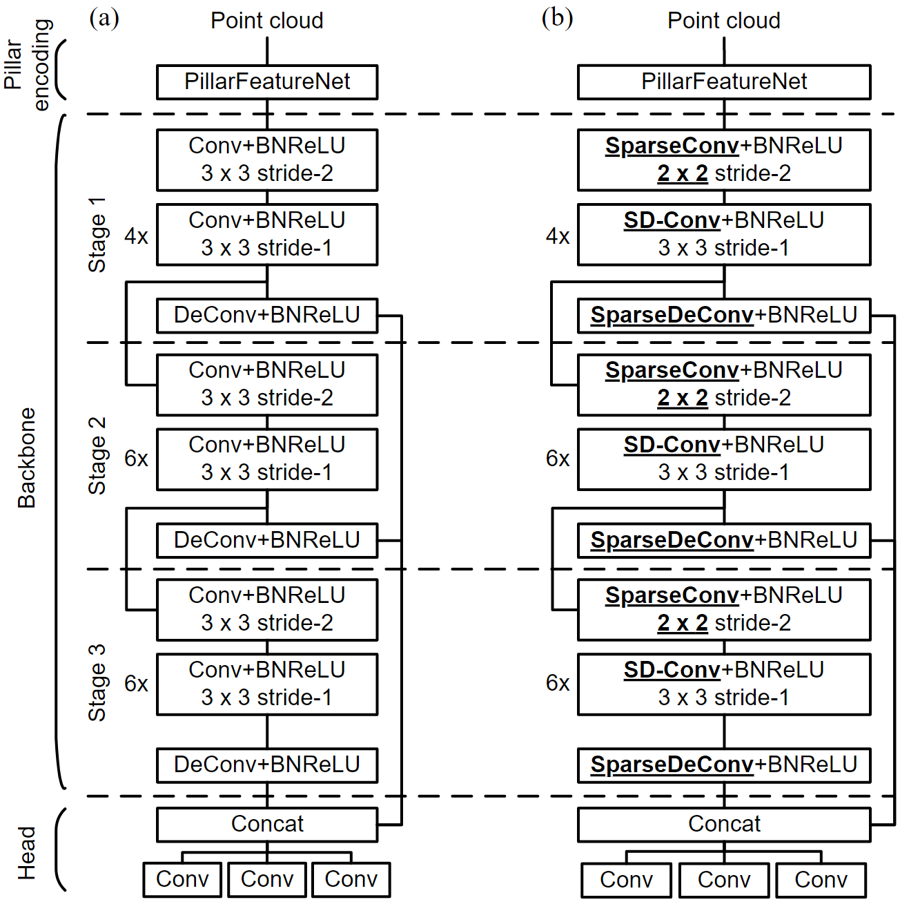
Figure 1: (a) Basic structure of PointPillars, (b) Applying SD-Conv in PointPillars.

For CenterPoint, as depicted in Fig. 2, it has the same backbone structure as PointPillars. However, its head structure differs as it adopts a multi-head architecture with individual heads assigned to each object type. In the model with SD-Conv applied, the CenterPoint backbone’s convolution operations are replaced with sparse convolution modules that include SD-Conv, similar to the approach in PointPillars.

As shown in Fig. 3, PillarNet has an advanced encoder structure for deep pillar feature extraction. Its backbone structure also diverges from PointPillars and CenterPoint. However, similar to CenterPoint, PillarNet’s head structure utilizes a multi-head approach. In the model where SD-Conv is employed, we replace Conv modules of backbone with a sparse convolution module that includes SD-Conv. This introduction of SD-Conv effectively reduces the backbone density by 27.05%, and brings down the overall FLOPs from 283.98G to 155.02G.

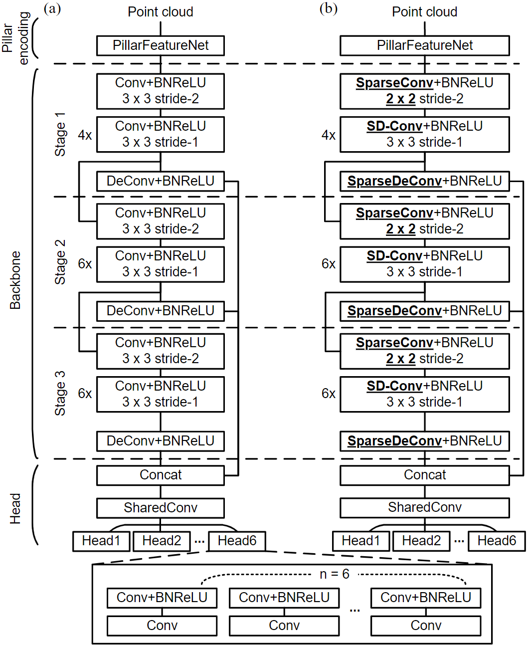
Figure 2: (a) Basic structure of CenterPoint, (b) Applying SD-Conv in CenterPoint.

Figure 3: (a) Basic structure of PillarNet, (b) Applying SD-Conv in PillarNet.

A.3 Applying Pruning from Scratch in Training: SDP-Conv

In terms of pruning, another consideration is the possibility of applying pruning from the beginning of the training process, a method we denote as SDP-Conv. The SDP-Conv module, utilizing both $I_{p}^{S\!P\!P}$ and $I_{p}^{S\!D}$, determines which pillars should be pruned and which should be subjected to dilate. This module is more general as it takes into account both pruning and dilation simultaneously. However, training with pruning applied from the scratch poses a challenge for achieving optimal learning. This is due to the removal of pillars before the feature extraction capabilities of the backbone network become sufficiently powerful, which results in a degradation in performance, as can be seen in Table 2.

Table 2: SD-Conv + SPP vs SDP on KITTI val set with PointPillars.

Method	FLOPs (G)	BEV			3D
		Easy	Mod	Hard	Easy	Mod	Hard
SD-Conv + SPP	4.46	90.29	87.63	85.45	87.44	77.22	75.08
SDP-Conv	4.64	90.00	87.34	84.45	86.88	76.99	74.59