Study of the semileptonic decays $\Upsilon(1S)\to B_{(c)}\ell\bar{\nu}_{\ell}$

Abstract

We study the exclusive semileptonic decays $\Upsilon(1S)\to B_{(c)}\ell\bar{\nu}_{\ell}$, where $\ell=e,\mu,\tau$. The relevant hadronic form factors are calculated using the Covariant Confined Quark Model developed previously by our group. We predict the branching fractions $\mathcal{B}(\Upsilon(1S)\to B_{(c)}\ell\bar{\nu}_{\ell})$ to be of the order of $10^{-13}$ and $10^{-10}$ for the case of $B$ and $B_{c}$, respectively. Our predictions agree well with other theoretical calculations. We also consider the effects of possible New Physics in the case of $\Upsilon(1S)\to B_{c}\tau\bar{\nu}_{\tau}$. We show that the branching fraction of this decay can be enhanced by an order of magnitude using the constraints from the $B\to D^{(*)}\ell\bar{\nu}_{\ell}$ and $B_{c}\to J/\psi\ell\bar{\nu}_{\ell}$ experimental data.

I   Introduction

Low-lying quarkonia systems such as $\Upsilon(1S)$ mostly decay through intermediate gluons or photons produced by the parent $\bar{q}q$ pair annialation. As a result, strong and radiative decays of $\Upsilon(1S)$ have been widely studied, both theoretically and experimentally. Meanwhile, weak decays of $\Upsilon(1S)$ have attracted less attention. Thank to the significant progress achieved in recent years in the improvement of luminosity of colliders, a large amount of rare weak decays have been observed. In particular, the rare semileptonic decay of the charmonium $J/\psi\to D\ell^{+}\nu_{\ell}$, ($\ell=e,\mu$), was considered one of the main research topics at BESIII experiment [1]. In 2021, BESIII reported a search for the decay $J/\psi\to De^{+}\nu_{e}$ based on a sample of $10.1\times 10^{9}$ $J/\psi$ events [2]. The result placed an upper limit of the branching fraction to be $\mathcal{B}(J/\psi\to De^{+}\nu_{e}+c.c.)<7.1\times 10^{-8}$ at 90 % confidence level (CL). It is worth mentioning that this upper limit was improved by a factor of 170 as compared to the previous one [3]. In 2023, using the same $J/\psi$ event sample, BESIII searched for the semimuonic channel for the first time and found un upper limit of $\mathcal{B}(J/\psi\to D\mu^{+}\nu_{\mu}+c.c.)<5.6\times 10^{-7}$ at 90 % CL [4]. These upper limits are still much larger than the Standard Model (SM) predictions, which are of order of $10^{-11}$ [5, 6, 7, 8, 9]. Nevertheless, the experimental data implied constraints on several New Physics models which can enhance the branching fractions to the order of $10^{-5}$ [10]. In the light of the extensive search for rare charmonium decays, it is reasonable to explore the similar decays of the bottomonium $\Upsilon(1S)$.

The semileptonic decays $\Upsilon(1S)\to B_{(c)}\ell\bar{\nu}_{\ell}$, where $\ell=e,\mu,\tau,$ have been investigated in several theoretical studies. However, there are so few of them. Besides, the existing predictions still differ. The first calculation of the decays $\Upsilon(1S)\to B_{c}\ell\bar{\nu}_{\ell}$ was carried out by Dhir, Verma, and Sharma [7] in the framework of the Bauer-Stech-Wirbel model. They obtained $\mathcal{B}(\Upsilon(1S)\to B_{c}e\bar{\nu}_{e})=1.70^{+0.03}_{-0.02}$ and $\mathcal{B}(\Upsilon(1S)\to B_{c}\tau\bar{\nu}_{\tau})=2.9^{+0.05}_{-0.02}$. In this paper, the authors only considered the $\Upsilon(1S)\to B_{c}$ transition. In 2017, Wang et al. calculated the decays $\Upsilon(1S)\to B^{(*)}_{(c)}\ell\bar{\nu}_{\ell}$ using the Bethe-Salpeter method [9]. The results for the $\Upsilon(1S)\to B_{c}$ case read $\mathcal{B}(\Upsilon(1S)\to B_{c}e\bar{\nu}_{e})=1.37^{+0.22}_{-0.19}$ and $\mathcal{B}(\Upsilon(1S)\to B_{c}\tau\bar{\nu}_{\tau})=4.17^{+0.58}_{-0.52}$. The results of the two studies above only marginally agree with each other. Let us now consider the ratio of branching fractions, namely, $R(\Upsilon(1S)\to B_{c})=\mathcal{B}(\Upsilon(1S)\to B_{c}\tau\bar{\nu}_{\tau}/\mathcal{B}(\Upsilon(1S)\to B_{c}e\bar{\nu}_{e})$. Based on the branching fractions given above, we estimate $R(\Upsilon(1S)\to B_{c})$ to be about $1.71\pm 0.06$ (Dhir et al.) and $3.04\pm 0.91$ (Wang et al.). The results imply a tension at $1.5~{}\sigma$ between the two studies. It is, therefore, necessary to provide more theoretical predictions for the decays.

There is another interesting aspect of the decay $\Upsilon(1S)\to B_{c}\ell\bar{\nu}_{\ell}$. At quark level, it is induced by the transition $b\to c\ell\bar{\nu}_{\ell}$. For more than a decade, tensions between experimental data and the Standard Model predictions for the ratios of branching fractions $R_{D}=\mathcal{B}(B^{0}\to D\tau\bar{\nu}_{\tau}/\mathcal{B}(B^{0}\to De\bar{\nu}_{e})$ and $R_{D^{*}}=\mathcal{B}(B^{0}\to D^{*}\tau\bar{\nu}_{\tau}/\mathcal{B}(B^{0}\to D^{*}e\bar{\nu}_{e})$ have never disappeared. It is well known in the community as “the $R_{D^{(*)}}$ puzzle”, which hints possible violation of lepton flavor universality (LFU) and motivates a huge search for New Physics in the semileptonic decays $B^{0}\to D^{(*)}\ell\bar{\nu}_{\ell}$ (see, e.g., [11, 12] and references therein). The decay $\Upsilon(1S)\to B_{c}\ell\bar{\nu}_{\ell}$ is therefore a reasonable candidate to probe possible New Physics beyond the SM.

Weak decays of hadrons such as $\Upsilon(1S)\to B_{(c)}\ell\bar{\nu}_{\ell}$ are characterized by the interplay of strong and weak interactions. While the structure of the weak interaction in semileptonic decays is well established, the strong interaction in the hadronic transitions $\Upsilon(1S)\to B_{(c)}$ can only be calculated using nonperturbative methods. Hadronic transitions are often parametrized by invariant form factors. In this paper, hadronic form factors of the semileptonic decays of $\Upsilon(1S)$ are calculated in the framework of the covariant confined quark model (CCQM) developed previously by our group. One of the advantages of our model is the ability to calculate the form factors in the whole physical range of transfered momentum without any extrapolation.

The rest of the paper is organized as follows. In Sec. II we present the relevant theoretical formalism for the calculation of the semileptonic decays $\Upsilon(1S)\to B_{(c)}\ell\bar{\nu}_{\ell}$. In Sec. III we briefly introduce the CCQM and demonstrate the calculation of the hadronic form factors in our model. We then present our numerical results in Sec. IV and conclude in Sec. V.

II   Formalism

In the CCQM the semileptonic decays $\Upsilon(1S)\to B_{(c)}\ell\bar{\nu}_{\ell}$ are described by the Feynman diagram in Fig. 1. The effective Hamiltonian for the semileptonic decays $\Upsilon(1S)\to B_{(c)}\ell\bar{\nu}_{\ell}$ is given by

$$\mathcal{H}_{\textrm{eff}}(b\to q\ell\bar{\nu}_{\ell})=\frac{G_{F}}{\sqrt{2}}V_{qb}\left[\bar{q}O^{\mu}b\right]\left[\bar{\ell}O_{\mu}\nu_{\ell}\right],$$ (1)

where $q=(u,c)$, $G_{F}$ is the Fermi constant, $V_{qb}$ is the Cabibbo-Kobayashi-Maskawa matrix element, and $O^{\mu}=\gamma^{\mu}(1-\gamma_{5})$ is the weak Dirac matrix with left chirality. The invariant matrix element of the decays is written as

$$\mathcal{M}(\Upsilon(1S)\to B_{(c)}\ell\bar{\nu}_{\ell})=\frac{G_{F}}{\sqrt{2}}V_{qb}\left\langle B_{(c)}|\bar{q}O^{\mu}b|\Upsilon(1S)\right\rangle\bar{\ell}O_{\mu}\nu_{\ell}.$$ (2)

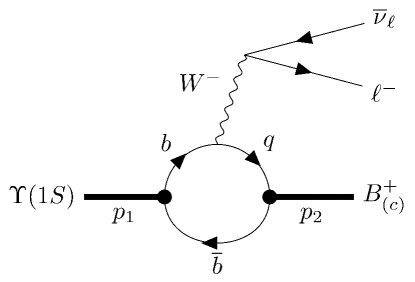
Figure 1: Feynman diagram for semileptonic decays $\Upsilon(1S)\to B_{(c)}\ell\bar{\nu}_{\ell}$.

The squared matrix element can be written as a product of the hadronic tensor $H_{\mu\nu}$ and leptonic tensor $L^{\mu\nu}$:

$$|\mathcal{M}|^{2}=\frac{G_{F}^{2}}{2}H_{\mu\nu}L^{\mu\nu}.$$ (3)

The leptonic tensor for the process $W^{-}_{\rm off-shell}\to\ell^{-}\bar{\nu}_{\ell}$ $\left(W^{+}_{\rm off-shell}\to\ell^{+}\nu_{\ell}\right)$ is given by [13]

$$L^{\mu\nu} = \left\{\begin{array}[]{lr}\mbox{\rm{tr}}\Big{[}(p\kern-5.0pt/_{\ell}+m_{\ell})O^{\mu}p\kern-5.0pt/_{\nu_{\ell}}O^{\nu}\Big{]}&\qquad\text{for}\qquad W^{-}_{\rm off-shell}\to\ell^{-}\bar{\nu}_{\ell}\\[5.16663pt] \mbox{\rm{tr}}\Big{[}(p\kern-5.0pt/_{\ell}-m_{\ell})O^{\nu}p\kern-5.0pt/_{\nu_{\ell}}O^{\mu}\Big{]}&\qquad\text{for}\qquad W^{+}_{\rm off-shell}\to\ell^{+}\nu_{\ell}\end{array}\right.$$ (6)

$$= 8\left(p_{\ell}^{\mu}p_{\nu_{\ell}}^{\nu}+p_{\ell}^{\nu}p_{\nu_{\ell}}^{\mu}-p_{\ell}\cdot p_{\nu_{\ell}}g^{\mu\nu}\pm i\varepsilon^{\mu\nu\alpha\beta}p_{\ell\alpha}p_{\nu_{\ell}\beta}\right),$$ (7)

where the upper/lower sign refers to the two $(\ell^{-}\bar{\nu}_{\ell})/(\ell^{+}\nu_{\ell})$ configurations. The sign change is due to the parity violating part of the lepton tensors. In our case we have to use the upper sign in Eq. (7).

The hadronic matrix element in Eq. (2) is often parametrized as a linear combination of Lorentz structures multiplied by scalar functions, namely, invariant form factors which depend on the momentum transfer squared. For the $V\to P$ transition one has

$$\langle B_{(c)}(p_{2})\left|\bar{q}O_{\mu}b\right|\Upsilon(1S)(\epsilon_{1},p_{1})\rangle\equiv\epsilon^{\alpha}_{1}T_{\mu\alpha}$$

$$=\frac{\epsilon_{1}^{\nu}}{m_{1}+m_{2}}[-g_{\mu\nu}pqA_{0}(q^{2})+p_{\mu}p_{\nu}A_{+}(q^{2})+q_{\mu}p_{\nu}A_{-}(q^{2})+i\varepsilon_{\mu\nu\alpha\beta}p^{\alpha}q^{\beta}V(q^{2})],$$ (8)

where $q=p_{1}-p_{2}$, $p=p_{1}+p_{2}$, $m_{1}=m_{\Upsilon(1S)}$, $m_{2}=m_{B_{(c)}}$, and $\epsilon_{1}$ is the polarization vector of $\Upsilon(1S)$, so that $\epsilon_{1}^{\dagger}\cdot p_{1}=0$. The particles are on-shell, i.e., $p_{1}^{2}=m_{1}^{2}=m^{2}_{\Upsilon(1S)}$ and $p_{2}^{2}=m_{2}^{2}=m^{2}_{B_{(c)}}$. The form factors $A_{0}(q^{2})$, $A_{\pm}(q^{2})$, and $V(q^{2})$ will be calculated later in our model. In terms of the invariant form factors, the hadronic tensor reads

$$H_{\mu\nu}=T^{VP}_{\mu\alpha}\left(-g^{\alpha\alpha^{\prime}}+\frac{p_{1}^{\alpha}p_{1}^{\alpha^{\prime}}}{m_{1}^{2}}\right)T^{VP\dagger}_{\nu\alpha^{\prime}},$$ (9)

where

$$T^{VP}_{\mu\alpha}=\frac{1}{m_{1}+m_{2}}\left[-g_{\mu\alpha}pqA_{0}(q^{2})+p_{\mu}p_{\alpha}A_{+}(q^{2})+q_{\mu}p_{\alpha}A_{-}(q^{2})+i\varepsilon_{\mu\alpha\gamma\delta}p^{\gamma}q^{\delta}V(q^{2})\right].$$ (10)

Finally, by summing up the vector polarizations, one obtains the decay width

$$\Gamma\left(\Upsilon(1S)\to B_{(c)}\ell\bar{\nu}_{\ell}\right)=\frac{G_{F}^{2}}{(2\pi)^{3}}\frac{|V_{qb}|^{2}}{64m_{1}^{3}}\int\limits_{m^{2}_{\ell}}^{(m_{1}-m_{2})^{2}}\!\!\!\!dq^{2}\int\limits_{s_{1}^{-}}^{s_{1}^{+}}\!\!ds_{1}\frac{1}{3}H_{\mu\nu}L^{\mu\nu},$$ (11)

where $m_{1}=m_{\Upsilon(1S)}$, $m_{2}=m_{B_{(c)}}$, and $s_{1}=(p_{B_{(c)}}+p_{\ell})^{2}$. The upper and lower bounds of $s_{1}$ are given by

$$s_{1}^{\pm}=m_{2}^{2}+m_{\ell}^{2}-\frac{1}{2q^{2}}\left[(q^{2}-m_{1}^{2}+m_{2}^{2})(q^{2}+m_{\ell}^{2})\mp\lambda^{1/2}(q^{2},m_{1}^{2},m_{2}^{2})\lambda^{1/2}(q^{2},m_{\ell}^{2},0)\right],$$ (12)

where $\lambda(x,y,z)\equiv x^{2}+y^{2}+z^{2}-2(xy+yz+zx)$ is the Källén function.

III   Form factors in the Covariant Confined Quark Model

III.1 CCQM in a nutshell

The CCQM has been developed for about three decades as a tool for hadronic calculation. It has been successfully employed to explore various decays of not only mesons and baryons, but also tetraquarks, pentaquarks, and other multiquark states. The model has been introduced in great details along the way in many studies by our group, for intance, Refs. [14, 15, 16]. We only list here the main features of the model for completeness, and also, to keep the text short and focus more on the new results.

The starting point of the CCQM is a Lagrangian describing the quark-hadron interaction with non-local characteristic. The Lagrangian has the following form for a meson $M$:

$$\mathcal{L}_{\mathrm{int}}(x)=g_{M}M(x)J(x)+\mathrm{H.c.},\qquad J(x)=\int dx_{1}\int dx_{2}F_{M}(x;x_{1},x_{2})[\bar{q}_{2}(x_{2})\Gamma_{M}q_{1}(x_{1})],$$ (13)

where $g_{M}$ is the meson-quark coupling constant, $\Gamma_{M}$ – the relevant Dirac matrix, $F_{M}(x;x_{1},x_{2})$–the vertex function whose form is chosen as follows

$$F_{M}(x;x_{1},x_{2})=\delta^{(4)}(x-\omega_{1}x_{1}-\omega_{2}x_{2})\Phi_{M}[(x_{1}-x_{2})^{2}].$$ (14)

Here, $\omega_{i}=m_{q_{i}}/(m_{q_{1}}+m_{q_{2}})$ with $m_{q_{i}}$ being the constituent quark mass. The function $\Phi_{M}[(x_{1}-x_{2})^{2}]$ is assumed to be Gaussian for simplicity, and is written in the momentum representation as

$$\widetilde{\Phi}_{M}(-p^{2})=\exp(p^{2}/\Lambda^{2}_{M}),$$ (15)

where $\Lambda_{M}$ is a parameter of the model.

The quark-meson coupling is obtained using the compositeness condition [17, 18]

$$Z_{M}=1-\Pi^{\prime}_{M}(m^{2}_{M})=0,$$ (16)

where $Z_{M}$ is the wave function renormalization constant of the meson $M$ and $\Pi^{\prime}_{M}$ is the derivative of the meson mass function.

Figure 2: One-loop self-energy diagram for a meson.

The meson mass function in Eq. (16) is defined by the Feynman diagram shown in Fig. 2 and has the following form:

$$\Pi_{P}(p) = 3g_{P}^{2}\int\!\!\frac{dk}{(2\pi)^{4}i}\,\widetilde{\Phi}^{2}_{P}\left(-k^{2}\right)\mbox{\rm{tr}}\left[S_{1}(k+w_{1}p)\gamma^{5}S_{2}(k-w_{2}p)\gamma^{5}\right],$$ (17)

$$\Pi_{V}(p) = g_{V}^{2}\left[g^{\mu\nu}-\frac{p^{\mu}p^{\nu}}{p^{2}}\right]\int\!\!\frac{dk}{(2\pi)^{4}i}\,\widetilde{\Phi}^{2}_{V}\left(-k^{2}\right)\mbox{\rm{tr}}\left[S_{1}(k+w_{1}p)\gamma_{\mu}S_{2}(k-w_{2}p)\gamma_{\nu}\right],$$ (18)

where

$$S_{i}(k)=\frac{1}{m_{q_{i}}-\not\!k-i\epsilon}=\frac{m_{q_{i}}+\not\!k}{m^{2}_{q_{i}}-k^{2}-i\epsilon}$$ (19)

is the quark propagator.

The CCQM has several free parameters including the constituent quark masses $m_{q}$, the hadron size parameters $\Lambda_{H}$, and a universal cutoff parameter $\lambda_{\mathrm{cutoff}}$ which guarantees the confinement of constituent quarks inside hadrons. These parameters are obtained by fitting to available experimental data and/or Lattice QCD. Once they are fixed, the CCQM can be used to calculate hadronic quantities in a straight-forward manner. The parameters relevant to this study are collected in Table 1.

Table 1: Quark masses, meson size parameters, and infrared cutoff parameter (all in GeV).

$m_{u/d}$	$m_{s}$	$m_{c}$	$m_{b}$	$\Lambda_{B}$	$\Lambda_{B_{c}}$	$\Lambda_{\Upsilon(1S)}$	$\lambda$
0.241	0.428	1.67	5.04	1.96	2.73	4.03	0.181

III.2 Hadronic matrix element and form factors

In the CCQM the hadronic matrix element of the semileptonic decays $\Upsilon(1S)\to B_{(c)}\ell\bar{\nu}_{\ell}$ is given by the diagram in Fig. 1 and is written as

$$\left\langle B_{(c)}(p_{2})\left|\bar{q}O_{\mu}b\right|\Upsilon(1S)(\epsilon_{1},p_{1})\right\rangle=\epsilon_{1}^{\alpha}T^{VP}_{\mu\alpha}$$

$$T^{VP}_{\mu\alpha} = 3g_{\Upsilon(1S)}g_{P}\int\!\!\frac{d^{4}k}{(2\pi)^{4}i}\widetilde{\Phi}_{\Upsilon(1S)}[-(k+w_{13}p_{1})^{2}]\widetilde{\Phi}_{P}[-(k+w_{23}p_{2})^{2}]$$ (20)

$$\times \mbox{\rm{tr}}\left[S_{2}(k+p_{2})O_{\mu}S_{1}(k+p_{1})\gamma_{\alpha}S_{3}(k)\gamma_{5}\right]$$

$$\equiv \frac{1}{m_{1}+m_{2}}\left[-g_{\mu\alpha}pqA_{0}(q^{2})+p_{\mu}p_{\alpha}A_{+}(q^{2})+q_{\mu}p_{\alpha}A_{-}(q^{2})+i\varepsilon_{\mu\alpha\gamma\delta}p^{\gamma}q^{\delta}V(q^{2})\right],$$

where $k$ is the loop momentum and $w_{ij}=m_{q_{j}}/(m_{q_{i}}+m_{q_{j}})$ $(i,j=1,2,3)$.

The form factors are then calculated using standard one-loop calculation techniques (see, e.g. Ref. [19]). The main steps are listed as follows. First, one substitutes the Gaussian form for the vertex functions in Eq. (15) into Eq. (20). Second, one uses the Fock-Schwinger representation for the quark propagator

$$S_{q_{i}}(k)=(m_{q_{i}}+\not\!k)\int\limits_{0}^{\infty}\!\!d\alpha_{i}\,e^{-\alpha_{i}(m_{q_{i}}^{2}-k^{2})}.$$ (21)

Third, one treats the integrals over the Fock-Schwinger parameters $0\leq\alpha_{i}<\infty$ by introducing an additional integration which converts the set of these parameters into a simplex as follows

$$\prod\limits_{i=1}^{n}\int\limits_{0}^{\infty}\!\!d\alpha_{i}f(\alpha_{1},\ldots,\alpha_{n})=\int\limits_{0}^{\infty}\!\!dtt^{n-1}\prod\limits_{i=1}^{n}\int\!\!d\alpha_{i}\delta\left(1-\sum\limits_{i=1}^{n}\alpha_{i}\right)f(t\alpha_{1},\ldots,t\alpha_{n}).$$ (22)

Note that Feynman diagrams are calculated in the Euclidean region where $p^{2}=-p^{2}_{E}$. The vertex functions fall off in the Euclidean region, therefore no ultraviolet divergence appears. In order to avoid possible thresholds in the Feynman diagram, we introduce a universal infrared cutoff which effectively guarantees the confinement of quarks within hadrons

$$\int\limits_{0}^{\infty}dt(\ldots)\to\int\limits_{0}^{1/\lambda^{2}}dt(\ldots).$$ (23)

Each form factor for the semileptonic transition $\Upsilon(1S)\to B_{(c)}$ is finally turned into a three-fold integrals of the general form

$$F(q^{2})=\int\limits_{0}^{1/\lambda^{2}}\!\!dtt^{2}\int\limits_{0}^{1}\!\!d\alpha_{1}\int\limits_{0}^{1-\alpha_{1}}\!\!d\alpha_{2}\,f(t\alpha_{1},t\alpha_{2}).$$ (24)

The expressions for $f(t\alpha_{1},t\alpha_{2})$ are obtained by a FORM code written by us. The numerical calculation of the three-fold integrals are done by using FORTRAN codes with the help of NAG library.

IV   Numerical results

Before listing our numerical results, we briefly discuss the estimation of the theoretical errors in our approach. It should be reminded that all phenomenological quark models of hadrons are simplied physics picture, and therefore it is very difficult to treat the theoretical error rigorously. The main source of uncertainties come from the free parameters in Table 1. They are obtained by a least-squares fit of leptonic and electromagnetic decay constants to experimental data and/or Lattice QCD. The allowed deviation in the fit is in the range 5–10%. This range can be used as reasonable estimation of the model’s errors. Moreover, the CCQM has been applied to study a broad range of hadron decay processes. We observed that our predictions often agree with experimental data within 10%. Therefore, we estimate the theoretical error of the predictions in this paper to be about 10%.

IV.1 Form factors

In Fig. 3 we present the form factors of the $\Upsilon(1S)\to B_{(c)}$ transitions in the full range of momentum transfer $0\leq q^{2}\leq q^{2}_{\rm max}=(m_{\Upsilon(1S)}-m_{B_{(c)}})^{2}$. It is worth mentioning that in the CCQM, the form factors are directly calculated in the whole physical range without any extrapolation as usually seen in Lattice QCD and QCD Sum Rules. We then parametrize the $q^{2}$ dependance of the form factors by using a general dipole approximation

$$F(q^{2})=\frac{F(0)}{1-as+bs^{2}},\quad s\equiv\frac{q^{2}}{m^{2}_{\Upsilon(1S)}}.$$ (25)

The dipole-approximation parameters for the $\Upsilon(1S)\to B_{(c)}$ form factors are displayed in Table 2. We also list here the values of the form factors at zero recoil, i.e., at $q^{2}_{\rm max}$. We compare the form factors at maximum recoil $(q^{2}=0)$ with other theoretical studies in Table 3.

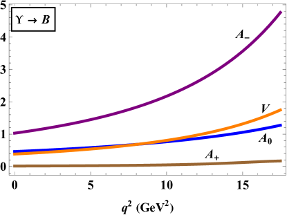
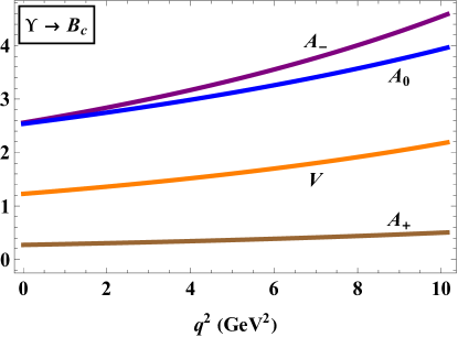
Figure 3: Our results for the form factors of the $\Upsilon(1S)\to B$ (left) and $\Upsilon(1S)\to B_{c}$ (right) transitions.

Table 2: Parameters of the dipole approximation for $\Upsilon(1S)\to B_{(c)}$ form factors and the form-factor values at zero recoil $q^{2}_{\rm max}$.

	$\Upsilon(1S)\to B$				$\Upsilon(1S)\to B_{c}$
	$A_{0}$	$A_{+}$	$A_{-}$	$V$	$A_{0}$	$A_{+}$	$A_{-}$	$V$
$F(0)$	0.46	0.013	1.03	0.38	2.54	0.27	2.56	1.23
$a$	3.93	8.99	5.64	5.63	3.49	4.91	4.57	4.54
$b$	3.41	21.9	8.34	8.37	2.83	7.43	5.93	5.89
$F(q^{2}_{\rm max})$	1.28	0.18	4.78	1.75	3.96	0.50	4.59	2.19

Table 3: Form factors at maximum recoil $q^{2}=0$ in the CCQM and other theoretical studies. The values in the row BS were estimated based the form-factor graphs of Ref. [9]

	$\Upsilon(1S)\to B$				$\Upsilon(1S)\to B_{c}$
	$A_{0}(0)$	$A_{+}(0)$	$A_{-}(0)$	$V(0)$	$A_{0}(0)$	$A_{+}(0)$	$A_{-}(0)$	$V(0)$
This work	0.46	0.013	1.03	0.38	2.54	0.27	2.56	1.23
BSW [7]					$3.06^{+0.10}_{-0.05}$	$0.38^{+0.06}_{-0.09}$		$1.61^{+0.01}_{-0.01}$
Ref. [20]					4.99	1.01		1.01
BS [9]	0.18	0.023	0.30	0.15	1.68	0.27	1.29	0.80

IV.2 Branching fractions

We present our results for the branching fractions of the semileptonic decays $\Upsilon(1S)\to B_{(c)}\ell\bar{\nu}_{\ell}$ ($\ell=e,\mu,\tau$) in Table 4. We also show in this table the relevant predictions of other theoretical studies for comparison. Our predictions agree well with the Bethe-Salpeter–approach results [9]. Regarding the results obtained using the Bauer-Stech-Wirbel model [7], the branching fractions for the electron and muon modes in this study agree with ours, but the one for the tau mode disagrees.

Table 4: Branching fractions of $\Upsilon(1S)$ semileptonic decays in the CCQM, the Bethe-Salpeter (BS) approach [9], and the Bauer-Stech-Wirbel (BSW) model [7].

Channel	Unit	This work	BS [9]	BSW [7]
$\Upsilon(1S)\to Be\bar{\nu}_{e}$	$10^{-13}$	5.96	$7.83^{+1.40}_{-1.20}$
$\Upsilon(1S)\to B\mu\bar{\nu}_{\mu}$	$10^{-13}$	5.95	$7.82^{+1.40}_{-1.20}$
$\Upsilon(1S)\to B\tau\bar{\nu}_{\tau}$	$10^{-13}$	3.30	$5.04^{+0.92}_{-0.79}$
$\Upsilon(1S)\to B_{c}e\bar{\nu}_{e}$	$10^{-10}$	1.84	$1.37^{+0.22}_{-0.19}$	$1.70^{+0.03}_{-0.02}$
$\Upsilon(1S)\to B_{c}\mu\bar{\nu}_{\mu}$	$10^{-10}$	1.83	$1.37^{+0.22}_{-0.19}$	$1.69^{+0.04}_{-0.02}$
$\Upsilon(1S)\to B_{c}\tau\bar{\nu}_{\tau}$	$10^{-11}$	4.74	$4.17^{+0.58}_{-0.52}$	$2.90^{+0.05}_{-0.02}$

It is interesting to consider the ratio $R_{B_{(c)}}\equiv\mathcal{B}(\Upsilon(1S)\to B_{(c)}\tau\bar{\nu}_{\tau}/\mathcal{B}(\Upsilon(1S)\to B_{(c)}\ell\bar{\nu}_{\ell})$, $(\ell=e,\mu)$, where a large part of theoretical and experimental uncertainties cancels. We list in (26) and (27) all available predictions for $R_{B_{(c)}}$ up till now:

$$R_{B}\equiv\frac{\mathcal{B}(\Upsilon(1S)\to B\tau\bar{\nu})}{\mathcal{B}(\Upsilon(1S)\to B\ell\bar{\nu})}=\left\{\begin{array}[]{lc}0.64&\qquad\text{{BS}~{}\cite[cite]{[\@@bibref{Number}{Wang:2016dkd}{}{}]}}\\ 0.55&\qquad\text{This work}\end{array}\right.,$$ (26)

$$R_{B_{c}}\equiv\frac{\mathcal{B}(\Upsilon(1S)\to B_{c}\tau\bar{\nu})}{\mathcal{B}(\Upsilon(1S)\to B_{c}\ell\bar{\nu})}=\left\{\begin{array}[]{lc}0.30&\qquad\text{{BS}~{}\cite[cite]{[\@@bibref{Number}{Wang:2016dkd}{}{}]}}\\ 0.17&\qquad\text{{BSW}~{}\cite[cite]{[\@@bibref{Number}{Dhir:2009rb}{}{}]}}\\ 0.26&\qquad\text{This work}\end{array}\right..$$ (27)

Our results for the ratios $R_{B}$ and $R_{B_{c}}$ agree well with those in the BS approach. Meanwhile, the result for $R_{B_{c}}$ in the BSW is about two times smaller than the BS and our predictions. Therefore, we propose that the value $R_{B_{c}}\simeq 0.3$ is a reliable prediction.

IV.3 $\Upsilon(1S)\to B_{c}\ell\bar{\nu}_{\ell}$ beyond the Standard Model

As already mentioned in Sec. I, the semileptonic decay $\Upsilon(1S)\to B_{c}\ell\bar{\nu}_{\ell}$ is induced by the quark-level transition $b\to c\ell\bar{\nu}_{\ell}$ and can be linked with the $R_{D}^{(*)}$ anomaly. It is therefore interesting to probe the possible New Physics (NP) effects in the $\Upsilon(1S)$ semitauonic decay. Based on the current status of the anomalies, we assume that NP only affects leptons of the third generation and modify the effective Hamiltonian for the quark-level transition $b\to c\tau^{-}\bar{\nu}_{\tau}$ as follows

$${\mathcal{H}}_{eff} = 2\sqrt{2}G_{F}V_{cb}[(1+V_{L})\mathcal{O}_{V_{L}}+V_{R}\mathcal{O}_{V_{R}}],$$ (28)

where the four-fermion operators are written as

$$\mathcal{O}_{V_{L}}=\left(\bar{c}\gamma^{\mu}P_{L}b\right)\left(\bar{\tau}\gamma_{\mu}P_{L}\nu_{\tau}\right),$$

$$\mathcal{O}_{V_{R}}=\left(\bar{c}\gamma^{\mu}P_{R}b\right)\left(\bar{\tau}\gamma_{\mu}P_{L}\nu_{\tau}\right).$$ (29)

Here, $P_{L,R}=(1\mp\gamma_{5})/2$ are the left and right projection operators, and $V_{L,R}$ are the complex Wilson coefficients governing the NP contributions. In the SM one has $V_{L,R}=0$.

The invariant matrix element of the semileptonic decay $\Upsilon(1S)\to B_{c}\tau\bar{\nu}_{\tau}$ is then written as

$$\mathcal{M}|_{\rm NP} = \frac{G_{F}V_{cb}}{\sqrt{2}}\Big{[}(1+V_{R}+V_{L})\langle B_{c}|\bar{c}\gamma^{\mu}b|\Upsilon(1S)\rangle\bar{\tau}\gamma_{\mu}(1-\gamma^{5})\nu_{\tau}$$ (30)

$$+(V_{R}-V_{L})\langle B_{c}|\bar{c}\gamma^{\mu}\gamma^{5}b|\Upsilon(1S)\rangle\bar{\tau}\gamma_{\mu}(1-\gamma^{5})\nu_{\tau}\Big{]}.$$

Note that the axial hadronic currents do not contribute to the $P\to P^{\prime}$ transition. Therefore, assuming that NP appears in both $\bar{B}^{0}\to D$ and $\bar{B}^{0}\to D^{*}$ transitions, the case of pure $V_{R}-V_{L}$ coupling is ruled out. The branching fraction $\mathcal{B}(\Upsilon(1S)\to B_{c}\tau\bar{\nu}_{\tau})$ is therefore modified according to

$$\mathcal{B}(\Upsilon(1S)\to B_{c}\tau\bar{\nu}_{\tau})|_{\rm NP}=|1+V_{L}+V_{R}|^{2}\mathcal{B}(\Upsilon(1S)\to B_{c}\tau\bar{\nu}_{\tau})|_{\rm SM}.$$ (31)

By assumming the dominance of only one NP operator at a time, the allowed regions for the NP Wilson coefficients $V_{L(R)}$ are obtained using experimental data for the ratios of branching fractions $R_{D}=0.344\pm 0.026$, $R_{D^{*}}=0.285\pm 0.012$ [21], $R_{J/\psi}=0.71\pm 0.17\pm 0.18$ [22], the upper limit ${\cal B}(B_{c}\to\tau\nu)\leq 10\,\%$ from the LEP1 data [23], and the longitudinal polarization fraction of the $D^{*}$ meson $F_{L}^{D^{*}}({B}\to D^{\ast}\tau\bar{\nu}_{\tau})=0.43\pm 0.06\pm 0.03$ [24]. The relevant form factors for the transitions $B\to D^{(*)}$ and $B_{c}\to J/\psi$ were calculated in our paper [25]. In Fig. 4, we show the allowed regions for $V_{L}$ and $V_{R}$ within $2\sigma$. In each region, we find a best-fit value and mark it with an asterisk.

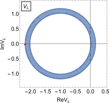
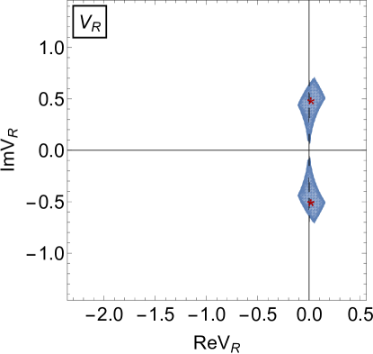
Figure 4: Constraints on the complex Wilson coefficients $V_{L}$ and $V_{R}$ from the measurements of $R_{D}$, $R_{D^{*}}$, $R_{J/\psi}$, and $F_{L}^{D^{*}}({B}\to D^{\ast}\tau\nu_{\tau})$ within $2\sigma$, and from the branching fraction ${\cal B}(B_{c}\to\tau\nu_{\tau})\leq 10\%$. The allowed regions are indicated in light-blue color. The asterisk symbols indicate the best-fit values.

We summarize our predictions for the branching fraction $\mathcal{B}(\Upsilon(1S)\to B_{c}\tau\bar{\nu}_{\tau})$ and the ratio of branching fractions $R_{B_{c}}$ in Table 5. The row labeled by SM (CCQM) contains our predictions within the SM with the CCQM form factors. The predicted intervals for the observables in the presence of NP are given in correspondence with the $2\sigma$ allowed regions of the NP Wilson coefficients depicted in Fig. 4. It is worth mentioning that the $V_{L}$ NP scenario can enhance the physical observables by a factor of 6.

Table 5: Observables in the SM and in the presence of NP.

Quantity	SM (CCQM)	$V_{R}$	$V_{L}$
$10^{11}\times\mathcal{B}(\Upsilon(1S)\to B_{c}\tau\bar{\nu}_{\tau})$	4.74	$(4.77,7.07)$	$(4.74,27.3)$
$R_{B_{c}}$	0.26	$(0.26,0.39)$	$(0.26,1.50)$

V   Summary

This paper represents a new study of the semileptonic decays $\Upsilon(1S)\to B_{(c)}\ell\bar{\nu}_{\ell}$, where $\ell=e,\mu,\tau,$ inspired by the recent search for similar rare weak decays of $J/\psi$ at BESIII. The relevant form factors for the $\Upsilon(1S)\to B_{(c)}$ transitions are calculated in the whole momentum transfer squared region in the framework of the Covariant Confined Quark Model. Predictions for the branching fractions and their ratios are reported and compared to other theoretical studies. A good agreement with the results of the Bethe-Salpeter approach was found. However, our prediction for the ratio of branching fractions $R_{B_{(c)}}\equiv\mathcal{B}(\Upsilon(1S)\to B_{(c)}\tau\bar{\nu}_{\tau}/\mathcal{B}(\Upsilon(1S)\to B_{(c)}\ell\bar{\nu}_{\ell})$ disagrees with the Bauer-Stech-Wirbel model prediction. We predict $R_{B_{c}}=0.26$ and $R_{B}=0.55$ which are close to the values $R_{B_{c}}=0.30$ and and $R_{B}=0.64$ obtained in the Bethe-Salpeter approach. We also extend the SM effective Hamiltonian for the $b\to c\tau\bar{\nu}_{\tau}$ transition by including left- and right-handed 4-fermion operators of dimension six. The relevant Wilson coefficients are obtained based on experimental data. Using the $2\sigma$ allowed regions for these coefficients, we found that the branching fraction of the tau mode as well as the ratio $R_{B_{c}}$ can be enhanced by about an order of magnitude. There have been only few theoretical calculations for $\Upsilon(1S)$ semileptonic decays to date. This study therefore provides more insights for experimental test of the SM, as well as the search for NP at future colliders.

- [1] M. Ablikim et al. [BESIII], Future Physics Programme of BESIII, Chin. Phys. C 44, no.4, 040001 (2020) [arXiv:1912.05983].
- [2] M. Ablikim et al. [BESIII], Search for the rare semi-leptonic decay , JHEP 06, 157 (2021) [arXiv:2104.06628].
- [3] M. Ablikim et al. [BES], Search for the rare decays , , and , Phys. Lett. B 639, 418-423 (2006) [arXiv:hep-ex/0604005].
- [4] M. Ablikim et al. [BESIII], Search for the semi-muonic charmonium decay , JHEP 01, 126 (2024) [arXiv:2307.02165].
- [5] Y. M. Wang, H. Zou, Z. T. Wei, X. Q. Li and C. D. Lü, The Transition form-factors for semi-leptonic weak decays of in QCD sum rules, Eur. Phys. J. C 54, 107-121 (2008) [arXiv:0707.1138].
- [6] Y. L. Shen and Y. M. Wang, weak decays in the covariant light-front quark model, Phys. Rev. D 78, 074012 (2008)
- [7] R. Dhir, R. C. Verma, and A. Sharma Effects of Flavor Dependence on Weak Decays of and , Adv. High Energy Phys. 2013, 706543 (2013) [arXiv:0903.1201].
- [8] M. A. Ivanov and C. T. Tran, Exclusive decays in a covariant constituent quark model with infrared confinement, Phys. Rev. D 92, 074030 (2015) [arXiv:1701.07377].
- [9] T. Wang, Y. Jiang, H. Yuan, K. Chai, and G. L. Wang, Weak decays of and , J. Phys. G 44, no.4, 045004 (2017) [arXiv:1604.03298].
- [10] A. Datta, P. J. O’Donnell, S. Pakvasa and X. Zhang, Flavor changing processes in quarkonium decays, Phys. Rev. D 60, 014011 (1999) [arXiv:hep-ph/9812325].
- [11] S. Groote, M. A. Ivanov, J. G. Körner, V. E. Lyubovitskij, P. Santorelli and C. T. Tran, Form-factor-independent test of lepton universality in semileptonic heavy meson and baryon decays, Phys. Rev. D 103, 093001 (2021) [arXiv:2102.12818].
- [12] M. A. Ivanov, J. G. Körner, P. Santorelli and C. T. Tran, Polarization as an Additional Constraint on New Physics in the Transition, Particles 3, no.1, 193-207 (2020) [arXiv:2009.00306].
- [13] T. Gutsche, M. A. Ivanov, J. G. Körner, V. E. Lyubovitskij, P. Santorelli, and N. Habyl, Semileptonic decay Phys. Rev. D 91, 074001 (2015); 91, 119907(E) (2015) [arXiv:1502.04864].
- [14] T. Branz, A. Faessler, T. Gutsche, M. A. Ivanov, J. G. Körner and V. E. Lyubovitskij, Relativistic constituent quark model with infrared confinement, Phys. Rev. D 81, 034010 (2010) [arXiv:0912.3710].
- [15] M. A. Ivanov, J. G. Körner, and P. Santorelli, Exclusive semileptonic and nonleptonic decays of the meson, Phys. Rev. D 73, 054024 (2006) [arXiv:hep-ph/0602050].
- [16] C. T. Tran, M. A. Ivanov, P. Santorelli, and Q. C. Vo, Radiative decays in covariant confined quark model, Chin. Phys. C 48, no.2, 023103 (2024) [arXiv:2311.15248].
- [17] A. Salam, Lagrangian Theory Of Composite Particles, Nuovo Cim. 25, 224 (1962).
- [18] S. Weinberg, Elementary Particle Theory Of Composite Particles, Phys. Rev. 130, 776 (1963).
- [19] M. A. Ivanov, J. G. Körner and C. T. Tran, Exclusive decays and in the covariant quark model, Phys. Rev. D 92, 114022 (2015) [arXiv:1508.02678].
- [20] K. K. Sharma and R. C. Verma, Rare decays of psi and upsilon, Int. J. Mod. Phys. A 14, 937 (1999) [hep-ph/9801202].
- [21] Y. S. Amhis et al. [HFLAV], Averages of b-hadron, c-hadron, and -lepton properties as of 2021,” Phys. Rev. D 107, 052008 (2023) [arXiv:2206.07501].
- [22] R. Aaij et al. [LHCb], Measurement of the ratio of branching fractions /, Phys. Rev. Lett. 120, 121801 (2018) [arXiv:1711.05623].
- [23] A. G. Akeroyd and C. H. Chen, Constraint on the branching ratio of from LEP1 and consequences for anomaly, Phys. Rev. D 96, 075011 (2017) [arXiv:1708.04072].
- [24] R. Aaij et al. [LHCb], Measurement of the longitudinal polarization in decays, [arXiv:2311.05224].
- [25] C. T. Tran, M. A. Ivanov, J. G. Körner and P. Santorelli, Implications of new physics in the decays , Phys. Rev. D 97, 054014 (2018) [arXiv:1801.06927].