Lecture Notes on Linear Neural Networks:
A Tale of Optimization and Generalization in Deep Learning

Abstract

These notes are based on a lecture delivered by NC on March 2021, as part of an advanced course in Princeton University on the mathematical understanding of deep learning. They present a theory (developed by NC, NR and collaborators) of linear neural networks — a fundamental model in the study of optimization and generalization in deep learning. Practical applications born from the presented theory are also discussed. The theory is based on mathematical tools that are dynamical in nature. It showcases the potential of such tools to push the envelope of our understanding of optimization and generalization in deep learning. The text assumes familiarity with the basics of statistical learning theory. Exercises (without solutions) are included.

1 Introduction

Deep learning (machine learning with neural network models subject to gradient-based training) is delivering groundbreaking performance, which facilitates the rise of artificial intelligence (see LeCun et al. (2015)). However, despite its extreme popularity, our formal understanding of deep learning is limited. Its application in practice is based primarily on conventional wisdom, trial-and-error and intuition, often leading to suboptimal results (compromising not only effectiveness, but also safety, robustness, privacy, fairness and more). Consequently, immense interest in developing mathematical theories behind deep learning has arisen, in the hopes that such theories will shed light on existing empirical findings, and more importantly, lead to principled methods that bring forth improved performance and new capabilities.

From the perspective of statistical learning theory, understanding deep learning requires addressing three fundamental questions: expressiveness, optimization and generalization. Expressiveness refers to the ability of compactly sized neural networks to represent functions capable of solving real-world problems. Optimization concerns the effectiveness of simple gradient-based algorithms in solving neural network training programs that are non-convex and thus seemingly difficult. Generalization treats the phenomenon of neural networks not overfitting even when having much more trainable parameters (weights) than examples to train on.

In these lecture notes we theoretically analyze linear neural networks — a fundamental model in the study of optimization and generalization in deep learning. A linear neural network is a feed-forward fully-connected neural network with linear (no) activation. Namely, for depth $n\in{\mathbb{N}}_{\geq 2}$, input dimension $d_{0}\in{\mathbb{N}}$, output dimension $d_{n}\in{\mathbb{N}}$, and hidden dimensions $d_{1},d_{2},\ldots,d_{n-1}\in{\mathbb{N}}$, it refers to the parametric family of hypotheses $\{{\mathbf{x}}\mapsto W_{n}W_{n-1}\cdots W_{1}{\mathbf{x}}:W_{j}\in{\mathbb{R}}^{d_{j}\times d_{j-1}},j=1,2,\ldots,n\}$, where $W_{j}$ is regarded as the weight matrix of layer $j$. Linear neural networks are trivial from the perspective of expressiveness (they realize only linear input-output mappings), but not so in terms of optimization and generalization — they lead to highly non-convex training objectives with multiple minima and saddle points, and when applied to underdetermined learning problems (e.g. matrix sensing; see Subsection 4.1 below) it is unclear a priori what kind of solutions gradient-based algorithms will converge to. By virtue of these properties, linear neural networks often serve as a theoretical surrogate for practical deep learning, allowing for controlled analyses of optimization and generalization (see, e.g., Baldi and Hornik (1989); Fukumizu (1998); Saxe et al. (2014); Kawaguchi (2016); Hardt and Ma (2016); Ge et al. (2016); Gunasekar et al. (2017); Li et al. (2018); Du et al. (2018); Nar and Sastry (2018); Bartlett et al. (2018); Laurent and Brecht (2018); Arora et al. (2018; 2019a; 2019b); Du and Hu (2019); Lampinen and Ganguli (2019); Ji and Telgarsky (2019); Gidel et al. (2019); Wu et al. (2019); Eftekhari (2020); Mulayoff and Michaeli (2020); Razin and Cohen (2020); Advani et al. (2020); Chou et al. (2020); Li et al. (2021); Yun et al. (2021); Min et al. (2021); Tarmoun et al. (2021); Azulay et al. (2021); Nguegnang et al. (2021); Bah et al. (2021)). The theory presented in these notes is dynamical in nature, i.e. relies on careful characterizations of the trajectories assumed in training. It will demonstrate the potential of dynamical techniques to succeed where other theoretical approaches fail.

Throughout the text, we consider the case where a linear neural network can express any linear (input-output) mapping, meaning that its hidden dimensions are large enough to not constrain rank, i.e. $d_{j}\geq\min\{d_{0},d_{n}\}$ for $j=1,2,\ldots,n-1$. Many of the presented results will not rely on this assumption, but for simplicity it is maintained throughout.

2 Dynamical Analysis

Suppose we are given an analytic training loss $\ell:{\mathbb{R}}^{d_{n}\times d_{0}}\to{\mathbb{R}}$ defined over linear mappings from ${\mathbb{R}}^{d_{0}}$ to ${\mathbb{R}}^{d_{n}}$. For example, $\ell(\cdot)$ could correspond to a linear regression task with $d_{0}$ input variables and $d_{n}$ output variables, or a multinomial logistic regression task with instances in ${\mathbb{R}}^{d_{0}}$ and $d_{n}$ possible labels. In line with these examples we typically think of $\ell(\cdot)$ as being convex, though unless stated otherwise this will not be assumed. Applying a linear neural network to $\ell(\cdot)$ boils down to optimizing the overparameterized objective:

$$\phi:{\mathbb{R}}^{d_{1}\times d_{0}}\times{\mathbb{R}}^{d_{2}\times d_{1}}\times\cdots\times{\mathbb{R}}^{d_{n}\times d_{n-1}}\to{\mathbb{R}}\text{\,,}$$ (1)

$$\phi(W_{1},W_{2},\ldots,W_{n})=\ell(W_{n}W_{n-1}\cdots W_{1})\text{\,.}$$

While the loss $\ell(\cdot)$ may be convex, the following proposition shows that, aside from degenerate cases (namely, aside from cases where $\ell(\cdot)$ is globally minimized by the zero mapping), the overparameterized objective $\phi(\cdot)$ is non-convex.

Proposition 1.

If $\ell(\cdot)$ does not attain its global minimum at the origin then $\phi(\cdot)$ is non-convex.

Proof.

If $\ell(\cdot)$ does not attain its global minimum at the origin then the same applies to $\phi(\cdot)$. This means that if $\phi(\cdot)$ is convex, its gradient at the origin must be non-zero. However, the latter gradient is clearly zero. ∎

We are interested in the dynamics of gradient-based optimization when applied to the overparameterized objective $\phi(\cdot)$. Our analysis will focus on gradient flow — a continuous version of gradient descent (attained by taking the step size to be infinitesimal). Under gradient flow, each weight matrix $W_{j}$ traverses through a continuous curve, which (with slight overloading of notation) we denote by $W_{j}(\cdot)$. Accordingly, $W_{j}(0)$ represents the value of $W_{j}$ at initialization, and $W_{j}(t)$ its value at time $t\in{\mathbb{R}}_{>0}$ of optimization. With a chosen initialization $W_{1}(0),W_{2}(0),\ldots,W_{n}(0)$, the curves $W_{1}(\cdot),W_{2}(\cdot),\ldots,W_{n}(\cdot)$ are defined through the following set of differential equations:

$$\dot{W}_{j}(t):=\tfrac{d}{dt}W_{j}(t)=-\tfrac{\partial}{\partial W_{j}}\,\phi(W_{1}(t),W_{2}(t),\ldots,W_{n}(t))\text{\,,}~{}~{}t>0~{},~{}j=1,2,\ldots,n\text{\,.}$$ (2)

We note that it is possible to translate to gradient descent (with positive step size) many of the gradient flow results which will be derived, either through analogous discrete analyses (see, e.g., Arora et al. (2019a)), or by bounding the distance between gradient descent and gradient flow (see Elkabetz and Cohen (2021)).

Moving on to our dynamical analysis, the first observation we make is that optimization conserves certain quantities.

Lemma 1.

For each $j=1,2,\ldots,n-1$, the curve $W_{j+1}^{\top}(\cdot)W_{j+1}(\cdot)-W_{j}(\cdot)W_{j}^{\top}(\cdot)$ is constant through time, i.e. $W_{j+1}^{\top}(t)W_{j+1}(t)-W_{j}(t)W_{j}^{\top}(t)=W_{j+1}^{\top}(0)W_{j+1}(0)-W_{j}(0)W_{j}^{\top}(0)$ for all $t>0$.

Proof.

A straightforward derivation shows that:

$$\tfrac{\partial}{\partial W_{j}}\,\phi(W_{1}(t),W_{2}(t),\ldots,W_{n}(t))=W_{n:j+1}^{\top}(t)\nabla\ell(W_{n:1}(t))W_{j-1:1}^{\top}(t)\text{\,,}~{}~{}t>0~{},~{}j=1,2,\ldots,n\text{\,,}$$

where $W_{n:j+1}(t):=W_{n}(t)W_{n-1}(t)\cdots W_{j+1}(t)$ and $W_{j-1:1}(t):=W_{j-1}(t)W_{j-2}(t)\cdots W_{1}(t)$ for all $j=1,2,\ldots,n$ (by convention, $W_{n:n+1}(t)$ and $W_{0:1}(t)$ stand for identity matrices). Under gradient flow (Equation (2)) we therefore have that:

$$W_{j+1}^{\top}(t)\dot{W}_{j+1}(t)=\dot{W}_{j}(t)W_{j}^{\top}(t)\text{\,,}~{}~{}t>0~{},~{}j=1,2,\ldots,n-1\text{\,.}$$

For $t>0$ and $j=1,2,\ldots,n-1$, adding the transpose of the equation above to itself gives:

$$W_{j+1}^{\top}(t)\dot{W}_{j+1}(t)+\dot{W}_{j+1}^{\top}(t)W_{j+1}(t)=W_{j}(t)\dot{W}_{j}^{\top}(t)+\dot{W}_{j}(t)W_{j}^{\top}(t)\text{\,.}$$

Notice that the left hand side is simply $\tfrac{d}{dt}(W_{j+1}^{\top}(t)W_{j+1}(t))$ while the right hand side is $\tfrac{d}{dt}(W_{j}(t)W_{j}^{\top}(t))$. Hence, integrating with respect to time leads to:

$$W_{j+1}^{\top}(t)W_{j+1}(t)-W_{j+1}^{\top}(0)W_{j+1}(0)=W_{j}(t)W_{j}^{\top}(t)-W_{j}(0)W_{j}^{\top}(0)\text{\,.}$$

Rearranging the equality completes the proof. ∎

If the constant matrix to which $W_{j+1}^{\top}(\cdot)W_{j+1}(\cdot)-W_{j}(\cdot)W_{j}^{\top}(\cdot)$ equals is zero, then for every $t>0$ the matrices $W_{j}(t)$ and $W_{j+1}(t)$ admit a certain “balancedness” (e.g., the non-zero singular values of $W_{j}(t)$ coincide with those of $W_{j+1}(t)$). We accordingly make the following definition.

Definition 1.

The unbalancedness magnitude of the weight matrices $W_{1},W_{2},\ldots,W_{n}$ is defined to be:

$$\max\nolimits_{j=1,2,\ldots,n-1}\|W_{j+1}^{\top}W_{j+1}-W_{j}W_{j}^{\top}\|_{F}\text{\,,}$$

where $\|\cdot\|_{F}$ stands for Frobenius norm.

With Definition 1 in place, Lemma 1 implies that the unbalancedness magnitude is conserved throughout optimization.

Proposition 2.

For every $t>0$, the unbalancedness magnitude of $W_{1}(t),W_{2}(t),\ldots,W_{n}(t)$ is equal to that of $W_{1}(0),W_{2}(0),\ldots,W_{n}(0)$.

Proof.

The result follows immediately from Lemma 1 and the definition of unbalancedness magnitude (Definition 1). ∎

In deep learning, the way that optimization is initialized has vital importance (see Sutskever et al. (2013)). It is common practice to initialize near zero, and we accordingly direct our attention to this regime. In our context, near-zero initialization implies that unbalancedness magnitude is small when optimization commences. By Proposition 2, this means that it will stay small throughout, and in particular, as optimization moves away from the origin, the unbalancedness magnitude becomes smaller and smaller relative to the weight matrices. We will make an idealized assumption of unbalancedness magnitude zero.

Assumption 1.

$W_{1}(0),W_{2}(0),\ldots,W_{n}(0)$ — the weight matrices at initialization — have unbalancedness magnitude zero.

Note that Assumption 1 does not limit the expressiveness of the linear neural network, since any linear mapping can be expressed by a product of weight matrices with unbalancedness magnitude zero (see Procedure 1 in Arora et al. (2019a)). It is possible to extend results derived for unbalancedness magnitude zero to the more general case of small unbalancedness magnitude (see, e.g., Razin and Cohen (2020)), but for simplicity this will not be demonstrated.

The following definition will serve for reasoning about the dynamics of the input-output mapping realized by the network.

Definition 2.

The end-to-end matrix corresponding to the weight matrices $W_{1},W_{2},\ldots,W_{n}$ is:

$$W_{n:1}:=W_{n}W_{n-1}\cdots W_{1}\text{\,.}$$

In accordance with Definition 2, we denote by $W_{n:1}(\cdot)$ the curve traversed by the end-to-end matrix during optimization, i.e. $W_{n:1}(\cdot):=W_{n}(\cdot)W_{n-1}(\cdot)\cdots W_{1}(\cdot)$. At the heart of our dynamical analysis lies Theorem 1 below, which characterizes the dynamics of $W_{n:1}(\cdot)$.

Theorem 1 (end-to-end dynamics).

It holds that:

$$\dot{W}_{n:1}(t):=\tfrac{d}{dt}W_{n:1}(t)=-\sum\nolimits_{j=1}^{n}\left[W_{n:1}(t)W_{n:1}^{\top}(t)\right]^{\frac{j-1}{n}}\nabla\ell\big{(}W_{n:1}(t)\big{)}\left[W_{n:1}^{\top}(t)W_{n:1}(t)\right]^{\frac{n-j}{n}}~{}~{},~{}t>0\text{\,,}$$ (3)

where $[\,\cdot\,]^{\beta}$, $\beta\in{\mathbb{R}}_{\geq 0}$, stands for a power operator defined over positive semidefinite matrices (with $\beta=0$ yielding identity by definition).

Proof.

For simplicity, we assume that all weight matrices are square, i.e. there exists $d\in{\mathbb{N}}$ such that $d=d_{0}=d_{1}=\cdots=d_{n}$. This assumption can be avoided at the expense of slightly more involved derivations that take into account possible differences in the dimensions. Below, for $j=1,2,\ldots,n$ we denote $W_{n:j+1}(t):=W_{n}(t)W_{n-1}(t)\cdots W_{j+1}(t)$ and $W_{j-1:1}(t):=W_{j-1}(t)W_{j-2}(t)\cdots W_{1}(t)$ (by convention, $W_{n:n+1}(t)$ and $W_{0:1}(t)$ stand for identity matrices).

Differentiating $W_{n:1}(t)$ with respect to time using the product rule gives:

$$\begin{split}\dot{W}_{n:1}(t)&=\sum\nolimits_{j=1}^{n}W_{n:j+1}(t)\dot{W}_{j}(t)W_{j-1:1}(t)\\ &=-\sum\nolimits_{j=1}^{n}W_{n:j+1}(t)W_{n:j+1}^{\top}(t)\nabla\ell(W_{n:1}(t))W_{j-1:1}^{\top}(t)W_{j-1:1}(t)\text{\,,}\end{split}$$ (4)

where the second equality is due to the fact that under gradient flow

$$\begin{split}\dot{W}_{j}(t)&:=-\tfrac{\partial}{\partial W_{j}}\,\phi(W_{1}(t),W_{2}(t),\ldots,W_{n}(t))\\ &=-W_{n:j+1}^{\top}(t)\nabla\ell(W_{n:1}(t))W_{j-1:1}^{\top}(t)\text{\,,}~{}~{}t>0~{},~{}j=1,2,\ldots,n\text{\,.}\end{split}$$

Now, by Assumption 1 and Proposition 2, the unbalancedness magnitude of $W_{1}(t),W_{2}(t),\ldots,W_{n}(t)$ is zero for all $t\geq 0$. Consequently:

$$W_{j+1}^{\top}(t)W_{j+1}(t)=W_{j}(t)W_{j}^{\top}(t)\text{\,,}~{}~{}t>0~{},~{}j=1,2,\ldots,n-1\text{\,.}$$ (5)

Fixing some $t>0$, we construct singular value decompositions for $W_{1}(t),W_{2}(t),\ldots,W_{n}(t)$ in an iterative process as follows. First, let $W_{1}(t)=U_{1}S_{1}V_{1}^{\top}$ be an arbitrary singular value decomposition of $W_{1}(t)$, i.e.  $U_{1},V_{1}\in{\mathbb{R}}^{d\times d}$ are orthogonal matrices and $S_{1}\in{\mathbb{R}}^{d\times d}$ is diagonal holding the singular values of $W_{1}(t)$. Then, for $j=2,3,\ldots,n$, notice that any left singular vector ${\mathbf{u}}$ of $W_{j-1}(t)$ with corresponding singular value $\sigma$ is an eigenvector of $W_{j-1}(t)W_{j-1}^{\top}(t)$, with the corresponding eigenvalue being equal to $\sigma^{2}$, and vice-versa. Similarly, any right singular vector ${\mathbf{v}}$ of $W_{j}(t)$ with corresponding singular value $\sigma$ is an eigenvector of $W_{j}^{\top}(t)W_{j}(t)$, with the corresponding eigenvalue being equal to $\sigma^{2}$, and vice-versa. Thus, Equation (5) implies that the right singular vectors of $W_{j}(t)$ are equal to the left singular vectors of $W_{j-1}(t)$, and their corresponding singular values are the same. As a result, $W_{j}(t)$ has a singular value decomposition $W_{j}(t)=U_{j}S_{j}V_{j}^{\top}$ satisfying $S_{j}=S_{j-1}$ and $V_{j}=U_{j-1}$ (see Chapter 3 in Blum et al. (2020) for basic properties of the singular value decomposition). In particular, $S:=S_{1}=S_{2}=\cdots=S_{n}$.

With the singular value decompositions described above, for any $j=1,2,\ldots,n-1$ we have that:

$$\begin{split}W_{n:j+1}(t)&=W_{n}(t)W_{n-1}(t)\cdots W_{j+1}(t)\\ &=U_{n}SV_{n}^{\top}U_{n-1}SV_{n-1}^{\top}\cdots U_{j+1}SV_{j+1}^{\top}\\ &=U_{n}SU_{n-1}^{\top}U_{n-1}SU_{n-2}^{\top}\cdots U_{j+1}SV_{j+1}^{\top}\\ &=U_{n}S^{n-j}V_{j+1}^{\top}\text{\,.}\end{split}$$

Similarly, $W_{j-1:1}(t)=U_{j-1}S^{j-1}V_{1}^{\top}$ and $W_{n:1}(t)=U_{n}S^{n}V_{1}^{\top}$, from which it follows that:

$$W_{n:j+1}(t)W_{n:j+1}^{\top}(t)=[W_{n:1}(t)W_{n:1}^{\top}(t)]^{\frac{n-j}{n}}$$

and

$$W_{j-1:1}^{\top}(t)W_{j-1:1}(t)=[W_{n:1}^{\top}(t)W_{n:1}(t)]^{\frac{j-1}{n}}\text{\,.}$$

Plugging these expressions into Equation (4) and reversing the summation order concludes the proof. ∎

To gain insight into the end-to-end dynamics (Theorem 1), we arrange the end-to-end matrix as a vector.

Corollary 1 (vectorized end-to-end dynamics).

For an arbitrary matrix $W$, denote by $vec(W)$ its arrangement as a vector in column-first order. Then:

$$vec\big{(}\dot{W}_{n:1}(t)\big{)}=-{\mathcal{P}}\big{(}W_{n:1}(t)\big{)}vec\big{(}\nabla\ell\big{(}W_{n:1}(t)\big{)}\big{)}~{},~{}t>0\text{\,,}$$ (6)

where ${\mathcal{P}}:{\mathbb{R}}^{d_{n}\times d_{0}}\to{\mathcal{S}}_{+}^{d_{n}d_{0}}$, with ${\mathcal{S}}_{+}^{d_{0}d_{n}}$ representing the set of $d_{0}d_{n}\times d_{0}d_{n}$ positive semidefinite matrices, is defined as follows. Given $W\in{\mathbb{R}}^{d_{n}\times d_{0}}$ with singular values $\sigma_{1},\sigma_{2},\ldots,\sigma_{\max\{d_{0},d_{n}\}}\geq 0$ (where by definition $\sigma_{r}=0$ for $r>\min\{d_{0},d_{n}\}$) and corresponding left and right singular vectors ${\mathbf{u}}_{1},{\mathbf{u}}_{2},\ldots,{\mathbf{u}}_{d_{n}}\in{\mathbb{R}}^{d_{n}}$ and ${\mathbf{v}}_{1},{\mathbf{v}}_{2},\ldots,{\mathbf{v}}_{d_{0}}\in{\mathbb{R}}^{d_{0}}$, respectively, ${\mathcal{P}}(W)\in{\mathcal{S}}_{+}^{d_{0}d_{n}}$ has eigenvalues:

$$\sum\nolimits_{j=1}^{n}\sigma_{r}^{2\frac{n-j}{n}}\sigma_{r^{\prime}}^{2\frac{j-1}{n}}~{}~{},~{}r=1,2,\ldots,d_{n}~{},~{}r^{\prime}=1,2,\ldots,d_{0}\text{\,,}$$

and corresponding eigenvectors:

$$vec({\mathbf{u}}_{r}{\mathbf{v}}_{r^{\prime}}^{\top})~{}~{},~{}r=1,2,\ldots,d_{n}~{},~{}r^{\prime}=1,2,\ldots,d_{0}\text{\,.}$$

Proof.

To vectorize the end-to-end dynamics, we rely on the Kronecker product between two matrices. For any $A\in{\mathbb{R}}^{d\times m}$ and $B\in{\mathbb{R}}^{p\times k}$, their Kronecker product is defined by:

$$A\otimes B=\begin{pmatrix}a_{1,1}B&\cdots&a_{1,m}B\\ \vdots&\ddots&\vdots\\ a_{d,1}B&\cdots&a_{d,m}B\end{pmatrix}\in{\mathbb{R}}^{dp\times mk}\text{\,,}$$

where $a_{i,j}$ stands for the $(i,j)$’th entry of $A$, for $i=1,2,\ldots,d$ and $j=1,2,\ldots,m$. The Kronecker product upholds the following properties, which can be verified directly.

1. For matrices $A$ and $B$ such that $AB$ is defined:

   $$vec(AB)=(B^{\top}\otimes I_{r_{A}})vec(A)=(I_{c_{B}}\otimes A)vec(B)\text{\,,}$$ (7)

   where $I_{r_{A}}$ and $I_{c_{B}}$ are identity matrices with dimensions corresponding to the number of rows in $A$ and columns in $B$, respectively.

2. For matrices $A_{1},A_{2},B_{1}$ and $B_{2}$ such that $A_{1}B_{1}$ and $A_{2}B_{2}$ are defined:

   $$(A_{1}\otimes A_{2})(B_{1}\otimes B_{2})=(A_{1}B_{1})\otimes(A_{2}B_{2})\text{\,.}$$ (8)

3. For any matrices $A$ and $B$ it holds that $(A\otimes B)^{\top}=A^{\top}\otimes B^{\top}$.

4. For any orthogonal matrices $A$ and $B$ it holds that $(A\otimes B)^{\top}=(A\otimes B)^{-1}$.

With the above properties of the Kronecker product in place, we derive the sought-after expression for $vec(\dot{W}_{n:1}(t))$. Fixing some time $t>0$, by P.1, arranging the end-to-end dynamics from Theorem 1 as a vector leads to:

$$vec\big{(}\dot{W}_{n:1}(t)\big{)} =-vec\left(\sum\nolimits_{j=1}^{n}\big{[}W_{n:1}(t)W_{n:1}^{\top}(t)\big{]}^{\frac{j-1}{n}}\nabla\ell\big{(}W_{n:1}(t)\big{)}\big{[}W_{n:1}^{\top}(t)W_{n:1}(t)\big{]}^{\frac{n-j}{n}}\right)$$

$$=-\sum\nolimits_{j=1}^{n}\left(I_{d_{0}}\otimes\big{[}W_{n:1}(t)W_{n:1}^{\top}(t)\big{]}^{\frac{j-1}{n}}\right)\left(\big{[}W_{n:1}^{\top}(t)W_{n:1}(t)\big{]}^{\frac{n-j}{n}}\otimes I_{d_{n}}\!\right)\cdot vec\big{(}\nabla\ell\big{(}W_{n:1}(t)\big{)}\big{)}\text{\,.}$$

Then, applying P.2 we arrive at the following expression for $vec\big{(}\dot{W}_{n:1}(t)\big{)}$:

$$vec\big{(}\dot{W}_{n:1}(t)\big{)}=-\sum\nolimits_{j=1}^{n}\left(\big{[}W_{n:1}^{\top}(t)W_{n:1}(t)\big{]}^{\frac{n-j}{n}}\otimes\big{[}W_{n:1}(t)W_{n:1}^{\top}(t)\big{]}^{\frac{j-1}{n}}\right)vec\big{(}\nabla\ell\big{(}W_{n:1}(t)\big{)}\big{)}\text{\,.}$$

Denoting $Q:=\sum\nolimits_{j=1}^{n}\big{[}W_{n:1}^{\top}(t)W_{n:1}(t)\big{]}^{\frac{n-j}{n}}\otimes\big{[}W_{n:1}(t)W_{n:1}^{\top}(t)\big{]}^{\frac{j-1}{n}}$, it thus suffices to show that $Q$ meets the characterization of ${\mathcal{P}}\big{(}W_{n:1}(t)\big{)}$. Let $W_{n:1}(t)=USV^{\top}$ be a singular value decomposition of $W_{n:1}(t)$, i.e. $U\in{\mathbb{R}}^{d_{n}\times d_{n}}$ and $V\in{\mathbb{R}}^{d_{0}\times d_{0}}$ are orthogonal matrices, whose columns ${\mathbf{u}}_{1},{\mathbf{u}}_{2},\ldots,{\mathbf{u}}_{d_{n}}\in{\mathbb{R}}^{d_{n}}$ and ${\mathbf{v}}_{1},{\mathbf{v}}_{2},\ldots,{\mathbf{v}}_{d_{0}}\in{\mathbb{R}}^{d_{0}}$ are the left and right singular vectors of $W_{n:1}(t)$, respectively, and $S\in{\mathbb{R}}^{d_{n}\times d_{0}}$ is diagonal holding the singular values of $W_{n:1}(t)$, denoted $\sigma_{1},\sigma_{2},\ldots,\sigma_{\max\{d_{0},d_{n}\}}\geq 0$. Plugging this singular value decomposition into the definition of $Q$ gives:

$$Q =\sum\nolimits_{j=1}^{n}\big{[}VS^{\top}SV^{\top}\big{]}^{\frac{n-j}{n}}\otimes\big{[}USS^{\top}U^{\top}\big{]}^{\frac{j-1}{n}}$$

$$=\sum\nolimits_{j=1}^{n}\Big{(}V\big{[}S^{\top}S\big{]}^{\frac{n-j}{n}}V^{\top}\Big{)}\otimes\Big{(}U\big{[}SS^{\top}\big{]}^{\frac{j-1}{n}}U^{\top}\Big{)}$$

$$=\sum\nolimits_{j=1}^{n}\Big{(}V\otimes U\Big{)}\Big{(}\big{[}S^{\top}S\big{]}^{\frac{n-j}{n}}\otimes\big{[}SS^{\top}\big{]}^{\frac{j-1}{n}}\Big{)}\Big{(}V^{\top}\otimes U^{\top}\Big{)}$$

$$=\Big{(}V\otimes U\Big{)}\Big{(}\sum\nolimits_{j=1}^{n}\big{[}S^{\top}S\big{]}^{\frac{n-j}{n}}\otimes\big{[}SS^{\top}\big{]}^{\frac{j-1}{n}}\Big{)}\Big{(}V\otimes U\Big{)}^{\top}\text{\,,}$$

where the penultimate and last transitions are by P.2 and P.3, respectively. Defining $O:=V\otimes U$ and $\Lambda:=\sum\nolimits_{j=1}^{n}[S^{\top}S]^{\frac{n-j}{n}}\otimes[SS^{\top}]^{\frac{j-1}{n}}$, we have that $Q=O\Lambda O^{\top}$. Since $V$ and $U$ are orthogonal, according to P.4, so is $O$. Furthermore, $\Lambda$ is diagonal, meaning that $O\Lambda O^{\top}$ is an orthogonal eigenvalue decomposition of $Q$. The proof concludes by noticing that the diagonal elements of $\Lambda$ are:

$$\sum\nolimits_{j=1}^{n}\sigma_{r}^{2\frac{n-j}{n}}\sigma_{r^{\prime}}^{2\frac{j-1}{n}}~{}~{},~{}r=1,2,\ldots,d_{n}~{},~{}r^{\prime}=1,2,\ldots,d_{0}\text{\,,}$$

and the columns of $O$ are:

$$vec({\mathbf{u}}_{r}{\mathbf{v}}_{r^{\prime}}^{\top})~{}~{},~{}r=1,2,\ldots,d_{n}~{},~{}r^{\prime}=1,2,\ldots,d_{0}\text{\,.}$$

∎

Comparing the vectorized end-to-end dynamics (Equation (6)) to direct minimization of the loss $\ell(\cdot)$ via gradient flow (i.e. to $\dot{W}(t){=}-\nabla\ell(W(t))$, or equivalently, to $vec(\dot{W}(t))=-vec(\nabla\ell(W(t)))$), we conclude that the use of a linear neural network boils down to introducing an implicit preconditioner ${\mathcal{P}}(W_{n:1}(t))$ which depends on the location in parameter space $W_{n:1}(t)$. The eigenvalues and eigendirections of ${\mathcal{P}}(W_{n:1}(t))$ depend on the singular value decomposition of $W_{n:1}(t)$, such that an increase in the size (singular value) of a singular component of $W_{n:1}(t)$ leads to an increase in eigenvalues of ${\mathcal{P}}(W_{n:1}(t))$ along eigendirections associated with the singular component. Qualitatively, this means that the preconditioner ${\mathcal{P}}(W_{n:1}(t))$ promotes movement along directions that fall in line with the location in parameter space $W_{n:1}(t)$. With near-zero initialization (regime of interest), $W_{n:1}(t)$ can also be regarded as the movement made thus far during optimization. Accordingly, the preconditioner ${\mathcal{P}}(W_{n:1}(t))$ may be interpreted as promoting movement in directions already taken, and therefore can be seen as inducing a certain momentum effect. Implications of this effect to optimization and generalization will be studied in Sections 3 and 4, respectively.

Remark 1.

It can be shown (see Arora et al. (2018)) that the end-to-end dynamics induced by a linear neural network (Equation (3)) cannot be emulated via any modification of the loss $\ell(\cdot)$, in particular through regularization. More precisely, under mild conditions, the end-to-end dynamics cannot be expressed as gradient flow over any objective, in the sense that there exists no continuously differentiable function $f:{\mathbb{R}}^{d_{n}\times d_{0}}\to{\mathbb{R}}$ satisfying $\nabla f(W)=\sum_{j=1}^{n}[WW^{\top}]^{\frac{j-1}{n}}\nabla\ell(W)[W^{\top}W]^{\frac{n-j}{n}}$ for all $W\in{\mathbb{R}}^{d_{n}\times d_{0}}$. This may be proven by showing that the vector field $g:{\mathbb{R}}^{d_{n}\times d_{0}}\to{\mathbb{R}}^{d_{n}\times d_{0}}$ defined by $g(W)=\sum_{j=1}^{n}[WW^{\top}]^{\frac{j-1}{n}}\nabla\ell(W)[W^{\top}W]^{\frac{n-j}{n}}$ violates the condition of the fundamental theorem for line integrals (namely, there exist closed curves in ${\mathbb{R}}^{d_{n}\times d_{0}}$ over which the line integral of $g(\cdot)$ does not vanish). The fact that it is mathematically impossible to mimic the dynamics of linear neural networks via standard means such as regularization, is an indication that a dynamical analysis may lead to new insights beyond those attainable using standard theoretical tools. Sections 3 and 4 will demonstrate this.

3 Optimization

In this section we study optimization of linear neural networks, i.e. minimization of the overparameterized objective $\phi(\cdot)$ defined in Equation (1). Proposition 1 in Section 2 has shown that, aside from degenerate cases (ones in which the loss $\ell(\cdot)$ is globally minimized by the zero mapping), $\phi(\cdot)$ is non-convex. Proposition 3 below further establishes that under a mild condition (namely, assuming $\ell(\cdot)$ is not locally minimized by the zero mapping, which when $\ell(\cdot)$ is convex is equivalent to the non-degeneracy condition of $\ell(\cdot)$ not being globally minimized by the zero mapping), if the network has three or more layers ($n\geq 3$) — setting of interest in the context of deep learning — then $\phi(\cdot)$ admits non-strict saddle points. Existence of non-strict saddle points poses a hurdle, as it implies that generic landscape arguments from the literature on non-convex optimization (see, e.g., Ge et al. (2015); Lee et al. (2016)) will not be able to establish minimization of $\phi(\cdot)$. Fortunately, the dynamical analysis of Section 2 will allow us to overcome this hurdle.

Proposition 3.

If $\ell(\cdot)$ does not attain a local minimum at the origin and $n\geq 3$, then $\phi(\cdot)$ admits non-strict saddle points.

Proof.

We will show that $\phi(\cdot)$ admits a non-strict saddle point at the origin, i.e. at $(0,0,\ldots,0)$. The gradient and Hessian of $\phi(\cdot)$ at the origin are clearly zero, so it suffices to show that the origin is not a local minimizer of $\phi(\cdot)$. Let $\epsilon>0$. By assumption there exists $W\in{\mathbb{R}}^{d_{n}\times d_{0}}$ satisfying $\ell(W)<\ell(0)$ and $\|W\|_{F}<\epsilon$ (recall that $\|\cdot\|_{F}$ stands for Frobenius norm). Without loss of generality suppose that $d_{0}\geq d_{n}$ (the case $d_{0}<d_{n}$ can be treated analogously). Define $W_{1}\in{\mathbb{R}}^{d_{1}\times d_{0}}$ to be the matrix holding $\|W\|_{F}^{-1+1/n}\cdot W$ in its top $d_{n}\times d_{0}$ block, and zeros elsewhere. Let $I\in{\mathbb{R}}^{d_{n}\times d_{n}}$ be an identity matrix, and for each $j=2,3,\ldots,n$, define $W_{j}$ to be the matrix holding $\|W\|_{F}^{1/n}\cdot I$ in its top-left $d_{n}\times d_{n}$ block, and zeros elsewhere. By construction $W_{n}W_{n-1}\cdots W_{1}=W$, and therefore $\phi(W_{1},W_{2},\ldots,W_{n})=\ell(W)<\ell(0)=\phi(0,0,\ldots,0)$. Since $\|(W_{1},W_{2},\ldots,W_{n})\|_{F}=\sqrt{n}\cdot\epsilon^{1/n}$, and $\epsilon$ can be arbitrarily small, the origin (i.e. $(0,0,\ldots,0)$) is not a local minimizer of $\phi(\cdot)$. ∎

3.1 Convergence Guarantee

In this subsection we employ the dynamical analysis of Section 2 for establishing convergence to global minimum. The derivation will rely on the concept defined below.

Definition 3.

$W\in{\mathbb{R}}^{d_{n}\times d_{0}}$ is said to have deficiency margin $\delta>0$ if $\ell(W)<\ell(W^{\prime})$ for every $W^{\prime}\in{\mathbb{R}}^{d_{n}\times d_{0}}$ whose minimal singular value is at most $\delta$.

The following example illustrates the concept of deficiency margin.

Example 1.

Suppose $\ell(\cdot)$ is the square loss for a linear regression task with $d_{0}$ input variables and $d_{n}$ output variables, i.e. $\ell(W)=\tfrac{1}{2m}\|WX-Y\|_{F}^{2}$, where $m\in{\mathbb{N}}$ is the number of training examples, $X\in{\mathbb{R}}^{d_{0},m}$ holds training instances as columns, and $Y\in{\mathbb{R}}^{d_{n},m}$ holds training labels as columns (in corresponding order). Let $\Lambda_{xx}:=\tfrac{1}{m}XX^{\top}\in{\mathbb{R}}^{d_{0}\times d_{0}}$, $\Lambda_{yy}:=\tfrac{1}{m}YY^{\top}\in{\mathbb{R}}^{d_{n}\times d_{n}}$ and $\Lambda_{yx}:=\tfrac{1}{m}YX^{\top}\in{\mathbb{R}}^{d_{n}\times d_{0}}$ be the empirical (uncentered) instance covariance matrix, label covariance matrix and label-instance cross-covariance matrix, respectively. Using the fact that $\|A\|_{F}^{2}=\operatorname*{Tr}(AA^{\top})$ for any matrix $A$, it is straightforward to arrive at $\ell(W)=\tfrac{1}{2}\operatorname*{Tr}(W\Lambda_{xx}W^{\top})-\operatorname*{Tr}(W\Lambda_{yx}^{\top})+\tfrac{1}{2}\operatorname*{Tr}(\Lambda_{yy})$, and if we assume instances are whitened, i.e. $\Lambda_{xx}$ equals identity, then in addition $\ell(W)=\tfrac{1}{2}\|W-\Lambda_{yx}\|_{F}^{2}+\text{\emph{const}}$, where const stands for a term that does not depend on $W$. This implies that $W\in{\mathbb{R}}^{d_{n}\times d_{0}}$ has deficiency margin $\delta>0$ if and only if $\|W-\Lambda_{yx}\|_{F}<\|W^{\prime}-\Lambda_{yx}\|_{F}$ for every $W^{\prime}\in{\mathbb{R}}^{d_{n}\times d_{0}}$ satisfying $\sigma_{\min}(W^{\prime})\leq\delta$, where $\sigma_{\min}(\cdot)$ refers to the minimal singular value of a matrix. By a standard matrix computation (see Exercise 3) $\min\{\|W^{\prime}-\Lambda_{yx}\|_{F}:W^{\prime}\in{\mathbb{R}}^{d_{n}\times d_{0}},\sigma_{\min}(W^{\prime})\leq\delta\}=\max\{0,\sigma_{\min}(\Lambda_{yx})-\delta\}$. We conclude that $W$ has deficiency margin $\delta$ if and only if $\|W-\Lambda_{yx}\|_{F}<\sigma_{\min}(\Lambda_{yx})-\delta$, meaning it lies within distance $\sigma_{\min}(\Lambda_{yx})-\delta$ from $\Lambda_{yx}$, the global minimizer of $\ell(\cdot)$. Note that in the case of a single output variable (i.e. $d_{n}=1$) the condition $\|W-\Lambda_{yx}\|_{F}<\sigma_{\min}(\Lambda_{yx})-\delta$ is equivalent to $\|W-\Lambda_{yx}\|_{F}<\|\Lambda_{yx}\|_{F}-\delta$, and therefore, if $W$ is randomly sampled from an isotropic distribution concentrated around the origin, the probability of it having a deficiency margin (with some $\delta>0$) is close to $0.5$.

Any guarantee of convergence to global minimum (for gradient-based optimization of $\phi(\cdot)$) must rely on assumptions that rule out the following scenarios: (i) the loss $\ell(\cdot)$ is pathologically complex (e.g. it entails a myriad of sub-optimal local minimizers and a single global minimizer with a tiny basin of attraction); and (ii) optimization is initialized at a sub-optimal stationary point (note that, disregarding the degenerate case where $\ell(\cdot)$ is globally minimized by the zero mapping, the origin $(W_{1},W_{2},\ldots,W_{n})=(0,0,\ldots,0)$ is a sub-optimal stationary point). We accordingly assume the following: (i) $\ell(\cdot)$ is strongly convex (this does not mean that the optimized objective $\phi(\cdot)$ is convex — see Propositions 1 and 3); and (ii) at initialization, the end-to-end matrix $W_{n:1}$ (Definition 2) has a deficiency margin (i.e. it meets the condition in Definition 3 with some $\delta>0$). Notice that in the context of Example 1 (square loss for linear regression with whitened instances), $\ell(\cdot)$ is indeed strongly convex, and as discussed there, in the case of a single output variable, randomly sampling from an isotropic distribution concentrated around the origin leads to a deficiency margin with probability close to $0.5$.

We are now in a position to present the main result of this subsection — a convergence guarantee born from the dynamical analysis of Section 2. For conciseness, we overload notation by using $\phi(t)$, with $t\geq 0$, to refer to the value of the optimized objective $\phi(\cdot)$ at time $t$ of optimization, i.e. $\phi(t)\,{:=}\,\phi(W_{1}(t),W_{2}(t),\ldots,W_{n}(t))$. Additionally, we denote by $\phi^{*}$ the global minimum of $\phi(\cdot)$, i.e. $\phi^{*}{:=}\inf_{W_{j}\in{\mathbb{R}}^{d_{j}\times d_{j-1}},j=1,2,\ldots,n}\phi(W_{1},W_{2},\ldots,W_{n})$.

Theorem 2.

Assume $\ell(\cdot)$ is $\alpha$-strongly convex for some $\alpha>0$, and the end-to-end matrix at initialization $W_{n:1}(0)$ has deficiency margin $\delta$ for some $\delta>0$. Then, for any $\epsilon>0$, it holds that $\phi(t)-\phi^{*}\leq\epsilon$ for every time $t$ satisfying $t\geq\ln\big{(}(\phi(0)-\phi^{*})/\epsilon\big{)}\big{/}\big{(}2\alpha\delta^{\,2(n-1)/n}\big{)}$.

Proof.

From the chain rule we have:

$$\tfrac{d}{dt}\ell(W_{n:1}(t))=vec\big{(}\nabla\ell(W_{n:1}(t))\big{)}^{\top}vec\big{(}\dot{W}_{n:1}(t)\big{)}~{},~{}t>0\text{\,.}$$

Plugging in the vectorized end-to-end dynamics (Equation (6)) gives:

$$\tfrac{d}{dt}\ell(W_{n:1}(t))=-vec\big{(}\nabla\ell(W_{n:1}(t))\big{)}^{\top}{\mathcal{P}}\big{(}W_{n:1}(t)\big{)}vec\big{(}\nabla\ell(W_{n:1}(t))\big{)}~{},~{}t>0\text{\,,}$$

where ${\mathcal{P}}\big{(}W_{n:1}(t)\big{)}$ is a positive semidefinite matrix upholding $\lambda_{\min}\big{(}{\mathcal{P}}\big{(}W_{n:1}(t)\big{)}\big{)}\geq\sigma_{\min}\big{(}W_{n:1}(t)\big{)}^{2(n-1)/n}$, with $\lambda_{\min}(\cdot)$ and $\sigma_{\min}(\cdot)$ referring to the minimal eigenvalue and the minimal singular value of a matrix, respectively. Therefore:

$$\tfrac{d}{dt}\ell(W_{n:1}(t))\leq-\sigma_{\min}\big{(}W_{n:1}(t)\big{)}^{2(n-1)/n}\cdot\norm{\nabla\ell(W_{n:1}(t))}_{F}^{2}~{},~{}t>0\text{\,.}$$

Notice that $\tfrac{d}{dt}\ell(W_{n:1}(t))\leq 0$, and so $\ell(W_{n:1}(t))$ is monotonically non-increasing as a function of $t$. Our assumption on $W_{n:1}(0)$ having deficiency margin $\delta$ therefore implies that $W_{n:1}(t)$ has deficiency margin $\delta$ for every $t\geq 0$. Accordingly, $\sigma_{\min}\big{(}W_{n:1}(t)\big{)}>\delta$ for every $t\geq 0$, and we get:

$$\tfrac{d}{dt}\ell(W_{n:1}(t))\leq-\delta^{2(n-1)/n}\cdot\norm{\nabla\ell(W_{n:1}(t))}_{F}^{2}~{},~{}t>0\text{\,.}$$

Denote $\ell^{*}:=\inf_{W\in{\mathbb{R}}^{d_{n}\times d_{0}}}\ell(W)$. Since $\ell(\cdot)$ is $\alpha$-strongly convex, it holds that $\norm{\nabla\ell(W)}_{F}^{2}\geq 2\alpha(\ell(W)-\ell^{*})$ for every $W\in{\mathbb{R}}^{d_{n}\times d_{0}}$. This leads to:

$$\tfrac{d}{dt}\ell(W_{n:1}(t))\leq-2\alpha\delta^{2(n-1)/n}\big{(}\ell(W_{n:1}(t))-\ell^{*}\big{)}~{},~{}t>0\text{\,,}$$

which by Grönwall’s inequality implies that:

$$\ell(W_{n:1}(t))-\ell^{*}\leq(\ell(W_{n:1}(0))-\ell^{*})\exp\big{(}-2\alpha\delta^{2(n-1)/n}t\big{)}~{},~{}t>0\text{\,.}$$

Let $\epsilon>0$. Since $\phi^{*}=\ell^{*}$ and $\phi(t)=\ell(W_{n:1}(t))$ for all $t$, it holds that $\phi(t)-\phi^{*}\leq\epsilon$ for every $t$ satisfying $t\geq\ln\big{(}(\phi(0)-\phi^{*})/\epsilon\big{)}\big{/}\big{(}2\alpha\delta^{\,2(n-1)/n}\big{)}$, which is what we set out to prove. ∎

Remark 2.

The reader is referred to Arora et al. (2019a) for a variant of Theorem 2 that applies to the case where gradient descent has positive (as opposed to infinitesimal) step size. This variant is derived via discrete arguments analogous to the continuous ones underlying Theorem 2. It establishes the following. Consider the setting of Example 1 — square loss for linear regression with whitened instances — in which the loss $\ell(\cdot)$ has the form $\ell(W)=\tfrac{1}{2}\|W-\Lambda_{yx}\|_{F}^{2}+\text{\emph{const}}$, where $\Lambda_{yx}\in{\mathbb{R}}^{d_{n}\times d_{0}}$, and const stands for a term that does not depend on $W$. Assume that gradient descent is applied to $\phi(\cdot)$ such that at initialization, for some $\delta>0$, the end-to-end matrix $W_{n:1}$ has deficiency margin $\delta$, and the weight matrices $W_{1},W_{2},\ldots,W_{n}$ have unbalancedness magnitude (Definition 1) of at most $(256n^{3}\|\Lambda_{yx}\|_{F}^{2(n-1)/n})^{-1}\cdot\delta^{2}$. Suppose the step size $\eta$ of gradient descent equals $(6144n^{3}\|\Lambda_{yx}\|_{F}^{(6n-4)/n})^{-1}\cdot\delta^{(4n-2)/n}$ or less. Then, with $\phi(t)$ representing the value of $\phi(\cdot)$ after iteration $t\in{\mathbb{N}}\cup\{0\}$ of optimization, and $\phi^{*}$ standing for the global minimum of $\phi(\cdot)$, for any $\epsilon>0$, if $t\geq(\eta\delta^{2(n-1)/n})^{-1}\cdot\ln(\phi(0)/\epsilon)$, it holds that $\phi(t)-\phi^{*}\leq\epsilon$.

3.2 Implicit Acceleration by Overparameterization

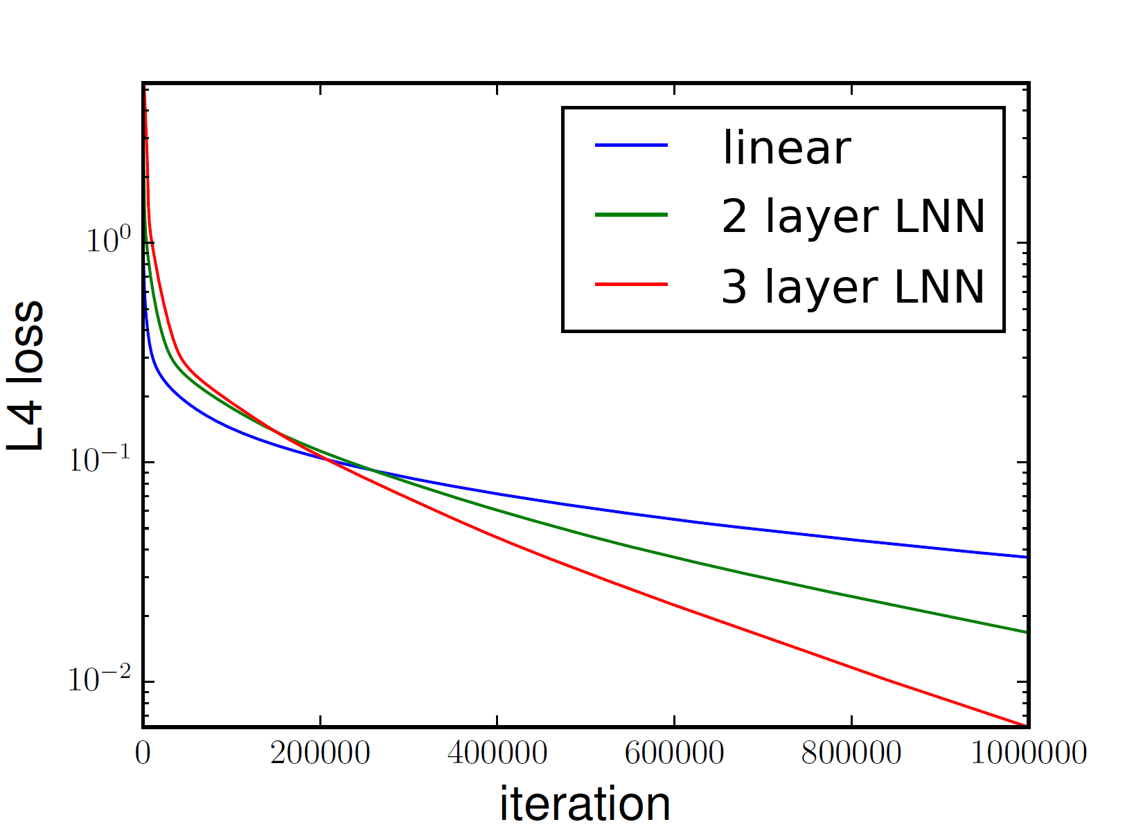
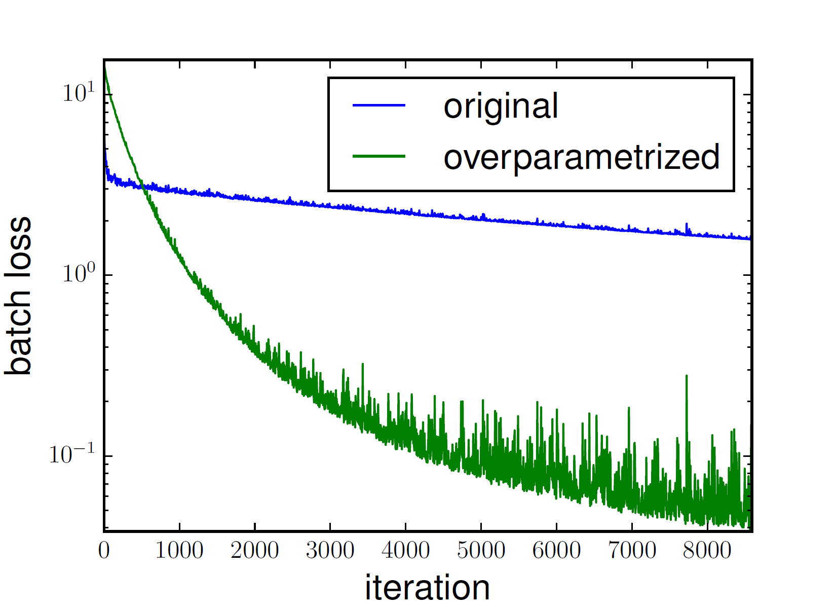
Figure 1: Empirical demonstrations of implicit acceleration by overparameterization, i.e. by replacement of linear transformations with linear neural networks. Left plot compares gradient descent applied to $\ell_{4}$ loss for a linear regression task (“linear”), against its application to the overparameterized objectives induced by two and three layer linear neural networks (“2 layer LNN” and “3 layer LNN,” respectively). Right plot compares stochastic gradient descent (with momentum) optimizing a non-linear convolutional neural network (“original”), against it optimizing a model obtained from replacing each dense linear transformation with a two layer linear neural network (“overparameterized”). For details see Arora et al. (2018), from which results are taken.

Subsection 3.1 employed the dynamical analysis of Section 2 to circumvent the difficulty in establishing convergence to global minimum using landscape arguments (see Proposition 3 and preceding text). In this subsection we discuss a result that further attests to the potential of dynamical analyses.

Classical machine learning is rooted in a preference for optimization to be convex. In our context, this means that if the loss $\ell(\cdot)$ is convex (setting of interest), optimizing it directly is preferred to doing so with a linear neural network, i.e. to minimizing the overparameterized objective $\phi(\cdot)$ defined in Equation (1) (this is because, as Proposition 1 in Section 2 shows, aside from degenerate cases, $\phi(\cdot)$ is non-convex). A surprising implication of the dynamical analysis from Section 2 is that such preference may be misleading — there exist cases where $\ell(\cdot)$ is convex, and yet its optimization via gradient descent is much slower than that of $\phi(\cdot)$. We present this result informally below, referring to Arora et al. (2018) for further details.

Claim 1 (informally stated).

Let $\epsilon>0$. Consider minimization of $\ell(\cdot)$ via gradient descent with (fixed) step size $\eta>0$, and denote by $t_{\ell,\eta}$ the index of the first iteration in which the value of $\ell(\cdot)$ is within $\epsilon$ from its global minimum (where $t_{\ell,\eta}:=\infty$ if this never takes place). Consider also a discrete minimization of $\phi(\cdot)$, or more precisely, a discretization with step size $\zeta>0$ of the end-to-end dynamics from Section 2 (with the notations of Corollary 1, this amounts to $vec\big{(}W^{(t+1)}\big{)}\mathrel{\reflectbox{$\mapsto$}}vec\big{(}W^{(t)}\big{)}-\zeta{\mathcal{P}}\big{(}W^{(t)}\big{)}vec\big{(}\nabla\ell(W^{(t)})\big{)}$ for $t\in{\mathbb{N}}\cup\{0\}$). Denote by $t_{\phi,\zeta}$ the index of the first iteration in this minimization where $\ell(\cdot)$ is within $\epsilon$ from its global minimum (if this never takes place then $t_{\phi,\zeta}:=\infty$). Denote by $t_{\ell}$ and $t_{\phi}$ the optimal convergence times over $\ell(\cdot)$ and $\phi(\cdot)$ respectively, i.e. $t_{\ell}:=\min_{\eta>0}t_{\ell,\eta}$ and $t_{\phi}:=\min_{\zeta>0}t_{\phi,\zeta}$. Let $c\in{\mathbb{R}}_{>0}$ be arbitrarily large, and let $p\in\{4,6,8,\ldots\}$. Then, there exist cases where $\ell(\cdot)$ is the $\ell_{p}$ loss for a linear regression task (i.e. it has the form $\ell(W)=\tfrac{1}{m}\sum\nolimits_{i=1}^{m}\|W{\mathbf{x}}_{i}-{\mathbf{y}}_{i}\|_{p}^{p}$ where ${\mathbf{x}}_{1},{\mathbf{x}}_{2},\ldots,{\mathbf{x}}_{m}\in{\mathbb{R}}^{d_{0}}$ are training instances and ${\mathbf{y}}_{1},{\mathbf{y}}_{2},\ldots,{\mathbf{y}}_{m}\in{\mathbb{R}}^{d_{n}}$ their corresponding labels), thus in particular is convex, and yet a near-zero initialization leads to $t_{\ell}>ct_{\phi}$.

Proof sketch.

Let $W^{*}$ be a global minimizer of $\ell(\cdot)$, and restrict attention to cases where it is unique. Since $\ell(\cdot)$ is the $\ell_{p}$ loss (for a linear regression task) with $p>2$, its landscape is steep away from $W^{*}$, and flat in the vicinity of $W^{*}$. This means (disregarding degenerate cases where $W^{*}$ is close to the origin) that with near-zero initialization, in order to reach $W^{*}$, optimization must initially descend a steep slope, and then traverse through a flat valley. If optimization is via gradient descent, a small step size is necessary to avoid divergence at the outset, and this leads to slow movement after the landscape flattens. On the other hand, the (discretized) end-to-end dynamics entail a preconditioner inducing a momentum effect (see text following Corollary 1), thus when applied with proper step size they can carefully descend to the flat valley, gradually accelerating thereafter. Depending on the location of $W^{*}$, this can result in arbitrarily faster convergence. ∎

The takeaway from Claim 1 is that overparameterization with a linear neural network, i.e. insertion of depth via linear layers, can accelerate gradient descent, despite introducing non-convexity while yielding no gain in terms of expressiveness! This phenomenon of implicit acceleration by overparameterization goes beyond the specific cases theoretically demonstrated in Claim 1. Namely, it occurs empirically in various cases where $\ell(\cdot)$ is the $\ell_{p}$ loss for a linear regression task with $p>2$ — see Figure 1 (left) for an example. Moreover, the phenomenon brings forth a practical technique for accelerating optimization of non-linear neural networks through addition of linear layers, i.e. through replacement of internal linear transformations with linear neural networks. This technique, demonstrated in Figure 1 (right), was employed in various real-world settings (see, e.g., Bell-Kligler et al. (2019); Guo et al. (2020); Cao et al. (2020); Huh et al. (2021)), and constitutes a practical application of linear neural networks born from a dynamical analysis.

4 Generalization

Neural networks are able to generalize even when having much more trainable parameters (weights) than examples to train on. The fact that this generalization can take place in the absence of any explicit regularization (see Zhang et al. (2017) for extensive empirical evidence) has led to a common view by which gradient-based optimization induces an implicit regularization — a tendency to fit training examples with functions of low “complexity.” It is an ongoing effort to mathematically support this intuition. The current section does so for linear neural networks.

Optimization of a linear neural network, i.e. minimization of the overparameterized objective $\phi(\cdot)$ (defined in Equation (1)), ultimately produces an end-to-end matrix $W_{n:1}$ (Definition 2) designed to be a solution for the loss $\ell(\cdot)$. The question we ask in this section is what kind of solution $W_{n:1}$ will be produced when $\phi(\cdot)$ is minimized via gradient descent emanating from near-zero initialization. This question is most meaningful when $\ell(\cdot)$ is underdetermined, i.e. admits multiple global minimizers. A prominent set of tasks giving rise to underdetermined loss functions is matrix sensing, which includes linear regression as a special case. We will focus on settings where $\ell(\cdot)$ corresponds to a matrix sensing task. Our treatment will rely on the dynamical analysis of Section 2.

4.1 Matrix Sensing

A matrix sensing task is defined by measurement matrices $A_{1},A_{2},\ldots$ $,A_{m}\in{\mathbb{R}}^{d_{n}\times d_{0}}$ and corresponding measurements $b_{1},b_{2},\ldots,b_{m}\in{\mathbb{R}}$. Given these, the goal is to find a matrix $W\in{\mathbb{R}}^{d_{n}\times d_{0}}$ satisfying ${\left\langle{W},{A_{i}}\right\rangle}:=\operatorname*{Tr}(WA_{i}^{\top})=b_{i}$ for $i=1,2,\ldots,m$. A notable special case of matrix sensing, known as matrix completion, is where each measurement matrix holds one in a single entry and zeros elsewhere. Linear regression is also a special case of matrix sensing, as for any ${\mathbf{x}}\in{\mathbb{R}}^{d_{0}}$ and ${\mathbf{y}}\in{\mathbb{R}}^{d_{n}}$, the requirement $W{\mathbf{x}}={\mathbf{y}}$ can be realized via $d_{n}$ measurement matrices ${\mathbf{e}}_{1}{\mathbf{x}}^{\top},{\mathbf{e}}_{2}{\mathbf{x}}^{\top},\ldots,{\mathbf{e}}_{d_{n}}{\mathbf{x}}^{\top}$ with corresponding measurements $y_{1},y_{2},\ldots,y_{d_{n}}$, where, for $i=1,2,\ldots,d_{n}$: ${\mathbf{e}}_{i}\in{\mathbb{R}}^{d_{n}}$ stands for a vector holding one in its $i$’th entry and zeros elsewhere; and $y_{i}\in{\mathbb{R}}$ represents the $i$’th entry of ${\mathbf{y}}$.

For tackling matrix sensing, it is common practice to consider the square loss over measurements. In our context this amounts to considering a training loss $\ell(\cdot)$ of the form:

$$\ell(W)=\tfrac{1}{2m}\sum\nolimits_{i=1}^{m}({\left\langle{W},{A_{i}}\right\rangle}-b_{i})^{2}\text{\,.}$$ (9)

If the number of measurements is smaller than the number of entries in the sought-after solution, i.e. $m<d_{0}d_{n}$, then (assuming the measurement matrices are linearly independent, which is generically the case) the loss $\ell(\cdot)$ is underdetermined — it admits infinitely many solutions attaining the global minimum $\ell^{*}:=\inf_{W\in{\mathbb{R}}^{d_{n}\times d_{0}}}\ell(W)=0$. There is often interest in finding, among all these global minimizers, one whose rank is lowest, i.e. $W^{*}\in\operatorname*{argmin}_{W\in{\mathbb{R}}^{d_{n}\times d_{0}}:\ell(W)=\ell^{*}}\operatorname*{Rank}(W)$. This is NP-hard in general. However, it is known (see Recht et al. (2010)) that if $\operatorname*{Rank}(W^{*})$ is sufficiently low compared to the number of measurements $m$, and if the measurement matrices satisfy a certain technical condition (“restricted isometry property”), then it is possible to find $W^{*}$ by solving a convex (constrained) optimization program, namely:

$$W^{*}=\operatorname*{argmin}\nolimits_{W\in{\mathbb{R}}^{d_{n}\times d_{0}}:\ell(W)=\ell^{*}}\|W\|_{*}\text{\,,}$$ (10)

where $\|\cdot\|_{*}$ stands for nuclear norm. Roughly speaking, this implies that in matrix sensing, given sufficiently many measurements, a global minimizer of lowest rank can often be found via regularization based on nuclear norm.

4.2 Implicit Regularization

Suppose we tackle matrix sensing with a linear neural network, meaning we optimize the overparameterized objective $\phi(\cdot)$ (Equation (1)) induced by a loss $\ell(\cdot)$ as defined in Equation (9). What kind of solution (for $\ell(\cdot)$) will the end-to-end matrix $W_{n:1}$ (Definition 2) reach? If any of the hidden dimensions of the network (i.e. any of $d_{1},d_{2},\ldots,d_{n-1}$) were small then $W_{n:1}$ would be constrained to have low rank, but as stated in Section 1, we consider the case where hidden dimensions are large enough to not restrict the search space (i.e. we assume $d_{j}\geq\min\{d_{0},d_{n}\}$ for $j=1,2,\ldots,n-1$). Surprisingly, experiments show (see, e.g., Arora et al. (2019b)) that even in this case, gradient descent with small step size emanating from near-zero initialization tends to produce an end-to-end matrix of low rank. This tendency is driven by implicit regularization, as there is nothing explicit in the optimized objective $\phi(\cdot)$ promoting low rank (indeed, it typically admits global minimizers whose end-to-end matrices have high rank).

Our goal in the current section is to mathematically characterize the implicit regularization described above, i.e. the tendency of linear neural networks to produce a low rank solution (end-to-end matrix) $W_{n:1}$ when applied to a loss $\ell(\cdot)$ of the form in Equation (9). An elegant supposition, formally stated below, is that the implicit regularization solves the convex optimization program in Equation (10), thus implements a method that under certain conditions provably finds a global minimizer of lowest rank.

Supposition 1.

If $W_{n:1}$ converges to a global minimizer (of $\ell(\cdot)$), this global minimizer has lowest nuclear norm (among all global minimizers).

Supposition 1 can be proven in scenarios where the measurement matrices $A_{1},A_{2},\ldots,A_{m}$ satisfy specific conditions (see Gunasekar et al. (2017); Li et al. (2018); Arora et al. (2019b); Belabbas (2020)). However, systematic experimentation suggests that it does not hold true in general — see Figure 2 for an example. In the next subsection we will employ the dynamical analysis of Section 2 for showing that the implicit regularization of linear neural networks implements a greedy low rank learning process which cannot be characterized as lowering nuclear norm, or any other norm.

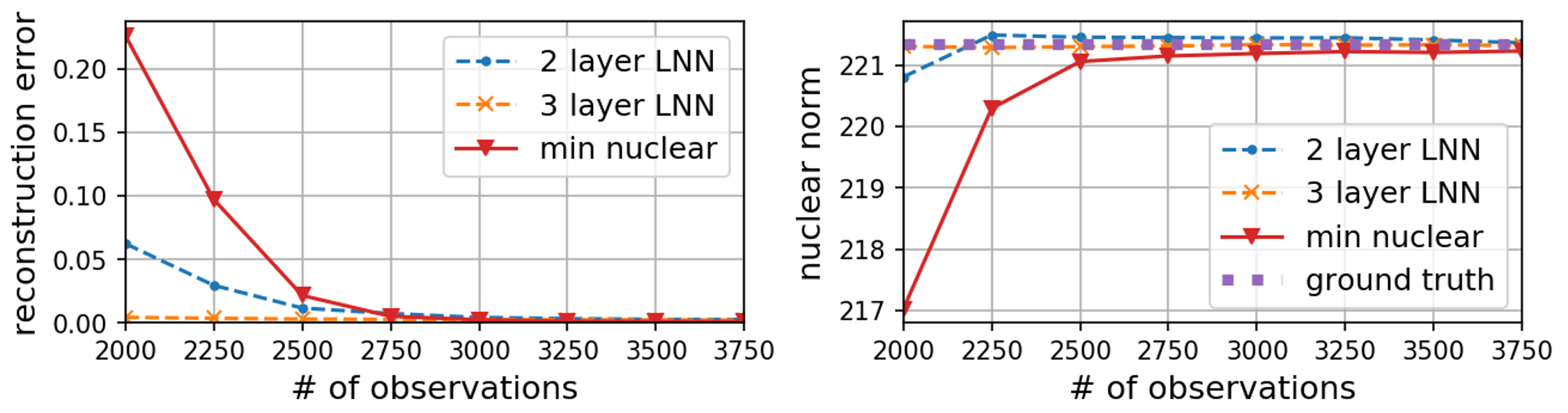
Figure 2: Experiment comparing, on matrix completion (special case of matrix sensing) tasks, the global minimizer of lowest nuclear norm (“min nuclear”) against solutions produced by two and three layer linear neural networks (“2 layer LNN” and “3 layer LNN,” respectively). Each task entails a different number of observations (measurements), taken from a low rank ground truth matrix. Left and right plots display reconstruction errors (distances from ground truth) and nuclear norms, respectively, of the solutions on each task. Notice that on tasks with many observations, the difference between ground truth and global minimizer of lowest nuclear norm is slight, and the linear neural networks converge to these. In contrast, on tasks with few observations the difference is significant, and the linear neural networks (especially the deeper one) choose low rank ground truth over global minimizer of lowest nuclear norm. For details see Arora et al. (2019b), from which results are taken.

4.3 Greedy Low Rank Learning

Our analysis of implicit regularization in linear neural networks relies on the concept of analytic singular value decomposition, defined herein for completeness.

Definition 4.

For a curve $W:[0,t_{e})\to{\mathbb{R}}^{d\times d^{\prime}}$, with $d,d^{\prime}\in{\mathbb{N}}$ and $t_{e}\in{\mathbb{R}}_{>0}\cup\{\infty\}$, an analytic singular value decomposition is a triplet $(U:[0,t_{e})\to{\mathbb{R}}^{d\times\underline{d}},S:[0,t_{e})\to{\mathbb{R}}^{\underline{d}\times\underline{d}},V:[0,t_{e})\to{\mathbb{R}}^{d^{\prime}\times\underline{d}})$, where $\underline{d}:=\min\{d,d^{\prime}\}$, the curves $U(\cdot)$, $S(\cdot)$ and $V(\cdot)$ are analytic,2 and for every $t\in[0,t_{e})$: the columns of $U(t)$ are orthonormal; $S(t)$ is diagonal; the columns of $V(t)$ are orthonormal; and $W(t)=U(t)S(t)V^{\top}(t)$.

Proposition 4 below states that the curve traversed by the end-to-end matrix (Definition 2) during optimization, i.e. $W_{n:1}(\cdot)$, admits an analytic singular value decomposition.

Proposition 4.

There exists an analytic singular value decomposition for $W_{n:1}(\cdot)$.

Proof.

Any analytic curve in matrix space admits an analytic singular value decomposition (see Theorem 1 in Bunse-Gerstner et al. (1991)), so it suffices to show that $W_{n:1}(\cdot)$ is analytic. Analytic functions are closed under summation, multiplication and composition, so the analyticity of the loss $\ell(\cdot)$ implies that the overparameterized objective $\phi(\cdot)$ (Equation (1)) is analytic as well. A basic result in the theory of analytic differential equations is that gradient flow over an analytic objective yields an analytic curve (see Theorem 1.1 in Ilyashenko and Yakovenko (2008)). We conclude that $W_{1}(\cdot),W_{2}(\cdot),\ldots,W_{n}(\cdot)$ (curves traversed by the weight matrices during optimization; see Equation (2)) are analytic. Since $W_{n:1}(\cdot):=W_{n}(\cdot)W_{n-1}(\cdot)\cdots W_{1}(\cdot)$, and, as stated, analytic functions are closed under summation and multiplication, $W_{n:1}(\cdot)$ is also analytic. This concludes the proof. ∎

Let $(U(\cdot),S(\cdot),V(\cdot))$ be an analytic singular value decomposition for $W_{n:1}(\cdot)$. For $r=1,2,\ldots,\min\{d_{0},d_{n}\}$, denote by ${\mathbf{u}}_{r}(\cdot)$ the $r$’th column of $U(\cdot)$, by $\sigma_{r}(\cdot)$ the $r$’th diagonal entry of $S(\cdot)$, and by ${\mathbf{v}}_{r}(\cdot)$ the $r$’th column of $V(\cdot)$. Up to potential minus signs, $(\sigma_{r}(\cdot))_{r=1}^{\min\{d_{0},d_{n}\}}$ are the singular values of $W_{n:1}(\cdot)$, with corresponding left and right singular vectors $({\mathbf{u}}_{r}(\cdot))_{r=1}^{\min\{d_{0},d_{n}\}}$ and $({\mathbf{v}}_{r}(\cdot))_{r=1}^{\min\{d_{0},d_{n}\}}$, respectively. The following theorem employs the end-to-end dynamics from Section 2 (Theorem 1) for characterizing the dynamics of $\sigma_{r}(\cdot)$.

Theorem 3.

It holds that:

$$\dot{\sigma}_{r}(t):=\tfrac{d}{dt}\sigma_{r}(t)=\big{(}\sigma_{r}^{2}(t)\big{)}^{1-1/n}{\left\langle{-\nabla\ell\big{(}W_{n:1}(t)\big{)}},{{\mathbf{u}}_{r}(t){\mathbf{v}}_{r}^{\top}(t)}\right\rangle}n~{},~{}~{}t>0~{},~{}r=1,2,\ldots,\min\{d_{0},d_{n}\}\text{\,,}$$

where as before, ${\left\langle{\cdot\,},{\cdot}\right\rangle}$ stands for the standard inner product between matrices, i.e. ${\left\langle{A},{B}\right\rangle}:=\operatorname*{Tr}(AB^{\top})$ for any matrices $A$ and $B$ of the same dimensions.

Proof.

Differentiating the analytic singular value decomposition of $W_{n:1}(\cdot)$ with respect to time yields:

$$\dot{W}_{n:1}(t)=\dot{U}(t)S(t)V^{\top}(t)+U(t)\dot{S}(t)V^{\top}(t)+U(t)S(t)\dot{V}^{\top}(t)~{},~{}~{}t>0\text{\,,}$$

where $\dot{U}(t):=\tfrac{d}{dt}U(t)$, $\dot{S}(t):=\tfrac{d}{dt}S(t)$ and $\dot{V}(t):=\tfrac{d}{dt}V(t)$. Multiplying from the left by $U^{\top}(t)$ and from the right by $V(t)$, while using the fact that the columns of $U(t)$ are orthonormal and the columns of $V(t)$ are orthonormal, we obtain:

$$U^{\top}(t)\dot{W}_{n:1}(t)V(t)=U^{\top}(t)\dot{U}(t)S(t)+\dot{S}(t)+S(t)\dot{V}^{\top}(t)V(t)~{},~{}~{}t>0\text{\,.}$$

Fix some $r\in\{1,2,\ldots,\min\{d_{0},d_{n}\}\}$. The $r$’th diagonal entry of the latter matrix equation is:

$${\mathbf{u}}_{r}^{\top}(t)\dot{W}_{n:1}(t){\mathbf{v}}_{r}(t)={\mathbf{u}}_{r}^{\top}(t)\dot{{\mathbf{u}}}_{r}(t)\cdot\sigma_{r}(t)+\dot{\sigma}_{r}(t)+\sigma_{r}(t)\cdot\dot{{\mathbf{v}}}_{r}^{\top}(t){\mathbf{v}}_{r}(t)~{},~{}~{}t>0\text{\,,}$$ (11)

where $\dot{{\mathbf{u}}}_{r}(t):=\tfrac{d}{dt}{\mathbf{u}}_{r}(t)$ and $\dot{{\mathbf{v}}}_{r}(t):=\tfrac{d}{dt}{\mathbf{v}}_{r}(t)$. Since ${\mathbf{u}}_{r}(\cdot)$ is a column of $U(\cdot)$ it has unit length throughout, meaning ${\mathbf{u}}_{r}^{\top}(\cdot){\mathbf{u}}_{r}(\cdot)\equiv 1$. Similarly, ${\mathbf{v}}_{r}(\cdot)$ is a column of $V(\cdot)$ and therefore ${\mathbf{v}}_{r}^{\top}(\cdot){\mathbf{v}}_{r}(\cdot)\equiv 1$. This implies that for every $t>0$:

$${\mathbf{u}}_{r}^{\top}(t)\dot{{\mathbf{u}}}_{r}(t)=\tfrac{1}{2}\tfrac{d}{dt}\big{(}{\mathbf{u}}_{r}^{\top}(t){\mathbf{u}}_{r}(t)\big{)}=0\text{~{}~{}~{}and~{}~{}~{}}\dot{{\mathbf{v}}}_{r}^{\top}(t){\mathbf{v}}_{r}(t)=\tfrac{1}{2}\tfrac{d}{dt}\big{(}{\mathbf{v}}_{r}^{\top}(t){\mathbf{v}}_{r}(t)\big{)}=0\text{\,.}$$

Equation (11) thus simplifies to:

$$\dot{\sigma}_{r}(t)={\mathbf{u}}_{r}^{\top}(t)\dot{W}_{n:1}(t){\mathbf{v}}_{r}(t)~{},~{}~{}t>0\text{\,.}$$

Plugging in the end-to-end dynamics (Equation (3)), we have:

$$\dot{\sigma}_{r}(t)=-\sum\nolimits_{j=1}^{n}{\mathbf{u}}_{r}^{\top}(t)\left[W_{n:1}(t)W_{n:1}^{\top}(t)\right]^{\frac{j-1}{n}}\nabla\ell\big{(}W_{n:1}(t)\big{)}\left[W_{n:1}^{\top}(t)W_{n:1}(t)\right]^{\frac{n-j}{n}}{\mathbf{v}}_{r}(t)~{},~{}~{}t>0\text{\,.}$$ (12)

For every $t>0$ and $j\in\{1,2,\ldots,n\}$:

$${\mathbf{u}}_{r}^{\top}(t)\left[W_{n:1}(t)W_{n:1}^{\top}(t)\right]^{\frac{j-1}{n}}={\mathbf{u}}_{r}^{\top}(t)U(t)\left[S^{2}(t)\right]^{\frac{j-1}{n}}U^{\top}(t)=\big{(}\sigma_{r}^{2}(t)\big{)}^{\frac{j-1}{n}}\cdot{\mathbf{u}}_{r}^{\top}(t)$$ (13)

and

$$\left[W_{n:1}^{\top}(t)W_{n:1}(t)\right]^{\frac{n-j}{n}}{\mathbf{v}}_{r}(t)=V(t)\left[S^{2}(t)\right]^{\frac{n-j}{n}}V^{\top}(t){\mathbf{v}}_{r}(t)=\big{(}\sigma_{r}^{2}(t)\big{)}^{\frac{n-j}{n}}\cdot{\mathbf{v}}_{r}(t)\text{\,.}$$ (14)

Plugging Equations (13) and (14) into Equation (12) concludes the proof:

$$\begin{split}\dot{\sigma}_{r}(t)&=-\sum\nolimits_{j=1}^{n}\big{(}\sigma_{r}^{2}(t)\big{)}^{1-1/n}\cdot{\mathbf{u}}_{r}^{\top}(t)\nabla\ell\big{(}W_{n:1}(t)\big{)}{\mathbf{v}}_{r}(t)\\ &=\big{(}\sigma_{r}^{2}(t)\big{)}^{1-1/n}{\left\langle{-\nabla\ell\big{(}W_{n:1}(t)\big{)}},{{\mathbf{u}}_{r}(t){\mathbf{v}}_{r}^{\top}(t)}\right\rangle}n\end{split}~{}~{},~{}~{}t>0\text{\,.}$$

∎

An immediate implication of Theorem 3 is that in the case where $W_{n:1}(\cdot)$ is square (i.e. where $d_{0}=d_{n}$), its determinant does not change sign.

Lemma 2.

Assume that $d_{0}=d_{n}$. Then, the sign of $\mathrm{det}\big{(}W_{n:1}(\cdot)\big{)}$ is constant through time. That is, one of the following holds: (i) $\mathrm{det}\big{(}W_{n:1}(t)\big{)}\,{>}\,0$ for all $t\,{\geq}\,0$; (ii) $\mathrm{det}\big{(}W_{n:1}(t)\big{)}\,{=}\,0$ for all $t\,{\geq}\,0$; or (iii) $\mathrm{det}\big{(}W_{n:1}(t)\big{)}\,{<}\,0$ for all $t\,{\geq}\,0$.

Proof.

Since $\abs{\mathrm{det}\big{(}W_{n:1}(\cdot)\big{)}}\,{=}\,\prod_{r=1}^{d_{0}}\abs{\sigma_{r}(\cdot)}$, by the continuity of $\mathrm{det}\big{(}W_{n:1}(\cdot)\big{)},(\sigma_{r}(\cdot))_{r=1}^{d_{0}}$ and the intermediate value theorem, it suffice to show that for each $r\in\{1,2,\ldots,d_{0}\}$ either $\sigma_{r}(t)\neq 0$ for all $t\geq 0$ or $\sigma_{r}(t)=0$ for all $t\geq 0$.

Fix some $r\in\{1,2,\ldots,d_{0}\}$, and let $g(\cdot)$ be the function defined by:

$$g(t):=\left\langle{-\nabla\ell\big{(}W_{n:1}(t)\big{)}},{{\mathbf{u}}_{r}(t){\mathbf{v}}_{r}^{\top}(t)}\right\rangle n~{},~{}~{}t\geq 0\text{\,.}$$

By Theorem 3 it holds that $\dot{\sigma}_{r}(t)=\big{(}\sigma_{r}^{2}(t)\big{)}^{1-1/n}g(t)$ for all $t>0$. It can be verified via differentiation that the solution of this differential equation is, when $n=2$:

$$\sigma_{r}(t)=\begin{cases}\sigma_{r}(0)\exp\big{(}\int\nolimits_{0}^{t}g(t^{\prime})\,dt^{\prime}\big{)}&\text{if}~{}\sigma_{r}(0)>0\text{\,,}\\[1.42262pt] \sigma_{r}(0)\exp\big{(}-\int\nolimits_{0}^{t}g(t^{\prime})\,dt^{\prime}\big{)}&\text{if}~{}\sigma_{r}(0)<0\text{\,,}\\[1.42262pt] 0&\text{otherwise\,,}\end{cases}\qquad t\geq 0\text{\,,}$$

and when $n\geq 3$:

$$\sigma_{r}(t)=\begin{cases}\Big{(}\big{(}\sigma_{r}(0)\big{)}^{2/n-1}+(2/n-1)\int\nolimits_{0}^{t}g(t^{\prime})dt^{\prime}\Big{)}^{\frac{1}{2/n-1}}&\text{if}~{}\sigma_{r}(0)>0\text{\,,}\\ -\Big{(}\big{(}-\sigma_{r}(0)\big{)}^{2/n-1}-(2/n-1)\int\nolimits_{0}^{t}g(t^{\prime})dt^{\prime}\Big{)}^{\frac{1}{2/n-1}}&\text{if}~{}\sigma_{r}(0)<0\text{\,,}\\[5.69054pt] 0&\text{otherwise\,,}\end{cases}\qquad t\geq 0\text{\,.}$$

Whether $n=2$ or $n\geq 3$, it holds that either $\sigma_{r}(t)\neq 0$ for all $t\geq 0$ or $\sigma_{r}(t)=0$ for all $t\geq 0$. This concludes the proof. ∎

Lemma 2 has a far reaching consequence: there exist cases where $\ell(\cdot)$ corresponds to a matrix sensing task (i.e. is of the form in Equation (9)), and its minimization leads all norms of $W_{n:1}(\cdot)$ to grow towards infinity. This result — formally delivered by Proposition 5 below — contrasts Supposition 1 in that it means the implicit regularization of linear neural networks in matrix sensing cannot be characterized as lowering any norm, in particular the nuclear norm.

Proposition 5.

Assume that $d_{0}=d_{n}$. Then, there exist measurement matrices $A_{1},A_{2},\ldots,A_{m}\in{\mathbb{R}}^{d_{n}\times d_{0}}$ and corresponding measurements $b_{1},b_{2},\ldots,b_{m}\in{\mathbb{R}}$ such that the loss $\ell(\cdot)$ defined by Equation (9) admits (finite) solutions attaining the global minimum $\ell^{*}:=\inf_{W\in{\mathbb{R}}^{d_{n}\times d_{0}}}\ell(W)=0$, and yet the following holds. For any norm $\|\cdot\|$ over ${\mathbb{R}}^{d_{n}\times d_{0}}$, there exist constants $c\in{\mathbb{R}}_{>0}$ and $c^{\prime}\in{\mathbb{R}}$ such that if $\mathrm{det}\big{(}W_{n:1}(0)\big{)}>0$, i.e. if the determinant of the end-to-end matrix is positive at initialization, then:

$$\|W_{n:1}(t)\|\geq c\big{(}\ell\big{(}W_{n:1}(t)\big{)}-\ell^{*}\big{)}^{-1/2}+c^{\prime}~{},~{}t\geq 0\text{\,,}$$

meaning in particular that $\|W_{n:1}(\cdot)\|$ diverges to infinity when the loss approaches global minimum (i.e. when $\ell\big{(}W_{n:1}(\cdot)\big{)}$ converges to $\ell^{*}$).

Proof.

For simplicity of presentation, suppose that $d_{0}=d_{n}=2$. Appendix B in Razin and Cohen (2020) outlines an extension to arbitrary dimensions. Consider the measurement matrices $A_{1}={\mathbf{e}}_{1}{\mathbf{e}}_{2}^{\top},A_{2}={\mathbf{e}}_{2}{\mathbf{e}}_{1}^{\top},A_{3}={\mathbf{e}}_{2}{\mathbf{e}}_{2}^{\top}\in{\mathbb{R}}^{2\times 2}$, where ${\mathbf{e}}_{1}$ and ${\mathbf{e}}_{2}$ are the standard basis vectors of ${\mathbb{R}}^{2}$, and corresponding measurements $b_{1}=b_{2}=1$ and $b_{3}=0$. The loss (Equation (9)) in this case can be written as:

$$\ell(W)=\frac{1}{6}\left[(w_{1,2}-1)^{2}+(w_{2,1}-1)^{2}+w_{2,2}^{2}\right]\text{\,,}$$

where $w_{i,j}$ denotes the $(i,j)$’th entry of $W\in{\mathbb{R}}^{2\times 2}$, for $i=1,2$ and $j=1,2$. Clearly, any $W\in{\mathbb{R}}^{2\times 2}$ holding ones on its off-diagonal and zero at its bottom right entry attains zero loss, i.e. $\ell(W)=\ell^{*}=0$.

Now, fix some time $t\geq 0$ and assume that $\ell(W_{n:1}(t))<\frac{1}{6}$. Later this assumption will be lifted. Denoting by $w_{i,j}(t)$ the $(i,j)$’th entry of $W_{n:1}(t)$, for $i=1,2$ and $j=1,2$, we can straightforwardly bound $w_{1,2}(t),w_{2,1}(t)$ and $w_{2,2}(t)$ as a function of $\ell(W_{n:1}(t))$ as follows:

$$\abs{w_{1,2}(t)-1}\leq\sqrt{6\ell(W_{n:1}(t))}~{}~{}~{},~{}~{}~{}\abs{w_{2,1}(t)-1}\leq\sqrt{6\ell(W_{n:1}(t))}~{}~{}~{},~{}~{}~{}\abs{w_{2,2}(t)}\leq\sqrt{6\ell(W_{n:1}(t))}\text{\,.}$$ (15)

By Lemma 2 the determinant of $W_{n:1}(\cdot)$ does not change sign during optimization. Since $\mathrm{det}(W_{n:1}(0))>0$, this implies that:

$$\mathrm{det}\big{(}W_{n:1}(t)\big{)}=w_{1,1}(t)\cdot w_{2,2}(t)-w_{1,2}(t)\cdot w_{2,1}(t)>0\text{\,.}$$ (16)

Equation 15, along with our assumption that $\ell(W_{n:1}(t))<\frac{1}{6}$, ensures that $w_{1,2}(t),w_{2,1}(t)>0$. Thus, for $\mathrm{det}\big{(}W_{n:1}(t)\big{)}$ to be positive, necessarily $w_{1,1}(t)\cdot w_{2,2}(t)>0$. Rearranging Equation (16), we may therefore write $\abs{w_{1,1}(t)\cdot w_{2,2}(t)}=w_{1,1}(t)\cdot w_{2,2}(t)>w_{1,2}(t)\cdot w_{2,1}(t)$. Then, dividing by $\abs{w_{2,2}(t)}$ and applying the bounds from Equation (15) leads to:

$$\abs{w_{1,1}(t)}>\frac{\brk 1{1-\sqrt{6\ell(W_{n:1}(t))}}^{2}}{\sqrt{6\ell(W_{n:1}(t))}}=\frac{1}{\sqrt{6\ell(W_{n:1}(t))}}-2+\sqrt{6\ell(W_{n:1}(t))}\geq\frac{1}{\sqrt{6\ell(W_{n:1}(t))}}-2\text{\,.}$$

It remains to convert this lower bound on $\abs{w_{1,1}(t)}$ into a lower bound on $\norm{W_{n:1}(t)}$. This is done via the triangle inequality:

$$\norm{W_{n:1}(t)}\geq\abs{w_{1,1}(t)}\cdot\norm{{\mathbf{e}}_{1}{\mathbf{e}}_{1}^{\top}}-\norm{W_{n:1}(t)-w_{1,1}(t)\cdot{\mathbf{e}}_{1}{\mathbf{e}}_{1}^{\top}}\text{\,.}$$

We can bound the negative term on the right hand side by Equation (15) and another application of the triangle inequality:

$$\begin{split}\norm{W_{n:1}(t)-w_{1,1}(t)\cdot{\mathbf{e}}_{1}{\mathbf{e}}_{1}^{\top}}&\leq\big{(}1+\sqrt{6\ell(W_{n:1}(t))}\big{)}\cdot\big{(}\norm{{\mathbf{e}}_{1}{\mathbf{e}}_{2}^{\top}}+\norm{{\mathbf{e}}_{2}{\mathbf{e}}_{1}^{\top}}\big{)}+\sqrt{6\ell(W_{n:1}(t))}\cdot\norm{{\mathbf{e}}_{2}{\mathbf{e}}_{2}^{\top}}\\ &\leq 2\big{(}\norm{{\mathbf{e}}_{1}{\mathbf{e}}_{2}^{\top}}+\norm{{\mathbf{e}}_{2}{\mathbf{e}}_{1}^{\top}}+\norm{{\mathbf{e}}_{2}{\mathbf{e}}_{2}^{\top}}\big{)}\text{\,,}\end{split}$$

where the last transition is by our assumption that $\ell(W_{n:1}(t))<\frac{1}{6}$. Then, from the lower bound on $\abs{w_{1,1}(t)}$ it follows that:

$$\norm{W_{n:1}(t)}\geq\frac{1}{\sqrt{6\ell(W_{n:1}(t))}}\cdot\norm{{\mathbf{e}}_{1}{\mathbf{e}}_{1}^{\top}}-2\big{(}\norm{{\mathbf{e}}_{1}{\mathbf{e}}_{1}^{\top}}+\norm{{\mathbf{e}}_{1}{\mathbf{e}}_{2}^{\top}}+\norm{{\mathbf{e}}_{2}{\mathbf{e}}_{1}^{\top}}+\norm{{\mathbf{e}}_{2}{\mathbf{e}}_{2}^{\top}}\big{)}\text{\,.}$$

Defining the constants $c:=\norm{{\mathbf{e}}_{1}{\mathbf{e}}_{1}^{\top}}/\sqrt{6}$ and $c^{\prime}:=\min\big{\{}-\sqrt{6}c,-2\big{(}\norm{{\mathbf{e}}_{1}{\mathbf{e}}_{1}^{\top}}+\norm{{\mathbf{e}}_{1}{\mathbf{e}}_{2}^{\top}}+\norm{{\mathbf{e}}_{2}{\mathbf{e}}_{1}^{\top}}+\norm{{\mathbf{e}}_{2}{\mathbf{e}}_{2}^{\top}}\big{)}\big{\}}$, while recalling that $\ell^{*}=0$, we arrive at:

$$\|W_{n:1}(t)\|\geq c\big{(}\ell\big{(}W_{n:1}(t)\big{)}-\ell^{*}\big{)}^{-1/2}+c^{\prime}\text{\,.}$$

Lastly, to lift our assumption that $\ell(W_{n:1}(t))<\frac{1}{6}$, notice that when $\ell(W_{n:1}(t))\geq\frac{1}{6}$ the lower bound trivially holds as it is non-positive. ∎

The inability of norms to explain the implicit regularization under study (i.e. that of linear neural networks in matrix sensing) poses a quandary, as from a classical machine learning perspective, regularization is typically norm-based. To overcome this quandary we return to Theorem 3, which provides an alternative explanation by revealing a form of greedy low rank learning. Namely, it reveals that each $\sigma_{r}(\cdot)$, i.e. each singular value of $W_{n:1}(\cdot)$, evolves at a rate given by a product of two factors: (i) ${\left\langle{-\nabla\ell\big{(}W_{n:1}(\cdot)\big{)}},{{\mathbf{u}}_{r}(\cdot){\mathbf{v}}_{r}^{\top}(\cdot)}\right\rangle}n$, which implies that $\sigma_{r}(\cdot)$ moves faster when its singular component (i.e. ${\mathbf{u}}_{r}(\cdot){\mathbf{v}}_{r}^{\top}(\cdot)$) is more aligned with the direction of steepest descent in the loss (i.e. with $-\nabla\ell(W_{n:1}(\cdot))$); and (ii) $(\sigma_{r}^{2}(\cdot))^{1-1/n}$, by which the speed of $\sigma_{r}(\cdot)$ is proportional to its size exponentiated by $2-2/n$. The second factor creates a momentum-like effect, which attenuates the movement of small singular values and accelerates the movement of large ones. Accordingly, we may expect that with near-zero initialization (regime of interest), singular values progress slowly at first, and then, one after the other they reach a critical threshold and quickly rise, until convergence is attained. Such dynamics can be viewed as a greedy learning process which incrementally increases the rank of its search space, thereby entailing a preference for solutions of low rank. This greedy low rank learning process indeed takes place empirically, and moreover, in accordance with the fact that the exponent $2-2/n$ grows with $n$ (number of layers in the linear neural network), the process sharpens with depth — see Figure 3 for an example. We note that under certain conditions, Theorem 3 can be used to derive closed-form expressions for $(\sigma_{r}(\cdot))_{r=1}^{\min\{d_{0},d_{n}\}}$ (see Arora et al. (2019b)), or to formally prove that the global minimizer to which $W_{n:1}(\cdot)$ converges has low rank (analogously to the results of Li et al. (2021); Razin et al. (2021); Jin et al. (2023)).

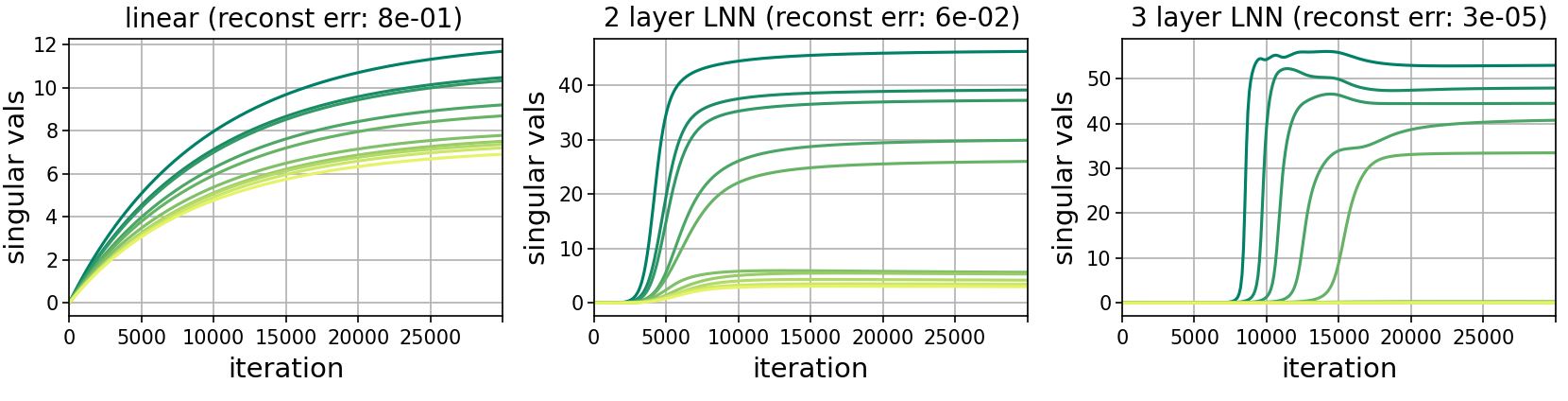
Figure 3: Empirical demonstration of the greedy low rank learning process implemented by the implicit regularization of linear neural networks. Plots show, for a matrix sensing task comprising measurements taken from a low rank ground truth, singular values of the learned solution throughout the iterations of gradient descent. Left (“linear”) plot corresponds to direct minimization of the matrix sensing loss; middle (“2 layer LNN”) and right (“3 layer LNN”) plots correspond to minimization of the overparameterized objectives induced by two and three layer linear neural networks, respectively. Plot titles specify reconstruction error (distance of learned solution from ground truth matrix) at the end of training. Notice that the greedy low rank learning process takes place only with the linear neural networks, and is sharper with the deeper network. For details see Arora et al. (2019b), from which results are taken.

4.4 Implicit Compression by Overparameterization

Recall from Subsection 3.2 that overparameterization, i.e. replacement of a linear transformation with a linear neural network, can accelerate optimization. The results of the current section imply that it also encourages convergence to solutions of low rank, meaning ones that can be compressed. This phenomenon — an implicit compression by overparameterization — facilitates a practical technique of adding linear layers for fitting training data with a reduced-size model, thereby improving both generalization and computational efficiency at inference time. The technique has been applied to non-linear neural networks in various real-world settings (see, e.g., Guo et al. (2020); Jing et al. (2020); Huh et al. (2021)). Similarly to acceleration of optimization by overparameterization (see Subsection 3.2), it constitutes a practical application of linear neural networks born from a dynamical analysis.

5 Extension: Arithmetic Neural Networks

Linear neural networks are a fundamental model in the theory of deep learning, and as discussed in Subsections 3.2 and 4.4, they also admit practical benefits. Nevertheless, they are limited to linear (input-output) mappings, thus fail to capture the crucial role of non-linearity in deep learning. In this section we briefly discuss a non-linear extension of linear neural networks that is closer to practical deep learning.

Linear neural networks can be viewed as matrix factorizations, in accordance with the fact that the mappings they realize are naturally represented as matrices factorized by network weights. Lifting matrices (two-dimensional arrays) to higher dimensions, i.e. considering tensor factorizations (or more precisely, mappings represented as tensors factorized by network weights), gives rise to neural networks with multiplicative non-linearity, known as arithmetic neural networks. Arithmetic neural networks have been shown to exhibit promising empirical performance (see, e.g., Cohen et al. (2016a); Sharir et al. (2016); Chrysos et al. (2021)), and their expressiveness was the subject of numerous theoretical studies (see, e.g., Cohen et al. (2016b); Cohen and Shashua (2016; 2017); Cohen et al. (2017; 2018); Sharir and Shashua (2018); Levine et al. (2018a; b); Balda et al. (2018); Khrulkov et al. (2018; 2019); Levine et al. (2019); Alexander et al. (2023); Razin et al. (2023)). It is possible to extend some of the (linear neural network) results in these lecture notes to arithmetic neural networks. In particular, through a dynamical analysis, it can be shown that — similarly to how the implicit regularization of linear neural networks lowers matrix rank — the implicit regularization of arithmetic neural networks lowers tensor ranks. For details see Razin et al. (2021) and Razin et al. (2022).

6 Conclusion

These lecture notes presented a theory of linear neural networks — a fundamental model in the study of optimization and generalization in deep learning. At the heart of the theory lies a dynamical characterization, by which training a linear neural network is equivalent to training a linear mapping with a certain preconditioner that promotes movement in directions already taken (Section 2). The dynamical characterization facilitated two results concerning optimization (Section 3): (i) a guarantee of convergence to global minimum, applicable to linear neural networks of arbitrary depth (Subsection 3.1); and (ii) a proof that there exist cases where insertion of depth via linear layers can accelerate training, despite introducing non-convexity while yielding no gain in terms of expressiveness (Subsection 3.2). With regards to generalization, the dynamical characterization was used to show that the implicit regularization of linear neural networks implements a greedy low rank learning process, which cannot be characterized as lowering any norm (Section 4). Practical applications born from the presented theory — namely, techniques for improving optimization, generalization and computational efficiency of non-linear neural networks — were discussed (Subsections 3.2 and 4.4).

The dynamical approach underlying the presented theory was shown to overcome limitations of other theoretical approaches. For example: (i) it established a convergence guarantee (Theorem 2) in the presence of non-strict saddle points (Proposition 3), i.e. in a setting where generic landscape arguments from the literature on non-convex optimization (see, e.g., Ge et al. (2015); Lee et al. (2016)) are invalid; (ii) it proved that non-convex training of a linear neural network can be much faster than convex training of a linear mapping (Claim 1), a conclusion that cannot be attained through the classical lens by which convex training is preferable; and (iii) it provided a description of implicit regularization (Theorem 3) applicable to settings where no norm is being lowered (Proposition 5), i.e. where the standard association between regularization and norms (cf. Supposition 1) is inappropriate. Dynamical approaches have recently been adopted beyond the context of linear neural networks, e.g. for analyzing arithmetic neural networks (see Section 5). We hypothesize that such approaches will be key to developing a complete theoretical understanding of deep learning.

Exercises

Exercise 1.

Consider the expression for the end-to-end dynamics given in Theorem 1 (Equation (3)). Simplify this expression for the case of a single output variable (i.e., $d_{n}=1$), and explain how the simplified form resonates with the interpretation of the end-to-end dynamics as promoting movement in directions already taken.

Exercise 2.

In this exercise you will derive a variant of the end-to-end dynamics (Theorem 1) that applies to a two layer symmetric linear neural network, i.e. to the parametric family of hypotheses $\{{\mathbf{x}}\mapsto WW^{\top}{\mathbf{x}}:W\in{\mathbb{R}}^{d\times d}\}$, where $d\in{\mathbb{N}}$. Let $\ell_{s}:{\mathbb{R}}^{d\times d}\to{\mathbb{R}}$ be an analytic training loss, and consider the induced objective:

$$\phi_{s}:{\mathbb{R}}^{d\times d}\to{\mathbb{R}}~{},~{}\phi_{s}(W)=\ell_{s}(WW^{\top})\text{\,.}$$

Suppose we run gradient flow over $\phi_{s}(\cdot)$, meaning we generate a continuous curve $W(\cdot)$ in ${\mathbb{R}}^{d\times d}$ via the following differential equation:

$$\dot{W}(t):=\tfrac{d}{dt}W(t)=-\nabla\phi_{s}(W(t))~{},~{}t>0\text{\,.}$$

Derive a self-contained expression for the dynamics of the curve $W_{s}(\cdot):=W(\cdot)W(\cdot)^{\top}$. Specifically, derive an expression for $\dot{W}_{s}(t):=\tfrac{d}{dt}W_{s}(t)$, where $t>0$, that depends on $W(t)$ only via $W_{s}(t)$ (meaning the expression may include $W_{s}(t)$ but not $W(t)$).

Exercise 3.

Prove the following result, used in Example 1. For any $d,d^{\prime}\in{\mathbb{N}}$, $W\in{\mathbb{R}}^{d\times d^{\prime}}$ and $\delta>0$, it holds that:

$$\min\big{\{}\|W-W^{\prime}\|_{F}:W^{\prime}\in{\mathbb{R}}^{d\times d^{\prime}},\sigma_{\min}(W^{\prime})\leq\delta\big{\}}=\max\big{\{}0,\sigma_{\min}(W)-\delta\big{\}}\text{\,,}$$

where $\|\cdot\|_{F}$ stands for Frobenius norm and $\sigma_{\min}(\cdot)$ refers to the minimal singular value of a matrix. You may use without proof the fact that $\|W-W^{\prime}\|_{F}\geq\|{\boldsymbol{\sigma}}(W)-{\boldsymbol{\sigma}}(W^{\prime})\|_{2}$, where ${\boldsymbol{\sigma}}(W)$ and ${\boldsymbol{\sigma}}(W^{\prime})$ are the vectors in ${\mathbb{R}}^{\min\{d,d^{\prime}\}}$ holding, in non-increasing order, the singular values of $W$ and $W^{\prime}$ respectively (see Exercise IV.3.5 in Bhatia (1997)).

Exercise 4.

Suppose we modify the statement of Proposition 5 by replacing the condition $\mathrm{det}\big{(}W_{n:1}(0)\big{)}>0$ with $\mathrm{det}\big{(}W_{n:1}(0)\big{)}<0$. Adapt the proof of the proposition such that it accords with the modified statement.

Exercise 5.

Consider the singular value dynamics from Theorem 3, in the special case where the linear neural network has two layers, i.e. $n=2$. Let $(c_{r})_{r=1}^{\min\{d_{0},d_{2}\}}$ be a tuple of distinct real numbers. Let $\epsilon>0$ and $t_{e}>0$. Assume that, for $r=1,2,\ldots,\min\{d_{0},d_{2}\}$:

• $\sigma_{r}(\cdot)$ equals $\epsilon$ at initialization (i.e. $\sigma_{r}(0)=\epsilon$); and

• $\langle-\nabla\ell(W_{2:1}(\cdot)),{\mathbf{u}}_{r}(\cdot){\mathbf{v}}_{r}^{\top}(\cdot)\rangle$ is fixed at $c_{r}$ until time $t_{e}$ of optimization (i.e. for all $t\in[0,t_{e}]$ it holds that $\langle-\nabla\ell(W_{n:1}(t)),{\mathbf{u}}_{r}(t){\mathbf{v}}_{r}^{\top}(t)\rangle=c_{r}$).

Derive closed-form expressions for $(\sigma_{r}(t))_{r=1}^{\min\{d_{0},d_{2}\}}$, where $t\in[0,t_{e}]$. Show that gaps between singular values grow rapidly, in the sense that, for any $r,r^{\prime}\in\big{\{}1,2,\ldots,\min\{d_{0},d_{2}\}\big{\}}$, $r\neq r^{\prime}$, the ratio between $\sigma_{r}(t)$ and $\sigma_{r^{\prime}}(t)$ evolves exponentially with $t$ when $t\in[0,t_{e}]$.

References

References

- Advani et al. [2020] Madhu S Advani, Andrew M Saxe, and Haim Sompolinsky. High-dimensional dynamics of generalization error in neural networks. Neural Networks, 132:428–446, 2020.
- Alexander et al. [2023] Yotam Alexander, Nimrod De La Vega, Noam Razin, and Nadav Cohen. What makes data suitable for a locally connected neural network? a necessary and sufficient condition based on quantum entanglement. Advances in Neural Information Processing Systems, 2023.
- Arora et al. [2018] Sanjeev Arora, Nadav Cohen, and Elad Hazan. On the optimization of deep networks: Implicit acceleration by overparameterization. In International Conference on Machine Learning, pages 244–253. PMLR, 2018.
- Arora et al. [2019a] Sanjeev Arora, Nadav Cohen, Noah Golowich, and Wei Hu. A convergence analysis of gradient descent for deep linear neural networks. International Conference on Learning Representations, 2019a.
- Arora et al. [2019b] Sanjeev Arora, Nadav Cohen, Wei Hu, and Yuping Luo. Implicit regularization in deep matrix factorization. Advances in Neural Information Processing Systems, 32:7413–7424, 2019b.
- Azulay et al. [2021] Shahar Azulay, Edward Moroshko, Mor Shpigel Nacson, Blake Woodworth, Nathan Srebro, Amir Globerson, and Daniel Soudry. On the implicit bias of initialization shape: Beyond infinitesimal mirror descent. International Conference on Machine Learning, 2021.
- Bah et al. [2021] Bubacarr Bah, Holger Rauhut, Ulrich Terstiege, and Michael Westdickenberg. Learning deep linear neural networks: Riemannian gradient flows and convergence to global minimizers. Information and Inference: A Journal of the IMA, 11(1):307–353, 2021.
- Balda et al. [2018] Emilio Rafael Balda, Arash Behboodi, and Rudolf Mathar. A tensor analysis on dense connectivity via convolutional arithmetic circuits. Preprint, 2018.
- Baldi and Hornik [1989] Pierre Baldi and Kurt Hornik. Neural networks and principal component analysis: Learning from examples without local minima. Neural networks, 2(1):53–58, 1989.
- Bartlett et al. [2018] Peter Bartlett, Dave Helmbold, and Phil Long. Gradient descent with identity initialization efficiently learns positive definite linear transformations. In International Conference on Machine Learning, pages 520–529, 2018.
- Belabbas [2020] Mohamed Ali Belabbas. On implicit regularization: Morse functions and applications to matrix factorization. arXiv preprint arXiv:2001.04264, 2020.
- Bell-Kligler et al. [2019] Sefi Bell-Kligler, Assaf Shocher, and Michal Irani. Blind super-resolution kernel estimation using an internal-gan. Advances in Neural Information Processing Systems, 2019.
- Bhatia [1997] Rajendra Bhatia. Matrix analysis. 1997.
- Blum et al. [2020] Avrim Blum, John Hopcroft, and Ravindran Kannan. Foundations of data science. Cambridge University Press, 2020.
- Bunse-Gerstner et al. [1991] Angelika Bunse-Gerstner, Ralph Byers, Volker Mehrmann, and Nancy K Nichols. Numerical computation of an analytic singular value decomposition of a matrix valued function. Numerische Mathematik, 60(1):1–39, 1991.
- Cao et al. [2020] Jinming Cao, Yangyan Li, Mingchao Sun, Ying Chen, Dani Lischinski, Daniel Cohen-Or, Baoquan Chen, and Changhe Tu. Do-conv: Depthwise over-parameterized convolutional layer. arXiv preprint arXiv:2006.12030, 2020.
- Chou et al. [2020] Hung-Hsu Chou, Carsten Gieshoff, Johannes Maly, and Holger Rauhut. Gradient descent for deep matrix factorization: Dynamics and implicit bias towards low rank. arXiv preprint arXiv:2011.13772, 2020.
- Chrysos et al. [2021] Grigorios G Chrysos, Stylianos Moschoglou, Giorgos Bouritsas, Jiankang Deng, Yannis Panagakis, and Stefanos P Zafeiriou. Deep polynomial neural networks. IEEE Transactions on Pattern Analysis and Machine Intelligence, 2021.
- Cohen and Shashua [2016] Nadav Cohen and Amnon Shashua. Convolutional rectifier networks as generalized tensor decompositions. International Conference on Machine Learning, 2016.
- Cohen and Shashua [2017] Nadav Cohen and Amnon Shashua. Inductive bias of deep convolutional networks through pooling geometry. International Conference on Learning Representations, 2017.
- Cohen et al. [2016a] Nadav Cohen, Or Sharir, and Amnon Shashua. Deep simnets. In Proceedings of the IEEE Conference on Computer Vision and Pattern Recognition, pages 4782–4791, 2016a.
- Cohen et al. [2016b] Nadav Cohen, Or Sharir, and Amnon Shashua. On the expressive power of deep learning: A tensor analysis. Conference On Learning Theory, 2016b.
- Cohen et al. [2017] Nadav Cohen, Or Sharir, Yoav Levine, Ronen Tamari, David Yakira, and Amnon Shashua. Analysis and design of convolutional networks via hierarchical tensor decompositions. Intel Collaborative Research Institute for Computational Intelligence (ICRI-CI) Special Issue on Deep Learning Theory, 2017.
- Cohen et al. [2018] Nadav Cohen, Ronen Tamari, and Amnon Shashua. Boosting dilated convolutional networks with mixed tensor decompositions. International Conference on Learning Representations, 2018.
- Du and Hu [2019] Simon S Du and Wei Hu. Width provably matters in optimization for deep linear neural networks. In International Conference on Machine Learning, pages 1655–1664, 2019.
- Du et al. [2018] Simon S Du, Wei Hu, and Jason D Lee. Algorithmic regularization in learning deep homogeneous models: Layers are automatically balanced. In Advances in Neural Information Processing Systems, pages 384–395, 2018.
- Eftekhari [2020] Armin Eftekhari. Training linear neural networks: Non-local convergence and complexity results. International Conference on Machine Learning, 2020.
- Elkabetz and Cohen [2021] Omer Elkabetz and Nadav Cohen. Continuous vs. discrete optimization of deep neural networks. Advances in Neural Information Processing Systems, 34, 2021.
- Fukumizu [1998] Kenji Fukumizu. Effect of batch learning in multilayer neural networks. Gen, 1(04):1E–03, 1998.
- Ge et al. [2015] Rong Ge, Furong Huang, Chi Jin, and Yang Yuan. Escaping from saddle points—online stochastic gradient for tensor decomposition. In Conf. Learning Theory (COLT), 2015.
- Ge et al. [2016] Rong Ge, Jason D Lee, and Tengyu Ma. Matrix completion has no spurious local minimum. In Advances in Neural Information Processing Systems (NIPS), 2016.
- Gidel et al. [2019] Gauthier Gidel, Francis Bach, and Simon Lacoste-Julien. Implicit regularization of discrete gradient dynamics in linear neural networks. In Advances in Neural Information Processing Systems, pages 3196–3206, 2019.
- Gunasekar et al. [2017] Suriya Gunasekar, Blake E Woodworth, Srinadh Bhojanapalli, Behnam Neyshabur, and Nati Srebro. Implicit regularization in matrix factorization. In Advances in Neural Information Processing Systems, pages 6151–6159, 2017.
- Guo et al. [2020] Shuxuan Guo, Jose M Alvarez, and Mathieu Salzmann. Expandnets: Linear over-parameterization to train compact convolutional networks. Advances in Neural Information Processing Systems, 2020.
- Hackbusch [2012] Wolfgang Hackbusch. Tensor spaces and numerical tensor calculus, volume 42. Springer, 2012.
- Hardt and Ma [2016] Moritz Hardt and Tengyu Ma. Identity matters in deep learning. International Conference on Learning Representations, 2016.
- Huh et al. [2021] Minyoung Huh, Hossein Mobahi, Richard Zhang, Brian Cheung, Pulkit Agrawal, and Phillip Isola. The low-rank simplicity bias in deep networks. arXiv preprint arXiv:2103.10427, 2021.
- Ilyashenko and Yakovenko [2008] Yulij Ilyashenko and Sergei Yakovenko. Lectures on analytic differential equations, volume 86. American Mathematical Soc., 2008.
- Ji and Telgarsky [2019] Ziwei Ji and Matus Telgarsky. Gradient descent aligns the layers of deep linear networks. International Conference on Learning Representations, 2019.
- Jin et al. [2023] Jikai Jin, Zhiyuan Li, Kaifeng Lyu, Simon Shaolei Du, and Jason D Lee. Understanding incremental learning of gradient descent: A fine-grained analysis of matrix sensing. In International Conference on Machine Learning, pages 15200–15238, 2023.
- Jing et al. [2020] Li Jing, Jure Zbontar, et al. Implicit rank-minimizing autoencoder. Advances in Neural Information Processing Systems, 2020.
- Kawaguchi [2016] Kenji Kawaguchi. Deep learning without poor local minima. In Adv in Neural Information Proc. Systems (NIPS), 2016.
- Khrulkov et al. [2018] Valentin Khrulkov, Alexander Novikov, and Ivan Oseledets. Expressive power of recurrent neural networks. International Conference on Learning Representations, 2018.
- Khrulkov et al. [2019] Valentin Khrulkov, Oleksii Hrinchuk, and Ivan Oseledets. Generalized tensor models for recurrent neural networks. International Conference on Learning Representations, 2019.
- Lampinen and Ganguli [2019] Andrew K Lampinen and Surya Ganguli. An analytic theory of generalization dynamics and transfer learning in deep linear networks. International Conference on Learning Representations, 2019.
- Laurent and Brecht [2018] Thomas Laurent and James Brecht. Deep linear networks with arbitrary loss: All local minima are global. In International Conference on Machine Learning, pages 2908–2913, 2018.
- LeCun et al. [2015] Yann LeCun, Yoshua Bengio, and Geoffrey Hinton. Deep learning. nature, 521(7553):436–444, 2015.
- Lee et al. [2016] Jason D Lee, Max Simchowitz, Michael I Jordan, and Benjamin Recht. Gradient descent converges to minimizers. arXiv preprint arXiv:1602.04915, 2016.
- Levine et al. [2018a] Yoav Levine, Or Sharir, and Amnon Shashua. Benefits of depth for long-term memory of recurrent networks. International Conference on Learning Representations Workshop, 2018a.
- Levine et al. [2018b] Yoav Levine, David Yakira, Nadav Cohen, and Amnon Shashua. Deep learning and quantum entanglement: Fundamental connections with implications to network design. International Conference on Learning Representations, 2018b.
- Levine et al. [2019] Yoav Levine, Or Sharir, Nadav Cohen, and Amnon Shashua. Quantum entanglement in deep learning architectures. Physical review letters, 2019.
- Li et al. [2018] Yuanzhi Li, Tengyu Ma, and Hongyang Zhang. Algorithmic regularization in over-parameterized matrix sensing and neural networks with quadratic activations. In Conference On Learning Theory, pages 2–47, 2018.
- Li et al. [2021] Zhiyuan Li, Yuping Luo, and Kaifeng Lyu. Towards resolving the implicit bias of gradient descent for matrix factorization: Greedy low-rank learning. International Conference on Learning Representations, 2021.
- Min et al. [2021] Hancheng Min, Salma Tarmoun, Rene Vidal, and Enrique Mallada. On the explicit role of initialization on the convergence and implicit bias of overparametrized linear networks. International Conference on Machine Learning, 2021.
- Mulayoff and Michaeli [2020] Rotem Mulayoff and Tomer Michaeli. Unique properties of wide minima in deep networks. In International Conference on Machine Learning, 2020.
- Nar and Sastry [2018] Kamil Nar and Shankar Sastry. Step size matters in deep learning. Advances in Neural Information Processing Systems, 2018.
- Nguegnang et al. [2021] Gabin Maxime Nguegnang, Holger Rauhut, and Ulrich Terstiege. Convergence of gradient descent for learning linear neural networks. arXiv preprint arXiv:2108.02040, 2021.
- Razin and Cohen [2020] Noam Razin and Nadav Cohen. Implicit regularization in deep learning may not be explainable by norms. Advances in Neural Information Processing Systems, 33, 2020.
- Razin et al. [2021] Noam Razin, Asaf Maman, and Nadav Cohen. Implicit regularization in tensor factorization. In International Conference on Machine Learning, pages 8913–8924. PMLR, 2021.
- Razin et al. [2022] Noam Razin, Asaf Maman, and Nadav Cohen. Implicit regularization in hierarchical tensor factorization and deep convolutional neural networks. In International Conference on Machine Learning, pages 18422–18462. PMLR, 2022.
- Razin et al. [2023] Noam Razin, Tom Verbin, and Nadav Cohen. On the ability of graph neural networks to model interactions between vertices. Advances in Neural Information Processing Systems, 2023.
- Recht et al. [2010] Benjamin Recht, Maryam Fazel, and Pablo A Parrilo. Guaranteed minimum-rank solutions of linear matrix equations via nuclear norm minimization. SIAM review, 52(3):471–501, 2010.
- Saxe et al. [2014] Andrew M Saxe, James L McClelland, and Surya Ganguli. Exact solutions to the nonlinear dynamics of learning in deep linear neural networks. International Conference on Learning Representations, 2014.
- Shalev-Shwartz and Ben-David [2014] Shai Shalev-Shwartz and Shai Ben-David. Understanding machine learning: From theory to algorithms. Cambridge university press, 2014.
- Sharir and Shashua [2018] Or Sharir and Amnon Shashua. On the expressive power of overlapping architectures of deep learning. International Conference on Learning Representations, 2018.
- Sharir et al. [2016] Or Sharir, Ronen Tamari, Nadav Cohen, and Amnon Shashua. Tensorial mixture models. arXiv preprint arXiv:1610.04167, 2016.
- Sutskever et al. [2013] Ilya Sutskever, James Martens, George Dahl, and Geoffrey Hinton. On the importance of initialization and momentum in deep learning. In International conference on machine learning, pages 1139–1147. PMLR, 2013.
- Tarmoun et al. [2021] Salma Tarmoun, Guilherme Franca, Benjamin D Haeffele, and Rene Vidal. Understanding the dynamics of gradient flow in overparameterized linear models. International Conference on Machine Learning, 2021.
- Wu et al. [2019] Lei Wu, Qingcan Wang, and Chao Ma. Global convergence of gradient descent for deep linear residual networks. Advances in Neural Information Processing Systems, 2019.
- Yun et al. [2021] Chulhee Yun, Shankar Krishnan, and Hossein Mobahi. A unifying view on implicit bias in training linear neural networks. International Conference on Learning Representations, 2021.
- Zhang et al. [2017] Chiyuan Zhang, Samy Bengio, Moritz Hardt, Benjamin Recht, and Oriol Vinyals. Understanding deep learning requires rethinking generalization. In International Conference on Learning Representations, 2017.