Estimating quantum amplitudes can be exponentially improved

Abstract

Estimating quantum amplitudes is a fundamental task in quantum computing and serves as a core subroutine in numerous quantum algorithms. In this work, we present a novel algorithmic framework for estimating quantum amplitudes by transforming pure states into their matrix forms and encoding them into density matrices and unitary operators. Our framework presents two specific estimation protocols, achieving the standard quantum limit $\epsilon^{-2}$ and the Heisenberg limit $\epsilon^{-1}$, respectively. Our approach significantly reduces the complexity of estimation when states exhibit specific entanglement properties. We also introduce a new technique called channel block encoding for preparing density matrices, providing optimal constructions for gate-based quantum circuits and Hamiltonian simulations. The framework yields considerable advancements contingent on circuit depth or simulation time. A minimum of superpolynomial improvement can be achieved when the depth or the time is within the range of $\mathcal{O}(\text{poly}\log(n))$. Moreover, in certain extreme cases, an exponential improvement can be realized. Based on our results, various complexity-theoretic implications are discussed.

I Introduction

Quantum computing is a critical field with the potential to deliver significant speed-ups for specific problems [1]. Within this domain, the estimation of quantum amplitudes in the form of $\langle B|A\rangle$, where $|A\rangle$ and $|B\rangle$ denote two distinct quantum states, holds considerable significance. Quantum amplitudes can encode solutions of classically intractable counting problems [2, 3, 4], which are the foundation of quantum advantage experiments [5, 6]. They also play essential roles in various quantum machine learning tasks [7, 8, 9]. Existing quantum algorithms for estimating amplitudes can be separated into two categories. The Hadamard test can be used to estimate quantum amplitudes and achieves a standard quantum limit (s.q.l.) estimation ($\epsilon^{-2}$) with a complexity of $\mathcal{O}(|\mu|^{-2}\epsilon^{-2}\log(\delta^{-1}))$. This estimation approximates $\mu=\langle B|A\rangle$ with a relative error $\epsilon$ and a success probability no less than $1-\delta$ [10]. However, this complexity is far from optimal. The amplitude estimation algorithm [2] and its variants [11, 12, 13, 14] can achieve a quadratic reduction to the Heisenberg limit (h.l.) ($\epsilon^{-1}$) with sampling complexity $\mathcal{O}(|\mu|^{-1}\epsilon^{-1}\log(\delta^{-1}))$. This complexity scaling represents the best achievable outcome due to the uncertainty principle rooted in the linearity of quantum mechanics [15, 16, 17, 18, 19]. Consequently, whenever $\mu$ is an exponentially small value, an exponential amount of cost is inevitably required to obtain a small $\epsilon$ estimation. This is also the primary reason behind the general belief that $NP\notin BQP$ [16, 20].

In this work, we give a new algorithmic framework for estimating quantum amplitudes of the form $\langle B|A\rangle$ with $|B\rangle$ a priorly known state and $|A\rangle$ an unknown state prepared by some operations such as a quantum circuit or a Hamiltonian simulation from an initial state $|A_{0}\rangle$. We will show that when such operations are not given as a black box but we know the building information of these operations such as how the circuit is built by elementary quantum gates, our method can give significant improvements whenever $|A\rangle$ has a small entanglement and $|B\rangle$ has a large entanglement under a certain bi-partition. The level of improvements can be exponential in the extreme case and remain superpolynomial when the circuit depth or the Hamiltonian simulation time is of order $\mathcal{O}(\text{poly}\log(n))$. In the following, we will first introduce the whole algorithm from its big picture to its implementation details with complexity analysis, and then talk about regimes of various levels of improvements. Later, several implications from a complexity-theoretic perspective will be discussed including the compatibility of our results with current complexity beliefs, the particularity of polylogarithmic depth (or time), and an application on probing certain properties of Gibbs states.

II A new quantum algorithm for estimating quantum amplitudes

II.1 Overview

The value of $\langle B|A\rangle$ is determined by the two states $|A\rangle$ and $|B\rangle$. Thus, it is natural to utilize $|A\rangle$ and $|B\rangle$ (including their preparation unitaries) for estimating the amplitude, as demonstrated by the straightforward Hadamard test and amplitude estimation techniques. We refer to these as direct estimation methods. Although this approach is intuitive, it is also subject to the unsatisfactory complexity lower bound discussed earlier, and all direct estimation methods must adhere to this fundamental limit.

To facilitate further enhancements, we propose a philosophical shift. While $\langle B|A\rangle$ is determined by $|A\rangle$ and $|B\rangle$, these states are merely assemblies of complex numbers. We can employ alternative quantum objects to encode the same information as $|A\rangle$ and $|B\rangle$ for estimating amplitudes. This method is termed the indirect estimation method. Analogous ideas have been recently implemented in a fast, yet restricted, ground state preparation algorithm using dissipation [21] and a novel quantum error mitigation protocol [22].

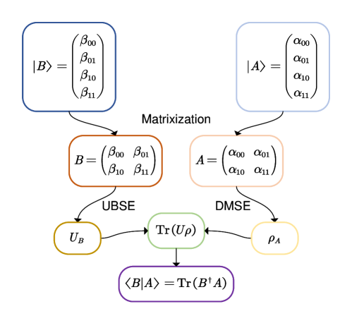
Figure 1: Sketch of the algorithm. To estimate the amplitude $\langle B|A\rangle$, we first do the matrixization procedure to convert both $|A\rangle$ and $|B\rangle$ into matrices $A$ and $B$. Then we encode $A$ into a non-diagonal block of a density matrix $\rho_{A}$ by DMSE and use UBSE to let unitary operator $U_{B}$ be a block encoding of $B$. In this way, we can further use the Hadamard test or the amplitude estimation to evaluate values of the form $\mathrm{Tr}(U\rho)$ to give an estimation of the amplitude $\langle B|A\rangle=\mathrm{Tr}(B^{\dagger}A)$.

@C=2.4em @R=1.6em & 3 3 1
1 1 0
X iY
1U_B 1U_B^† U_B
U_B U_B^†
34.8em.8emρ_A
4757.8em}

@C=2.4em @R=1.6em & H 4W_r H
H W_r H
W_r
W_r U_B
W_r
34.8em.8emρ_A
4555.8em}

@C=2.4em @R=1.6em & H 1 H
1W_r
W_r[1]
[1]
2W_r
W_r U_B
W_r
46.8em.8em—S_A⟩
6575.8em}

Figure 2: (a): The circuit diagram of $W_{r}$. For $W_{i}$, we can simply turn the $X$, $iY$, and CZ gates in $W_{r}$ into $iX$, $Y$, and $|00\rangle\langle 00|-|01\rangle\langle 01|-|10\rangle\langle 10|-|11\rangle\langle 11|$. The systems are arranged in the order $\{1,1,1,n,k\}$. (b): The circuit diagram of $U_{B,r1}$. For $U_{B,i1}$, we can simply turn $W_{r}$ to $W_{i}$. The systems are arranged in the order $\{1,1,1,n,k\}$. (c): The circuit diagram of $U_{B,r2}$. For $U_{B,i2}$, we can simply turn $W_{r}$ to $W_{i}$. The systems are arranged in the order $\{1,1,1,m,1,n,k\}$.

In this work, we consider the indirect estimation algorithm summarized in Fig. (1). Suppose that we have $2n$-qubit states $|A\rangle$ and $|B\rangle$ with the expressions $|A\rangle=\sum_{ij}\alpha_{ij}|i\rangle|j\rangle$ and $|B\rangle=\sum_{ij}\beta_{ij}|i\rangle|j\rangle$ (When this is not the case, we can always add an ancilla qubit to meet the case.), we first turn them into $n$-qubit matrices $A=\sum_{ij}\alpha_{ij}|i\rangle\langle j|$ and $B=\sum_{ij}\beta_{ij}|i\rangle\langle j|$ which we call the matrixization procedure. For example, under matrixization, a 2-qubit Bell state $(|0\rangle|0\rangle+|1\rangle|1\rangle)/\sqrt{2}$ will be turned into an un-normalized single-qubit identity operator $I/\sqrt{2}$. We will also call the inverse procedure the vectorization procedure. Their formal definitions are given below:

Definition 1 (Vectorization).

Given a matrix $O=\sum_{ij}o_{ij}|i\rangle\langle j|$, the vectorization mapping $\mathcal{V}$ has the operation:

$$\mathcal{V}[M]=\ket{\ket{O}}=\sum_{ij}o_{ij}|i\rangle|j\rangle.$$

Definition 2 (Matrixization).

Given a vector $\ket{\ket{O}}=\sum_{ij}o_{ij}|i\rangle|j\rangle$, the matrixization mapping $\mathcal{M}$ has the operation:

$$\mathcal{M}[\ket{\ket{O}}]=O=\sum_{ij}o_{ij}|i\rangle\langle j|.$$

We can also understand these two mappings from Choi–Jamiołkowski isomorphism [23].

When $|A\rangle$ and $|B\rangle$ are turned into matrices, we have $\langle B|A\rangle=\mathrm{Tr}(B^{\dagger}A)$. Thus, now the task is to find quantum objects that encode $A$ and $B$ such that the value of $\mathrm{Tr}(B^{\dagger}A)$ can be estimated. In quantum computing, we are familiar with values of the form $\mathrm{Tr}(U\rho)$ which can be evaluated by the Hadamard test or the amplitude estimation. The similarity of $\mathrm{Tr}(U\rho)$ and $\mathrm{Tr}(B^{\dagger}A)$ invokes us to encode $B$ into a unitary operator $U_{B}$ and encode $A$ into a density matrix $\rho_{A}$. In this way, we can estimate the amplitude under the matrixization picture with again the help of the Hadamard test or the amplitude estimation, and the benefit of the matrixization will be clear in the following.

II.2 Density matrix state encoding and unitary block state encoding

The main idea in this work is to encode the $2n$-qubit pure state $|B\rangle$ into a $2^{n}\times 2^{n}$ diagonal block of a $k+n$-qubit unitary operator $U_{B}$ which we call the unitary block state encoding (UBSE) and encode the $2n$-qubit pure state $|A\rangle$ into a $2^{n}\times 2^{n}$ non-diagonal block of a $l+n$-qubit density matrix $\rho_{A}$ which we call the density matrix state encoding (DMSE).

Under the vectorization and the matrixization mappings, UBSE is defined as:

Definition 3 (Unitary block state encoding (UBSE)).

Given a $n+k$-qubit unitary operator $U_{B}$, if $U_{B}$ satisfies:

$$\mathcal{V}[(I_{n}\otimes\langle 0|_{k})U_{B}(I_{n}\otimes|0\rangle_{k})]=\lambda|B\rangle.$$

where $|0\rangle_{k}$ is the all-zero computational basis of the $k$-qubit ancilla system, $\lambda\geq 0$, and $|B\rangle$ is an $2n$-qubit pure state, then $U_{B}$ is called a $(n+k,\lambda)$-UBSE of $|B\rangle$.

In other words, $U_{B}$ is a block encoding [24] of $B=\mathcal{M}[|B\rangle]$.

DMSE is defined as:

Definition 4 (Density matrix state encoding (DMSE)).

Given an $l+n$-qubit density matrix $\rho_{A}$, if $\rho_{A}$ satisfies:

$$\mathcal{V}[(\langle s_{1}|_{l}\otimes I_{n})\rho_{A}(|s_{2}\rangle_{l}\otimes I_{n})]=\gamma|A\rangle.$$

where $|s_{1}\rangle_{l}$ and $|s_{2}\rangle_{l}$ satisfying $\langle s_{1}|s_{2}\rangle_{l}=0$ are two computational basis states of the $l$-qubit ancilla system, $\gamma\geq 0$, and $|A\rangle$ is a $2n$-qubit pure state, then $\rho_{A}$ is called a $(l+n,s_{1},s_{2},\gamma)$-NDSE of $|A\rangle$.

The reason we use the non-diagonal block of density matrices is to get around the Hermitian and positive semi-definite restrictions of density matrices. In this work, we will mainly focus on $(1+n,0,1,\gamma)$-DMSE where $\rho_{A}$ has the form:

$$\rho_{A}=\begin{pmatrix}\cdot&\gamma A\\ \gamma A^{\dagger}&\cdot\end{pmatrix}.$$ (1)

Note that $\rho_{A}$ is also a $(1+n,1,0,\gamma)$-DMSE of $|A^{\dagger}\rangle$.

II.3 Estimating the amplitude

Now, we talk about the query complexity of estimating $\langle B|A\rangle$ in terms of $U_{B}$ and the preparation operation of $\rho_{A}$ (and also their conjugate transposes). The constructions of $U_{B}$ and $\rho_{A}$ will be given in the following. It is sufficient to consider only the query complexity and compare them directly with direct estimation methods since the complexity of building $U_{B}$ and preparing $\rho_{A}$ is at the same level as the complexity of preparing $|B\rangle$ and $|A\rangle$. We now give two algorithms for estimating $\langle B|A\rangle$ achieving the standard quantum limit (s.q.l.) and the Heisenberg limit (h.l.) respectively. The s.q.l. estimation requires the building of two $n+k+3$-qubit unitaries $W_{r}$ and its variant $W_{i}$ shown in Fig. (2)a to estimate $\text{Re}[\langle B|A\rangle]$ and $\text{Im}[\langle B|A\rangle]$, respectively. The first two qubits are two ancilla qubits needed for the use of linear combinations of unitaries (LCU) [25, 26]. The third qubit with the next $n$ qubits forms the system of $\rho_{A}$. The $n$ qubits with the last $k$ qubits form the system of $U_{B}$. Both $W_{r}$ and $W_{i}$ take a single query of $U_{B}$ and $U_{B}^{\dagger}$ respectively. With $W_{r}$ and $W_{i}$, we can further construct two unitaries $U_{B,r1}$ and $U_{B,i1}$ shown in Fig. (2)b such that:

$$\frac{\mathrm{Tr}(U_{B,r1}|00\rangle\langle 00|\otimes\rho_{A}\otimes|0\rangle\langle 0|_{k})}{\gamma\lambda} =\text{Re}[\langle B|A\rangle],$$ (2)

$$\frac{\mathrm{Tr}(U_{B,i1}|00\rangle\langle 00|\otimes\rho_{A}\otimes|0\rangle\langle 0|_{k})}{\gamma\lambda} =\text{Im}[\langle B|A\rangle].$$ (3)

The form of these formulas indicates we can use the Hadamard test to do the estimation with the following theorem (Appendix B):

Theorem 1a (s.q.l. estimation by state matrixization.).

Given $U_{B}$ a $(n+k,\lambda)$-UBSE of $|B\rangle$ and $\rho_{A}$ a $(1+n,0,1,\gamma)$-DMSE of $|A\rangle$, we can estimate $\mu_{r}=\text{Re}[\langle B|A\rangle]$ and $\mu_{i}=\text{Im}[\langle B|A\rangle]$ by doing the Hadamard test following Eq. (2) and Eq. (3). The query complexity to achieve a relative error $\epsilon$ (i.e. $|\overline{\mu_{r(i)}}-\mu_{r(i)}|\leq\epsilon|\mu_{r(i)}|$) with a success probability at least $1-\delta$ is:

$$T_{s}=\mathcal{O}(\gamma^{-2}\lambda^{-2}|\mu_{r(i)}|^{-2}\epsilon^{-2}\log(\delta^{-1})).$$ (4)

Thus, we can see there is $\gamma^{-2}\lambda^{-2}$ reduction on the complexity compared with the direct Hadamard test estimation.

The h.l. estimation also requires the building of $W_{r}$ and $W_{i}$, but now, we need an additional ancilla qubit (ordered at the front) and require the use of the $m+n+1$-qubit state $|S_{A}\rangle$ as the purification of $\rho_{A}$ instead of $\rho_{A}$. With $W_{r}$ and $W_{i}$, inspired by the construction in Ref. [27], we can build two $m+n+k+4$-qubit unitaries $U_{B,r2}$ and $U_{B,i2}$ as shown in Fig. (2)c such that:

$$\frac{2|\langle 000|\langle S_{A}|\langle 0|_{k}U_{B,r2}|0\rangle_{k}|S_{A}\rangle|000\rangle|-1}{\gamma\lambda} =\text{Re}[\langle B|A\rangle],$$ (5)

$$\frac{2|\langle 000|\langle S_{A}|\langle 0|_{k}U_{B,i2}|0\rangle_{k}|S_{A}\rangle|000\rangle|-1}{\gamma\lambda} =\text{Im}[\langle B|A\rangle].$$ (6)

The form of these formulas indicates we can use the amplitude estimation algorithm to do the estimation by building the Grover operators $U_{G,r(i)}=-(I-2U_{B,r2(i2)}|0S_{A}0\rangle\langle 0S_{A}0|U_{B,r2(i2)}^{\dagger})(I-2|0S_{A}0\rangle\langle 0S_{A}0|)$ with $|0S_{A}0\rangle$ short for $|0\rangle_{k}|S_{A}\rangle|000\rangle$. In each $U_{G,r(i)}$, we have 2 queries on $U_{B}$, $U_{B}^{\dagger}$, $U_{SA}$, and $U_{SA}^{\dagger}$ with $U_{SA}|0\rangle_{m+1+n}=|S_{A}\rangle$. Here, we can use modified versions of amplitude estimation [11, 12] avoiding the use of quantum Fourier transform. The whole procedure supports the following theorem (Appendix B):

Theorem 1b (h.l. estimation by state matrixization.).

Given $U_{B}$ a $(n+k,\lambda)$-UBSE of $|B\rangle$ and $|S_{A}\rangle$ a $(1+n,0,1,\gamma)$-DMSE of $|A\rangle$, we can estimate $\mu_{r}=\text{Re}[\langle B|A\rangle]$ and $\mu_{i}=\text{Im}[\langle B|A\rangle]$ by doing the amplitude estimation following Eq. (5) and Eq. (6). The query complexity to achieve a relative error $\epsilon$ with a success probability at least $1-\delta$ is:

$$T_{h}=\mathcal{O}(\gamma^{-1}\lambda^{-1}|\mu_{r(i)}|^{-1}\epsilon^{-1}\log(\delta^{-1})).$$ (7)

Thus, we can see there is $\gamma^{-1}\lambda^{-1}$ reduction on the complexity compared with the direct amplitude estimation. Note that while direct amplitude estimation can only estimate $|\langle A|B\rangle|$, it is easy to modify it to be able to also estimate $\text{Re(Im)}[\langle A|B\rangle]$ [27].

One thing to mention is that the exact values of $\lambda$ and $\gamma$ can be directly concluded from the ways of the construction of $U_{B}$ and the preparation of $\rho_{A}$ shown in the following. Nevertheless, for completeness, we also give measurement strategies in the Appendix B.3 when their values can not be known in prior.

II.4 Construction of $U_{B}$

Now we consider the construction of $U_{B}$ and $\rho_{A}$. For the state $|B\rangle$, since its form is already known, we can thus easily know the form of $B$, and we can use the well-developed techniques of block encoding [26] to build $U_{B}$. Here, due to the restriction of unitarity of $U_{B}$ and the equivalence between the Schmidt decomposition of $|B\rangle$ and the singular value transformation of $B$, we can set the relations between the upper bound of $\lambda$ and the entanglement of $|B\rangle$ between the first $n$-qubit subsystem called the upper subsystem (US) and the last $n$-qubit subsystem called the lower subsystem (LS):

Theorem 2a (Upper bound on $\lambda$).

Given a state $|B\rangle$, the value of $\lambda$ in $U_{B}$ has the upper bound:

$$\lambda\leq\frac{1}{\|B\|_{\infty}}=2^{\frac{H_{\infty}(|B\rangle)}{2}},$$

where $\|\cdot\|_{\infty}$ is the spectral norm (largest singular values) and $H_{\infty}(|B\rangle)=-\log_{2}(\max_{i}\beta_{i}^{2})$ is the $\infty$-Rényi entropy [28] of $|B\rangle$ under the partition between US and LS.

Thus, $|B\rangle$ with larger entanglement has larger achievable $\lambda$. For example, when $|B\rangle=|\psi_{1}\rangle|\psi_{2}\rangle$ is a product state, $\lambda$ has the smallst value $1$. On the other hand, when $|B\rangle$ is a maximally entangled state, $B$ will be an un-normalized unitary operator and we can directly use this unitary operator as $U_{B}$ with the largest $\lambda=2^{n/2}$. For $U_{B}$, we have $\|U_{B}\|_{\infty}=1$ while for $|B\rangle$, we have the vector 2-norm $\||B\rangle\|_{2}=1$. It is this difference between the norm restrictions that gives possible improvements (large $\lambda$) of our method.

When $|B\rangle$ can be expressed as a small number of linear combinations of maximally entangled states:

$$|B\rangle=\sum_{i=1}^{2^{k}}c_{i}|v_{i}\rangle,$$ (8)

and we know this decomposition priorly, large values of $\lambda$ can be achieved. We can use LCU to construct a $n+k$-qubit unitary $U_{B}$ with $\lambda=2^{n/2}\||B\rangle\|_{1}^{-1}$ where $\||B\rangle\|_{1}=\sum_{i=1}^{2^{k}}|c_{i}|\leq 2^{k/2}$ denotes the vector 1-norm of $|B\rangle$. The complexity of constructing $U_{B}$ is also at the same level as preparing $|B\rangle$ [29]. Here, we only consider a restricted model of UBSE. It would be interesting to see if other block encoding methods [24, 30] will lead to more efficient UBSE protocols and get benefits from other access models beyond Eq. (8). We want to mention that it is possible to use the methods in Ref. [31, 32] to construct $U_{B}$ for any $|B\rangle$ even if it is prepared by complicated quantum operations, however, this can only give $\lambda=1$ leading to no advantage of our method.

II.5 Preparation of $\rho_{A}$

We now show how to prepare $\rho_{A}$. For its purification $|S_{A}\rangle$, we can always use the Stinespring dilation [33] to find its corresponding preparations. Similar to the case of $U_{B}$, $\gamma$ has an upper bound decided by the entanglement of $|A\rangle$:

Theorem 2b (Upper bound on $\gamma$).

Given a state $|A\rangle$, the value of $\gamma$ in $\rho_{A}$ has the upper bound:

$$\gamma\leq\frac{1}{2\|A\|_{1}}=2^{-\frac{H_{1/2}(|A\rangle)}{2}-1},$$

where $\|\cdot\|_{1}$ is the trace norm (sum of singular values) and $H_{1/2}(|A\rangle):=2\log_{2}(\sum_{i}\alpha_{i})$ is the $1/2$-Rényi entropy of $|A\rangle$ under the partition between US and LS.

Contrary to $\lambda$, this theorem implies that $|A\rangle$ with larger entanglement has smaller achievable $\gamma$. For example, when $|A\rangle=|\psi_{1}\rangle|\psi_{2}\rangle$ is a product state, we can let $\rho_{A}=1/2(|0\rangle|\psi_{1}\rangle+|1\rangle|\psi_{2}^{*}\rangle)(\langle 0|\langle\psi_{1}|+\langle 1|\langle\psi_{2}^{*}|)$ to obtain the largest $\gamma=1/2$. When $A=2^{-n/2}I$ corresponds to $|A\rangle$ a maximally entangled state, we can let $\rho_{A}=2^{-n}|+\rangle\langle+|\otimes I$ such that $\gamma=2^{-n/2-1}$ achieving the smallest upper bound. In fact, for any $|A\rangle$, we can give its optimal construction based on the Schmidt decomposition of $|A\rangle$ (see Appendix C.1).

In most cases, $|A\rangle$ is prepared by a complicated quantum operation from an initial product state $|A_{0}\rangle$. Thus, we have little knowledge of the Schmidt decomposition of $|A\rangle$ and cannot prepare $\rho_{A}$ similar to the way of $U_{B}$. To address this issue, the correct workflow is to convert this operation into the matrixization picture and act it on $\rho_{A_{0}}$ to prepare $\rho_{A}$. This leads to a new technique which we call channel block encoding (CBE). We consider applying a quantum channel $\mathcal{C}[\cdot]$ to $\rho_{A_{0}}$ with the form:

$$\mathcal{C}[\rho_{A_{0}}]=\sum_{i}\begin{pmatrix}K_{i}&0\\ 0&L_{i}\end{pmatrix}\rho_{A_{0}}\begin{pmatrix}K_{i}^{\dagger}&0\\ 0&L_{i}^{\dagger}\end{pmatrix},$$ (9)

where $\{K_{i}\}$ and $\{L_{i}\}$ are two sets of Kraus operators satisfying $\sum_{i}K_{i}^{\dagger}K_{i}=\sum_{i}L_{i}^{\dagger}L_{i}=I_{n}$. Focusing on the upper right block $\rho_{A_{0}}$, we equivalently build the operation in the vectorization picture:

$$\gamma_{0}|A_{0}\rangle\rightarrow\gamma_{0}\sum_{i}K_{i}\otimes L_{i}^{*}|A_{0}\rangle.$$ (10)

It can be proved that $\sum_{i}K_{i}\otimes L_{i}^{*}$ is universal to encode arbitrary operators (see Appendix C.2). Now, what we need to do is to adjust $\{K_{i}\}$ and $\{L_{i}\}$ such that $\sum_{i}K_{i}\otimes L_{i}^{*}$ encodes the quantum operation. The formal definition is shown below:

Definition 5 (Channel block encoding (CBE)).

Given a $2n$-qubit operator $O$, if we can find a $l+n$-qubit quantum channel of the form Eq. (9) whose matrix form $C$ satisfies the condition:

$$\|\eta O-(\langle s|\otimes I)C(|s\rangle\otimes I)\|\leq\varepsilon,$$

with the encoding efficiency $\eta\geq 0$, $s$ a binary string and $|s\rangle$ a $l$-qubit computational basis, then the channel is a $(l+n,s,\eta,\varepsilon)$-CBE of $O$.

With the help of CBE, we can therefore build various operations. Here, we consider $|A\rangle$ is prepared by a unitary operator $V$ such as a quantum circuit or a Hamiltonian simulation from $|A_{0}\rangle$. But we want to emphasize that since there are no unitary restrictions on $\sum_{i}K_{i}\otimes L_{i}^{*}$, one can also try to build nonphysical operations such as imaginary time evolution [34] and deterministic POVMs [33]. Suppose we have a CBE of $V$ with an efficiency $\eta_{v}$, then we must have $\gamma=\eta_{v}\gamma_{0}$. Thus, we expect $\eta_{v}$ to be as large as possible, however, since both $\gamma$ and $\gamma_{0}$ have upper bounds decided by $|A\rangle$ and $|A_{0}\rangle$, there is also an upper bound for $\eta_{v}$ of $V$ by the following corollary:

Corollary 1 (Upper bound on $\eta_{v}$ for unitary operators).

Given a unitary $V$, the value of $\eta_{v}$ in CBE of $V$ has the upper bound:

$$\eta_{v}\leq 2^{-\frac{H_{1/2}(V)}{2}},$$

where $H_{1/2}(V)$ is defined as $H_{1/2}(V):=\sup_{|\psi\rangle}|H_{1/2}(V|\psi\rangle)-H_{1/2}(|\psi\rangle)|$.

Here, $|\psi\rangle$ in $H_{1/2}(V)$ is defined allowing local ancilla qubits and initial entanglement of $|\psi\rangle$ [35]. Therefore, the upper bound of $\eta_{v}$ is connected with the power of entanglement generation of $V$. Since $\gamma=\eta_{v}\gamma_{0}\leq\eta_{v}/2$, we require the entanglement power of $V$ to be relatively small to make $\gamma$ large. Note that this corollary only restricts the entanglement power of $V$ between the US and LS but does not restrict its power inside the US and LS.

We can construct optimal CBE for quantum circuits and Hamiltonian simulations in terms of individual single-qubit/two-qubit gates and Trotter steps. Since we regard each gate/Trotter step as a channel, the complexity of preparing $\rho_{A}$ is thus at the same level as preparing $|A\rangle$. Note that when a gate or a Trotter step has no interaction between US and LS, we have their CBE efficiency equal to 1, thus, we only need to consider those interaction terms. To achieve the optimal construction for interaction terms, we can use the following channel $\mathcal{C}_{G}[\cdot]$

$$\mathcal{C}_{G}[\rho] =\frac{s_{i}}{s_{i}+s_{x}+s_{y}+s_{z}}\begin{pmatrix}e^{i\phi_{i}}I&0\\ 0&I\end{pmatrix}\rho\begin{pmatrix}e^{-i\phi_{i}}I&0\\ 0&I\end{pmatrix}$$ (11)

$$+\frac{s_{x}}{s_{i}+s_{x}+s_{y}+s_{z}}\begin{pmatrix}e^{i\phi_{x}}X&0\\ 0&X\end{pmatrix}\rho\begin{pmatrix}e^{-i\phi_{x}}X&0\\ 0&X\end{pmatrix}$$

$$+\frac{s_{y}}{s_{i}+s_{x}+s_{y}+s_{z}}\begin{pmatrix}e^{i\phi_{y}}Y&0\\ 0&-Y\end{pmatrix}\rho\begin{pmatrix}e^{-i\phi_{y}}Y&0\\ 0&-Y\end{pmatrix}$$

$$+\frac{s_{z}}{s_{i}+s_{x}+s_{y}+s_{z}}\begin{pmatrix}e^{i\phi_{z}}Z&0\\ 0&Z\end{pmatrix}\rho\begin{pmatrix}e^{-i\phi_{z}}Z&0\\ 0&Z\end{pmatrix},$$

to encode any 2-qubit unitary operators $G$ connecting US and LS that have the canonical form [36]:

$$G=e^{i(\theta_{x}X\otimes X+\theta_{y}Y\otimes Y+\theta_{z}Z\otimes Z)}=s_{i}e^{i\phi_{i}}I\otimes I+s_{x}e^{i\phi_{x}}X\otimes X+s_{y}e^{i\phi_{y}}Y\otimes Y+s_{z}e^{i\phi_{z}}Z\otimes Z,$$ (12)

with an efficiency $\eta_{G}=1/(s_{i}+s_{x}+s_{y}+s_{z})$. Here, $s_{i}$, $s_{x}$, $s_{y}$ and $s_{z}$ are positive numbers. $\eta_{G}$ can be proved to achieve the upper bound in Corollary 1 (see Appendix C.3).

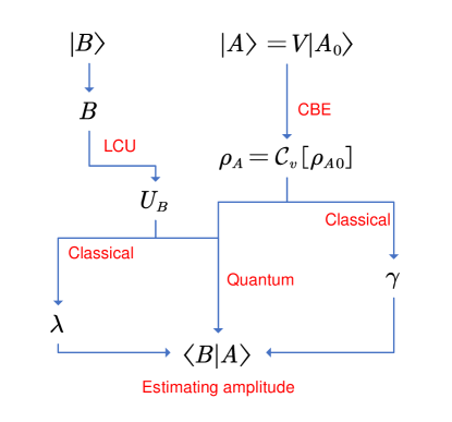
Figure 3: Workflow of the algorithm. To estimate the amplitude $\langle B|A\rangle$, we need to construct $U_{B}$ and prepare $\rho_{A}$. For $U_{B}$, we first turn $|B\rangle$ of the form Eq. (8) into its matrix form and then use LCU to do the block encoding of $B$ to obtain $U_{B}$. Since the form of $|B\rangle$ is known priorly, the value of $\lambda=2^{n/2}\||B\rangle\|_{1}^{-1}$ can be directly calculated from the way of the LCU construction. For $\rho_{A}$, we know $|A\rangle=V|A_{0}\rangle$, thus, we need to first prepare $\rho_{A_{0}}$ and construct a channel $\mathcal{C}_{v}[\cdot]$ as the CBE of $V$, then we can prepare $\rho_{A}=\mathcal{C}_{v}[\rho_{A_{0}}]$. Since we can easily calculate the CBE efficiency of $V$ from its construction, the value of $\gamma$ can also be known directly. Now, we can use these elements with the Hadamard test to give a s.q.l. estimation of the amplitude $\langle B|A\rangle$ based on Eq. (2) and Eq. (3), and with the amplitude estimation to give a h.l. estimation of the amplitude $\langle B|A\rangle$ based on Eq. (5) and Eq. (6).. Note that for h.l. estimation, we need to use $|S_{A}\rangle$ instead of $\rho_{A}$.

Since any two-qubit gates are locally equivalent to the above canonical form, their CBE constructions based on Eq. (11) are also optimal. For example, a CNOT gate has an optimal CBE efficiency $1/\sqrt{2}$. For Hamiltonian simulations by the product formula, if each interacting term between US and LS in the Hamiltonian is a Pauli operator (having $\{X,Y,Z\}$ on both US and LS), the corresponding Trotter step is also equivalent under local Clifford circuits to a canonical form, thus, the CBE construction of each Trotter step based on Eq. (11) is also optimal. Now, since we know the CBE efficiency of each component, the CBE efficiency of the whole circuit or the dynamics evolution and the value of $\gamma$ can be easily calculated. Based on these constructions, we have the following theorem:

Theorem 3a (CBE of quantum circuit).

Suppose we have $|A\rangle=V|A_{0}\rangle$ with $|A_{0}\rangle$ as a product state between US and LS with the largest $\gamma_{0}=1/2$ and $V$ is a quantum circuit with $K$ CNOT gates connecting US and LS, then $\rho_{A}$ can be prepared by acting a channel on $\rho_{A0}$ such that $\gamma$ in $\rho_{A}$ satisfies:

$$\gamma=2^{-1-K/2}.$$

Theorem 3b (CBE of Hamiltonian simulation by the first-order product formula).

Suppose we have $|A\rangle=V|A_{0}\rangle$ with $|A_{0}\rangle$ a product state between US and LS with the largest $\gamma_{0}=1/2$ and $V\approx e^{-iHt}$ is the first-order product formula approximation of the dynamics governed by a Hamiltonian $H=\sum_{i}h_{i}P_{i}$ with $\|H\|_{\text{Inter}}:=\sum_{i\in\text{Inter}}|h_{i}|$ containing only interaction terms, then $\rho_{A}$ can be prepared by acting a channel on $\rho_{A0}$ such that $\gamma$ in $\rho_{A}$ satisfies:

$$\gamma\approx 2^{-1}e^{-\|H\|_{\text{Inter}}t}.$$

Here, in Theorem 3a, we use the number of CNOT gates as a benchmark since it is a standard gate in many universal gate sets. In Theorem 3b, we consider only the first-order product formula [37] for simplicity, nevertheless, the lower bound should be nearly tight and cannot be optimized by high-order product formulas [38] and other simulation methods such as LCU [39] and QSP [40] as it matches the direct implementation of $e^{-iHt}$ when we assume a sufficiently large Trotter steps for the proof (See Appendix C.4). We want to emphasize that in practice, one can use various group strategies to optimize the encoding efficiency in Theorem 3a and 3b. For example, a SWAP gate has its optimal CBE encoding efficiency $1/2$, but if one trivially uses 3 CBE channels of CNOT to build the SWAP gate, the efficiency will be only $2^{-3/2}$.

Now, we can summarize the whole workflow of our algorithm in Fig. (3).

III Improvements on estimating amplitudes

The interesting point of our method is that we compress $2n$-qubit information in $n$-qubit systems, but this can surprisingly give benefits: we can estimate the amplitude $\langle B|A\rangle$ with complexity reductions $\gamma^{-2}\lambda^{-2}$ and $\gamma^{-1}\lambda^{-1}$ in Eq. (4) and (7) compared with direct estimations by Hadamard tests and amplitude estimations. The improvement is more significant with a larger $\gamma\lambda$. In an extreme case where $|A\rangle$ is a product state between US and LS and $|B\rangle$ is a maximally entangled state between US and LS, we are allowed to have the largest value $\gamma\lambda=2^{n/2-1}$ with $\gamma=1/2$ and $\lambda=2^{n/2}$, which is an exponential improvement over traditional methods. In this case, we summarize the query complexity requirements to estimate the amplitude to a relative error $\epsilon=\mathcal{O}(1)$ in Table 1.

Amplitude	Direct estimation (s.q.l.)	Direct estimation (h.l.)	Our method (s.q.l.)	Our method (h.l.)
$\mathcal{O}(2^{-n/2})$	$\mathcal{O}(2^{n})$	$\mathcal{O}(2^{n/2})$	$\mathcal{O}(1)$	$\mathcal{O}(1)$
$\mathcal{O}(2^{-n})$	$\mathcal{O}(2^{2n})$	$\mathcal{O}(2^{n})$	$\mathcal{O}(2^{n})$	$\mathcal{O}(2^{n/2})$

Table 1: Comparisons of query complexities for a $\epsilon=\mathcal{O}(1)$-relative estimation of $\langle B|A\rangle$. We consider the extreme cases where $|A\rangle$ is a product state between US and LS and has been encoded into $\rho_{A}$ achieving the upper bound in Theorem 2b, and $|B\rangle$ is a maximally entangled state between US and LS and has been encoded into $U_{B}$ achieving the upper bound in Theorem 2a. We consider two scenarios: $\text{Re(Im)}[\langle B|A\rangle]$ is of order $\mathcal{O}(2^{-n/2})$ and is of order $\mathcal{O}(2^{-n})$, which are related with discussions in the implication section.

Thus, we can see that when $\text{Re(Im)}[\langle B|A\rangle]$ is of order $\mathcal{O}(2^{-n/2})$, we can achieve an exponential speedup over traditional methods. Since we are considering $2n$-qubit systems, this corresponds to situations where $|A\rangle$ is relatively concentrated on $|B\rangle$. When $\text{Re(Im)}[\langle B|A\rangle]$ is of order $\mathcal{O}(2^{-n})$ which is the cases where $|A\rangle$ is anti-concentrated on $|B\rangle$, we can achieve a complexity using only a standard quantum limit estimation (Eq. (2)-(3)) comparable with the direct estimation (h.l.), which also means we can achieve an equivalent quadratic speedup over the direct estimation (s.q.l.) without changing the dependence on $\epsilon$. Moreover, in this example, by using the Heisenberg limit estimation (Eq. (5)-(6)), we can even achieve an equivalent quadratic speedup over the direct estimation (h.l.) and an equivalent quartic speedup over the direct estimation (s.q.l.). Note that we are not actually achieving for example the truly quartic speedup with respect to $\epsilon$ i.e. $\epsilon^{-1/2}$, but only having the value $\gamma\lambda$ reduce the complexity and enable a quartic speedup in total performance.

	$\mathcal{O}(1)\sim\mathcal{O}(\log(n))$	$\mathcal{O}(\text{poly}\log(n))$
$\mathcal{O}(1)\sim\mathcal{O}(\text{poly}(n))$	exponential	superpolynomial
$\mathcal{O}(\exp(\text{poly}\log(n)))$	superpolynomial	superpolynomial

Table 2: The value of $\gamma\lambda$ in various regimes. Here, $\||B\rangle\|_{1}=\sum_{i=1}^{2^{k}}|c_{i}|$ denotes the vector 1-norm of $|B\rangle$ under the unitary decomposition Eq. (8). The depth denotes the number of CNOT gates connecting US and LS (Theorem 3a) and the simulation time denotes $\|H\|_{\text{Inter}}t$ (Theorem 3b). $|A\rangle$ is obtained by acting a quantum circuit of such a depth or a Hamiltonian simulation of such a time on an initial product state $|A_{0}\rangle$. Here, ”exponential”, ”superpolynomial”, and ”polynomial” are with respect to $n$.

In practical scenarios, both $|A\rangle$ and $|B\rangle$ can deviate from the above extreme case, making the improvement $\gamma\lambda$ much milder. Also, when we consider the general setting where we use CBE to prepare $\rho_{A}$ (Theorem 3a and 3b) and use LCU to prepare $U_{B}$ with $|B\rangle$ obeying the form of Eq. (8), the value of $\gamma\lambda$ can be further reduced. When the entanglement of $|B\rangle$ is too small and the depth or the Hamiltonian simulation time in $V$ is too big, our algorithm can only have mild advantages or even disadvantages over direct estimation methods. In Table 2, we summarize the value of $\gamma\lambda$ in various regimes. Thus, we require the quantum circuit depth (number of CNOT gates connecting US and LS) or the Hamiltonian simulation time ($\|H\|_{\text{Inter}}t$) to be no larger than $\mathcal{O}(\text{poly}\log(n))$ and $\||B\rangle\|_{1}$ the vector 1-norm of $|B\rangle$ to be no larger than $\mathcal{O}(\exp(\text{poly}\log(n)))$ to have at least a superpolynomial improvement (the value of $\gamma\lambda$) on estimating amplitudes. Such a regime is of particular interest which we will discuss in the following section.

IV Implications and applications

IV.1 $|A\rangle$ as a product state

When $|A\rangle=|A_{u}\rangle|A_{l}\rangle$ is a product state between US and LS, we can achieve the largest value of $\gamma=1/2$. For such $|A\rangle$, while there is no entanglement between US and LS, the entanglement within US and LS respectively has no restrictions and thus $|A\rangle$ can easily become classically intractable. Also, since we generally require $|B\rangle$ to have a large entanglement between US and LS, estimating $\langle B|A\rangle$ is intrinsically a $2n$-qubit problem despite $|A\rangle$ as a product state and thus can not be efficiently turned down to $n$-qubit systems by circuit cutting methods [41, 42].

BQP-completeness: If we have $|A\rangle=|A_{u}\rangle|A_{u}^{*}\rangle$ with $|A_{u}\rangle$ an arbitrary $n$-qubit state and set $|B\rangle=|B_{b}\rangle$ a Bell basis state, then we have $\langle B|A\rangle=2^{-n/2}\langle A_{u}|P|A_{u}\rangle$ with $P$ a $n$-qubit Pauli operator (Here, $A=|A_{u}\rangle\langle A_{u}|$). It is known that estimating the Pauli expectation value up to a (polynomial) small additive error is BQP-complete [43, 44] and the essence of our method is to use $\langle A_{u}|P|A_{u}\rangle$ to estimate $\langle B|A\rangle$ to a small relative error. When $\langle B|A\rangle$ is of order $\mathcal{O}(2^{-n/2})$, this relative error directly corresponds to the small additive error of estimating Pauli expectation values, and thus the whole setup is also BQP-complete. This also indicates that the efficient estimation of $\mathcal{O}(2^{-n/2})$ amplitudes is the best we can expect and it is beyond the capability of quantum computers for smaller amplitudes such as those of order $\mathcal{O}(2^{-n})$.

Bell sampling: Recently, there have been various protocols ranging from quantum learning [45, 46] to quantum advantage experiments [47] based on the setup where we have $|A\rangle=|A_{u}\rangle|A_{u}\rangle$ with $|A_{u}\rangle$ an arbitrary $n$-qubit state and set $|B\rangle=|B_{b}\rangle$ a Bell basis state. In Ref. [47], the authors propose the Bell sampling protocol and show that we can encode any GapP functions into the amplitude $\langle B|A\rangle$. Since estimating $\langle B|A\rangle$ to a small relative error corresponds to estimating the values of the GapP functions to a small relative error which is GapP-hard [3], our method is unlikely to be able to efficiently estimate such amplitudes, otherwise, we would have quantum computers to be able to solve problems over the entire polynomial hierarchy [48]. This also indicates that such amplitudes should be exponentially smaller than $\mathcal{O}(2^{-n/2})$ such that the resulting complexity of our method is still exponential, which is true for most quantum advantage protocols where the anti-concentration effect [49, 3] makes almost all amplitudes around $\mathcal{O}(2^{-n})$.

IV.2 Hardness of $|B\rangle$

In the above, we have shown that if $B$ is proportional to a unitary operator $U_{B}$, then this unitary operator is exactly a UBSE of $B$ with the largest $\lambda=2^{n/2}$. If we further set $|A\rangle=|A_{u}\rangle|A_{l}\rangle$, then we have $\langle B|A\rangle=\langle A_{l}^{*}|U_{B}^{\dagger}|A_{u}\rangle$. Since $U_{B}$ can be an arbitrary unitary operator, we can even set $|A\rangle=|0\rangle|0\rangle$ and still encode any GapP functions into the amplitude $\langle B|A\rangle$ [3]. Thus, the argument is similar to the above discussions on Bell sampling.

We can also consider the random behaviors of $B$ and $|B\rangle$. To make $lambda$ large, we hope $|B\rangle$ is close to a maximally entangled state between US and LS, which is almost always true if $|B\rangle$ is picked from a state 2-design [50] since the average purity of the reduced density matrix of $|B\rangle$ is $2^{n+1}/(2^{2n}+1)\approx 2^{-n}$. Since when $B$ is proportional to a unitary operator, $|B\rangle$ is exactly a maximally entangled state, thus, a natural guess is that the randomness of $B$ can be inherited by $|B\rangle$. Indeed, we prove that when the $n$-qubit operator $U_{B}$ is drawn from a unitary 2-design, the ensemble $\{|B\rangle=2^{-n/2}\ket{\ket{U_{B}}}\}$ forms an $\mathcal{O}(2^{-2n})$-approximate $2n$-qubit state 2-design in terms of the trace distance in Appendix E.1. Since 2-design is a sufficient condition for the anti-concentration effect, the amplitudes under this setting are on average of order $\mathcal{O}(2^{-2n})$.

IV.3 $|A\rangle$ as a weakly entangled state

When $|A\rangle$ is prepared by a shallow quantum circuit or a short-time Hamiltonian simulation of depth (time) of order $\mathcal{O}(\text{poly}\log(n))$, $\gamma\lambda$ can be at best a superpolynomial large value $2^{n/2-\mathcal{O}(\text{poly}\log(n))}$ for $B$ proportional to a unitary operator. This regime is interesting because we can see this setup as a genuine $2n$-qubit setup. When $|A\rangle$ is a product state, while the large entanglement in $|B\rangle$ ensures the amplitude is a $2n$-qubit amplitude, we can see from above that we can use matrixization to convert it into a $n$-qubit value. Thus, the exponential improvement of our method can be seen as finding a way or a picture to turn these amplitudes into what they really are in terms of hardness. In other words, they are essentially $n$-qubit values but hidden in $2n$-qubit amplitudes.

However, this $2n$ to $n$ conversion doesn’t hold for weakly entangled states. This can be understood from four points. First, from the tensor network picture, the circuit or the Hamiltonian simulation has a superpolynomial large bond dimension of order $2^{\mathcal{O}(\text{poly}\log(n))}$ which is beyond the efficiently separable regime [51, 42]. Second, due to the interactions between US and LS, we can no longer use matrixization to convert it into a straightforward $n$-qubit value as in the above two cases. Third, when $|B\rangle$ is a stabilizer state, the amplitudes can be understood as the amplitudes of states prepared by Clifford circuits with non-stabilizer inputs projecting on the computational basis [52, 53]. Fourth, $\mathcal{O}(\text{poly}\log(n))$-depth/simulation time is already enough for the emergence of various interesting things such as the approximate unitary design [54], pseudorandom unitaries [54], anti-concentration [49], and quantum advantage [55, 54, 49, 56]. (Here, we assume the depths within the US and LS are at the same level of $\mathcal{O}(\text{poly}\log(n))$.) Note that for the quantum advantage claim, we typically set $|B\rangle$ as a product state (a computational basis state) which is different from our setting. Thus, further study of strict classical hardness is required. One observation on why the claim should hold is that when $|B\rangle$ is a Bell basis state, it is still a $n$-party product state of qudits.

Thus, this weakly entangled case is a genuine $2n$-qubit setup, and our method may be able to truly give a superpolynomial improvement over previous methods. This doesn’t violate the no-go theorem set by the linearity of quantum mechanics [16, 17, 18] since to build CBE for $V$, we need additional information about how $V$ is constructed rather than a black box. Even though, to the best of our knowledge, there are no known results utilizing this additional information to go beyond quadratic speedup (direct estimation, h.l.). Our method can achieve this because the logic of our method is not to directly estimate $\langle B|A\rangle$ but to first convert $|A\rangle$ and $|B\rangle$ into other objects by DMSE and UBSE and then do the estimation. For this setup, it would be interesting to see what information can we encode to amplitudes of what orders, as amplitudes of order $\mathcal{O}(2^{-n})$, $\mathcal{O}(2^{-n/2})$, and $2^{-n/2+\mathcal{O}(\text{poly}\log(n))}$ can have complexity separations in our method.

IV.4 Probing properties of low-temperature Gibbs states from high-temperature ones

An interesting implication of the state matrixization picture is that we can probe certain properties of low-temperature Gibbs states from high-temperature ones. The motivation is that $|A\rangle$ and $\rho_{A}$ are essentially different states, thus, there may exist a complexity separation in terms of the preparation of $|A\rangle$ and $\rho_{A}$. Indeed, if $\rho_{A}$ is prepared by CBE, we have shown its preparation cost is at the same level as $|A\rangle$, however, for Gibbs state, we can instead prepare $\rho_{A}$ without CBE. The reason is because the $n$-qubit Gibbs state $\rho_{\beta}=\frac{e^{-\beta H}}{\mathrm{Tr}(e^{-\beta H})}$ is exactly a DMSE of the purified Gibbs state of $\rho_{2\beta}$. Now suppose we want to probe properties such as $\langle B|\rho_{\beta}\rangle$ with $|\rho_{\beta}\rangle$ denotes the normalized vectorized state from $\rho_{\beta}$, in the traditional method, we need to actually prepare $|\rho_{\beta}\rangle$ which corresponds to the preparation of the Gibbs state at the temperature $1/(2\beta)$ which can be hard for quantum computers [57, 58], in contrast, using our method, we only need to prepare a Gibbs state at the higher temperature $1/\beta$ which can be easy for quantum computers [59]. In Appendix E.2, we give an example where the query complexity of estimating $\langle B|\rho_{\beta}\rangle$ is comparable for both methods but there can be an exponential separation on the preparation complexity between $\rho_{\beta}$ and $\rho_{2\beta}$.

V Summary and outlook

In this work, we show that by encoding the information of the states $|A\rangle$ and $|B\rangle$ into different quantum objects $\rho_{A}$ and $U_{B}$, we can reduce the complexity on estimating the quantum amplitude $\langle A|B\rangle$. We give concrete procedures to construct $U_{B}$ and prepare $\rho_{A}$ and show how to use them to give a standard quantum limit estimation and a Heisenberg limit estimation respectively. Especially, for $\rho_{A}$, we introduce channel block encoding to encode quantum operations into quantum channels under the vectorization picture. We give optimal channel block encoding constructions for gate-based quantum circuits and Hamiltonian simulations based on the product formula. The level of improvement depends on the value of $\gamma\lambda$ and we give a comprehensive discussion on different improvement regimes and their implications. We hope this work can invoke other indirect estimation protocols, lead discoveries to other quantum applications based on the state matrixization beyond this work and Ref. [21, 22], and give new possibilities for quantum algorithms.

There are several open questions and further directions we think are interesting and important. First, if we have a density matrix $\rho_{A}$ with an encoding efficiency $\gamma$ far below the upper bound, can we efficiently amplify it to the upper bound (maybe with the aid of non-unital channels)? Second, in many situations, we may want to estimate the amplitude of an unknown quantum state with a large entanglement projected on a known product state. Thus, can we change the role between $|A\rangle$ and $|B\rangle$. In other words, if $|A\rangle$ is priorly known and $|B\rangle$ is prepared by a quantum circuit, can we efficiently construct $U_{B}$ with $\lambda$ close to the upper bound? Third, invoked by the above discussions of the weakly entangled regime, can we rigorously encode $\#$P instances into amplitudes that fit our algorithm and show more than quadratic quantum speedup compared with classical counterparts? Fourth, what’s the potential of using channel block encoding to implement non-physical operations such as imaginary time evolution [34] and deterministic POVMs [33] for more applications?

Appendix A Preliminary: Hadamard test and amplitude estimation

Given a unitary $U$ and a density matrix $\rho$, Hadamard test [10] can give a standard quantum limit estimate of $\text{Re}[\mathrm{Tr}(U\rho)]$ by measuring the Pauli $Z$ expectation value of an ancilla qubit. Assuming $|\text{Re}[\mathrm{Tr}(U\rho)]|\ll 1$, we have the following lemma:

Lemma 1 (Hadamard test [10]).

To estimate $\mu=\text{Re}[\mathrm{Tr}(U\rho)]$ up to a relative error $\epsilon$ (i.e. $|\bar{\mu}-\mu|\leq\epsilon|\mu|$) with a success probability at least $1-\delta$, the time (sampling) complexity is:

$$T=\mathcal{O}(|\mu|^{-2}\epsilon^{-2}\log(\delta^{-1})).$$

This lemma is derived from Hoeffding’s inequality [60] and is tight whenever $|\text{Re}[\mathrm{Tr}(U\rho)]|\ll 1$ corresponds to the case where the variance is comparable with the bound of the random variable ($\langle Z\rangle$).

Given two state $|S_{1}\rangle$ and $|S_{2}\rangle$, amplitude estimation [2, 11, 12] can give a Heisenberg limit estimate of $|\langle S_{2}|S_{1}\rangle|$ given access on the Grover operator [61]:

$$U_{G}=-(I-2|S_{1}\rangle\langle S_{1}|)(I-2|S_{2}\rangle\langle S_{2}|).$$ (13)

We have the following lemma:

Lemma 2 (Amplitude estimation [11, 12]).

To estimate $\mu=|\langle S_{2}|S_{1}\rangle|$ up to an additive error $\epsilon$ (i.e. $|\bar{\mu}-\mu|\leq\epsilon$) with a success probability at least $1-\delta$, the time complexity is:

$$T=\mathcal{O}(\epsilon^{-1}\log(\delta^{-1})).$$

Note that Lemma 2 adopts the results from Ref. [11, 12] where there is no need to build quantum Fourier transform circuit as shown in the original amplitude estimation protocol [2].

Appendix B Estimating amplitudes by DMSE and UBSE (Theorem 1a and 1b)

Given the two quantum states $|A\rangle$ and $|B\rangle$, in this work, we are interested in estimating $\langle B|A\rangle$, the amplitude of the state $|A\rangle$ on the basis state $|B\rangle$. Throughout this work, we set $|A\rangle$ and $|B\rangle$ as $2n$-qubit states. We define the first $n$-qubit subsystem as the upper subsystem (US) and the last $n$-qubit subsystem as the lower subsystem (LS). Then, under the US-LS bi-partition, $|A\rangle$ and $|B\rangle$ have the Schmidt decomposition:

$$|A\rangle=\sum_{i}\alpha_{i}|a_{ui}\rangle|a_{li}\rangle\text{, }|B\rangle=\sum_{i}\beta_{i}|b_{ui}\rangle|b_{li}\rangle,$$ (14)

where $\{\alpha_{i}\}$ and $\{\beta_{i}\}$ are real and positive and we have $\{|a_{ui}\rangle\}$, $\{|a_{li}\rangle\}$, $\{|b_{ui}\rangle\}$, and $\{|b_{li}\rangle\}$ satisfy $\langle a_{ui}|a_{uj}\rangle=\langle a_{li}|a_{lj}\rangle=\langle b_{ui}|b_{uj}\rangle=\langle b_{li}|b_{lj}\rangle=\delta_{ij}$.

We now show how to use DMSE and UBSE to estimate $\langle B|A\rangle$. We will consider two models that will lead to a standard quantum limit estimation and a Heisenberg limit estimation respectively.

B.1 Standard quantum limit

The first model is given access on $\rho_{A}$ ($(1+n,0,1,\gamma)$-DMSE) and $U_{B}$. First, we need to combine $U_{B}$ with linear combinations of unitaries (LCU) [25] to build two $2+1+n+k$-qubit unitaries $U_{B,r1}$ and $U_{B,i1}$. Their definitions and functions follow the lemma below:

Lemma 3 ($U_{B,r1}$, $U_{B,i1}$).

$U_{B,r1}=(H\otimes H\otimes I_{1+n+k})W_{r}(H\otimes H\otimes I_{1+n+k})$ with unitary:

$$W_{r}=|00\rangle\langle 00|\otimes X\otimes U_{B}+i|01\rangle\langle 01|\otimes Y\otimes U_{B}+|10\rangle\langle 10|\otimes X\otimes U_{B}^{\dagger}-i|11\rangle\langle 11|\otimes Y\otimes U_{B}^{\dagger},$$

satisfies

$$(\langle 00|\otimes I_{1+n}\otimes\langle 0|_{k})U_{B,r1}(|00\rangle\otimes I_{1+n}\otimes|0\rangle_{k})=\frac{1}{2}\begin{pmatrix}0&\lambda B\\ \lambda B^{\dagger}&0\end{pmatrix}.$$

$U_{B,i1}=(H\otimes H\otimes I_{1+n+k})W_{i}(H\otimes H\otimes I_{1+n+k})$ with unitary:

$$W_{i}=i|00\rangle\langle 00|\otimes X\otimes U_{B}-|01\rangle\langle 01|\otimes Y\otimes U_{B}-i|10\rangle\langle 10|\otimes X\otimes U_{B}^{\dagger}-|11\rangle\langle 11|\otimes Y\otimes U_{B}^{\dagger},$$

satisfies

$$(\langle 00|\otimes I_{1+n}\otimes\langle 0|_{k})U_{B,i1}(|00\rangle\otimes I_{1+n}\otimes|0\rangle_{k})=\frac{1}{2}\begin{pmatrix}0&i\lambda B\\ -i\lambda B^{\dagger}&0\end{pmatrix}.$$

Based on the Lemma. (3), we have the following relations:

$$\frac{\mathrm{Tr}(U_{B,r1}|00\rangle\langle 00|\otimes\rho_{A}\otimes|0\rangle\langle 0|_{k})}{\gamma\lambda} =\text{Re}[\langle B|A\rangle],$$ (15)

$$\frac{\mathrm{Tr}(U_{B,i1}|00\rangle\langle 00|\otimes\rho_{A}\otimes|0\rangle\langle 0|_{k})}{\gamma\lambda} =\text{Im}[\langle B|A\rangle].$$ (16)

Thus, the LHS of Eq. (15)-(16) can be used to estimate $\langle B|A\rangle$ from $\rho_{A}$ and $U_{B}$ and their forms indicate we can use Hadamard tests [10] to evaluate their values. According to Lemma 1, the query complexity of estimating $\mu_{r}=\text{Re}[\langle B|A\rangle]$ to a relative error $\epsilon$ with a success probability at least $1-\delta$ using Eq (15) is:

$$T_{s1}=\mathcal{O}(\gamma^{-2}\lambda^{-2}|\mu_{r}|^{-2}\epsilon^{-2}\log(\delta^{-1})).$$ (17)

In contrast, if we directly measure $\mu_{r}$ by Hadamard test in terms of $|A\rangle$ and $|B\rangle$ rather than $\rho_{A}$ and $U_{B}$, the complexity is:

$$T_{s2}=\mathcal{O}(|\mu_{r}|^{-2}\epsilon^{-2}\log(\delta^{-1})).$$ (18)

Thus, there is a $\gamma^{-2}\lambda^{-2}$ complexity improvement. The imaginary part has a similar conclusion.

Note that, in this work, we mainly focus on exponentially small amplitudes, thus $T_{s2}$ is tight. However, we will see, even $\text{Re}[\langle B|A\rangle]$ is very small, $\mathrm{Tr}(U_{B,r1}|00\rangle\langle 00|\otimes\rho_{A}\otimes|0\rangle\langle 0|_{k})$ can be of order $\mathcal{O}(1)$, which means the true complexity of our method can be significantly small than $T_{s1}$ and Bernstein inequality [60] should be applied instead of Hoeffding’s inequality used in Lemma 1. Nonetheless, this loose complexity (17) is already enough to show the advantages of our method and thus, we will use it throughout this work.

B.2 Heisenberg limit

The second model is given access to $U_{B}$ and a $m+1+n$-qubit pure state $|S_{A}\rangle$ which is the purification of $\rho_{A}$ i.e. $Tr_{m}(|S_{A}\rangle\langle S_{A}|)=\rho_{A}$ with $Tr_{m}(\cdot)$ the partial trace on the $m$-qubit ancilla system. We need to combine $U_{B}$ with LCU to build two $1+2+m+1+n+k$-qubit unitaries $U_{B,r2}$ and $U_{B,i2}$ inspired by the construction in Ref. [27]. Their definitions and functions follow the lemma below:

Lemma 4 ($U_{B,r2}$, $U_{B,i2}$).

$U_{B,r2}=(H\otimes I_{2+m+1+n+k})V_{r}(H\otimes I_{2+m+1+n+k})$ with unitary:

$$V_{r}=|0\rangle\langle 0|\otimes I_{2+m+1+n+k}+|1\rangle\langle 1|\otimes I_{m}\otimes W_{r},$$

satisfies

$$(\langle 000|\otimes I_{m}\otimes I_{1+n}\otimes\langle 0|_{k})U_{B,r2}(|000\rangle\otimes I_{m}\otimes I_{1+n}\otimes|0\rangle_{k})=\frac{1}{4}I_{m}\otimes\begin{pmatrix}2I&\lambda B\\ \lambda B^{\dagger}&2I\end{pmatrix}.$$

$U_{B,i2}=(H\otimes I_{2+m+1+n+k})V_{i}(H\otimes I_{2+m+1+n+k})$ with unitary:

$$V_{i}=|0\rangle\langle 0|\otimes I_{2+m+1+n+k}+|1\rangle\langle 1|\otimes I_{m}\otimes W_{i},$$

satisfies

$$(\langle 000|\otimes I_{m}\otimes I_{1+n}\otimes\langle 0|_{k})U_{B,i2}(|000\rangle\otimes I_{m}\otimes I_{1+n}\otimes|0\rangle_{k})=\frac{1}{4}I_{m}\otimes\begin{pmatrix}2I&i\lambda B\\ -i\lambda B^{\dagger}&2I\end{pmatrix}.$$

where in the lemma descriptions, the term $I_{m}\otimes W_{r(i)}$ has an interchange between $m$ and $2$ to simplify the expression.

Based on the Lemma. (4), we have the following relations:

$$\frac{2|\langle 000|\langle S_{A}|\langle 0|_{k}U_{B,r2}|0\rangle_{k}|S_{A}\rangle|000\rangle|-1}{\gamma\lambda} =\text{Re}[\langle B|A\rangle],$$ (19)

$$\frac{2|\langle 000|\langle S_{A}|\langle 0|_{k}U_{B,i2}|0\rangle_{k}|S_{A}\rangle|000\rangle|-1}{\gamma\lambda} =\text{Im}[\langle B|A\rangle].$$ (20)

Proof.

First, we have:

$$\langle 000|\langle S_{A}|\langle 0|_{k}U_{B,r2}|0\rangle_{k}|S_{A}\rangle|000\rangle =\frac{1}{4}\mathrm{Tr}\left(|S_{A}\rangle\langle S_{A}|\left(I_{m}\otimes\begin{pmatrix}2I&\lambda B\\ \lambda B^{\dagger}&2I\end{pmatrix}\right)\right)$$

$$=\frac{1}{4}\mathrm{Tr}\left(\rho_{A}\begin{pmatrix}2I&\lambda B\\ \lambda B^{\dagger}&2I\end{pmatrix}\right)$$

$$=\frac{1}{2}+\frac{\gamma\lambda}{4}(\mathrm{Tr}(AB^{\dagger})+\mathrm{Tr}(A^{\dagger}B))=\frac{1}{2}+\frac{\gamma\lambda}{4}(\langle B|A\rangle+\langle A|B\rangle)$$

$$=\frac{1}{2}+\frac{\gamma\lambda Re[\langle B|A\rangle]}{2}.$$

Since $\|\lambda B\|_{\infty}\leq 1$ with $\|\cdot\|_{\infty}$ denoting the spectral norm (largest singular value), $\begin{pmatrix}2I&\lambda B\\ \lambda B^{\dagger}&2I\end{pmatrix}$ is positive semi-definite. Thus, we get:

$$|\langle 000|\langle S_{A}|\langle 0|_{k}U_{B,r2}|0\rangle_{k}|S_{A}\rangle|000\rangle|=\frac{1}{2}+\frac{\gamma\lambda Re[\langle B|A\rangle]}{2}.$$

The proof of the imaginary part is similar. ∎

Thus, the LHS of Eq. (19)-(20) can be used to estimate $\langle B|A\rangle$ from $|S_{A}\rangle$ and $U_{B}$ and their forms indicate we can use amplitude estimation [11, 12] to evaluate their values. To do the amplitude estimation to estimate $\mu_{r}=\text{Re}[\langle B|A\rangle]$, we need to build the Grover operator [61]:

$$U_{G,r} =-(I-2U_{B,r2}(|0\rangle\langle 0|_{k}\otimes|S_{A}\rangle\langle S_{A}|\otimes|000\rangle\langle 000|)U_{B,r2}^{\dagger})$$ (21)

$$(I-2|0\rangle\langle 0|_{k}\otimes|S_{A}\rangle\langle S_{A}|\otimes|000\rangle\langle 000|)$$

$$=-(I-2U_{B,r2}(|0\rangle\langle 0|_{k}\otimes(U_{SA}|0\rangle\langle 0|_{m+1+n}U_{SA}^{\dagger})\otimes|000\rangle\langle 000|)U_{B,r2}^{\dagger}))$$

$$(I-2|0\rangle\langle 0|_{k}\otimes(U_{SA}|0\rangle\langle 0|_{m+1+n}U_{SA}^{\dagger})\otimes|000\rangle\langle 000|),$$

where $U_{SA}$ is the unitary that prepares $|S_{A}\rangle$ from $|0\rangle_{m+1+n}$. Thus, the Grover operator can be built from $U_{B}$, $U_{B}^{\dagger}$, $U_{SA}$, and $U_{SA}^{\dagger}$. Then, according to Lemma 2, the query complexity of estimating $\mu_{r}=\text{Re}[\langle B|A\rangle]$ to a relative error $\epsilon$ which corresponds to an additive error $\gamma\lambda|\mu_{r}|\epsilon/2$ in the amplitude estimation with a success probability at least $1-\delta$ using Eq (15) is:

$$T_{h1}=\mathcal{O}(\gamma^{-1}\lambda^{-1}|\mu_{r}|^{-1}\epsilon^{-1}\log(\delta^{-1})).$$ (22)

In contrast, if we directly measure $\mu_{r}$ by amplitude estimation in terms of $|A\rangle$ and $|B\rangle$ with the aid of the construction in Ref. [27], the complexity is:

$$T_{h2}=\mathcal{O}(|\mu_{r}|^{-1}\epsilon^{-1}\log(\delta^{-1})).$$ (23)

Thus, there is a $\gamma^{-1}\lambda^{-1}$ complexity improvement. The imaginary part has a similar conclusion.

B.3 Estimating $\gamma$ and $\lambda$

While the values of $\lambda$ and $\gamma$ can be directly concluded from the way of building $U_{B}$ and preparing $\rho_{A}$, there may be cases where we have no prior knowledge of the exact values of $\gamma$ in $\rho_{A}$ (also $|S_{A}\rangle$) and maybe also $\lambda$ in $U_{B}$. Thus, we need measurement strategies to evaluate these values in advance to estimate amplitudes. We give discussions here.

To give the formal analysis, we need the following error propagation lemma:

Lemma 5 (Error propagation).

Given the function $\frac{X}{YZ}$ of three independent random variables $X$, $Y$, and $Z$, to estimate $\frac{X}{YZ}$ to a relative error $\epsilon$, it is sufficient to estimate $X$, $Y$, and $Z$ to a relative error $\frac{\epsilon}{\sqrt{3}}$.

Proof.

Define $E(X)=\mu_{x}$, $E(Y)=\mu_{y}$, and $E(Z)=\mu_{z}$. First, we have:

$$Var\left(\frac{X}{YZ}\right)\approx\frac{\mu_{y}^{2}\mu_{z}^{2}Var(X)+\mu_{x}^{2}Var(YZ)}{\mu_{y}^{4}\mu_{z}^{4}},$$

and we have:

$$Var(YZ)\approx\mu_{y}^{2}Var(Z)+\mu_{z}^{2}Var(Y)+Var(Y)Var(Z).$$

These relations come from the Taylor series approximation of estimators [63]. Thus, we get:

$$Var\left(\frac{X}{YZ}\right)=\frac{\mu_{y}^{2}\mu_{z}^{2}Var(X)+\mu_{x}^{2}(\mu_{y}^{2}Var(Z)+\mu_{z}^{2}Var(Y)+Var(Y)Var(Z)))}{\mu_{y}^{4}\mu_{z}^{4}}.$$

We can ask $Var(X)=\epsilon^{2}\mu_{x}^{2}/3$, $Var(Y)=\epsilon^{2}\mu_{y}^{2}/3$, and $Var(Z)=\epsilon^{2}\mu_{z}^{2}/3$ with $\epsilon\ll 1$, then we have:

$$Var\left(\frac{X}{YZ}\right)=\frac{\mu_{y}^{2}\mu_{z}^{2}Var(X)+\mu_{x}^{2}(\mu_{y}Var(Z)+\mu_{z}Var(Y)+Var(X)Var(Y)))}{\mu_{y}^{4}\mu_{z}^{4}}\approx\frac{\epsilon^{2}\mu_{x}^{2}}{\mu_{y}^{2}\mu_{z}^{2}}.$$

Thus, the lemma is proved. Note that, in this proof, there is no need to consider bias for small enough relative errors since the variance takes the main portion and is quadratically larger than the bias. ∎

Based on this lemma, and the form of Eq. (15), Eq. (16), Eq. (19), and Eq. (20), to estimate the amplitude $\langle B|A\rangle$ to a relative error $\epsilon$, it is sufficient to estimate $\gamma$ and $\lambda$ to a relative error $\epsilon$ where we omit constant factors.

To estimate $\gamma$ in $\rho_{A}$ ($(1+n,0,1,\gamma)$-DMSE), we have the following relation:

$$\gamma^{2}=\frac{\mathrm{Tr}(((|01\rangle\langle 10|+|10\rangle\langle 01|)\otimes\text{SWAP}_{n+n})\rho_{A}\otimes\rho_{A})}{2}.$$ (24)

Note that in the expression, to enable concise presentations, the index order of the operator side is $(1,1,n,n)$ while the index order of the density matrix side is $(1,n,1,n)$.

Proof.

$$\mathrm{Tr}(((|01\rangle\langle 10|+|10\rangle\langle 01|)\otimes\text{SWAP}_{n+n})\rho_{A}\otimes\rho_{A})$$

$$=\mathrm{Tr}((|01\rangle\langle 10|\otimes\text{SWAP}_{n+n})(|10\rangle\langle 01|\otimes\gamma^{2}(A^{\dagger}\otimes A)))$$

$$+\mathrm{Tr}((|10\rangle\langle 01|\otimes\text{SWAP}_{n+n})(|01\rangle\langle 10|\otimes\gamma^{2}(A\otimes A^{\dagger})))$$

$$=\gamma^{2}\mathrm{Tr}(\text{SWAP}_{n+n}(A^{\dagger}\otimes A))+\gamma^{2}\mathrm{Tr}(\text{SWAP}_{n+n}(A\otimes A^{\dagger}))$$

$$=2\gamma^{2}\langle A|A\rangle=2\gamma^{2}.$$

∎

Since $\gamma\geq 0$, the RHS of Eq. (24) can be used to estimate its value. Here, we can simply use the operator averaging method [64] to do the estimation where we need to apply a rotation unitary to rotate $\rho_{A}\otimes\rho_{A}$ to the diagonal basis of $((|01\rangle\langle 10|+|10\rangle\langle 01|)\otimes\text{SWAP}_{n+n})$ and do repeated measurements for the evaluation. Since $((|01\rangle\langle 10|+|10\rangle\langle 01|)\otimes\text{SWAP}_{n+n})$ has a spectrum within the range $[-1,1]$ and a $\epsilon$-relative estimation of $\gamma$ corresponds to a $4\gamma^{2}\epsilon$-additive estimation of $\mathrm{Tr}(((|01\rangle\langle 10|+|10\rangle\langle 01|)\otimes\text{SWAP}_{n+n})\rho_{A}\otimes\rho_{A})$ according to the error propagation rule [63], the sampling complexity to achieve the purpose is of order $\mathcal{O}(\gamma^{-4}\epsilon^{-2})$. The above procedures can be easily generalized to $|S_{A}\rangle$ with similar conclusions. Again, one can use advanced measurement techniques like the amplitude estimation here to reduce the complexity to the Heisenberg limit.

To estimate $\lambda$ in $U_{B}$, we have the following relation:

$$\lambda^{2}=2^{2n}\mathrm{Tr}\left(((U_{B}\otimes U_{B}^{\dagger})(\text{SWAP}_{n+n}\otimes I_{k}\otimes I_{k}))\rho_{I0}\otimes\rho_{I0}\right),$$ (25)

with $\rho_{I0}=\frac{1}{2^{n}}I_{n}\otimes|0\rangle\langle 0|_{k}$. Note that in the expression, to enable concise presentations, the index order of the operator side is $(n,n,k,k)$ while the index order of the density matrix side is $(n,k,n,k)$.

Proof.

$$\mathrm{Tr}\left(((U_{B}\otimes U_{B}^{\dagger})(\text{SWAP}_{n+n}\otimes I_{k}\otimes I_{k}))\left(\left(\frac{1}{2^{n}}I_{n}\right)\otimes\left(\frac{1}{2^{n}}I_{n}\right)\otimes|0\rangle\langle 0|_{k}\otimes|0\rangle\langle 0|_{k}\right)\right)$$

$$= \mathrm{Tr}\left(\lambda^{2}(B\otimes B^{\dagger}\text{SWAP}_{n+n}\left(\frac{1}{2^{2n}}I_{n+n}\right)\right)=\frac{\lambda^{2}}{2^{2n}}\mathrm{Tr}(B^{\dagger}B)=\frac{\lambda^{2}}{2^{2n}}\langle B|B\rangle=\frac{\lambda^{2}}{2^{2n}}.$$

∎

Since $\lambda\geq 0$, the RHS of Eq. (25) can be used to estimate its value. Since $((U_{B}\otimes U_{B}^{\dagger})(\text{SWAP}_{n+n}\otimes I_{k}\otimes I_{k}))$ is unitary, we can again use the Hadamard test to do the estimation. A $\epsilon$-relative estimation of $\lambda$ corresponds to a $2^{-(2n-1)}\lambda^{2}\epsilon$-additive estimation of $\mathrm{Tr}\left(((U_{B}\otimes U_{B}^{\dagger})(\text{SWAP}_{n+n}\otimes I_{k}\otimes I_{k}))\rho_{I0}\otimes\rho_{I0}\right)$ according to the error propagation rule, the sampling complexity to achieve the purpose is of order $\mathcal{O}(2^{4n}\lambda^{-4}\epsilon^{-2})$. Again, one can use amplitude estimation to further reduce the complexity. Note that, in most cases that we are considering in this work, $\lambda=\mathcal{O}(2^{n/2})$, thus, the sampling complexity is inevitably exponential.

Appendix C About $\rho_{A}$ ($|S_{A}\rangle$)

Given the state $|A\rangle$, it is crucial to ask how to prepare the state $\rho_{A}$ ($|S_{A}\rangle$) and how efficient the preparation can be. From the previous section, we have seen that to make our method have advantages over traditional direct amplitude measurement methods, we hope to make $\gamma$ as large as possible. Not only this can reduce the complexity $T_{s1}$ and $T_{h1}$, but also this can reduce the complexity of estimating $\gamma$ when it is unknown. To make estimating $\gamma$ efficient, we ask $\gamma$ to be of order $\mathcal{O}(1/\text{poly}(n))$. At the same time, the complexity of preparing $\rho_{A}$ ($|S_{A}\rangle$) is also important since this is hidden in $T_{s1}$ and $T_{h1}$ and a high such complexity can cancel out the advantage of our method. In this section, we give a thorough discussion on various aspects on constructing $\rho_{A}$ ($|S_{A}\rangle$).

C.1 Fundamental limit

Suppose $A$ has the singular value decomposition $A=W_{A}^{\dagger}\Sigma_{A}V_{A}$ where $W_{A}$ and $V_{A}$ are unitary and $\Sigma_{A}$ is a diagonal, Hermitian, and positive semi-definite matrix, it is then easy to check that the diagonal elements of $\Sigma_{A}$ are exactly Schmidt coefficients $\{\alpha_{i}\}$ of $|A\rangle$: $|A\rangle=\sum_{i}\alpha_{i}|a_{ui}\rangle|a_{li}\rangle$ with $\langle a_{ui}|a_{uj}\rangle=\langle a_{li}|a_{lj}\rangle=\delta_{ij}$. Following this, we obtain the theorem below:

Theorem 4 (A detailed statement of Theorem 2b).

Given a state $|A\rangle$, the value of $\gamma$ in $\rho_{A}$ ($|S_{A}\rangle$) has the upper bound:

$$\gamma\leq\frac{1}{2\|A\|_{1}}=2^{-\frac{H_{1/2}(|A\rangle)}{2}-1},$$

where $\|\cdot\|_{1}$ is the trace norm (sum of singular values) and $H_{1/2}(|A\rangle):=2\log_{2}(\sum_{i}\alpha_{i})$ is the $1/2$-Rényi entropy of $|A\rangle$ under the partition between US and LS. $\rho_{A}$ achieving this bound has the form:

$$\rho_{A}=\begin{pmatrix}\gamma W_{A}^{\dagger}\Sigma_{A}W_{A}&\gamma A\\ \gamma A^{\dagger}&\gamma V_{A}\Sigma_{A}V_{A}^{\dagger}\end{pmatrix}.$$ (26)

Proof.

We can do a basis transformation to $\rho_{A}$:

$$\begin{pmatrix}W_{A}&0\\ 0&V_{A}\end{pmatrix}\rho_{A}\begin{pmatrix}W_{A}^{\dagger}&0\\ 0&V_{A}^{\dagger}\end{pmatrix}=\begin{pmatrix}\cdot&\gamma W_{A}AV_{A}^{\dagger}\\ \gamma V_{A}A^{\dagger}W_{A}^{\dagger}&\cdot\end{pmatrix}=\begin{pmatrix}\cdot&\gamma\Sigma_{A}\\ \gamma\Sigma_{A}&\cdot\end{pmatrix}.$$

Under this basis, we should have $\gamma\alpha_{i}\leq\sqrt{p_{0i}p_{1i}}$ with $p_{0i}$ the diagonal probability that shares the same row with $\gamma\alpha_{i}$ in the upper right block and $p_{1i}$ the diagonal probability that shares the same column with $\gamma\alpha_{i}$ in the upper right block. The reason for this is that this 2-dimensional subspace $\{0i,1i\}$ must be an un-normalized density matrix due to the definition of the density matrix. Thus, we have:

$$\sum_{i}\gamma\alpha_{i}\leq\sum_{i}\sqrt{p_{0i}p_{1i}}\leq\sum_{i}\frac{p_{0i}+p_{1i}}{2}=\frac{1}{2}$$

$$\rightarrow\gamma\leq\frac{1}{2\|A\|_{1}}=2^{-\frac{H_{1/2}(|A\rangle)}{2}-1}.$$

If $\gamma$ reaches the bound, then $\begin{pmatrix}\gamma\Sigma_{A}&\gamma\Sigma_{A}\\ \gamma\Sigma_{A}&\gamma\Sigma_{A}\end{pmatrix}$ is a legal density matrix. Thus, $\rho_{A}$ achieving the bound can be obtained:

$$\rho_{A}=\begin{pmatrix}W_{A}^{\dagger}&0\\ 0&V_{A}^{\dagger}\end{pmatrix}\begin{pmatrix}\gamma\Sigma_{A}&\gamma\Sigma_{A}\\ \gamma\Sigma_{A}&\gamma\Sigma_{A}\end{pmatrix}\begin{pmatrix}W_{A}&0\\ 0&V_{A}\end{pmatrix}=\begin{pmatrix}\gamma W_{A}^{\dagger}\Sigma_{A}W_{A}&\gamma A\\ \gamma A^{\dagger}&\gamma V_{A}\Sigma_{A}V_{A}^{\dagger}\end{pmatrix}.$$

∎

This theorem connects the upper bound of $\gamma$ with the entanglement Rényi entropy of $|A\rangle$ between US and LS: $|A\rangle$ with large entanglement has small achievable $\gamma$ and $|A\rangle$ with small entanglement has large achievable $\gamma$. For example, when $|A\rangle=|\psi_{1}\rangle|\psi_{2}\rangle$ is a product state, $\gamma$ can have the largest value $1/2$. On the other hand, when $|A\rangle$ is a product of Bell states (i.e. 1st and $(n+1)$th qubits form a Bell state, 2nd and $(n+2)$th qubits form a Bell state…), it has the largest entanglement, $\gamma$ can not be larger than $2^{-n/2-1}$.

When we have prior knowledge of the Schmidt decomposition of $|A\rangle$, we can then use the construction procedure Eq. (C.1) to prepare $\rho_{A}$ achieving the upper bound. However, in general cases, $|A\rangle$ is unknown and is prepared by a unitary operator from an initial state, thus, we need tools to construct quantum operations in the vectorization picture.

C.2 Channel block encoding

Here, we give a general construction of $\rho_{A}$ by a new technique which we call the channel block encoding (CBE). Here and after, we will only talk about constructions of $\rho_{A}$, since for any quantum channel, we can always use the Stinespring dilation [65] to contain the channel in a unitary operator ($U_{SA}$) of an enlarged system (The system of $|S_{A}\rangle$).

We consider applying a quantum channel $\mathcal{C}[\cdot]$ to an initial $n+1$-qubit density matrix $\rho_{ini}$ with the form:

$$\mathcal{C}[\rho_{ini}]=\sum_{i}\begin{pmatrix}K_{i}&0\\ 0&L_{i}\end{pmatrix}\rho_{ini}\begin{pmatrix}K_{i}^{\dagger}&0\\ 0&L_{i}^{\dagger}\end{pmatrix},$$ (27)

where $\{K_{i}\}$ and $\{L_{i}\}$ are two sets of Kraus operators satisfying $\sum_{i}K_{i}^{\dagger}K_{i}=\sum_{i}L_{i}^{\dagger}L_{i}=I_{n}$. Under the vectorization, we have:

$$\mathcal{V}[\mathcal{C}[\rho_{ini}]]=C\ket{\ket{\rho_{ini}}}=\sum_{i}\begin{pmatrix}K_{i}\otimes K_{i}^{*}&0&0&0\\ 0&K_{i}\otimes L_{i}^{*}&0&0\\ 0&0&L_{i}\otimes K_{i}^{*}&0\\ 0&0&0&L_{i}\otimes L_{i}^{*}\\ \end{pmatrix}\begin{pmatrix}\ket{\ket{\rho_{ini,00}}}\\ \ket{\ket{\rho_{ini,01}}}\\ \ket{\ket{\rho_{ini,10}}}\\ \ket{\ket{\rho_{ini,11}}}\\ \end{pmatrix},$$ (28)

where $C$ is the matrix representation of the channel $\mathcal{C}[\cdot]$ in the vectorization picture. Focusing on the upper right block $\rho_{ini,01}$, we have:

$$\ket{\ket{\rho_{ini,01}}}\rightarrow\sum_{i}K_{i}\otimes L_{i}^{*}\ket{\ket{\rho_{ini,01}}}.$$ (29)

Thus, the operation $\sum_{i}K_{i}\otimes L_{i}^{*}$ is the action we can do in the vectorization picture.

In fact, $\sum_{i}K_{i}\otimes L_{i}^{*}$ is universal in the sense that we add express any operators in this form up to a normalization factor. To see this, we can consider a channel with a more restricted form:

$$\mathcal{C}[\rho_{ini}]=\sum_{i}p_{i}\begin{pmatrix}W_{i}&0\\ 0&V_{i}\end{pmatrix}\rho_{ini}\begin{pmatrix}W_{i}^{\dagger}&0\\ 0&V_{i}^{\dagger}\end{pmatrix},$$ (30)

with $\{W_{i},V_{i}\}$ unitary operators and $\sum_{i}p_{i}=1$. We will call such restricted forms the unitary channel block encoding (UCBE). Under the vectorization, $\rho_{ini,01}$ is transformed to:

$$\ket{\ket{\rho_{ini,01}}}\rightarrow\sum_{i}p_{i}W_{i}\otimes V_{i}^{*}\ket{\ket{\rho_{ini,01}}}.$$ (31)

The action $\sum_{i}p_{i}W_{i}\otimes V_{i}^{*}$ is then a natural linear combination of unitaries. Since any $2n$-qubit Pauli operator is a tensor product of two $n$-qubit Pauli operators, thus, the form of the action $\sum_{i}p_{i}W_{i}\otimes V_{i}^{*}$ means that, for any $2n$-qubit operator, we can always express it as a linear combination of $2n$-qubit Pauli operators and encode it into a $n+1$-qubit quantum channel. We want to mention here that the condition $\{p_{i}\}$ are positive is not a restriction since for any term with the form like $|p_{i}|e^{i\theta_{i}}W_{i}\otimes V_{i}^{*}$, we can always let the unitaries absorb the phase. For example, given an $2n$-qubit operator $O$ with the form:

$$O=\sum_{i}g_{i}P_{i}\otimes Q_{i},$$ (32)

with $g_{i}=|g_{i}|e^{i\theta_{i}}$ and $\{P_{i}\}$ and $\{Q_{i}\}$ $n$-qubit Pauli operators, we can build a $n+1$-qubit quantum channel $\mathcal{C}_{o}[\cdot]$ of the form Eq. (30) and set $W_{i}=e^{i\theta_{i}}P_{i}$, $V_{i}^{*}=Q_{i}$, and $p_{i}=|g_{i}|/\sum_{i}|g_{i}|$, then the channel is a CBE of $O$ satisfies:

$$(\langle 01|\otimes I)C_{o}(|01\rangle\otimes I)=\frac{O}{\|O\|},$$ (33)

with $\|O\|:=\sum_{i}|g_{i}|$. We want to emphasize here that while Pauli basis CBE can encode arbitrary operators, it might be far from optimal for some operators. The formal definition of CBE is summarized in Definition 5. For example, Eq. (33) indicates that the channel $\mathcal{C}_{o}[\cdot]$ is a $(1+n,01,\sum_{i}|g_{i}|,0)$-CBE of $O$.

Having the tools of CBE, we can therefore build various actions to quantum states (in the vectorization picture). In most cases, $|A\rangle$ is prepared by a quantum process such as a quantum circuit or a Hamiltonian simulation. The basic workflow to convert $|A\rangle$ to $\rho_{A}$ is then try to use CBE to rebuild the quantum process in the vectorization picture to get $\rho_{A}$ which we will give detailed discussions in the following.

Now, we discuss using CBE to construct unitaries. Starting from an initial state $\gamma_{0}|A_{0}\rangle$ encoded in $\rho_{A_{0}}$, if we have $|A\rangle=V|A_{0}\rangle$ and the unitary $V$ is realized by a CBE with $\eta_{v}$, then $\rho_{A}$ encodes $|A\rangle$ with $\gamma=\eta_{v}\gamma_{0}$. Since both $\gamma$ and $\gamma_{0}$ have upper bounds decided by $|A\rangle$ and $|A_{0}\rangle$, it is thus simple to give an upper bound for $\eta_{v}$ of $V$, which gives the Corollary 1. Therefore, the upper bound of $\eta_{v}$ is connected with the power of entanglement generation of $V$. Since $\gamma=\eta_{v}\gamma_{0}$, if the initial state is a product state ($\gamma_{0}=1/2$), this indicates that we require the entanglement power of $V$ should be relatively small to make $\gamma$ large. The reason that $H_{1/2}(V)$ is defined allowing local ancilla qubits and initial entanglement of $|\psi\rangle$ since these resources can enlarge the entangling power compared with the restricted setting with only product initial state with no ancillas [66, 35]. Note that this corollary only restricts the entanglement power of $V$ between US and LS but does not restrict its power inside US and LS.

While Corollary 1 tells us the best efficiency we can expect when using CBE to encode a unitary, it doesn’t tell us if it is possible to find and how to find a channel reaching this bound. In fact, given any operator $V$ ($O$), there can be various channels that are CBE of $V$ ($O$) with different efficiencies. Again, since $\gamma=\eta_{v}\gamma_{0}$, it is important to find constructions with high efficiencies close to the upper bound. For general unitaries, finding optimal constructions is highly complicated, and no efficient methods are known. In the following, we will discuss strategies for using CBE to build quantum circuits and Hamiltonian simulations and give optimal CBE constructions for individual gates and Trotter terms.

C.3 CBE for circuit (Theorem 3a)

First, we formally summarize three measures of the entangling power of unitaries including $H_{1/2}(V)$:

Definition 6 (Entangling power of unitary operators).

The first definition of the entangling power of $V$ is $H_{1/2}(V)$ defined as the maximum entanglement generations in terms of $1/2$-Rényi entropy over all possible initial states allowing ancilla qubits and initial entanglement):

$$H_{1/2}(V):=\sup_{|\psi\rangle}|H_{1/2}(V|\psi\rangle)-H_{1/2}(|\psi\rangle)|.$$

The second definition of the entangling power of $V$ is $H_{1/2,p}(V)$ defined as the maximum entanglement generations in terms of $1/2$-Rényi entropy over all possible product initial states (between US and LS) allowing ancilla qubits:

$$H_{1/2,p}(V):=\sup_{|\psi\rangle=|\psi_{u}\rangle|\psi_{l}\rangle}|H_{1/2}(V|\psi\rangle)-H_{1/2}(|\psi\rangle)|.$$

The third definition of the entangling power of $V$ is $H_{1/2,s}(V)$ defined as the $1/2$-Rényi entropy in terms of the operator Schmidt decomposition of $V$:

$$H_{1/2,s}(V):=2\log_{2}(\sum_{i}\frac{s_{i}}{\sqrt{\sum_{i}s_{i}^{2}}})=2\log_{2}(\sum_{i}s_{i})-2n,$$

where the operator Schmidt decomposition [35] $V=\sum_{i}s_{i}X_{i}\otimes Y_{i}$ satisfies $s_{i}\geq 0$ and $\mathrm{Tr}(X_{i}^{\dagger}X_{j})=\mathrm{Tr}(Y_{i}^{\dagger}Y_{j})=\delta_{ij}$. The second equality is because $\mathrm{Tr}(V^{\dagger}V)=\sum_{i}s_{i}^{2}=2^{2n}$.

The relations between these three measures are summarized by the following lemma:

Lemma 6 (Relations between measures).

$$H_{1/2}(V)\geq H_{1/2,p}(V)\geq H_{1/2,s}(V).$$

Proof.

The relation $H_{1/2}(V)\geq H_{1/2,p}(V)$ is obvious due to the definition of these two measures. For $H_{1/2,p}(V)\geq H_{1/2,s}(V)$, it is sufficient to prove there exists a product state $|\psi\rangle=|\psi_{u}\rangle|\psi_{l}\rangle$ such that $|H_{1/2}(V|\psi\rangle)-H_{1/2}(|\psi\rangle)|=H_{1/2,s}(V)$ [35]. When $|\psi_{u}\rangle=2^{-n/2}\sum_{k}|k\rangle|k\rangle$ ($|\psi_{l}\rangle$) itself is a maximally entangled state between the $n$-qubit half system and $n$-qubit ancilla system in US (LS), we have:

$$V|\psi\rangle=\sum_{i}s_{i}X_{i}\otimes I_{n}|\psi_{u}\rangle\otimes Y_{i}\otimes I_{n}|\psi_{l}\rangle.$$

Since we have:

$$\langle\psi_{u}|(X_{j}^{\dagger}\otimes I_{n})(X_{i}\otimes I_{n})|\psi_{u}\rangle =\frac{1}{2^{n}}\mathrm{Tr}((X_{j}^{\dagger}\otimes I_{n})(X_{i}\otimes I_{n})\sum_{kl}|k\rangle\langle l|\otimes|k\rangle\langle l|)$$

$$=\frac{1}{2^{n}}\mathrm{Tr}(X_{j}^{\dagger}X_{i}I_{n})=2^{-n}\delta_{ji},$$

a similar relation also holds for $\{Y_{i}\otimes I_{n}|\psi_{l}\rangle\}$. Thus, Eq. (C.3) is exactly the Schmidt decomposition of $V|\psi\rangle$ and we get:

$$|H_{1/2}(V|\psi\rangle)-H_{1/2}(|\psi\rangle)|=2\log_{2}(2^{-n}\sum_{i}s_{i})=H_{1/2,s}(V).$$

which finishes the proof. ∎

Now, we show how to use CBE to build quantum circuits. Given a quantum circuit composed of single-qubit and 2-qubit gates, we can divide these gates into two types. The first type contains gates acting only on US or LS. For such a gate, we can build it in the vectorization picture by trivially implementing a UCBE of the form Eq. (30) with $p_{1}=1$ (i.e. not a channel but a unitary) to achieve an efficiency $\eta=1$.

The second type contains 2-qubit gates that give interactions between US and LS. For such a gate $U_{G}$, we can first write it in the form of canonical decomposition [36]:

$$U_{G}=G_{u1}\otimes G_{l1}e^{i(\theta_{x}X\otimes X+\theta_{y}Y\otimes Y+\theta_{z}Z\otimes Z)}G_{u2}\otimes G_{l2},$$ (34)

where $G_{u1}$, $G_{l1}$, $G_{u2}$, and $G_{l2}$ are single-qubit unitaries. Since both $G_{u1}\otimes G_{l1}$ and $G_{u2}\otimes G_{l2}$ belong to the first type, their CBE realizations are trivial, thus, we only need to consider the CBE construction of $G=e^{i(\theta_{x}X\otimes X+\theta_{y}Y\otimes Y+\theta_{z}Z\otimes Z)}$ which has the (un-normalized) operator Schmidt decomposition:

$$G=s_{i}e^{i\phi_{i}}I\otimes I+s_{x}e^{i\phi_{x}}X\otimes X+s_{y}e^{i\phi_{y}}Y\otimes Y+s_{z}e^{i\phi_{z}}Z\otimes Z.$$ (35)

It is easy to see that a channel $\mathcal{C}_{G}$ with the form of UCBE Eq. (30) can do the CBE of $G$:

$$\mathcal{C}_{G}[\rho] =\frac{s_{i}}{s_{i}+s_{x}+s_{y}+s_{z}}\begin{pmatrix}e^{i\phi_{i}}I&0\\ 0&I\end{pmatrix}\rho\begin{pmatrix}e^{-i\phi_{i}}I&0\\ 0&I\end{pmatrix}$$ (36)

$$+\frac{s_{x}}{s_{i}+s_{x}+s_{y}+s_{z}}\begin{pmatrix}e^{i\phi_{x}}X&0\\ 0&X\end{pmatrix}\rho\begin{pmatrix}e^{-i\phi_{x}}X&0\\ 0&X\end{pmatrix}$$

$$+\frac{s_{y}}{s_{i}+s_{x}+s_{y}+s_{z}}\begin{pmatrix}e^{i\phi_{y}}Y&0\\ 0&-Y\end{pmatrix}\rho\begin{pmatrix}e^{-i\phi_{y}}Y&0\\ 0&-Y\end{pmatrix}$$

$$+\frac{s_{z}}{s_{i}+s_{x}+s_{y}+s_{z}}\begin{pmatrix}e^{i\phi_{z}}Z&0\\ 0&Z\end{pmatrix}\rho\begin{pmatrix}e^{-i\phi_{z}}Z&0\\ 0&Z\end{pmatrix},$$

with an efficiency $\eta_{G}=(s_{i}+s_{x}+s_{y}+s_{z})^{-1}$. For $\mathcal{C}_{G}$, we have the following theorem:

Theorem 5 (CBE of 2-qubt gates).

$\mathcal{C}_{G}$ is an optimal construction of $G$.

Proof.

To show the optimality, we need to show $\eta_{G}$ reaches the upper bound in Corollary 1. First, we have:

$$\eta_{G}=2^{-\log_{2}(s_{i}+s_{x}+s_{y}+s_{z})}=2^{\frac{-H_{1/2,s}(G)}{2}}.$$

Since $H_{1/2,s}(G)\leq H_{1/2}(G)$, thus, we have:

$$\eta_{G}\geq 2^{\frac{-H_{1/2}(G)}{2}}.$$

However, due to the Corollary 1, we also have:

$$\eta_{G}\leq 2^{\frac{-H_{1/2}(G)}{2}}.$$

Thus, we must have:

$$\eta_{G}=2^{\frac{-H_{1/2}(G)}{2}}.$$

∎

This proof also indicates the following corollary:

Corollary 2 (Equivalence of measures of entangling power for two-qubit gates).

When $V$ is a two-qubit gate, we have:

$$H_{1/2}(V)=H_{1/2,p}(V)=H_{1/2,s}(V).$$

It would be interesting to see if this corollary works for general $2n$-qubit systems.

Therefore, for any 2-qubit gate belongs to the second type, we have shown how to do its optimal CBE. For example, the CNOT gate (with Schmidt number 2) is locally equivalent with:

$$G_{cnot}=\frac{1}{\sqrt{2}}I\otimes I+\frac{i}{\sqrt{2}}X\otimes X.$$ (37)

Thus, its CBE efficiency is $\eta_{c}=1/\sqrt{2}$. And the SWAP gate (with Schmidt number 4) is locally equivalent with:

$$G_{swap} =(2^{-3/2}+i2^{-3/2})I\otimes I+(2^{-3/2}+i2^{-3/2})X\otimes X$$ (38)

$$+(2^{-3/2}+i2^{-3/2})Y\otimes Y+(2^{-3/2}+i2^{-3/2})Z\otimes Z.$$

Thus, its CBE efficiency is $\eta_{s}=1/2$. Now, for general quantum circuits, we can repeatedly apply channels for CBE of gates to obtain the Theorem 3a. Here, we want to mention that for multi-qubit gates, it is non-trivial to find optimal constructions since there is no known generalization of the canonical decomposition for large systems.

C.4 CBE for Hamiltonian simulation (Theorem 3b)

We now consider the CBE constructions of Hamiltonian simulations. Here, for simplicity, we consider Hamiltonians with known forms under Pauli basis: $H=\sum_{i}h_{i}P_{i}$ with $\{P_{i}\}$ $2n$-qubit Pauli operators and we only consider the first-order product formula (Trotter-Suzuki formula) formalism [37]. To simulate the unitary $e^{-iHt}$, the first-order product formula has the form:

$$e^{-iHt}\approx U_{pf}(t,r)=(\Pi_{i}e^{-ih_{i}P_{i}t/r})^{r}.$$ (39)

To use $U_{pf}$ to simulate $e^{-iHt}$ to an accuracy $\varepsilon$, the gate complexity is of order $\mathcal{O}(t^{2}\varepsilon^{-1})$.

Similar to the circuit case, to do the CBE for $U_{pf}(t,r)$, we can divide Pauli terms in $H$ in two types. The first type contains Pauli terms with identity $I_{n}$ either on US or LS. For these terms, we can trivially implement a UCBE of the form Eq. (30) with $p_{1}=1$ (i.e. not a channel but a unitary) to achieve an efficiency $\eta=1$ for $e^{-ih_{i}P_{i}t/r}$.

The second type contains Pauli terms that have $\{X,Y,Z\}$ on both US and LS. For these terms, $e^{-ih_{i}P_{i}t/r}$ can build interactions between US and LS and thus we need a channel to do the CBE. To do so, we can observe that each $P_{i}$ (we will take $P_{0}$ as an example) can be transformed into $X\otimes I_{n-1}\otimes X\otimes I_{n-1}$ by local Clifford circuits:

$$P_{0}=U_{cu}\otimes U_{cl}(X\otimes I_{n-1}\otimes X\otimes I_{n-1})U_{cu}^{\dagger}\otimes U_{cl}^{\dagger},$$ (40)

with $U_{cu}$ and $U_{cl}$ $n$-qubit Clifford circuits acting on US and LS respectively. Thus, it is sufficient to consider the CBE of $e^{-ih_{0}X\otimes Xt/r}$ which have been introduced in Eq. (36). Thus, for $e^{-ih_{0}P_{0}t/r}$, Eq. (36) gives its optimal CBE construction with an efficiency $\eta_{P0}=1/(\cos(|h_{0}|t/r)+\sin(|h_{0}|t/r))$. With this optimal construction, we have the Theorem 3b for CBE of $U_{pf}(t,r)$. The proof is shown below:

Proof of Theorem 3b.

We can define the efficiency of CBE of $U_{pf}(t,r)$ as $\eta_{H}$, then we have:

$$\eta_{H}=\Pi_{i\in\text{Type 2}}(\cos(|h_{i}|t/r)+\sin(|h_{i}|t/r))^{-r}.$$

Assuming $r$ is relatively large such that $\cos(|h_{i}|t/r)+\sin(|h_{i}|t/r)\approx 1+|h_{i}|t/r$, thus we have:

$$\eta_{H} \approx\Pi_{i\in\text{Type 2}}(1+|h_{i}|t/r)^{-r}\approx(1+\sum_{i\in\text{Type 2}}|h_{i}|t/r)^{-r}$$ (41)

$$=(1+\|H\|_{\text{Inter}}t/r)^{-r}=\left((1+\|H\|_{\text{Inter}}t/r)^{-r/(\|H\|_{\text{Inter}}t)}\right)^{\|H\|_{\text{Inter}}t}\approx e^{-\|H\|_{\text{Inter}}t}.$$

∎

Appendix D About $U_{B}$

In our setting, the state $|B\rangle$ serves as a basis state on which we want to project the state $|A\rangle$. Thus, we assume $|B\rangle$ is a known state and show basic constructions of $U_{B}$.

D.1 Fundamental limit

Since $|B\rangle$ has the Schmidt form: $|B\rangle=\sum_{i}\beta_{i}|b_{ui}\rangle|b_{li}\rangle$, it is easy to see that $\lambda$ in $U_{B}$ has the upper bound in Theorem 2a due to the restrictions of block encoding [26]. This theorem connects the upper bound of $\lambda$ with the entanglement Rényi entropy of $|B\rangle$ between US and LS: $|B\rangle$ with large entanglement has large achievable $\lambda$ and $|B\rangle$ with small entanglement has large achievable $\lambda$. For example, when $|B\rangle=|\psi_{1}\rangle|\psi_{2}\rangle$ is a product state, $\lambda$ has the smallst value $1$. On the other hand, when $|B\rangle$ is a product of Bell states (i.e. 1st and $(n+1)$th qubits form a Bell state, 2nd and $(n+2)$th qubits form a Bell state…) which corresponds to the case where all $\beta_{i}$ are equal, it has the largest entanglement, $\lambda$ can have the largest value $2^{n/2}$.

D.2 Bell basis

A particularly interesting class of basis states are the Bell basis states.

Definition 7 (Bell basis).

A $2n$-qubit Bell basis state has the form: $|B_{b}\rangle=|b_{1}\rangle|b_{2}\rangle...|b_{n}\rangle$ where $|b_{i}\rangle$ is one of 2-qubit Bell states acting on the $i$th (US) and $(n+i)$th (LS) qubits.

Since for the two-qubit case, we have the following correspondence:

$$|\Phi^{+}\rangle =\frac{1}{\sqrt{2}}(|0\rangle|0\rangle+|1\rangle|1\rangle)\xrightarrow[]{\mathcal{M}}\frac{1}{\sqrt{2}}I,$$

$$|\Phi^{-}\rangle =\frac{1}{\sqrt{2}}(|0\rangle|0\rangle-|1\rangle|1\rangle)\xrightarrow[]{\mathcal{M}}\frac{1}{\sqrt{2}}Z,$$

$$|\Psi^{+}\rangle =\frac{1}{\sqrt{2}}(|0\rangle|1\rangle+|1\rangle|0\rangle)\xrightarrow[]{\mathcal{M}}\frac{1}{\sqrt{2}}X,$$

$$|\Psi^{-}\rangle =\frac{1}{\sqrt{2}}(|0\rangle|1\rangle-|1\rangle|0\rangle)\xrightarrow[]{\mathcal{M}}\frac{i}{\sqrt{2}}Y.$$ (42)

Thus, each Bell basis state $|B_{b}\rangle$ is mapped to a $n$-qubit Pauli operator. Since Pauli operators are unitary, they are directly the UBSE of $|B_{b}\rangle$ with the largest $\lambda=2^{n/2}$.

D.3 $U_{B}$ by unitary decomposition

From Theorem 2a, it is easy to find that the Pauli operators can be generalized to an arbitrary $n$-qubit unitary operator $V$ which is a UBSE of a $2n$-qubit maximally entangled state $|v\rangle=2^{-n/2}\mathcal{V}[V]$ with the largest $\lambda=2^{n/2}$. To have advantages on the amplitude estimation by our method, we hope $\lambda$ to be as large as possible. Thus, it is natural to set $|B\rangle$ as a small number of linear combinations of maximally entangled states:

$$|B\rangle=\sum_{i=1}^{2^{k}}c_{i}|v_{i}\rangle,$$ (43)

and we know this decomposition priorly.

Now, the task is to construct $U_{B}$, which can be done by the LCU method [24] and leads to the following theorem:

Lemma 7 ($U_{B}$ by LCU).

Define a $k$-qubit unitary $T$ satisfies:

$$T|0\rangle_{k}=\frac{1}{\sqrt{\sum_{j}|c_{j}|}}\sum_{i=1}^{2^{k}}\sqrt{|c_{i}|}|i\rangle_{k},$$

and a $n+k$-qubit unitary $Q$:

$$Q=\sum_{i=1}^{2^{k}}\frac{c_{i}}{|c_{i}|}V_{i}\otimes|i\rangle\langle i|_{d},$$

with $V_{i}=2^{n/2}\mathcal{M}[|v_{i}\rangle]$. Then the $n+k$-qubit unitary $U_{B}=(I_{n}\otimes T^{\dagger})Q(I_{n}\otimes T)$ is a $(n+k,\lambda)$-UBSE of $|B\rangle$ with $\lambda=2^{n/2}\||B\rangle\|_{1}^{-1}\geq 2^{(n-k)/2}$ where $\||B\rangle\|_{1}=\sum_{i=1}^{2^{k}}|c_{i}|\leq 2^{k/2}$ denotes the vector 1-norm of $|B\rangle$.

Proof.

$$(I_{n}\otimes\langle 0|_{k})(I_{n}\otimes T^{\dagger})Q(I_{n}\otimes T)(I_{n}\otimes|0\rangle_{k}) =\frac{1}{\||B\rangle\|_{1}}(I_{n}\otimes\sum_{i=1}^{2^{k}}\sqrt{|c_{i}|}\langle i|_{k})Q(I_{n}\otimes\sum_{j=1}^{2^{k}}\sqrt{|c_{j}|}|j\rangle_{k})$$

$$=\frac{\sum_{i=1}^{2^{k}}c_{i}V_{i}}{\||B\rangle\|_{1}}=\frac{2^{n/2}}{\||B\rangle\|_{1}}B.$$

∎

Appendix E Details about implications

E.1 Randomness of $|B\rangle$

The randomness of $|B\rangle$ can be inherited from the randomness of $B$ by the following theorem:

Theorem 5.

When the $n$-qubit operator $U_{B}$ is drawn from a unitary 2-design, the ensemble $\{|B\rangle=2^{-n/2}\ket{\ket{U_{B}}}\}$ forms an $\mathcal{O}(2^{-2n})$-approximate $2n$-qubit state 2-design in terms of the trace distance

Proof.

First, we have $|B\rangle=(U_{B}\otimes I_{n})|B_{I}\rangle$ with $|B_{I}\rangle=2^{-n/2}\sum_{i}|i\rangle|i\rangle$. Thus, following the Weingarten calculus [50], we obtain:

$$\int_{U_{B}\sim\nu}(U_{B}\otimes I_{2})|B_{I}\rangle\langle B_{I}|(U_{B}^{\dagger}\otimes I_{4}))^{\otimes 2}$$

$$=\frac{Tr_{13}(|B_{I}\rangle\langle B_{I}|\otimes|B_{I}\rangle\langle B_{I}|)-2^{-n}Tr_{13}((\text{SWAP}_{13}\otimes I_{24})(|B_{I}\rangle\langle B_{I}|\otimes|B_{I}\rangle\langle B_{I}|))}{2^{2n}-1}\otimes I_{13}$$

$$+\frac{Tr_{13}((\text{SWAP}_{13}\otimes I_{24})(|B_{I}\rangle\langle B_{I}|\otimes|B_{I}\rangle\langle B_{I}|))-2^{-n}Tr_{13}(|B_{I}\rangle\langle B_{I}|\otimes|B_{I}\rangle\langle B_{I}|)}{2^{2n}-1}\otimes\text{SWAP}_{13}$$

$$=\frac{2^{-2n}}{2^{2n}-1}I_{1234}-\frac{2^{-3n}}{2^{2n}-1}I_{13}\otimes\text{SWAP}_{24}+$$

$$\frac{2^{-2n}}{2^{2n}-1}\text{SWAP}_{13}\otimes\text{SWAP}_{24}-\frac{2^{-3n}}{2^{2n}-1}\text{SWAP}_{13}\otimes I_{24},$$

where $\nu$ is a unitary 2-design and the four $n$-qubit systems in $|B\rangle|B\rangle$ are labeled as $1$, $2$, $3$, and $4$ in order. We can compare this result with the symmetric subspace projector (the definition of state 2-design) in terms of the trance distance:

$$\left\|\int_{U_{B}\sim\nu}(U_{B}\otimes I_{2})|B_{I}\rangle\langle B_{I}|(U_{B}^{\dagger}\otimes I_{4}))^{\otimes 2}-\frac{I_{1234}+\text{SWAP}_{13}\otimes\text{SWAP}_{24}}{2\binom{2^{2n}+1}{2}}\right\|_{1}$$

$$=\left\|\frac{2^{2n+1}}{2^{8n}-2^{4n}}(I_{1234}+\text{SWAP}_{13}\otimes\text{SWAP}_{24})-\frac{2^{-3n}}{2^{2n}-1}I_{13}\otimes\text{SWAP}_{24}-\frac{2^{-3n}}{2^{2n}-1}\text{SWAP}_{13}\otimes I_{24}\right\|_{1}$$

$$\leq\frac{2^{2n+1}}{2^{4n}-1}+\frac{2^{2n+1}}{2^{6n}-2^{2n}}+\frac{1}{2^{2n}-1}+\frac{1}{2^{2n}-1}=\mathcal{O}(2^{-2n}).$$ (44)

Thus, $|B\rangle$ indeed forms an approximate state 2-design. ∎

E.2 Probing properties of low-temperature Gibbs states from high-temperature ones

We here give a specific example for probing properties of low-temperature Gibbs states from high-temperature ones.

If we have a $n$-qubit Gibbs state $\rho_{\beta}=\frac{e^{-\beta H}}{\mathrm{Tr}(e^{-\beta H})}$ at the temperature $1/\beta$, then its vectorization is an un-normalized purified Gibbs state:

$$\mathcal{V}[\rho_{\beta}]=\frac{e^{-\beta\ket{\ket{H}}}}{\mathrm{Tr}(e^{-\beta H})}=\frac{\sqrt{\mathrm{Tr}(e^{-2\beta H})}}{\mathrm{Tr}(e^{-\beta H})}|\rho_{\beta}\rangle,$$ (45)

where we have:

$$Tr_{l}(|\rho_{\beta}\rangle\langle\rho_{\beta}|)=\rho_{2\beta},$$ (46)

with $Tr_{l}(\cdot)$ denotes the partial trace on the LS. Thus, $\rho_{\beta}$ itself is exactly a DMSE of the purified Gibbs state of $\rho_{2\beta}$ with no need of adding ancilla qubits. Now suppose we want to probe properties such as $\langle B|\rho_{\beta}\rangle$, in the traditional method, we need to actually prepare $|\rho_{\beta}\rangle$ which corresponds to the preparation of the Gibbs state at the temperature $1/(2\beta)$, in contrast, using our method, we only need to prepare a Gibbs state at the higher temperature $1/\beta$. In this case, we have $\gamma=\frac{\sqrt{\mathrm{Tr}(e^{-2\beta H})}}{\mathrm{Tr}(e^{-\beta H})}$, if $|B\rangle$ is further a maximally entangled state, we then have $\gamma\lambda=2^{n/2}\frac{\sqrt{\mathrm{Tr}(e^{-2\beta H})}}{\mathrm{Tr}(e^{-\beta H})}$.

We can consider an interesting case where $\rho_{\beta}$ has the spectral $\{p_{0},p_{1},p_{1},...,p_{1}\}$ with $p_{0}=2^{-n/2}$ and $p_{1}=(1-2^{-n/2})/(2^{n}-1)$. Then $\rho_{2\beta}$ has the spectra $\{p^{\prime}_{0},p^{\prime}_{1},p^{\prime}_{1},...,p^{\prime}_{1}\}$ with:

$$p^{\prime}_{0} =\frac{2^{-n}(2^{n}-1)}{2^{-n}(2^{n}-1)+(1-2^{-n/2})^{2}}=\mathcal{O}(1),$$

$$p^{\prime}_{1} =\frac{(1-2^{-n/2})^{2}}{2^{-n}(2^{n}-1)^{2}+(2^{n}-1)(1-2^{-n/2})^{2}}=\mathcal{O}(2^{-n}).$$ (47)

In this case, we have:

$$\gamma\lambda=2^{n/2}\frac{\sqrt{\mathrm{Tr}(e^{-2\beta H})}}{\mathrm{Tr}(e^{-\beta H})}=2^{n/2}\frac{\sqrt{\frac{e^{-2\beta E_{0}}}{p_{0}^{\prime}}}}{\frac{e^{-\beta E_{0}}}{p_{0}}}=\frac{\sqrt{(2^{n}-1)+2^{n}(1-2^{-n/2})^{2}}}{\sqrt{2^{n}-1}}=\mathcal{O}(1).$$ (48)

Thus, in terms of the query complexity of estimating $\langle B|\rho_{\beta}\rangle$, we are comparable with traditional direct measurement. However, the preparation complexity can have an exponential separation between $\rho_{\beta}$ and $\rho_{2\beta}$. The reason is that in $\rho_{2\beta}$, the ground state population is of order $\mathcal{O}(1)$ which means the preparation of $\rho_{2\beta}$ has the same complexity as the preparation of the ground state of $H$ which should require an exponential amount of time when estimating the ground energy of $H$ is an NP-hard instance [57] or a QMA-hard instance [58]. On the other hand, in $\rho_{\beta}$, the ground state population is still exponentially small, thus, the preparation of $\rho_{\beta}$ cannot be modified to the preparation of the ground state. Therefore, we may expect the existence of a polynomial-time preparation of $\rho_{\beta}$. Also, since estimating of $\langle B|\rho_{\beta}\rangle$ doesn’t correspond to estimating the ground energy, the whole setup has no violations of any complexity beliefs.

References

• Nielsen and Chuang [2010] M. A. Nielsen and I. L. Chuang, Quantum computation and quantum information (Cambridge university press, 2010).
• Brassard et al. [2002] G. Brassard, P. Hoyer, M. Mosca, and A. Tapp, Quantum amplitude amplification and estimation, Contemporary Mathematics 305, 53 (2002).
• Hangleiter and Eisert [2023] D. Hangleiter and J. Eisert, Computational advantage of quantum random sampling, Reviews of Modern Physics 95, 035001 (2023).
• Aaronson and Arkhipov [2011] S. Aaronson and A. Arkhipov, The computational complexity of linear optics, in Proceedings of the forty-third annual ACM symposium on Theory of computing (2011) pp. 333–342.
• Arute et al. [2019] F. Arute, K. Arya, R. Babbush, D. Bacon, J. C. Bardin, R. Barends, R. Biswas, S. Boixo, F. G. Brandao, D. A. Buell, et al., Quantum supremacy using a programmable superconducting processor, Nature 574, 505 (2019).
• Zhong et al. [2020] H.-S. Zhong, H. Wang, Y.-H. Deng, M.-C. Chen, L.-C. Peng, Y.-H. Luo, J. Qin, D. Wu, X. Ding, Y. Hu, et al., Quantum computational advantage using photons, Science 370, 1460 (2020).
• Havlíček et al. [2019] V. Havlíček, A. D. Córcoles, K. Temme, A. W. Harrow, A. Kandala, J. M. Chow, and J. M. Gambetta, Supervised learning with quantum-enhanced feature spaces, Nature 567, 209 (2019).
• Lloyd et al. [2013] S. Lloyd, M. Mohseni, and P. Rebentrost, Quantum algorithms for supervised and unsupervised machine learning, arXiv preprint arXiv:1307.0411  (2013).
• Schuld and Killoran [2019] M. Schuld and N. Killoran, Quantum machine learning in feature hilbert spaces, Physical review letters 122, 040504 (2019).
• Aharonov et al. [2006] D. Aharonov, V. Jones, and Z. Landau, A polynomial quantum algorithm for approximating the jones polynomial, in Proceedings of the thirty-eighth annual ACM symposium on Theory of computing (2006) pp. 427–436.
• Aaronson and Rall [2020] S. Aaronson and P. Rall, Quantum approximate counting, simplified, in Symposium on simplicity in algorithms (SIAM, 2020) pp. 24–32.
• Grinko et al. [2021] D. Grinko, J. Gacon, C. Zoufal, and S. Woerner, Iterative quantum amplitude estimation, npj Quantum Information 7, 52 (2021).
• Rall and Fuller [2023] P. Rall and B. Fuller, Amplitude estimation from quantum signal processing, Quantum 7, 937 (2023).
• Giurgica-Tiron et al. [2022] T. Giurgica-Tiron, I. Kerenidis, F. Labib, A. Prakash, and W. Zeng, Low depth algorithms for quantum amplitude estimation, Quantum 6, 745 (2022).
• Giovannetti et al. [2004] V. Giovannetti, S. Lloyd, and L. Maccone, Quantum-enhanced measurements: beating the standard quantum limit, Science 306, 1330 (2004).
• Bennett et al. [1997] C. H. Bennett, E. Bernstein, G. Brassard, and U. Vazirani, Strengths and weaknesses of quantum computing, SIAM journal on Computing 26, 1510 (1997).
• Childs and Young [2016] A. M. Childs and J. Young, Optimal state discrimination and unstructured search in nonlinear quantum mechanics, Physical Review A 93, 022314 (2016).
• Abrams and Lloyd [1998] D. S. Abrams and S. Lloyd, Nonlinear quantum mechanics implies polynomial-time solution for np-complete and# p problems, Physical Review Letters 81, 3992 (1998).
• Wootters and Zurek [1982] W. K. Wootters and W. H. Zurek, A single quantum cannot be cloned, Nature 299, 802 (1982).
• Aaronson [2005] S. Aaronson, Guest column: Np-complete problems and physical reality, ACM Sigact News 36, 30 (2005).
• Shang et al. [2024a] Z.-X. Shang, Z.-H. Chen, M.-C. Chen, C.-Y. Lu, and J.-W. Pan, A polynomial-time quantum algorithm for solving the ground states of a class of classically hard hamiltonians, arXiv preprint arXiv:2401.13946  (2024a).
• Shang et al. [2024b] Z.-X. Shang, Z.-H. Chen, and C.-S. Cheng, Unconditionally decoherence-free quantum error mitigation by density matrix vectorization, arXiv preprint arXiv:2405.07592  (2024b).
• Choi [1975] M.-D. Choi, Completely positive linear maps on complex matrices, Linear algebra and its applications 10, 285 (1975).
• Low and Chuang [2019] G. H. Low and I. L. Chuang, Hamiltonian simulation by qubitization, Quantum 3, 163 (2019).
• Childs and Wiebe [2012] A. M. Childs and N. Wiebe, Hamiltonian simulation using linear combinations of unitary operations, arXiv preprint arXiv:1202.5822  (2012).
• Lin [2022] L. Lin, Lecture notes on quantum algorithms for scientific computation, arXiv preprint arXiv:2201.08309  (2022).
• Rall [2020] P. Rall, Quantum algorithms for estimating physical quantities using block encodings, Physical Review A 102, 022408 (2020).
• Bromiley et al. [2004] P. Bromiley, N. Thacker, and E. Bouhova-Thacker, Shannon entropy, renyi entropy, and information, Statistics and Inf. Series (2004-004) 9, 2 (2004).
• Zhang et al. [2022] X.-M. Zhang, T. Li, and X. Yuan, Quantum state preparation with optimal circuit depth: Implementations and applications, Physical Review Letters 129, 230504 (2022).
• Camps et al. [2024] D. Camps, L. Lin, R. Van Beeumen, and C. Yang, Explicit quantum circuits for block encodings of certain sparse matrices, SIAM Journal on Matrix Analysis and Applications 45, 801 (2024).
• Guo et al. [2021] N. Guo, K. Mitarai, and K. Fujii, Nonlinear transformation of complex amplitudes via quantum singular value transformation, arXiv preprint arXiv:2107.10764  (2021).
• Rattew and Rebentrost [2023] A. G. Rattew and P. Rebentrost, Non-linear transformations of quantum amplitudes: Exponential improvement, generalization, and applications, arXiv preprint arXiv:2309.09839  (2023).
• Preskill [1998] J. Preskill, Lecture notes for physics 229: Quantum information and computation, California institute of technology 16, 1 (1998).
• Motta et al. [2020] M. Motta, C. Sun, A. T. Tan, M. J. O’Rourke, E. Ye, A. J. Minnich, F. G. Brandao, and G. K.-L. Chan, Determining eigenstates and thermal states on a quantum computer using quantum imaginary time evolution, Nature Physics 16, 205 (2020).
• Nielsen et al. [2003] M. A. Nielsen, C. M. Dawson, J. L. Dodd, A. Gilchrist, D. Mortimer, T. J. Osborne, M. J. Bremner, A. W. Harrow, and A. Hines, Quantum dynamics as a physical resource, Physical Review A 67, 052301 (2003).
• Tyson [2003] J. E. Tyson, Operator-schmidt decompositions and the fourier transform, with applications to the operator-schmidt numbers of unitaries, Journal of Physics A: Mathematical and General 36, 10101 (2003).
• Lloyd [1996] S. Lloyd, Universal quantum simulators, Science 273, 1073 (1996).
• Berry et al. [2007] D. W. Berry, G. Ahokas, R. Cleve, and B. C. Sanders, Efficient quantum algorithms for simulating sparse hamiltonians, Communications in Mathematical Physics 270, 359 (2007).
• Berry et al. [2015] D. W. Berry, A. M. Childs, R. Cleve, R. Kothari, and R. D. Somma, Simulating hamiltonian dynamics with a truncated taylor series, Physical review letters 114, 090502 (2015).
• Low and Chuang [2017] G. H. Low and I. L. Chuang, Optimal hamiltonian simulation by quantum signal processing, Physical review letters 118, 010501 (2017).
• Harrow and Lowe [2024] A. W. Harrow and A. Lowe, Optimal quantum circuit cuts with application to clustered hamiltonian simulation, arXiv preprint arXiv:2403.01018  (2024).
• Peng et al. [2020] T. Peng, A. W. Harrow, M. Ozols, and X. Wu, Simulating large quantum circuits on a small quantum computer, Physical review letters 125, 150504 (2020).
• Aharonov et al. [2017] D. Aharonov, M. Ben-Or, E. Eban, and U. Mahadev, Interactive proofs for quantum computations, arXiv preprint arXiv:1704.04487  (2017).
• Janzing and Wocjan [2005] D. Janzing and P. Wocjan, Ergodic quantum computing, Quantum Information Processing 4, 129 (2005).
• Huang et al. [2021] H.-Y. Huang, R. Kueng, and J. Preskill, Information-theoretic bounds on quantum advantage in machine learning, Physical Review Letters 126, 190505 (2021).
• Huang et al. [2022] H.-Y. Huang, M. Broughton, J. Cotler, S. Chen, J. Li, M. Mohseni, H. Neven, R. Babbush, R. Kueng, J. Preskill, et al., Quantum advantage in learning from experiments, Science 376, 1182 (2022).
• Hangleiter and Gullans [2024] D. Hangleiter and M. J. Gullans, Bell sampling from quantum circuits, Physical Review Letters 133, 020601 (2024).
• Toda [1991] S. Toda, Pp is as hard as the polynomial-time hierarchy, SIAM Journal on Computing 20, 865 (1991).
• Dalzell et al. [2022] A. M. Dalzell, N. Hunter-Jones, and F. G. Brandão, Random quantum circuits anticoncentrate in log depth, PRX Quantum 3, 010333 (2022).
• Mele [2024] A. A. Mele, Introduction to haar measure tools in quantum information: A beginner’s tutorial, Quantum 8, 1340 (2024).
• Cirac et al. [2021] J. I. Cirac, D. Perez-Garcia, N. Schuch, and F. Verstraete, Matrix product states and projected entangled pair states: Concepts, symmetries, theorems, Reviews of Modern Physics 93, 045003 (2021).
• Yoganathan et al. [2019] M. Yoganathan, R. Jozsa, and S. Strelchuk, Quantum advantage of unitary clifford circuits with magic state inputs, Proceedings of the Royal Society A 475, 20180427 (2019).
• Gottesman [1998] D. Gottesman, The heisenberg representation of quantum computers, arXiv preprint quant-ph/9807006  (1998).
• Schuster et al. [2024] T. Schuster, J. Haferkamp, and H.-Y. Huang, Random unitaries in extremely low depth, arXiv preprint arXiv:2407.07754  (2024).
• Wild and Alhambra [2023] D. S. Wild and Á. M. Alhambra, Classical simulation of short-time quantum dynamics, PRX Quantum 4, 020340 (2023).
• Harrow and Mehraban [2023] A. W. Harrow and S. Mehraban, Approximate unitary t-designs by short random quantum circuits using nearest-neighbor and long-range gates, Communications in Mathematical Physics 401, 1531 (2023).
• Lucas [2014] A. Lucas, Ising formulations of many np problems, Frontiers in physics 2, 5 (2014).
• Kempe et al. [2006] J. Kempe, A. Kitaev, and O. Regev, The complexity of the local hamiltonian problem, Siam journal on computing 35, 1070 (2006).
• Bakshi et al. [2024] A. Bakshi, A. Liu, A. Moitra, and E. Tang, High-temperature gibbs states are unentangled and efficiently preparable, arXiv preprint arXiv:2403.16850  (2024).
• Boucheron et al. [2003] S. Boucheron, G. Lugosi, and O. Bousquet, Concentration inequalities, in Summer school on machine learning (Springer, 2003) pp. 208–240.
• Grover [1996] L. K. Grover, A fast quantum mechanical algorithm for database search, in Proceedings of the twenty-eighth annual ACM symposium on Theory of computing (1996) pp. 212–219.
• Note [1] In this work, expressions like $2+1+n+k$-qubit means the whole system is arranged with the order $(2,1,n,k)$ where each symbol denotes a subsystem which should be clear in the text with the corresponding number of qubits.
• Kroese et al. [2013] D. P. Kroese, T. Taimre, and Z. I. Botev, Handbook of monte carlo methods (John Wiley & Sons, 2013).
• McClean et al. [2016] J. R. McClean, J. Romero, R. Babbush, and A. Aspuru-Guzik, The theory of variational hybrid quantum-classical algorithms, New Journal of Physics 18, 023023 (2016).
• Stinespring [1955] W. F. Stinespring, Positive functions on c*-algebras, Proceedings of the American Mathematical Society 6, 211 (1955).
• Leifer et al. [2003] M. S. Leifer, L. Henderson, and N. Linden, Optimal entanglement generation from quantum operations, Physical Review A 67, 012306 (2003).