Efficient post-selection in light-cone correlations of monitored quantum circuits

Abstract

We consider how to target evolution conditioned on atypical measurement outcomes in monitored quantum circuits, i.e., the post-selection problem. We show that for a simple class of measurement schemes, post-selected light-cone dynamical correlation functions can be obtained efficiently from the averaged correlations of a different unitary circuit. This connects rare measurement outcomes in one circuit to typical outcomes in another one. We derive conditions for the existence of this rare-to-typical mapping in brickwork quantum circuits made of XYZ gates. We illustrate these general results with a model system that exhibits a dynamical crossover (a smoothed dynamical transition) in event statistics, and discuss extensions to more general dynamical correlations.

Introduction. For closed quantum many-body systems consisting of a subsystem $A$ and its complement $B$, there are various ways to describe the dynamical evolution [1, 2, 3]. The most fundamental is the coherent evolution of the total state $\ket{\Psi_{A\cup B}}$ through a unitary operator acting on $A\cup B$. Discarding all information about $B$, one can follow the evolution of the reduced state $\rho_{A}=\Tr_{B}\ket{\Psi_{A\cup B}}\bra{\Psi_{A\cup B}}$, with its dissipative dynamics given by a quantum channel $\Phi$, which is in general non-Markovian [2, 3]. When $\Phi$ is given (either exactly or approximately) by a Markovian channel $\mathcal{M}$ [2, 3, 4, 5], there is a third, intermediate, level of detail where some information about $B$ is retained. This is the “unravelling” of $\mathcal{M}$ into quantum trajectories [2, 3]: $B$ is measured, and the evolution of the state on $A$ is conditioned on the measurement outcomes, producing stochastic dynamics [6, 7, 8]. Averaging over the trajectories recovers the channel $\mathcal{M}$.

The estimation of expectation values along specific trajectories or sets of trajectories is known as post-selection [9, 10, 11, 12] and amounts to targeting rare events in the dynamics. This gives much more information compared to the mere average, including time-correlations to all orders, and the probabilities of atypical occurrences [13]. Unfortunately, it is very challenging to achieve post-selection in practical experiments [14, 15] because of the inherent stochasticity of quantum measurement. The estimation of any expectation value already requires many samples, but post-selection is much worse because each individual sample is exponentially rare, and one still requires large numbers of them. This introduces a cost that scales exponentially in time, and sometimes also in space.

Here we present a general method to address the post-selection problem in monitored quantum circuits by directly accessing evolution conditioned on atypical measurement outcomes. Quantum circuits have become a central platform for studying quantum dynamics (see e.g. [16, 17, 18, 19, 20, 21, 22, 23, 24, 25, 26, 27, 28, 29, 30, 9, 31, 32, 33]), and in this setting the post-selection problem is directly relevant to the highly debated measurement-induced phase transitions [34, 35, 36]. We show that for a class of measurement schemes in “brickwork” circuits the post-selected dynamics along the light-cone can be obtained efficiently from the dynamics of another brickwork circuit. This connects rare measurement outcomes in a circuit to typical outcomes in a different (auxiliary) circuit in the same class. That is, both circuits are defined on the same Hilbert space, with the same interaction range, but no post-selection is required in the auxiliary circuit. We derive conditions for the existence of this rare-to-typical mapping and illustrate our results with an example that exhibits a dynamical crossover (a smoothed transition due to finite size) in the measurement statistics. We finish by discussing extensions to more general scenarios.

Figure 1: Diagrammatic representation of the quantum circuit. Red boxes represent gate $U$ and blue ones $U^{\dagger}$; each wire is associated to the Hilbert space of a qubit and connected wires indicate a sum over their internal states. (a) State at time $t=3$ for $2L=6$ qubits. (b) Measurement scheme, with red crosses denoting measurements. (c) Light-cone correlation function for a given quantum trajectory, red dots denote projectors $P^{(i)}$ with $i=0$ or $i=1$ at each half time step, depending on the trajectory. (d) Simplified light-cone correlation function, using unitarity.

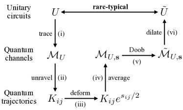
Figure 2: Post-selecting rare trajectories of one circuit as typical trajectories of another. Tracing over a brickwork circuit (i) generates a Markovian channel $\mathcal{M}$. which is unravelled (ii) to yield Kraus operators $\{K\}$ and quantum trajectories. Post-selection is achieved by reweighting the trajectories (iii) or equivalently by tilting the channel with a biasing field $s$ (iv). The quantum Doob transformation (v) yields a new channel $\tilde{\mathcal{M}}_{\boldsymbol{s}}$ which optimally generates the post-selected (rare) trajectories. Finally, a dilation of this channel (vi) provides a new brickwork circuit with gate $\tilde{U}$.

Setup. Consider a one-dimensional unitary brickwork quantum circuit, i.e., a chain of $2L$ qubits evolved in time by the staggered application of two-qubit unitary gates. The system state at time $t\in\mathbb{N}$ is $\ket{\Psi_{t}}=\mathbb{U}^{t}\ket{\Psi_{0}}$ where $\ket{\Psi_{0}}$ is the initial state and

$$\mathbb{U}=\bigotimes_{x=1}^{L}U_{x-1/2,x}\bigotimes_{x=1}^{L}U_{x,x+1/2}\,.$$ (1)

We label sites by half integers, use periodic boundary conditions, and denote by $U_{x,y}$ the operator acting as the two-qubit gate $U\in{\rm U}(4)$ on the qubits at positions $x$ and $y$ (and the identity elsewhere). Fig. 1(a) shows the circuit in the standard diagrammatic representation of tensor networks (TNs) [37].

We now implement the following measurement scheme: every half time step $\tau\in[0,t]\cap\mathbb{Z}/2$ we measure in the computational basis $\{\ket{0},\ket{1}\}$ the qubits at spatial positions $\tau\pm 1/2$ (i.e., along the direction of the light-cone), see Fig. 1(b). These measurements make the evolution stochastic. Denoting by $\ket{\Psi_{\tau}}$ the state of the system at $\tau$, the probability of measuring at time $\tau+1/2$ the qubit at position $\tau$ in the state $\ket{i}$ and that at position $\tau+1$ in the state $\ket{j}$ is given by $\|\mathbb{K}_{ij}(\tau)\ket{\Psi_{\tau}}\|^{2}$, where the many-body Kraus operators are

$$\!\!\!\!\mathbb{K}_{ij}(\tau)\!=\!\begin{cases}\displaystyle P^{(i)}_{\tau}P^{(j)}_{\tau+1}\bigotimes_{x=1}^{L}U_{x-1/2,x}&\tau\in\mathbb{Z}+{1}/{2}\\ \\ \displaystyle P^{(i)}_{\tau}P^{(j)}_{\tau+1}\bigotimes_{x=1}^{L}U_{x,x+1/2}&\tau\in\mathbb{Z}\end{cases}\!\!,$$ (2)

and $P^{(i)}$ denotes a projector on the state $\ket{i}$ of the computational basis. The (normalised) state of the system after the measurement is then $\mathbb{K}_{ij}(\tau)\ket{\Psi_{\tau}}/\|\mathbb{K}_{ij}\ket{\Psi_{\tau}}\|$. A full measurement sequence generates the quantum trajectory $(\boldsymbol{i},\boldsymbol{j})=(i_{0},\ldots,i_{2t},j_{0},\ldots,j_{2t})$ occurring with probability $\|\mathbb{K}_{\boldsymbol{i}\boldsymbol{j}}(t)\ket{\Psi_{0}}\|^{2}$, where $\mathbb{K}_{\boldsymbol{i}\boldsymbol{j}}(t)\equiv\mathbb{K}_{i_{2t}j_{2t}}(t-1/2)\cdots\mathbb{K}_{i_{0}j_{0}}(-1/2)$ .

Consider now the infinite temperature correlation function for one qubit along the light-cone passing through $x=0$. For a given trajectory this reads

$$\!\!C^{ab}_{(\boldsymbol{i},\boldsymbol{j})}(t)\!=\frac{1}{2^{2L}}\sum_{\boldsymbol{s}}\expectationvalue{\mathbb{K}_{\boldsymbol{i}\boldsymbol{j}}^{{\dagger}}(t)a_{t}\mathbb{K}^{\phantom{{\dagger}}}_{\boldsymbol{i}\boldsymbol{j}}(t)b_{0}}{\boldsymbol{s}},$$ (3)

where $\{\ket{\boldsymbol{s}}\}$ is a basis of the Hilbert space and we used the notation $a_{x}$ to denote the operator that acts non-trivially, as $a\in{\rm End}(\mathbb{C}^{2})$, only at site $x$. In graphical form Eq. (3) is given in Fig. 1(c). This TN can be drastically simplified because the causal light-cones of the two operators overlap only on one line in the discrete space time (cf. Refs. [22, 39, 40, 41]). For $L>2t+1$ this yields Fig. 1(d), or in formulae,

$$\!\!C^{ab}_{(\boldsymbol{i},\boldsymbol{j})}(t)\!=\!\tr[aK^{\phantom{{\dagger}}}_{i_{2t}j_{2t-1}}\!\!\cdots K^{\phantom{{\dagger}}}_{i_{1}j_{0}}bK^{\dagger}_{i_{1}j_{0}}\!\!\cdots K^{\dagger}_{i_{2t}j_{2t-1}}],$$ (4)

where the single site Kraus operators are

$$\matrixelement{m}{K_{ij}}{n}=\frac{1}{\sqrt{2}}\matrixelement{im}{U}{nj}\,.$$ (5)

Summing over all trajectories, we recover the dynamical correlator along the light-cone of the unmeasured circuit,

$$\sum_{\boldsymbol{i},\boldsymbol{j}}C^{ab}_{(\boldsymbol{i},\boldsymbol{j})}(t)=C^{ab}(t)=\tr[a\mathcal{M}^{2t}_{U}[b]],$$ (6)

where

$$\mathcal{M}_{U}[\rho]=\frac{1}{2}\tr_{A}[U(\rho\otimes\mathbf{1}_{B})U^{\dagger}],$$ (7)

is the quantum channel for the average dynamics of a single qubit along the light-cone (cf. Refs. [22, 39, 40, 41]), with $\tr_{A}[\cdot]$ the trace over the first site. Equation (6) holds because the channel is “unravelled” [42] by the $\{K_{ij}\}$

$$\mathcal{M}_{U}[\cdot]=\sum_{i,j}K_{ij}\cdot K^{\dagger}_{ij}.$$ (8)

Reweighting of trajectories and large deviations. We aim to characterise correlations along quantum trajectories in a way that sidesteps the post-selection problem. We follow the protocol of Fig. 2, in which steps (i) and (ii) correspond to the derivation of $\mathcal{M}_{U}$ and $K_{ij}$ above. We now execute steps (iii) to (v) (see [44] for details).

Instead of focusing on a specific trajectory, we consider a “soft” post-selection of all trajectories characterised by a certain pattern of measurement outcomes in the limit of large time $t$. This is amenable to quantum large deviation methods (LD) [45, 46]. Starting from the sum over measurement outcomes in Eq. (6), we (exponentially) reweight some terms with respect to others. The resulting biased ensemble of trajectories is encoded in a deformed (or “tilted”) quantum channel ${\mathcal{M}}_{U,s}$ [46].

Consider the trajectory determined by the sequence $((i_{0},j_{1}),\ldots,(i_{2t-1},j_{2t}))$, where $(i_{k},j_{k+1})$ denotes a binary pair of outcomes for $k=1,\ldots,2t-1$ (cf. the configuration of a classical Ising model on a ladder, where $k$ denotes a rung). We reweight the trajectories based on how many rungs have outcome pairs $(0,0)$, $(1,0)$, $(0,1)$, and $(1,1)$. This is achieved by introducing four counting fields $\boldsymbol{s}=\{s_{ij}\}_{i,j=0,1}$ and modifying the sum in Eq. (6),

$$\sum_{\boldsymbol{i},\boldsymbol{j}}e^{-\sum_{l,m}s_{lm}Q_{lm}(\boldsymbol{i},\boldsymbol{j})}C^{ab}_{(\boldsymbol{i},\boldsymbol{j})}(t,t)\equiv\tr[a\mathcal{M}^{2t}_{U,\mathbb{s}}[b]]$$ (9)

where $Q_{lm}(\boldsymbol{i},\boldsymbol{j})=\sum_{k=1}^{2t}\delta_{i_{k-1},l}\delta_{j_{k},m}$. Since the sums on each rung are independent the tilted channel reads [46]

$$\mathcal{M}_{U,\mathbb{s}}[\rho]=\sum_{i,j}e^{-{s}_{ij}}K_{ij}\rho K^{\dagger}_{ij}.$$ (10)

This result implements steps (iii) and (iv) of Fig. 2.

Note that since the sum of all $Q_{\mu\nu}(\boldsymbol{i},\boldsymbol{j})$ is fixed to $2t-1$, the bias $\boldsymbol{s}$ corresponds to three non-trivial fields. The exponential tilting in Eq. (10) controls the average number of outcomes of each type, instead of their exact values, but these “soft-constrained” (canonical) trajectory ensembles are equivalent to “hard-constrained” (microcanonical) ensembles, for large times [47].

The operator $\mathcal{M}_{U,\mathbb{s}}$ is not trace-preserving [its leading eigenvalue $e^{\theta(\mathbb{s})}\neq 1$ in general], so it is not a physical quantum map. Step (v) of Fig. 2 performs the quantum version [46, 48, 49, 50] of a generalised Doob transform [51, 52], yielding a new trace-preserving channel which reproduces the biased trajectory ensemble. Specifically,

$$\tilde{\mathcal{M}}_{U,\mathbb{s}}[\cdot]=\sum_{i}\tilde{K}_{i}\cdot\tilde{K}_{i}^{\dagger},\;\;\;\tilde{K_{i}}=\frac{e^{-s_{i}/2}}{e^{\theta(\mathbb{s})/2}}l^{1/2}_{\mathbb{s}}K_{i}l^{-1/2}_{\mathbb{s}},$$ (11)

with $l_{\mathbb{s}}$ the leading left eigenmatrix of $\mathcal{M}_{U,\mathbb{s}}$. In terms of $\tilde{\mathcal{M}}_{U,\mathbb{s}}$, the reweighted trajectories (9) are

$$\!\!\!\!\tr[a\mathcal{M}^{2t}_{U,\mathbb{s}}[b]]\!\!=\!e^{2t\theta(\mathbb{s})}\!\tr[l^{-1/2}_{\mathbb{s}}al^{-1/2}_{\mathbb{s}}\tilde{\mathcal{M}}^{2t}_{U,\mathbb{s}}[l^{1/2}_{\mathbb{s}}bl^{1/2}_{\mathbb{s}}]]\!.$$ (12)

Hence, typical trajectories of the channel (11) reproduce the rare trajectories of the original $\mathcal{M}_{U}$, as encoded in the tilted $\mathcal{M}_{U,\mathbb{s}}$.

Unitary circuit realising the rare events. We now turn to step (vi) in Fig. 2, which is motivated by the question:

• Can one find an $\mathbb{s}$-dependent unitary operator $\tilde{U}\in{\rm End}(\mathbb{C}^{2}\otimes\mathbb{C}^{2})$ such that $\tilde{\mathcal{M}}_{U,\mathbb{s}}$ is given by Eq. (7) with $U$ replaced by $\tilde{U}$?

We present cases where the answer is affirmative, meaning that a brickwork circuit with gate $\tilde{U}$ has typical light-cone trajectories that replicate rare post-selected trajectories of $U$.

One might expect that $\tilde{U}$ can always be found, because Eq. (7) is an environmental representation $\mathcal{M}_{\tilde{U}}$ [42]. The Stinespring dilation theorem [53] guarantees existence of some environmental representation, but our question is more restrictive because (a) both system and environment in Eq. (7) must be isomorphic to $\mathbb{C}^{2}$ (i.e., the dilation defines a unitary circuit similar to the original one); (b) the environment has to be in the maximally mixed state (i.e., we seek a unistochastic channel [42]). In fact, Eq. (7) already implies that $\mathcal{M}_{\tilde{U}}$ is unital [$\mathcal{M}_{\tilde{U}}(\mathbf{1})=\mathbf{1}$], so existence of $\tilde{U}$ requires that $\tilde{\mathcal{M}}_{U,\mathbb{s}}$ is also unital, which is not the case in general. Hence, while steps (i-v) in Fig. 2 can be performed for any $U$ and $\mathbb{s}$, step (vi) is restricted to specific cases of the post-selection problem.

To illustrate this, we focus on circuits where $U$ is an XYZ gate: $U=U_{\rm{XYZ}}(\{J_{i}\})$, with

$$U_{\rm{XYZ}}(\{J_{i}\})=e^{-i({J_{x}}\sigma_{x}\otimes\sigma_{x}+{J_{y}}\sigma_{y}\otimes\sigma_{y}+{J_{z}}\sigma_{z}\otimes\sigma_{z})/2}\!,$$ (13)

where $\{\sigma_{i}\}_{i=x,y,z}$ are Pauli matrices and $(J_{x},J_{y},J_{z})\in[-\pi,\pi]$. This implies a $\mathbb{Z}_{2}$ symmetry $\tilde{\mathcal{M}}_{U,\mathbb{s}}[\sigma_{z}(\cdot)\sigma_{z}]=\sigma_{z}\tilde{\mathcal{M}}_{U,\mathbb{s}}(\cdot)\sigma_{z}$ for all $\mathbb{s}$, which relies on the fact that $\sigma_{z}$ is diagonal in the measurement basis of Eq. (2). To replicate this, we also seek $\tilde{U}$ in XYZ form with $\mathbb{s}$-dependent couplings $\{J^{\prime}_{\mathbb{s},i}\}_{i=x,y,z}$. This choice of $\tilde{U}$ implies the additional symmetry ${\mathcal{M}}_{\tilde{U}}[\sigma_{x}(\cdot)\sigma_{x}]=\sigma_{x}{\mathcal{M}}_{\tilde{U}}(\cdot)\sigma_{x}$.

Writing explicitly the dependence of the channels on the couplings, finding $\tilde{U}$ amounts to solving

$$\tilde{\mathcal{M}}_{U,\boldsymbol{s}}(\{J_{i}\})={\mathcal{M}}_{\tilde{U}}(\{J^{\prime}_{\mathbb{s},i}\})\,,$$ (14)

for real couplings $\{J^{\prime}_{\mathbb{s},i}\}$. The symmetries of ${\mathcal{M}}_{\tilde{U}}$ restrict solutions to cases where $\tilde{\mathcal{M}}_{\boldsymbol{s}}$ is both unital and $\mathbb{Z}_{2}$-symmetric. These are the post-selection problems that may be solved by constructing $\tilde{U}$. Explicit computation of $\tilde{\mathcal{M}}_{U,\mathbb{s}}$ is given in [44], revealing several classes of solution for $\tilde{U}$.

The first class is when any two of the $J_{i}$ are equal to $\pm\pi/2$, making $U$ dual unitary [22, 23]. For example

$$U_{\rm{XYZ}}(\{\tfrac{\pi}{2},\tfrac{\pi}{2},J_{j}\})=Se^{-i(J_{j}-\pi/2)(\sigma_{j}\otimes\sigma_{j})/2},$$ (15)

where $J_{j}$ is the coupling not equal to $\pi/2$ and $S$ is the SWAP gate. In these cases a dual-unitary $\tilde{U}$ also exists of the form (15). These post-selection problems are simple because $K_{ij}K^{\dagger}_{ij}=c_{ij}\mathbf{1}$ for all $i,j$ (with $c_{ij}\geq 0$). This means that the channel $\mathcal{M}$ is a classical mixture of unitary channels, a measurement $(i_{k-1},j_{k})$ in $C_{(\boldsymbol{i},\boldsymbol{j})}$ occurs with probability $c_{i_{k-1},j_{k}}$ independent of other measurements, and the count statistics is multinomial. This simplicity is evident in the fact that $l_{\boldsymbol{s}}=\mathbf{1}$, making the Doob transform (11) straightforward, with $\tilde{\mathcal{M}}_{U,\boldsymbol{s}}$ a different mixture of the same unitaries as in $\mathcal{M}$. This result establishes an interesting connection to random unitary circuits [9]: atypical measurement outcomes in (space-time) translation invariant dual unitary circuits are equivalent to the evolution under atypical sequences of i.i.d. random unitaries along the light-cone.

The other classes of solution to Eq. (14) restrict the counting fields to $s_{00}=s_{11}$, ensuring that $\tilde{M}_{\boldsymbol{s}}$ is unital [44]. This means that $(0,0)$ measurement pairs cannot be selected preferentially over $(1,1)$. The $\mathbb{Z}_{2}$ symmetry requires either (A) $s_{01}=s_{10}$; or (B) $\sin J_{x}=\sin J_{y}$; or (C) $J_{z}=\pm\pi/2$. Post-selection is simple in case (A) because the counting fields only differentiate the outcomes with $i_{k-1}=j_{k}$ from those with $i_{k-1}\neq j_{k}$; these two possibilities are again independent for all $k$, with $l_{\boldsymbol{s}}=\mathbf{1}$. In case (B) one has ${K_{01}\propto K_{10}^{\dagger}\propto\sigma^{\pm}}\equiv(\sigma_{x}\pm i\sigma_{y})/2$ while $K_{00},K_{11}$ both commute with $\sigma_{z}$. Here $l_{\boldsymbol{s}}\neq\mathbf{1}$ and measurements at different times are not independent, but the post-selected trajectories simplify in a different way: for sufficiently large times the conditional state $K^{\phantom{{\dagger}}}_{i_{2t}j_{2t-1}}\!\!\cdots K^{\phantom{{\dagger}}}_{i_{1}j_{0}}|\psi\rangle$ must be an eigenstate of $\sigma^{z}$ and the system behaves classically. Transitions between the two eigenstates are signalled by $(1,0)$ and $(0,1)$ measurement pairs, which appear in an alternating sequence, interspersed by random $(0,0)$s and $(1,1)$s.

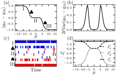
Figure 3: Illustration of the subcase (C) for circuit parameters $J_{x}=0.205\pi$ and $J_{y}=0.2\pi$, and tilting parameters $s_{00}=s_{11}=0$ and $s_{01}=-s_{10}$. (a,b) Mean and (normalised) variance of the accumulated number of $(0,1)$ minus $(1,0)$ measurements. (c) Typical trajectories for $\mu=0,\pm 10$ [regimes (I,II,III)] and $\mu=\pm 5.282$ [crossover points where $\text{Var}(q_{01}-q_{10})$ is maximised, marked by $(\clubsuit,\spadesuit)$]. Measurement outcomes $(1,0)$ and $(0,1)$ are marked in blue and red; $(0,0)$ and $(1,1)$ are not shown. (d) The new circuit parameters $\{J^{\prime}_{i}\}$ that realise the Doob transformation of the original circuit.

The final case (C) is not simple and exhibits an interesting dynamical crossover under post-selection. We assume $J_{x}>J_{y}$ and $J_{z}=+\pi/2$ for concreteness. Defining $\mu\equiv(s_{01}-s_{10})/2$ and $\delta=\sin[(J_{x}-J_{y})/2]/\cos[(J_{x}+J_{y})/2]$, one finds

$$\tilde{K}_{10} =A(\mu,\delta)\begin{pmatrix}0&\sqrt{\delta^{2}+e^{2\mu}}\\ -\delta\sqrt{1+\delta^{2}e^{2\mu}}&0\end{pmatrix},$$ (16)

$$\tilde{K}_{01} =A(\mu,\delta)\begin{pmatrix}0&-\delta e^{\mu}\sqrt{\delta^{2}+e^{2\mu}}\\ e^{\mu}\sqrt{1+\delta^{2}e^{2\mu}}&0\end{pmatrix},$$

while $\tilde{K}_{00}$ and $\tilde{K}_{11}$ only depend on $\mu$ through a multiplicative constant (see [44] for details). For $\delta\ll 1$ we have the following three regimes:

$${\rm(I)} \!\!\!\tilde{K}_{10}\propto\sigma_{y},\quad\tilde{K}_{01}\propto\delta^{-1}e^{\mu}\sigma_{-},\quad e^{\mu}\ll\delta\,,$$ (17)

$${\rm(II)} \!\!\!\tilde{K}_{10}\propto\sigma_{+},\quad\tilde{K}_{01}\propto\sigma_{-},\quad\delta\!\ll\!e^{\mu}\!\ll\!{\delta^{-1}},$$ (18)

$${\rm(III)} \!\!\!\tilde{K}_{10}\propto\delta^{-1}e^{-\mu}\sigma_{+},\quad\tilde{K}_{01}\propto\sigma_{y},\quad e^{\mu}\gg{\delta^{-1}}\,,$$ (19)

as shown in Figure 3. Regime (II) includes typical trajectories ($\mu\approx 0$): it resembles case (B) in that (1,0) and (0,1) alternate, interspersed with (0,0)s and (1,1)s. In contrast, regimes (I,III) describe trajectories that are post-selected for an overwhelming majority of either (1,0) or (0,1) measurements, breaking the alternating structure. All three regimes have highly-structured measurement records (either alternating or dominated by one outcome) and are separated by crossovers where the records have much larger variance, Fig. 3(b,c).

The behaviour in the three regimes can be reproduced by a suitable $\tilde{U}$ gate, whose couplings are plotted in Fig. 3(d). From Eq. (7) the eigenvalues of the channel are given in terms of the couplings by $(1,\sin{J_{x}^{\prime}}\sin{J_{y}^{\prime}},\sin{J_{x}^{\prime}}\sin{J_{z}^{\prime}},\sin{J_{y}^{\prime}}\sin{J_{z}}^{\prime})$ [44], meaning that the spectral gap of the Doob channel does not close during the crossovers. Instead, $\tilde{U}$ crosses over from $\tilde{U}\simeq U$ in regime (II) to an almost dual-unitary gate in regimes (I,III). The sharpness of this crossover reflects the rigid alternating structure of typical trajectories, so that large counting fields $|\mu|\sim\log(1/\delta)$ are required to post-select any other outcomes.

Conclusions. We studied the interplay between unitary dynamics and rare measurements outcomes in quantum circuits. We showed that a class of post-selection problems, specifically that of biasing dynamics according to the large deviations in the number of measurement outcomes along the light-cone, can be resolved by mapping to a different circuit for which the rare events are the (easy to access) typical behaviour. This provides an efficient way to access properties of quantum trajectories in real experiments avoiding post-selection overheads.

Even though our results are obtained in a heavily simplified setting, they are in our view an important proof of principle: it is sometimes possible to embed the effect of measurements in a quantum many-body system by studying the purely unitary dynamics of a different system. There are many interesting follow-up questions. Cases where $U\neq U_{\rm{XYZ}}$ are briefly discussed in [44]. One may also extend the general method here to finite times, instead of $t\to\infty$. Another important extension would be to study more complicated trajectory re-weightings, in particular those relevant to studying measurement-induced entanglement phase transitions. Finally, here we insisted on the new quantum circuit being unitary. One can however relax this constraint and seek for a hybrid circuit with unitary evolution and forced measurements, for example by admitting $\{J^{\prime}_{\mathbb{s},i}\}\in\mathbb{C}$ in Eq. (14). This more general mapping also resolves the post selection problem.