On the good reliability of an interval-based metric to validate prediction uncertainty for machine learning regression tasks

Abstract

This short study presents an opportunistic approach to a (more) reliable validation method for prediction uncertainty average calibration. Considering that variance-based calibration metrics (ZMS, NLL, RCE…) are quite sensitive to the presence of heavy tails in the uncertainty and error distributions, a shift is proposed to an interval-based metric, the Prediction Interval Coverage Probability (PICP). It is shown on a large ensemble of molecular properties datasets that (1) sets of z-scores are well represented by Student’s-$t(\nu)$ distributions, $\nu$ being the number of degrees of freedom; (2) accurate estimation of 95 % prediction intervals can be obtained by the simple $2\sigma$ rule for $\nu>3$; and (3) the resulting PICPs are more quickly and reliably tested than variance-based calibration metrics. Overall, this method enables to test 20 % more datasets than ZMS testing. Conditional calibration is also assessed using the PICP approach.


Note: the present study is essentially an addendum to Ref.(Pernot2024, ), and the reader is invited to consult this reference for details on the notations and concepts.

I Introduction

A recent study(Pernot2024, ) showed that the reliability of average calibration statistics for prediction uncertainties and of their validation is strongly affected by the shape of the uncertainties ($u_{E}$) and error ($E$) distributions, and notably by the presence of heavy tails or outliers. If one considers the ZMS statistic, the mean squares value of z-scores $Z=E/u_{E}$, it was shown that datasets with $\beta_{GM}(Z^{2})\geq 0.8$ cannot be reliably tested for calibration using the $ZMS=1$ test, where $\beta_{GM}(.)$ is a robust skewness metric(Groeneveld1984, ; Bonato2011, ; Pernot2021, ). For a recently published database of 33 datasets of ML materials properties(Jacobs2024, ), this means that only about half of them could reliably be tested for ZMS calibration. Things are even worse for the RCE statistic [$RCE=\left(\sqrt{<u_{E}^{2}>}-\sqrt{<E^{2}>}\right)/\sqrt{<u_{E}^{2}>}$] , which is sensitive to both $u_{E}$ and $E$ distributions. This limits considerably the applicability of variance-based calibration statistics.

The present proposition draws on three points that will be detailed below:

• the distributions of $Z$ values are very close to scaled Student’s-t, noted $t_{s}(\nu)$;

• the $t_{s}(\nu)$-based enlargement factor $k_{95}$ to convert the standard deviation of $Z$ to the half-range of a 95 % probability interval does not vary strongly with the $\nu$ parameter for $\nu>3$;

• for large datasets, testing a prediction interval by its coverage probability is more reliable and less costly than testing a ZMS value, which requires bootstrapping(Pernot2024, ).

These observations enable to define a simpler alternative approach to average calibration validation. Sect. II develops and justifies the three central points of the approach. PICP testing is then applied to Jacobs et al.’s datasets and compared with ZMS testing (Sect. III), and extended to conditional calibration. A brief conclusion is provided next.

II Interval-based average calibration testing

II.1 PICP and its validation

In practice, the PICPs are estimated as frequencies over a validation set(Pernot2022b, )

$$PICP_{p}=\frac{1}{M}\sum_{i=1}^{M}\boldsymbol{1}\left(|Z|\leq k_{p}\right)$$ (1)

where $p$ is a percentage value, $\boldsymbol{1}(x)$ is the indicator function for proposition $x$, taking values 1 when $x$ is true and 0 when $x$ is false. Confidence intervals $[PICP_{p}^{-},PICP_{p}^{+}]$ on PICP values are derived from properties of the binomial distribution(Pernot2022b, ). The continuity-corrected Wilson method(Newcombe1998, ) is used here, following the recommendation of Pernot(Pernot2022a, ), Sect. D.1. Note that the datasets studied here are large enough to avoid the potential problems described in this study.

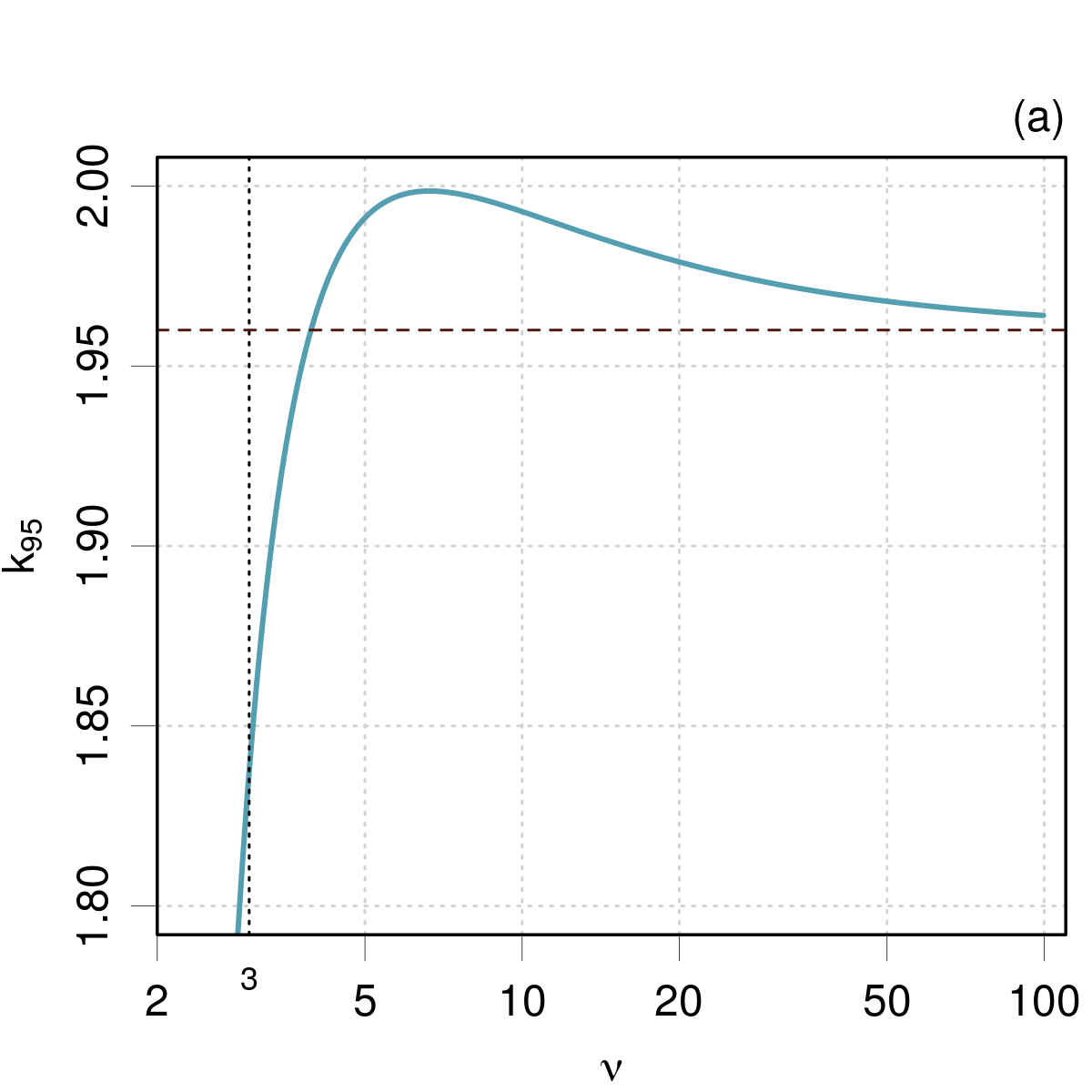
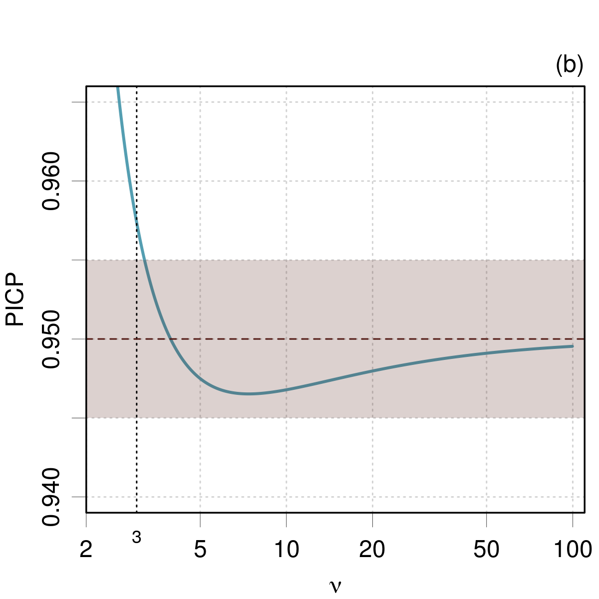
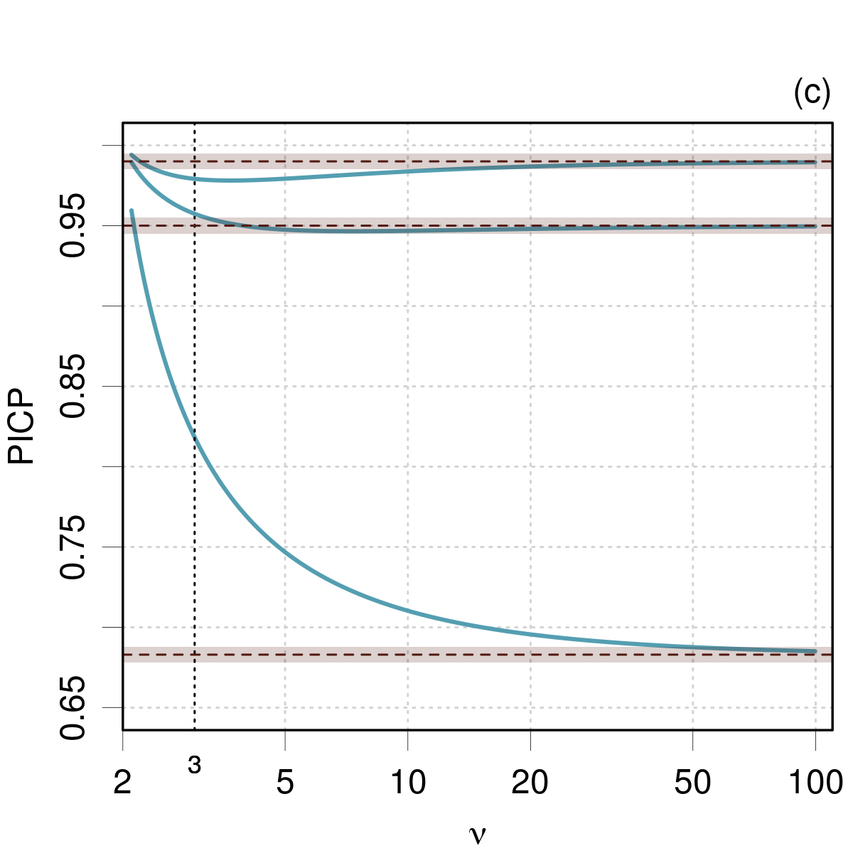
Figure 1: Enlargement factor and coverage probabilities for a $t_{s}(\nu)$ distribution as a function of $\nu$: (a) $k_{95}$ ; (b) coverage probability of a $[-a,a]$ interval for (b) $a=1.96$; (c) $a=1,\,1.96,\,2.83$. The grayed area depicts a 0.005 deviation around the asymptotic value.

Formally, testing a PICP value for a $p$ % prediction interval is based on checking that the target probability belongs to the PICP confidence interval, i.e.

$$p/100\in[PICP_{p}^{-},PICP_{p}^{+}]$$ (2)

II.2 Coverage of $2\sigma$ intervals for $t_{s}(\nu)$ as a function of $\nu$

The enlargement factor $k_{95}$ to convert $u_{E}$ to $U_{95}=k_{95}u_{E}$ (the half range of a 95 % confidence/prediction interval) for unit-variance $t_{s}(\nu)$ stays very close to the normal asymptotic value (1.96) for $\nu\geq 3$. One can see on Fig. 1(a) that it is non-monotonous with $\nu$ and varies between 1.85 and 2, with a maximum at about $\nu=6.7$. The $k_{95}=1.9$ value is reached at $\nu\simeq 3.3$. In such conditions, using $k_{95}=1.96$ instead of the exact value represents at most a 6 % error on the enlargement factor. Using a fixed enlargement factor is important, as it avoids altogether to fit the $Z$ sample by a $t_{s}(\nu)$ distribution.

Let us consider the reverse problem, i.e. how the expected coverage probability varies with $\nu$ when using a fixed value $k_{95}=1.96$. One sees on Fig. 1(b) that the deviation from the 0.95 target is at most 0.005 for $\nu>3$, which is very small when compared to the uncertainty on empirical PICP values expected for moderately sized samples(Pernot2022a, ). Note that this observation is not generalizable to other intervals, such as $1\sigma$ or $3\sigma$ , as can be seen on Fig. 1(c), where the PICP values deviate more strongly from their target than in the $2\sigma$ case (in all rigor, one should write $1.96\sigma)$.

In order to relax slightly the validation criterion to conform with a maximal deviation from the theoretical value of 0.005, the following test is used in practice instead of Eq. 2

$$0.945\leq PICP_{95}^{+}\,\&\,PICP_{95}^{-}\leq 0.955$$ (3)

II.3 Simulations

PICP₉₅ has been estimated for a series of $Z$ samples generated from $t_{s}(\nu)$ distributions with degrees of freedom varying between 2 and 100. The samples contain $M=10000$ points. The results are reported in Fig. 2(left). One sees that invalid intervals are essentially obtained for $\nu\leq 3$, in agreement with Sect. II.2. When converted to $Z^{2}$ skewness, this corresponds to $\beta_{GM}(Z^{2})\geq 0.85$ [Fig. 2(left)]. These thresholds expand significantly the reliability range for testing when compared to the ZMS values ($\nu\geq 6$ or $\beta_{GM}(Z^{2})\leq 0.8$)(Pernot2024, ).

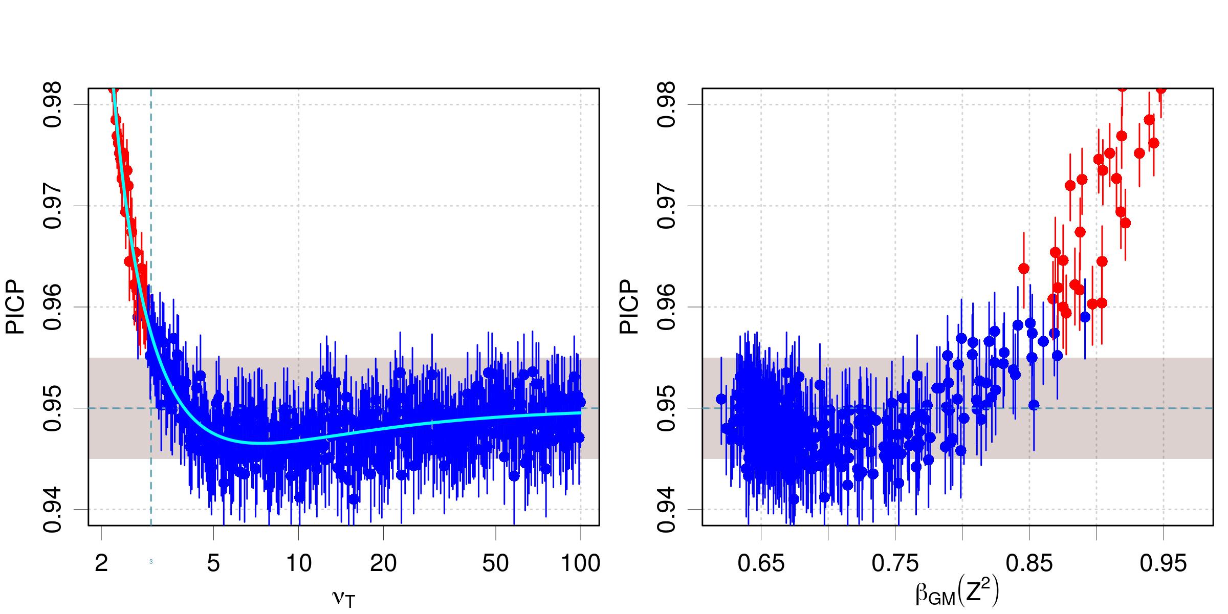
Figure 2: PICP₉₅ values for $t(\nu)$ samples: (left) effective coverage as a function of $\nu$; (right) same data as a function of the $Z^{2}$ skewness. The 95% confidence intervals on the PICP values are displayed as error bars. The cyan curve is the theoretical curve, as seen in Fig. 1(b). The gray area depicts the validity interval. The red points depict invalidated intervals that do not overlap the gray area.

Note that for ZMS, the threshold for $\beta_{GM}(Z^{2})$ was estimated from the loss of reliability in the estimation of confidence intervals by bootstrapping(Pernot2024, ), while for PICP, it is based on an error limit for using a fixed enlargement factor ($k_{95}=1.96$).

III Application

Jacobs et al.(Jacobs2024, ) published an ensemble of 33 datasets of ML materials properties, with predictions by random forest models. The prediction uncertainties in these datasets have been calibrated pos-hoc, by polynomial transformation.

After checking the Student’s distribution hypothesis for z-scores, the PICP analysis is performed and compared to the results for ZMS reported in the Appendix of Ref.(Pernot2024, ).

III.1 Shape of $Z$ distributions

Assuming that $Z$ has a unit-variance Student’s-$t$ distribution with $\nu$ degrees of freedom ($Z\sim t_{s}(\nu)$), $Z^{2}$ has a unit-variance Fisher-Snedecor distribution(Evans2000, ) with degrees of freedom $1$ and $\nu$ ($Z^{2}\sim F_{s}(1,\nu)$)(Pernot2024, ). To assess this distribution hypothesis, the $Z^{2}$ datasets have been fitted by a scaled $F$ distribution, and the results are reported in the Appendix A (Figs. 7-12). The fits are done by maximum goodness-of-fit estimation using the Kolmogorov-Smirnov distance (Delignette2015, ). For each dataset, the quality of the fit is estimated by visual comparison of the histogram of $Z^{2}$ values with the best fit density function.

Indeed, the fits are very good for all sets, except for Set 1 and 13, which are furthermore not testable (see below). Note that Sets 1 and 13 have also been pointed out(Pernot2024, ) for having a large fraction of null z-scores, which is likely to affect the fitting. The shape parameters (reported in the title of each plot) cover a wide range, from 1 to 1743, with a number of very small values (below 6)(Pernot2024, ) revealing heavy tails. Large values indicate quasi-normal $Z$ distribution.

It has to be noted that the best-fit values of the shape parameter $\nu$ might be sensitive to the choice of fitting method and to the adequacy of the chosen distribution. The present values are only indicative and a complex uncertainty analysis involving model inadequacy, parametric and statistical uncertainties would be necessary to derive reliable estimates(Pernot2017, ). This is why $\nu$ is not used in practice as a threshold for the selection of testable datasets. Nevertheless, the overall quality of the fits confirms the pertinence of the Student’s distribution hypothesis for the studied z-scores.

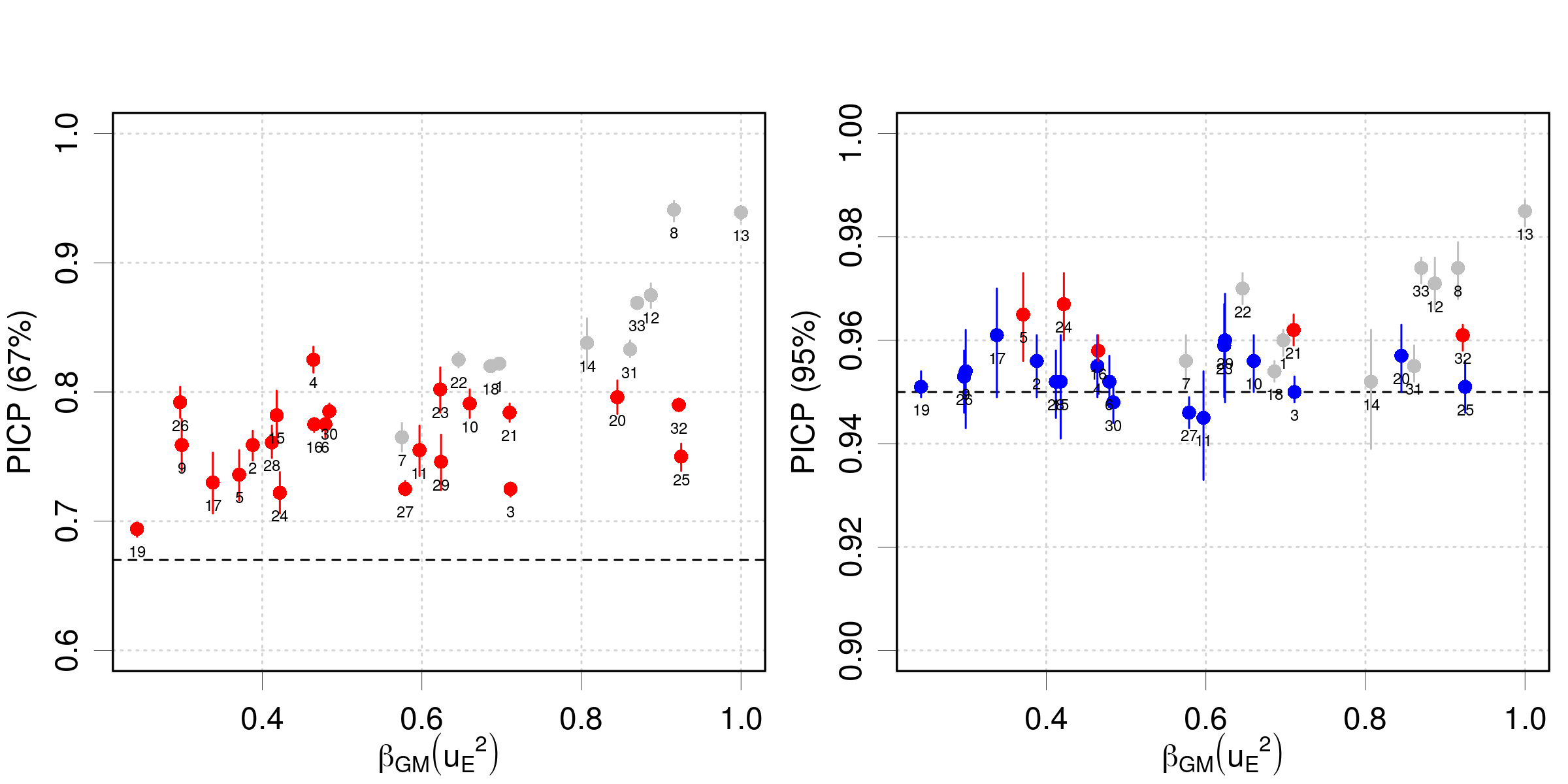
Figure 3: PICP analysis at the $1\sigma$ (left) and $2\sigma$ (right) levels. The 95% confidence intervals on the PICP values are displayed as error bars. The points are color-coded into three classes: (1) gray for sets with $\beta_{GM}(Z^{2})\geq 0.85$; (2) blue for calibrated sets; and (red) for uncalibrated sets.

III.2 Untestable datasets

It was stated in Sect. II.3 that datasets with $\beta_{GM}(Z^{2})\geq 0.85$ cannot be reliably tested by the proposed PICP metric. This concerns 10 sets: 1, 7, 8, 12, 13, 14, 18, 22, 31 and 33, a subset of the 16 sets with $\beta_{GM}(Z^{2})\geq 0.80$ that would be unsuitable for testing by their ZMS value. Using PICP enables thus to test about 20 % more sets than ZMS.

III.3 PICP analysis

The PICP at the $1\sigma$ and $2\sigma$ levels for the 33 datasets are reported in Fig. 3, where the points are sorted according to the skewness of the squared uncertainties distribution. One sees that none of the PICP₆₇ values are compatible with the 67 % target. The values are all overestimated, with a positive trend according to $\beta_{GM}(u_{E}^{2})$. The untestable sets occur for $\beta_{GM}(u_{E}^{2})\geq 0.6$.

At the PICP₉₅ level, a large portion of the testable sets (18/23) is validated. It is remarkable that the rejected sets (5, 16, 21, 24 and 32) have PICP values in slight excess only, not exceeding 0.97.

A contingency table is used for the comparison with the results of ZMS validation (Table 1), based on the classification of the datasets into three classes (valid, invalid and untestable). If one considers the 17 datasets for which the validity comparison can be made (16 are excluded by ZMS), the PICP and ZMS metrics agree for 13 of them, but conflict for 4 (Sets 6, 16, 28 and 32). From the 6 datasets that were deemed untestable by ZMS and testable by PICP, 5 are validated. So globally, PICP validates 18 sets and invalidates 5, where ZMS validated 13 and invalidated 4.

		ZMS
		valid	invalid	untestable	Sum
	valid	11	2	5	18
PICP	invalid	2	2	1	5
	untestable	0	0	10	10
	Sum	13	4	16	33

Table 1: Contingency table for the validation by ZMS (rows) and PICP (columns) metrics.

III.4 LCP analysis

A local version of the PICP analysis, the LCP analysis(Pernot2022b, ), can be applied to the 18 datasets with validated PICP values to assess their consistency(Pernot2023d, ), using 20 equal-size $u_{E}$-based bins (Figs. 4-6). As the post-hoc calibration used to design those datasets is based on a polynomial correction of the uncertainties intended to correct for major unsuitable trends in uncertainty space, on should expect a reasonable consistency for most datasets.

The number of untestable bins per set is very small, varying from 0 to a maximum of 5 for Set 26. Similarly, very few bins are invalidated, the most problematic case being Set 30 with 4 rejected bins. For this set, uncertainty values between 0.2 and 0.3 seem to be consistently underestimated. For Set 23, there seems to be a residual trend from under- to over-estimation of $u_{E}$. Similar features are visible for Sets 27 and 28, while Set 26 seems to suffer from a notable underestimation of large uncertainties.

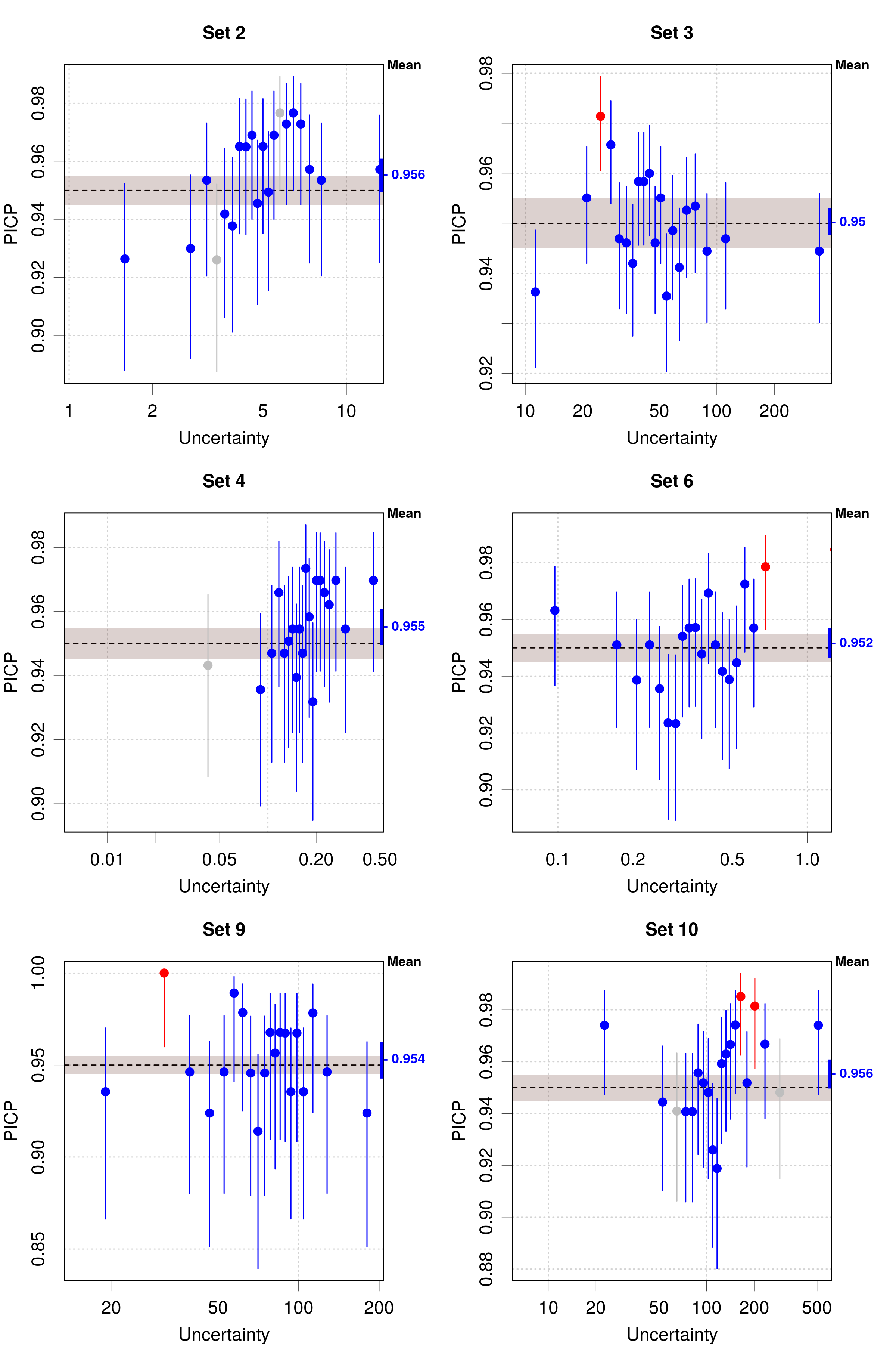
Figure 4: Local PICP (LCP) analysis using $N=20$ uncertainty-based equal-size bins. The 95 % confidence intervals on the local PICP values are reported as error bars. The average PICP value is reported in the right margin. The gray area represents an admissible 0.005 deviation around the target value. Local values incompatible with this admissible area are colored in red. Gray points cannot be reliably tested.

Figure 5: Fig. 4, continued.

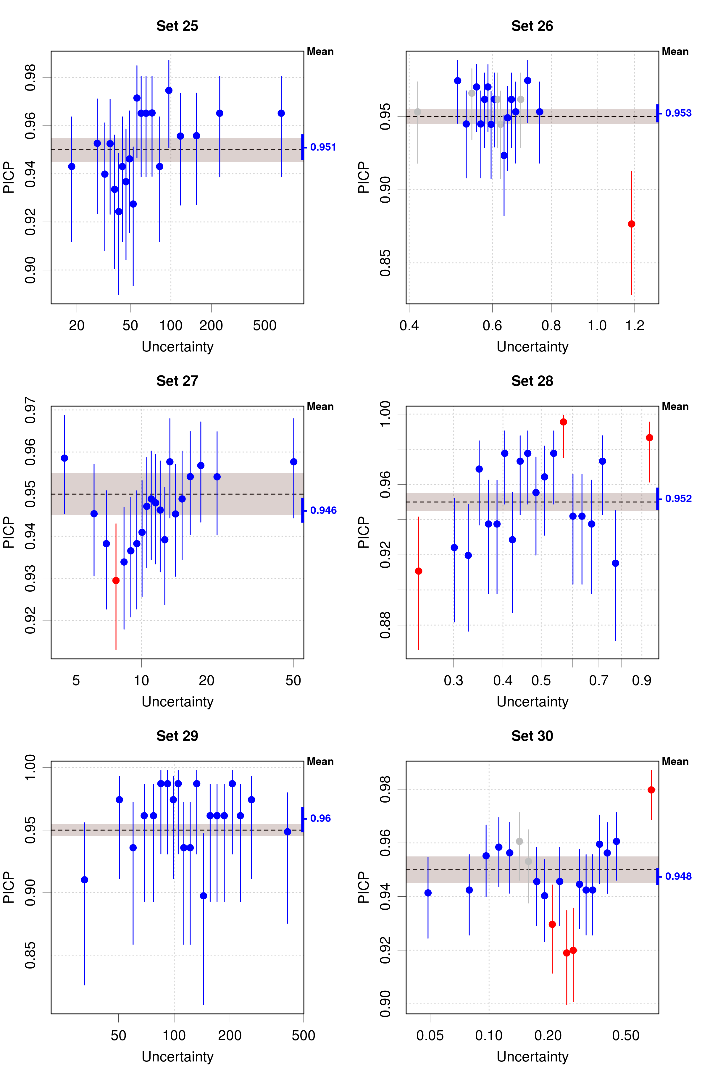
Figure 6: Fig. 4, continued.

IV Conclusions

Using an interval-based metric such as PICP to test prediction uncertainty calibration offers more reliability and less computational burden than using a variance-based metric such as ZMS. It was shown here that interval information can simply be obtained from prediction uncertainty due to the fact that z-scores, even if often heavy-tailed, have mostly scaled Student’s $t_{s}(\nu)$ distributions. The proposed estimation method of PICP at the 95 % level rests on the fact that the $k_{95}$ enlargement factor for $t_{s}(\nu)$ is weakly dependent on $\nu$ and can be fixed at 1.96 with negligible consequences, as long as $\nu>3$. To avoid distribution fitting altogether, testable datasets can be selected by a threshold on a robust skewness metric, i.e. $\beta_{GM}(Z^{2})<0.85$. Unfortunately, this approach is not applicable for other probability levels than 0.95.

Application to the 33 Jacobs et al.’s datasets(Jacobs2024, ) shows that 10 sets have distribution properties (very heavy tails or outliers) making them untestable for average calibration by the PICP (or variance-based: ZMS, NLL, RCE…) metrics. To overcome this limitation, an effort should be done to improve these distributions, for instance by active learning(Pernot2024, ). Among the remaining sets, 18 are validated for average calibration and 5 are not. For the latter, the post-hoc polynomial transformation used by Jacobs et al.(Jacobs2024, ) has not been fully efficient to ensure calibration. Note however, that their PICP values do not exceed 0.97, which might still be considered as acceptable.

Consistency has been tested by the LCP analysis for the 18 calibrated sets, showing that a large majority of them presents adequately uniform local coverage in uncertainty space. Furthermore, this diagnostic might help to improve the post-hoc calibration procedure for the few datasets with local coverage problems.

Author Declarations

Conflict of Interest

The author has no conflicts to disclose.

Code and data availability

The code and data to reproduce the results of this article are available at https://github.com/ppernot/2024_PICP/releases/tag/v1.0 and at Zenodo (https://doi.org/10.5281/zenodo.13373267). The 33 datasets of Jacobs et al.(Jacobs2024, ) are accessible in a FigShare depository(Morgan2024_FigShare, ).

Appendix A Distributions of $Z^{2}$

$Z^{2}$ datasets are fitted by a scaled $F$ distribution, using a maximum goodness-of-fit estimation and the Kolmogorov-Smirnov distance (Delignette2015, ). The results are reported in Figs. 7-12.

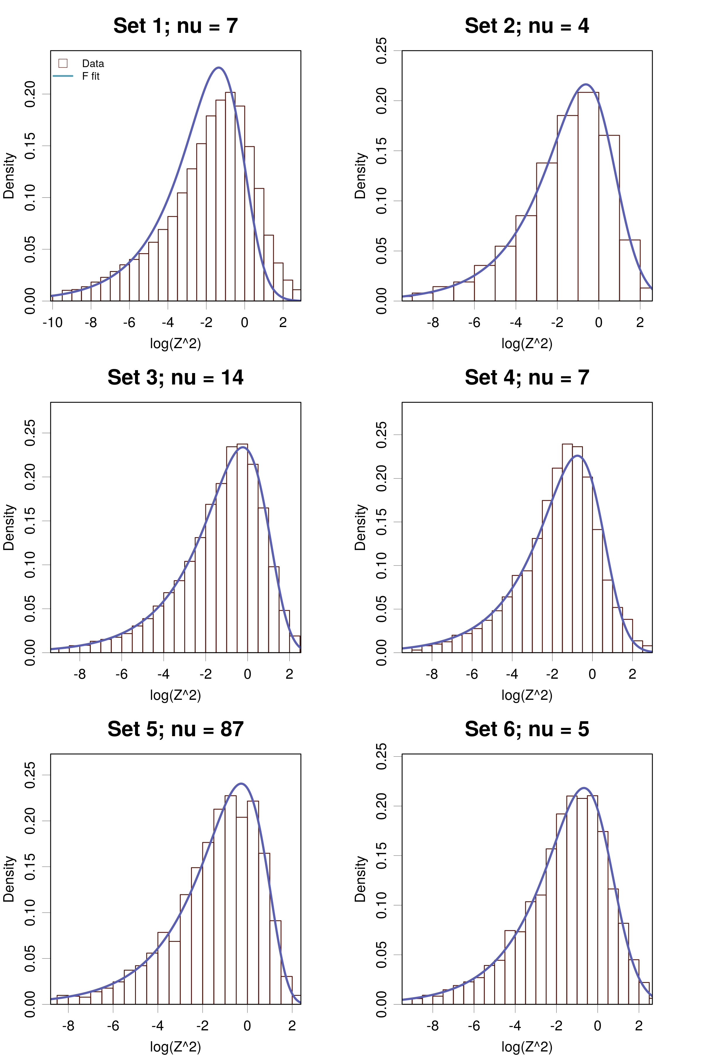
Figure 7: Fit of the squared z-scores (histogram) by a scaled Fisher-Snedecor $F_{s}(1,\nu)$ distribution (blue line). The rounded value of the best-fit shape parameter is reported in the header of each plot.

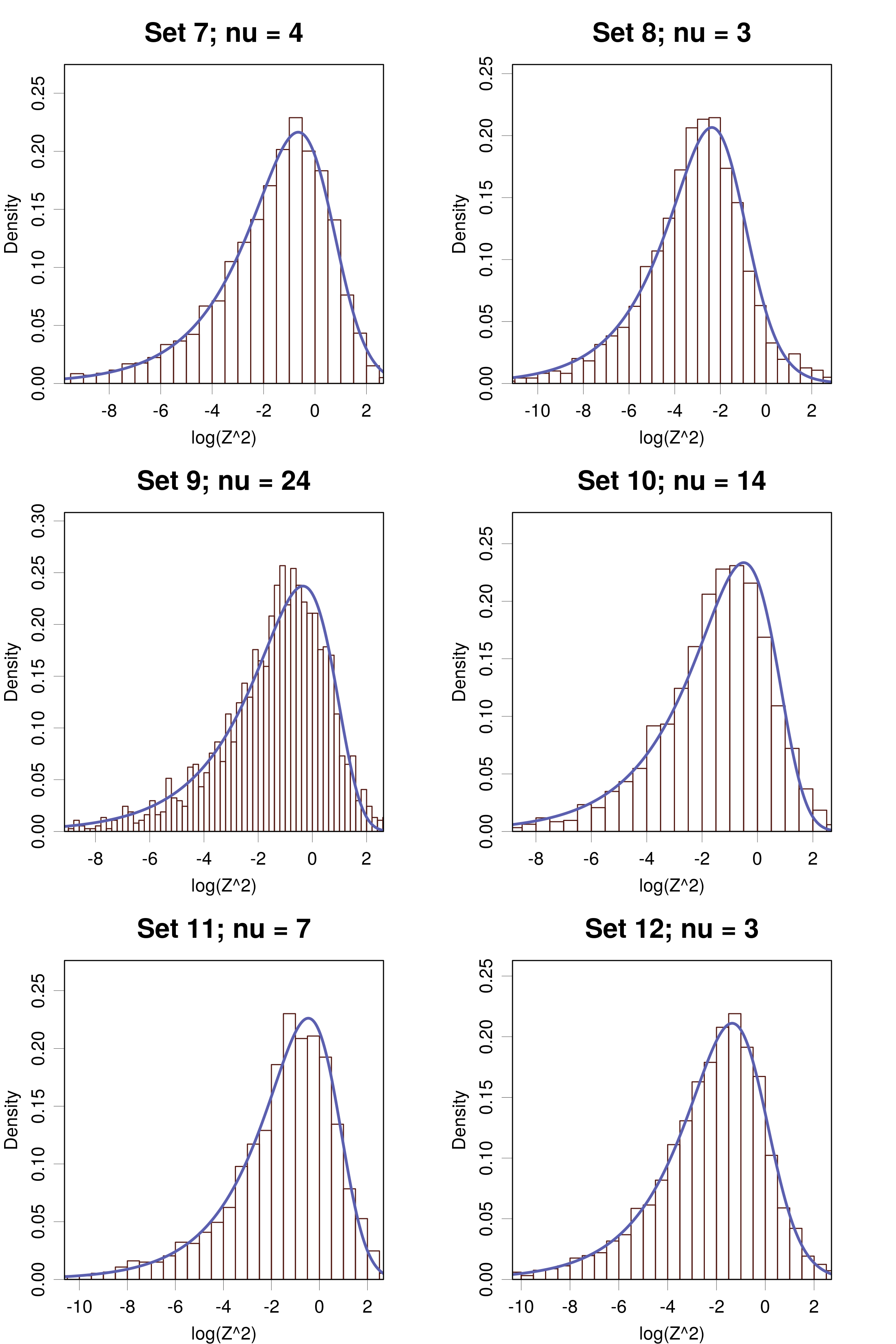
Figure 8: Fig. 7, continued.

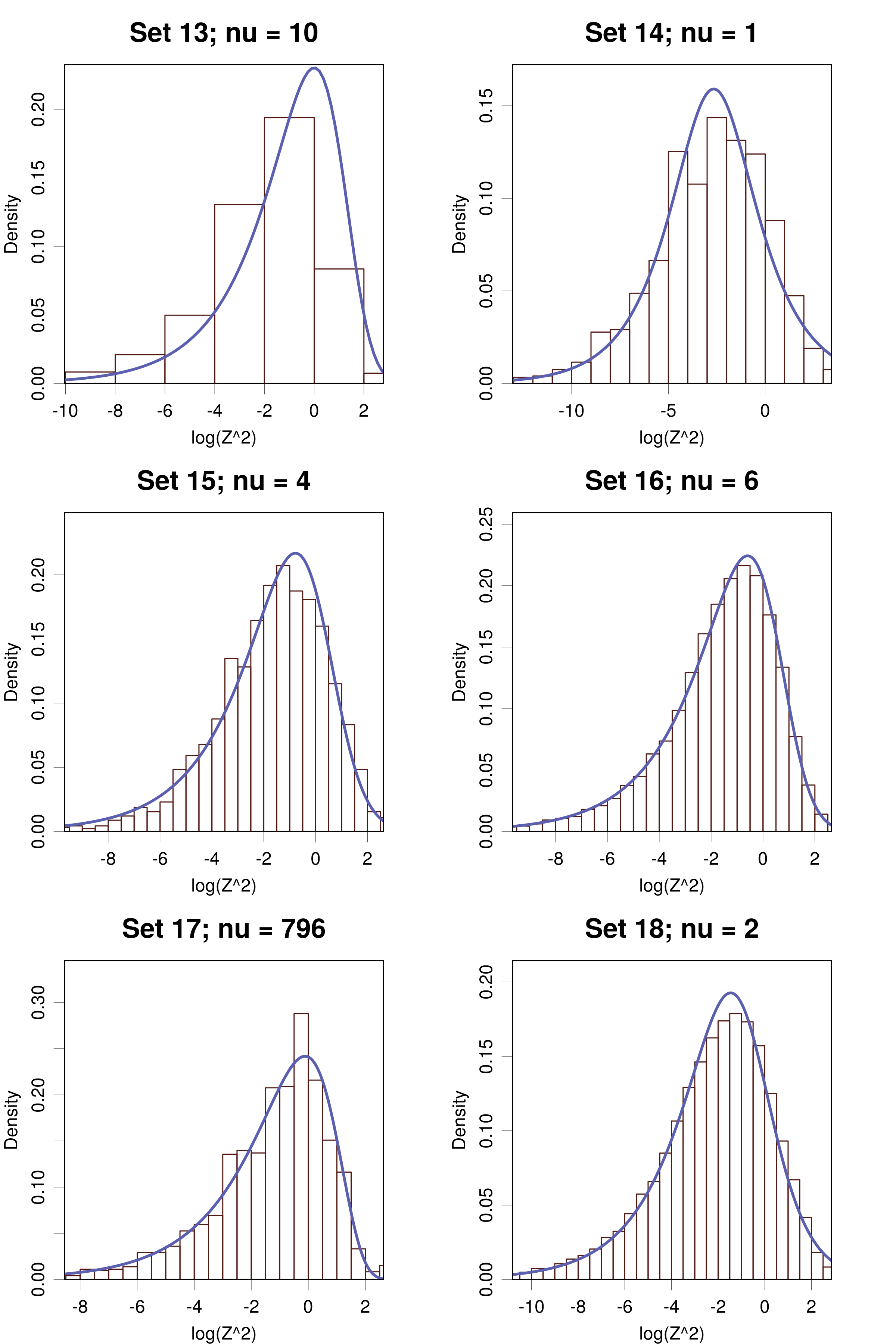
Figure 9: Fig. 7, continued.

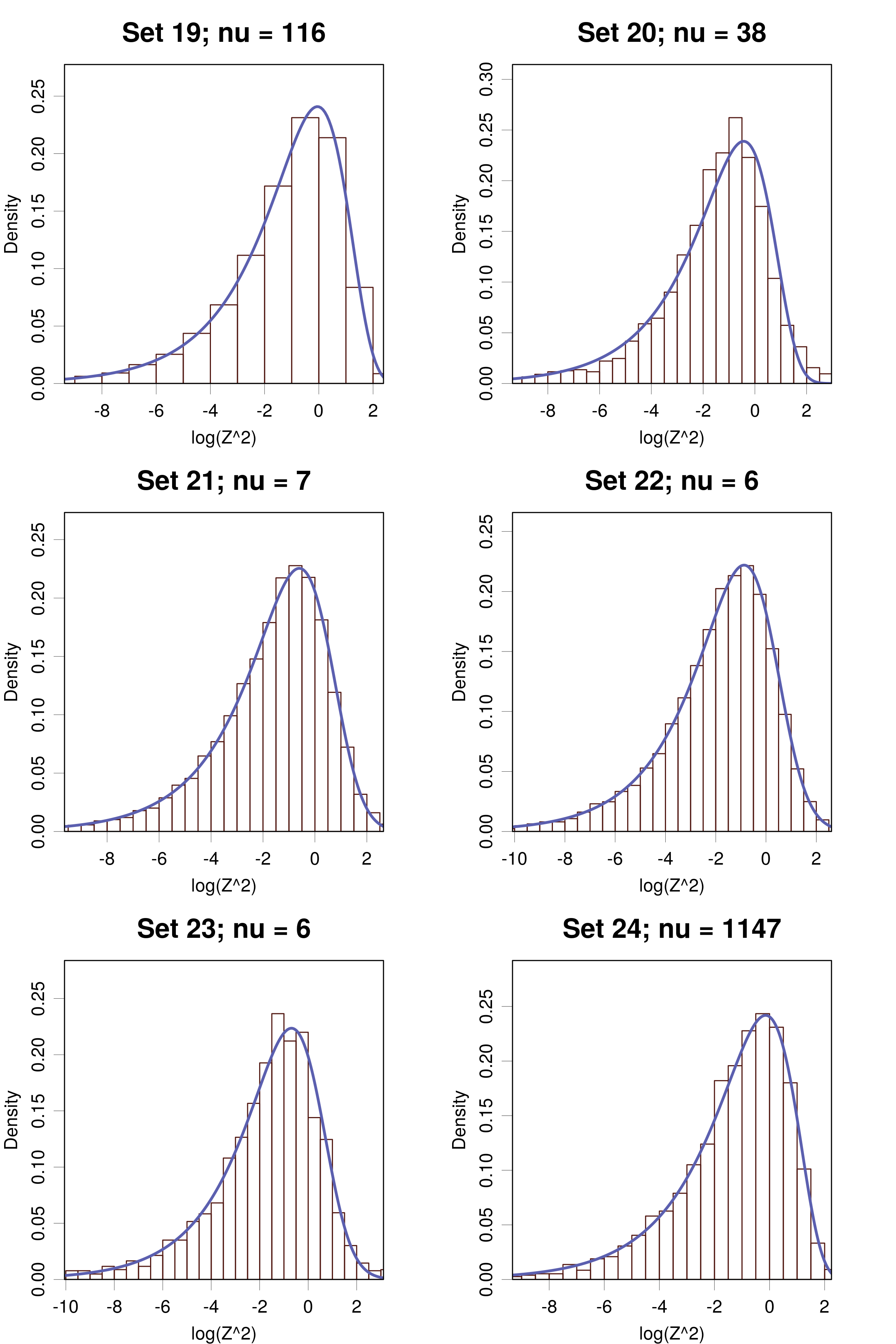
Figure 10: Fig. 7, continued.

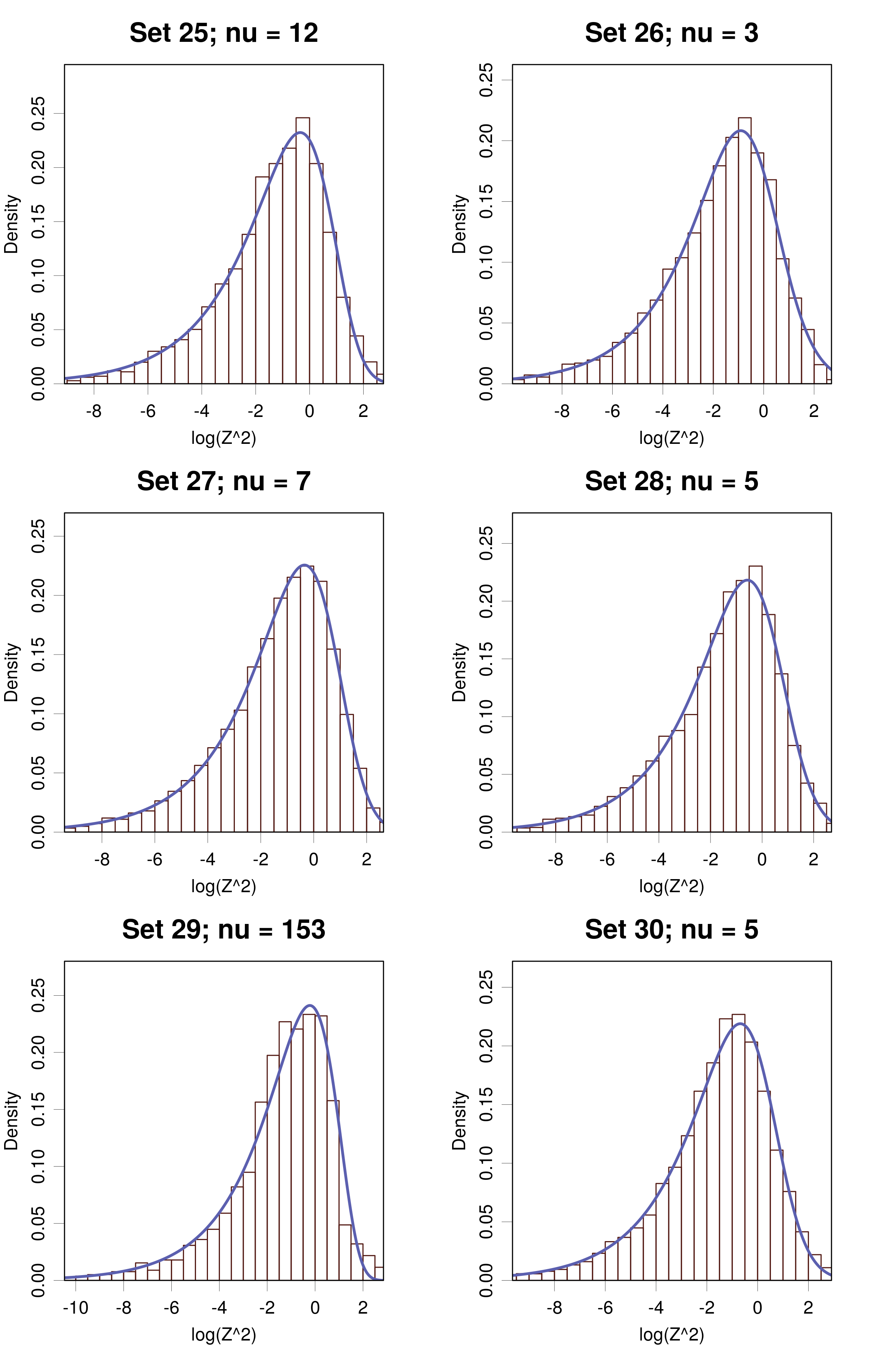
Figure 11: Fig. 7, continued.

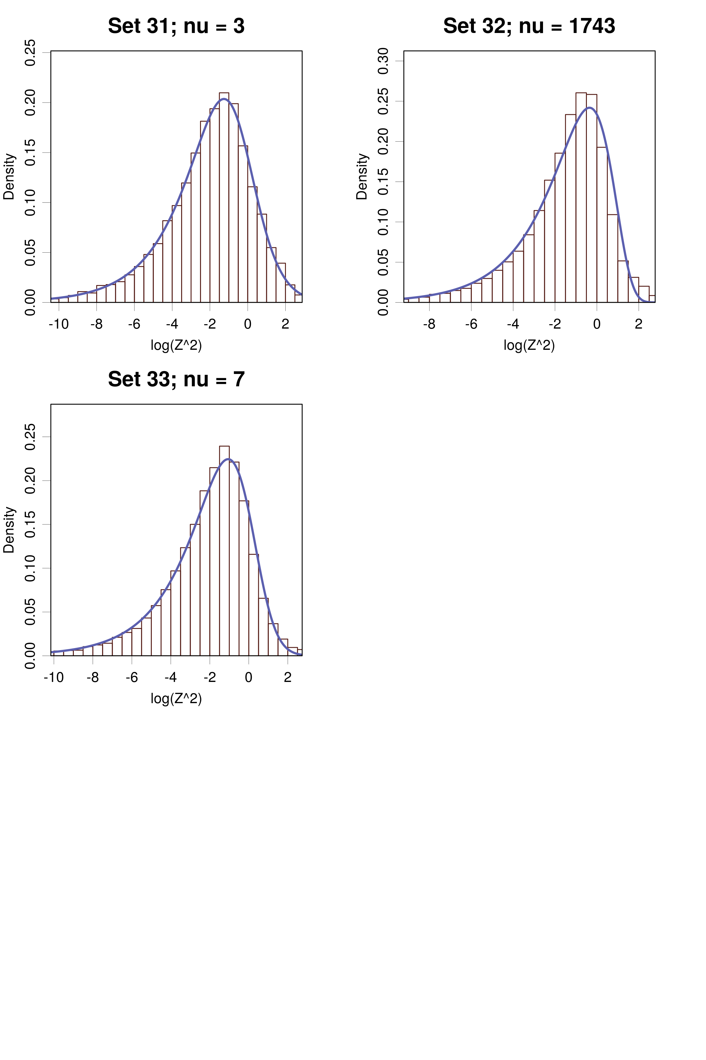
Figure 12: Fig. 7, continued.

References

- (1) P. Pernot. Negative impact of heavy-tailed uncertainty and error distributions on the reliability of calibration statistics for machine learning regression tasks. arXiv:2402.10043, February 2024.
- (2) R. A. Groeneveld and G. Meeden. Measuring skewness and kurtosis. The Statistician, 33:391–399, 1984. URL: http://www.jstor.org/stable/2987742.
- (3) M. Bonato. Robust estimation of skewness and kurtosis in distributions with infinite higher moments. Financ Res Lett, 8:77–87, 2011.
- (4) P. Pernot and A. Savin. Using the Gini coefficient to characterize the shape of computational chemistry error distributions. Theor. Chem. Acc., 140:24, 2021.
- (5) R. Jacobs, L. E. Schultz, A. Scourtas, K. J. Schmidt, O. Price-Skelly, W. Engler, I. Foster, B. Blaiszik, P. M. Voyles, and D. Morgan. Machine Learning Materials Properties with Accurate Predictions, Uncertainty Estimates, Domain Guidance, and Persistent Online Accessibility. arXiv:2406.15650, June 2024.
- (6) P. Pernot. Prediction uncertainty validation for computational chemists. J. Chem. Phys., 157:144103, 2022.
- (7) R. G. Newcombe. Two-sided confidence intervals for the single proportion: comparison of seven methods. Stat. Med., 17:857–872, 1998.
- (8) P. Pernot. The long road to calibrated prediction uncertainty in computational chemistry. J. Chem. Phys., 156:114109, 2022.
- (9) M. Evans, N. Hastings, and B. Peacock. Statistical Distributions. Wiley-Interscience, 3rd edition, 2000.
- (10) M. L. Delignette-Muller and C. Dutang. fitdistrplus: An R package for fitting distributions. J Stat Softw, 64(4):1–34, 2015.
- (11) P. Pernot and F. Cailliez. A critical review of statistical calibration/prediction models handling data inconsistency and model inadequacy. AIChE J., 63:4642–4665, 2017.
- (12) P. Pernot. Calibration in machine learning uncertainty quantification: Beyond consistency to target adaptivity. APL Mach. Learn., 1:046121, 2023.
- (13) D. Morgan and R. Jacobs. Machine Learning Materials Properties with Accurate Predictions, Uncertainty Estimates, Domain Guidance, and Persistent Online Accessibility - FigShare dataset. 6 2024.