Exploring observable effects of scalar operators beyond SMEFT
in the angular distribution of
Abstract
The invariance of the Standard Model Effective Field Theory (SMEFT) imposes relations among different low-energy effective field theory Wilson coefficients (WCs), any deviations from which would signal the presence of physics beyond SMEFT. In this work, we investigate two such relations (, ) among the scalar and the pseudoscalar new-physics WCs that can contribute to processes. We show that, even when new physics violating these relations would not be measurable in the branching ratios of and at HL-LHC and FCC-ee, it can still manifest itself in the angular distribution of . We identify the combinations of angular observables in this decay channel that are sensitive to scenarios beyond SMEFT. We find that the two observables and , and their combination, have the potential to identify physics beyond SMEFT.
I Introduction
Physics beyond the Standard Model (BSM) is often parameterized model-independently in terms of the Standard Model Effective Field Theory (SMEFT) [1, 2]. The effective Lagrangian in SMEFT is written as
| (1) |
Here are the effective operators with mass dimension which are comprised of the Standard Model (SM) fields, and the Wilson coefficients (WCs) encode the corresponding new physics (NP) effects. All the operators in SMEFT are invariant under the SM gauge symmetry .
In flavor physics, the relevant energy scale is near the mass of the meson. At this scale, the heavier particles, i.e. , gauge bosons, the Higgs boson () and the top quark, are integrated out. The resulting effective field theory is the Low-energy Effective Field Theory (LEFT) [3, 4]. As LEFT is relevant below the electroweak (EW) scale, all the operators in LEFT need to be invariant only under . When LEFT operators are matched to SMEFT operators, the invariance of SMEFT imposes several relations among the WCs in LEFT. Such relations and their phenomenological implications have recently been studied in [5, 6, 7, 8, 9, 10, 11, 12, 13, 14, 15, 16, 17, 18, 19, 20, 21, 22, 23, 24].
However, SMEFT is not the only effective field theory (EFT) above the EW scale. There are more general EFTs such as the Higgs Effective Field Theory (HEFT) [25, 26, 27, 28, 29] where the EW symmetry is non-linearly realized. If HEFT is the effective theory above the EW scale, then the relations predicted by SMEFT may no longer be valid. Although SMEFT is a more commonly used EFT in literature, there is no experimental evidence yet to prefer it over HEFT. Searches for beyond-SMEFT physics in ATLAS and CMS focus on the precise measurements of Higgs couplings with fermions and gauge bosons [30]. In this work, our goal is to study the possibility of identifying the effects of physics beyond SMEFT in the channel.
The motivation for focusing on the sector emerges from several recently observed flavor anomalies in meson decays that indicate the possibility of BSM physics. For example, the measurements of [31, 32, 33, 34] and [35] involve the charged-current transition , while the observables [36], [37], [38] and [39, 40, 41] involve the neutral-current transitions . Although these anomalies can be addressed within the framework of SMEFT, the possibility that they originate from physics beyond SMEFT remains open. In our earlier study [42], we have explored the possibility of identifying the beyond-SMEFT effects in the charged-current transition , using angular observables in and constraints from , , .
In this work, we focus on the processes mediated by . In recent literature [43, 44, 45, 46, 12, 20, 47, 24], it has been pointed out that a common explanation of observed excess in and the deviations in the lepton flavor universality (LFU) ratios would predict excess branching fractions for the modes , , etc. It should be noted that, in addition to the branching fractions, the NP will also affect the angular distributions in the modes. In fact, even in the cases where the NP effects are not evident in the branching ratios or are obscured by hadronic uncertainties, they may still show up in the angular distributions. In our analysis, we study the possibility of identifying the NP effects – specifically the effects beyond SMEFT – in the angular observables of , even when they are not measurable in the branching ratios.
Two of the SMEFT predicted relations among the WCs of scalar and pseudoscalar LEFT operators are
| (2) |
We study the possible violation of these relations and the prospects of identifying the physics beyond SMEFT through future measurements of the processes and , which may get contributions from the semileptonic scalar and pseudoscalar operators in the channel.
Currently, the branching ratios of these modes are not well measured. The present experimental bounds are [48], [49] and [50]. These bounds are much weaker as compared to the SM expectations, which are for all these modes [51]. However, these bounds will improve by one or two orders of magnitude in Belle-II [52] and HL-LHC [53]. Moreover, FCC-ee is expected to measure at the SM level with the estimated yield for of in the first two years of running (phase - 1) [54, 55]. This will allow us to carry out angular analyses for these modes.
In this work, we envisage the scenario where the NP effects may not be apparent directly in the branching ratios of and at the level of precision possible at HL-LHC and FCC-ee. Taking these branching ratios to be consistent with the SM, we calculate constraints for the WCs in LEFT contributing to processes based on the projected measurements of these branching ratios. Given these constraints, we explore if the angular observables in are sensitive to any deviations from the SMEFT-predicted relations. We look for combinations of these angular observables that will be able to identify physics beyond SMEFT. Note that angular distributions of have been studied earlier in [56, 57, 58]; however, their potential for identifying beyond-SMEFT effects has not yet been explored.
In Sec. II, we list the effective operators in SMEFT and in LEFT that contribute to the processes and discuss the predictions of SMEFT for the LEFT WCs. In Sec. III, we present the projected constraints on the WCs in LEFT with and without the underlying SMEFT assumptions, taking the NP WCs to be real. In Sec. IV, we discuss the angular observables in and try to identify suitable observables, and their combinations, for distinguishing the scenarios within and beyond SMEFT. In Sec. V, we extend this exercise to the case of complex WCs, pointing out an additional CP-odd observable sensitive to physics beyond SMEFT. Finally, we summarize our results in Sec. VI.
II SMEFT-predicted relations for Wilson coefficients in LEFT
In this section, we list the dimension-6 semileptonic operators in LEFT contributing to the transition at the tree level. Based on the matching of these operators to SMEFT, we present the resulting relations among the WCs in LEFT.
The leading order effective Lagrangian in LEFT for process, considering only semileptonic operators, is [59]
| (3) |
where the operators include the following
| (4) |
Semileptonic operators in SMEFT contributing to channel are
| (5) | ||||
| (6) | ||||
| (7) |
where and are left-handed quark and lepton doublets, whereas and are right-handed down-type quark and right-handed electron, respectively. The matching equations among the WCs of scalar and tensor operators in SMEFT and LEFT are [6, 60]
| (8) | ||||
| (9) | ||||
| (10) |
These matching equations imply the following relations [6, 60, 24]:
| (11) |
These relations result from the conservation of hypercharge in the corresponding SMEFT operators. When considering operators up to dimension 6, these relations hold true irrespective of which SMEFT operators are present at the UV scale. However, in a more general EFT above the EW scale, such as HEFT, the EW gauge symmetry is realized non-linearly, and therefore, the hypercharge need not be conserved in each HEFT operator separately. In this scenario, the resulting LEFT operators may not follow the SMEFT-predicted relations. The matching of LEFT scalar operators to such a non-linear EFT is detailed in [6]:
| (12) |
where is a normalization constant. Here and are the WCs of the corresponding operators and in the non-linear EFT basis in unitary gauge:
| (13) | ||||
| (14) | ||||
| (15) | ||||
| (16) |
Here and correspond to the generation indices for leptons and quarks, respectively. The implication of eq. (12) is that the relations in eq. (11) are no longer maintained. The deviations from the correlations arise due to the WCs and and can be parameterized as
| (17) | ||||
| (18) |
Non-zero values of and indicate effects beyond SMEFT. For the tensor operators, the WCs and are zero in SMEFT, so any nonzero value of these WCs will suggest physics beyond SMEFT. In our numerical analysis, we focus exclusively on the NP vector and scalar operators.
III Constraints on the LEFT WC’s
The NP contributions to transition may arise from the vector and scalar Wilson coefficients , , and . To put constraints on these WCs, we consider the branching ratios and . The SM predictions, current upper bounds and projected future bounds for these modes are presented in Table 1. We envisage the scenario where the NP effects may not be apparent directly in the branching ratios of ; however, they may affect the angular distribution of these decays. Based on these projected measurements, we calculate constraints on the WCs, both in the SMEFT and beyond-SMEFT scenarios.
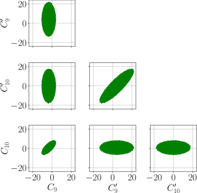
For the WCs associated with the vector operators, the best constraints come from . While constraining these WCs corresponding to the vector operators, we consider the “VA” scenario where we take all the scalar WCs to be zero. Since such events are expected in the phase-I of FCC-ee [54], we project the future precision on conservatively to be within 10% of its SM value. That is, we estimate constraints on the vector WCs with the condition
| (19) |
where stands for . We use the python package flavio [51] to calculate the theoretical prediction for . The resulting constraints on the WCs , , and are shown in Fig. 1.
For the scalar operators, we define
| (20) | ||||
| (21) |
In terms of the above quantities, the SMEFT-predicted relations for the WCs of the scalar operators become
| (22) |
When these relations are obeyed, we call the scenario “SP”. Violations of the SMEFT-predicted relations can be parameterized in terms of the quantities and , where
| (23) |
Note that and can be related to the quantities and defined in eqs. (17) and (18) as
| (24) |
When and/or , we call that scenario as “”. In SP and scenarios, the NP WCs corresponding to the vector operators are taken to be zero.
In [61], current bounds on the scalar operators are calculated indirectly from , processes and directly from , and processes. These bounds are rather weak:
| (25) |


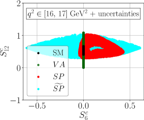
In our analysis, we take , which is the expected upper bound at the HL-LHC and FCC-ee [54], and the expected measurement of at FCC-ee to be within the precision of of the SM value. With these assumptions, we find the allowed region for the four parameters , , and for the two scenarios SP and . We present the projections of these allowed regions in Fig. 2. Note that the observable is more sensitive to and , whereas is more sensitive to and . The upper bound constrains and to a circular cyan region. On the other hand, the constraint on leads to an annular red region in the (, ) plane.
Note that in Fig. 1 and Fig. 2, we have not accounted for uncertainties due to form factors and other input parameters. When these uncertainties are included, the allowed regions broaden, although their overall shapes remain largely unchanged. We shall later include the uncertainties and study their effects.
Based on the allowed WCs values, our next goal is to find observables whose values for the scenario will be distinguishable from those for the VA and SP scenarios.
IV Angular observables in
In this section, we study the effects of the scenario, in comparison to the SM, VA and SP scenarios, on the angular observables in decays. Here and are vector and pseudoscalar mesons, respectively. The angular distribution for decay is given as [62]
| (26) |
where
| (27) |
Here the direction of in the rest frame of B is taken to be the -axis. The angle between the axis and the direction of in the rest frame of V is denoted by . The angle between the axis and the direction of in the center-of-mass frame of the lepton pair is denoted by . The azimuthal angle is the angle between the decay planes formed by the decay products and in the rest frame of . In our analysis, , and .
We calculate the values of the following observables as functions of using the software package flavio [51]:
| (28) |
where and are the corresponding angular coefficient and decay width for the CP-conjugate process. The explicit expressions of these angular observables are available in [62]. In Table 2, we present the observables that are sensitive to each NP parameter.


We calculate these observables in for the SM and the NP scenarios VA, SP and . Note that when we calculate the expected values of the observables in the VA scenario, we consider points for and from the allowed regions as shown in Fig. 1, while keeping all WCs for the scalar operators as zero. Similarly, while calculating observables in SP () scenario, we put and take points from the red (cyan) regions shown in Fig. 2. We find that the angular observables , , and show significant sensitivity to the SP and scenarios. In Fig. 3, we present the expected values of , and in SM and in the NP scenarios VA, SP and . For all these four observables, we have considered uncertainties due to form factors and other input parameters, and the WCs corresponding to the NP scenarios are varied within their allowed regions.
| NP WCs | Sensitive observables |
| , | , , , , , , , |
| , , | |
| , |
As shown in Fig. 3, the observables and by themselves would not be able to distinguish the effects of from VA and SP scenarios or even from the SM. However, the observable is suppressed for both SM and VA and may have significant nonzero values for SP and scenarios. Moreover, some values of that are possible in are not achievable in SP scenario. Thus is a good probe for distinguishing between scenarios within SMEFT (VA and SP) and beyond SMEFT (). For example, even a small negative value of will hint towards physics beyond SMEFT.


Next, we ask whether it is possible to distinguish the different scenarios even in the case of having a positive value. To answer this, we consider the pairs of angular observables (, ) and (, ). The left panels of Fig. 4 show the possible points in the respective planes for a fixed value of and in the absence of any uncertainties in the input parameters. This indicates that in principle the combination with another observable would be more efficient than alone in identifying the beyond-SMEFT effects. However, the necessity of binning over reduces the efficacy of such combinations as shown in the central panels of Fig. 4. The inclusion of uncertainties due to form factors and input parameters further limits the ability of these combinations of observables as probes of physics beyond SMEFT. This may be seen from the right panels of Fig. 4. Thus, one would need narrow bins (hence a large number of events) and better control over theory parameters in order to effectively exploit such combinations.
V Results with complex NP Wilson coefficients
In our analysis so far, we have considered all the WCs to be real. However, the WCs in LEFT can be complex in general. Note that even if all the WCs in SMEFT (or HEFT) in the UV scale are real in the flavor basis, phases will appear in low-energy WCs through CKM elements while matching. The basic idea and results of our analysis are independent of whether the WCs are real or complex. However, it is worthwhile to see the effects of complex WCs on the angular observables, especially the ones that are asymmetric under charge-parity (CP) transformation.
In this section, we consider the WCs , , and to be complex. In Fig. 5, we present the allowed regions for complex and in the VA scenario. The methodology for obtaining these constraints is the same as discussed in Sec. III. Note that we allow all of these parameters to be nonzero at the same time, however, we do not show the correlations among them in Fig. 5. The regions are symmetric about the real axis as expected.
In Fig. 6, we show the allowed regions for complex and in the SP and scenarios. It is observed that the allowed regions in and parameter spaces in the two scenarios SP and overlap almost completely. However, for and , there are regions in this complex parameter space that are only accessible in the scenario beyond SMEFT ().


The results for the observables , , and are similar to the ones discussed in Sec. IV with allowed regions becoming wider. We do not show the results with these individual observables in this section. The results for the combinations (, ) and (,, ) are shown in Fig. 7. These indicate that for complex WCs, a significantly negative value of () as well as a large positive value of () would suggest physics beyond SMEFT. The observables and do not seem to be offering any extra advantage to identify .


We further explore the CP asymmetric observable defined as
| (29) |
In the SM as well as in the NP scenarios where all the WCs are real, is highly suppressed. However, for complex WCs, it may become significantly nonzero. The value of this observable as a function of is shown in the top panel of Fig. 8. Clearly, has the ability to identify the scenario by itself. The combination of and can be more effective at this task than the two observables separately, even after taking into account the binning of GeV2 and theoretical uncertainties, as can be seen in the bottom panel of Fig. 8.


VI Concluding remarks
The Standard Model effective field theory (SMEFT) is often taken to be the default EFT above the EW scale. However, more general EFTs, such as Higgs effective field theory (HEFT) where the EW gauge symmetry is non-linearly realized, are still not ruled out. In this paper, we study the possibility of probing beyond-SMEFT physics in low-energy processes mediated via the transition.
When relevant operators in the low-energy effective field theory (LEFT) are mapped to the EFT above the EW scale, certain relations that are satisfied in SMEFT may not hold if a more general EFT such as HEFT is valid over the EW scale. For the neutral-current transition , some such relations are , , which are predicted by SMEFT. We identify observables that are sensitive to any deviations from these relations and explore the possibility of distinguishing these deviations from not only SM, but also from other NP scenarios that are still within SMEFT.
We consider three NP scenarios (i) VA, where only NP vector operators are nonzero, (ii) SP, where only NP scalar operators are nonzero but SMEFT-predicted relations are obeyed, and (iii) , where only NP scalar operators are nonzero and the SMEFT-predicted relations are not imposed. We calculate constraints on the NP WCs in these three scenarios using projected observations of and with the precision expected in HL-LHC and the phase-I of FCC-ee. We take these measurements to be consistent with the SM; specifically, we consider an upper bound and a measurement of within 10% of its SM prediction.
We calculate the values of angular observables in , as functions of , in the SM and the three NP scenarios mentioned above, possible with the allowed real values of the NP WCs. We find that the angular observable will be the most efficient in distinguishing the beyond-SMEFT scenario from the SM as well as from the other NP scenarios. A significant negative value of or a large positive value of would suggest physics beyond SMEFT. The observables and can help in this identification in principle. However, with a 1 GeV2 binning in and the inclusion of current theoretical uncertainties, the usefulness of these observables would seem rather constrained.


We further consider the possibility that the NP WCs can take complex values and repeat the above analysis. This allows us to access an additional angular observable which is sensitive to beyond-SMEFT effects. Moreover, the combination of and would be more effective compared to the two observables by themselves. Thus, we demonstrate that the NP that would be hidden if we only looked at the branching ratios could manifest itself in these angular observables.
Although the measurements of the two branching ratios considered in our analysis will only be available after the full run of HL-LHC (for ) and phase-I of FCC-ee (for ), the analysis proposed is a promising way to identify scenarios beyond SMEFT through neutral-current semileptonic decays of mesons and underscores the importance of efficient detection in future collider experiments.
Acknowledgements
We would like to thank Susobhan Chattopadhyay, Rick S. Gupta, Gagan B. Mohanty and Tuhin S. Roy for useful discussions. This work is supported by the Department of Atomic Energy, Government of India, under Project Identification Number RTI 4002. We acknowledge the use of computational facilities of the Department of Theoretical Physics at Tata Institute of Fundamental Research, Mumbai. We would also like to thank Ajay Salve and Kapil Ghadiali for technical assistance.
Appendix A The angular observable
In Table 2 we have mentioned that the observable is sensitive to . Indeed, it gets a contribution from at the leading order while the contributions from and the vector WCs are suppressed by a factor of . In this appendix, we study the effectiveness of in distinguishing the scenario from SM and the other NP scenarios. We present this observable separately because it is not directly available in flavio.
We calculate following the expressions in [62] and taking the form factors from [63]. We consider the scenario where all the NP WCs are real. It is observed that by itself will not be able to distinguish the scenario from SP, though it can distinguish it from VA. The combination of and could offer an advantage over these two observables separately in certain regions of parameter space. This may be seen in Fig. 9.
It may be worthwhile to comment on the observable in the context of . In this case, the contributions from and the vector WCs are strongly suppressed, i.e., by . However, since the NP WCs in are severely constrained [64], it would not be possible to identify the beyond-SMEFT scenario in the muon mode with the analysis proposed in this article.
References
- [1] B. Grzadkowski, M. Iskrzynski, M. Misiak and J. Rosiek, Dimension-Six Terms in the Standard Model Lagrangian, JHEP 10 (2010) 085 [arXiv:1008.4884].
- [2] G. Isidori, F. Wilsch and D. Wyler, The Standard Model effective field theory at work, [arXiv:2303.16922].
- [3] G. Buchalla, A.J. Buras and M.E. Lautenbacher, Weak decays beyond leading logarithms, Rev. Mod. Phys. 68 (1996) 1125 [hep-ph/9512380].
- [4] E.E. Jenkins, A.V. Manohar and P. Stoffer, Low-Energy Effective Field Theory below the Electroweak Scale: Operators and Matching, JHEP 03 (2018) 016 [arXiv:1709.04486].
- [5] R. Alonso, B. Grinstein and J. Martin Camalich, gauge invariance and the shape of new physics in rare decays, Phys. Rev. Lett. 113 (2014) 241802 [arXiv:1407.7044].
- [6] O. Catà and M. Jung, Signatures of a nonstandard Higgs boson from flavor physics, Phys. Rev. D 92 (2015) 055018 [arXiv:1505.05804].
- [7] A. Azatov, D. Bardhan, D. Ghosh, F. Sgarlata and E. Venturini, Anatomy of anomalies, JHEP 11 (2018) 187 [arXiv:1805.03209].
- [8] J. Fuentes-Martin, A. Greljo, J. Martin Camalich and J.D. Ruiz-Alvarez, Charm physics confronts high-pT lepton tails, JHEP 11 (2020) 080 [arXiv:2003.12421].
- [9] R. Bause, H. Gisbert, M. Golz and G. Hiller, Lepton universality and lepton flavor conservation tests with dineutrino modes, Eur. Phys. J. C 82 (2022) 164 [arXiv:2007.05001].
- [10] R. Bause, H. Gisbert, M. Golz and G. Hiller, Rare charm dineutrino null tests for machines, Phys. Rev. D 103 (2021) 015033 [arXiv:2010.02225].
- [11] S. Bißmann, C. Grunwald, G. Hiller and K. Kröninger, Top and Beauty synergies in SMEFT-fits at present and future colliders, JHEP 06 (2021) 010 [arXiv:2012.10456].
- [12] R. Bause, H. Gisbert, M. Golz and G. Hiller, Interplay of dineutrino modes with semileptonic rare B-decays, JHEP 12 (2021) 061 [arXiv:2109.01675].
- [13] R. Bause, H. Gisbert-Mullor, M. Golz and G. Hiller, Dineutrino modes probing lepton flavor violation, PoS EPS-HEP2021 (2022) 563 [arXiv:2110.08795].
- [14] S. Bruggisser, R. Schäfer, D. van Dyk and S. Westhoff, The Flavor of UV Physics, JHEP 05 (2021) 257 [arXiv:2101.07273].
- [15] R. Bause, H. Gisbert, M. Golz and G. Hiller, Model-independent analysis of processes, Eur. Phys. J. C 83 (2023) 419 [arXiv:2209.04457].
- [16] S. Sun, Q.-S. Yan, X. Zhao and Z. Zhao, Constraining rare B decays by +-→tc at future lepton colliders, Phys. Rev. D 108 (2023) 075016 [arXiv:2302.01143].
- [17] C. Grunwald, G. Hiller, K. Kröninger and L. Nollen, More synergies from beauty, top, Z and Drell-Yan measurements in SMEFT, JHEP 11 (2023) 110 [arXiv:2304.12837].
- [18] A. Greljo, J. Salko, A. Smolkovič and P. Stangl, SMEFT restrictions on exclusive b → u decays, JHEP 11 (2023) 023 [arXiv:2306.09401].
- [19] S. Fajfer, J.F. Kamenik and I. Nisandzic, On the Sensitivity to New Physics, Phys. Rev. D 85 (2012) 094025 [arXiv:1203.2654].
- [20] R. Bause, H. Gisbert and G. Hiller, Implications of an enhanced B→K¯ branching ratio, Phys. Rev. D 109 (2024) 015006 [arXiv:2309.00075].
- [21] S. Bhattacharya, S. Jahedi, S. Nandi and A. Sarkar, Probing flavour constrained SMEFT operators through production at the Muon collider, [arXiv:2312.14872].
- [22] F.-Z. Chen, Q. Wen and F. Xu, Correlating and flavor anomalies in SMEFT, [arXiv:2401.11552].
- [23] E. Fernández-Martínez, X. Marcano and D. Naredo-Tuero, Global Lepton Flavour Violating Constraints on New Physics, [arXiv:2403.09772].
- [24] S. Karmakar, A. Dighe and R.S. Gupta, SMEFT predictions for semileptonic processes, [arXiv:2404.10061].
- [25] R. Alonso, M.B. Gavela, L. Merlo, S. Rigolin and J. Yepes, The Effective Chiral Lagrangian for a Light Dynamical ”Higgs Particle”, Phys. Lett. B 722 (2013) 330 [arXiv:1212.3305].
- [26] G. Buchalla, O. Catà and C. Krause, Complete Electroweak Chiral Lagrangian with a Light Higgs at NLO, Nucl. Phys. B 880 (2014) 552 [arXiv:1307.5017].
- [27] A. Pich, I. Rosell, J. Santos and J.J. Sanz-Cillero, Fingerprints of heavy scales in electroweak effective Lagrangians, JHEP 04 (2017) 012 [arXiv:1609.06659].
- [28] T. Cohen, N. Craig, X. Lu and D. Sutherland, Is SMEFT Enough?, JHEP 03 (2021) 237 [arXiv:2008.08597].
- [29] C.P. Burgess, S. Hamoudou, J. Kumar and D. London, Beyond the standard model effective field theory with , Phys. Rev. D 105 (2022) 073008 [arXiv:2111.07421].
- [30] J. Alison et al., Higgs boson potential at colliders: Status and perspectives, Rev. Phys. 5 (2020) 100045 [arXiv:1910.00012].
- [31] BaBar collaboration, Evidence for an excess of decays, Phys. Rev. Lett. 109 (2012) 101802 [arXiv:1205.5442].
- [32] BaBar collaboration, Measurement of an Excess of Decays and Implications for Charged Higgs Bosons, Phys. Rev. D 88 (2013) 072012 [arXiv:1303.0571].
- [33] Belle collaboration, Measurement of the branching ratio of relative to decays with hadronic tagging at Belle, Phys. Rev. D 92 (2015) 072014 [arXiv:1507.03233].
- [34] LHCb collaboration, Measurement of the ratio of branching fractions , Phys. Rev. Lett. 115 (2015) 111803 [arXiv:1506.08614].
- [35] LHCb collaboration, Measurement of the ratio of branching fractions /, Phys. Rev. Lett. 120 (2018) 121801 [arXiv:1711.05623].
- [36] LHCb collaboration, Differential branching fractions and isospin asymmetries of decays, JHEP 06 (2014) 133 [arXiv:1403.8044].
- [37] LHCb collaboration, Measurement of lepton universality parameters in and decays, [arXiv:2212.09153].
- [38] Belle-II collaboration, Evidence for Decays, [arXiv:2311.14647].
- [39] LHCb collaboration, Measurement of Form-Factor-Independent Observables in the Decay , Phys. Rev. Lett. 111 (2013) 191801 [arXiv:1308.1707].
- [40] S. Descotes-Genon, J. Matias, M. Ramon and J. Virto, Implications from clean observables for the binned analysis of at large recoil, JHEP 01 (2013) 048 [arXiv:1207.2753].
- [41] S. Descotes-Genon, J. Matias and J. Virto, Understanding the Anomaly, Phys. Rev. D 88 (2013) 074002 [arXiv:1307.5683].
- [42] S. Karmakar, S. Chattopadhyay and A. Dighe, Identifying physics beyond SMEFT in the angular distribution of b→c(→)¯ decay, Phys. Rev. D 110 (2024) 015010 [arXiv:2305.16007].
- [43] R. Alonso, B. Grinstein and J. Martin Camalich, Lepton universality violation and lepton flavor conservation in -meson decays, JHEP 10 (2015) 184 [arXiv:1505.05164].
- [44] A. Crivellin, D. Müller and T. Ota, Simultaneous explanation of R(D(∗)) and b→s+ -: the last scalar leptoquarks standing, JHEP 09 (2017) 040 [arXiv:1703.09226].
- [45] L. Calibbi, A. Crivellin and T. Li, Model of vector leptoquarks in view of the -physics anomalies, Phys. Rev. D 98 (2018) 115002 [arXiv:1709.00692].
- [46] B. Capdevila, A. Crivellin, S. Descotes-Genon, L. Hofer and J. Matias, Searching for New Physics with processes, Phys. Rev. Lett. 120 (2018) 181802 [arXiv:1712.01919].
- [47] L. Allwicher, D. Becirevic, G. Piazza, S. Rosauro-Alcaraz and O. Sumensari, Understanding the first measurement of B(B→K¯), Phys. Lett. B 848 (2024) 138411 [arXiv:2309.02246].
- [48] LHCb collaboration, Search for the decays and , Phys. Rev. Lett. 118 (2017) 251802 [arXiv:1703.02508].
- [49] BaBar collaboration, Search for at the BaBar experiment, Phys. Rev. Lett. 118 (2017) 031802 [arXiv:1605.09637].
- [50] Belle collaboration, Search for the decay B0→K*0+- at the Belle experiment, Phys. Rev. D 108 (2023) L011102 [arXiv:2110.03871].
- [51] D.M. Straub, flavio: a Python package for flavour and precision phenomenology in the Standard Model and beyond, [arXiv:1810.08132].
- [52] Belle-II collaboration, The Belle II Physics Book, PTEP 2019 (2019) 123C01 [arXiv:1808.10567].
- [53] LHCb collaboration, Physics case for an LHCb Upgrade II - Opportunities in flavour physics, and beyond, in the HL-LHC era, [arXiv:1808.08865].
- [54] FCC collaboration, FCC Physics Opportunities: Future Circular Collider Conceptual Design Report Volume 1, Eur. Phys. J. C 79 (2019) 474.
- [55] A. Apollonio et al., FCC-ee Operation Model, Availability & Performance, in 62nd ICFA Advanced Beam Dynamics Workshop on High Luminosity Circular Colliders, p. WEPAB03, JACOW, 2019, DOI.
- [56] T.M. Aliev and M. Savci, Lepton polarization and CP violating effects in decay in standard and two Higgs doublet models, Phys. Lett. B 481 (2000) 275 [hep-ph/0003188].
- [57] S.R. Choudhury, N. Gaur, A.S. Cornell and G.C. Joshi, Lepton polarization correlations in , Phys. Rev. D 68 (2003) 054016 [hep-ph/0304084].
- [58] N.R. Singh Chundawat, New physics in : A model independent analysis, Phys. Rev. D 107 (2023) 055004 [arXiv:2212.01229].
- [59] D. Das, On the angular distribution of decay, JHEP 07 (2018) 063 [arXiv:1804.08527].
- [60] J. Aebischer, A. Crivellin, M. Fael and C. Greub, Matching of gauge invariant dimension-six operators for and transitions, JHEP 05 (2016) 037 [arXiv:1512.02830].
- [61] C. Bobeth and U. Haisch, New Physics in : () Operators, Acta Phys. Polon. B 44 (2013) 127 [arXiv:1109.1826].
- [62] W. Altmannshofer, P. Ball, A. Bharucha, A.J. Buras, D.M. Straub and M. Wick, Symmetries and Asymmetries of Decays in the Standard Model and Beyond, JHEP 01 (2009) 019 [arXiv:0811.1214].
- [63] A. Bharucha, D.M. Straub and R. Zwicky, in the Standard Model from light-cone sum rules, JHEP 08 (2016) 098 [arXiv:1503.05534].
- [64] F. Beaujean, C. Bobeth and S. Jahn, Constraints on tensor and scalar couplings from and , Eur. Phys. J. C 75 (2015) 456 [arXiv:1508.01526].