Constructing Tight Quadratic Relaxations for Global Optimization: II. Underestimating Difference-of-Convex (D.C.) Functions
Abstract
Recent advances in the efficiency and robustness of algorithms solving convex quadratically constrained quadratic programming (QCQP) problems motivate developing techniques for creating convex quadratic relaxations that, although more expensive to compute, provide tighter bounds than their classical linear counterparts. In the first part of this two-paper series [Strahl et al., 2024], we developed a cutting plane algorithm to construct convex quadratic underestimators for twice-differentiable convex functions, which we extend here to address the case of non-convex difference-of-convex (d.c.) functions as well. Furthermore, we generalize our approach to consider a hierarchy of quadratic forms, thereby allowing the construction of even tighter underestimators. On a set of d.c. functions extracted from benchmark libraries, we demonstrate noteworthy reduction in the hypervolume between our quadratic underestimators and linear ones constructed at the same points. Additionally, we construct convex QCQP relaxations at the root node of a spatial branch-and-bound tree for a set of systematically created d.c. optimization problems in up to four dimensions, and we show that our relaxations reduce the gap between the lower bound computed by the state-of-the-art global optimization solver BARON and the optimal solution by an excess of 90%, on average.
Keywords: deterministic global optimization, convex relaxation, quadratic underestimation, cutting-plane algorithm, difference-of-convex (d.c.) functions
1 Introduction
Global optimization is utilized in a variety of research fields, including recent applications in route planning for unmanned air vehicles [Öztürk and Köksalan, 2023], energy storage system selection, design, and operation [Zantye et al., 2023], heat exchanger network synthesis [Zhou et al., 2024], resource recovery from wastewater [Durkin et al., 2024], pathway optimization using kinetic metabolic models for mammalian cells [Lu et al., 2023], profit maximization of scheduling hydrogen production with solar power and grid energy supply [Yang et al., 2022], and minimizing nitrogen oxide emissions produced by incinerating explosive waste materials [Kim et al., 2022], to name but a few. The interested reader can find a plethora of additional historical applications of global optimization in eleven different research areas nicely organized in Table 2 of Boukouvala et al. [2016]. Indeed, the ubiquitous utilization of global optimization in the literature manifests its substantial impact as a tool for scientific discovery and also highlights the importance of any advancements in this area.
The key feature of global optimization algorithms is their guarantee for identification of a global–rather than local–optimal solution. In contrast to optimization problems that are convex (i.e, the objective function and the feasible set are convex), for which a local minimum is also global [Bertsekas et al., 2003], non-convex problems exhibit additional complexity in the sense that non-convex objective surfaces and constraints and/or disjoint feasible regions lead to the existence of multiple extrema. For such problems, many global optimization algorithms, such as spatial branch-and-bound, compute rigorous lower and upper bounds on the objective value and successively refine those on partitioned space until the bounds converge (within some tolerance) to a global optimal solution. Without question, the quality of the bounds impacts the convergence of these algorithms.
For minimization problems, the objective function evaluated at any feasible solution provides an upper bound, while the globally optimal objective value of a relaxation of the problem provides a lower bound. Convex relaxations find extensive applications in these algorithms for determining lower bounds because their local (and hence global) minimum are efficient to compute; also, the quality of the convex relaxation used (i.e., how closely the convex relaxation approximates the original problem) directly impacts the quality of the computed bound. To this end, an enormous amount of research has focused on developing tight convex relaxations for various specific problem structures, which has entailed significant work on deriving convex envelopes for many types of functions. Additionally, after the required expense to construct the relaxations, algorithms available to solve the convex relaxation, such as linear programming (LP) or non-linear programming (NLP) solvers, contribute to the effort required to determine the bound, and thereby contribute greatly to the overall efficiency of the algorithm. Noting the improvement in the robustness and efficiency of algorithms that solve convex quadratically constrained quadratic programs (QCQPs) [Mittelmann, 2023], we focus in this work on creating tight convex quadratic relaxations of non-convex optimization problems. In particular, we extend our previous methodology for constructing quadratic outer approximations of twice-differentiable convex functions [Strahl et al., 2024] to the case of non-convex difference-of-convex (d.c.) functions, which is a very general class of functions arising ubiquitously in global optimization applications.
In the literature, quadratics are frequently utilized to create convex relaxations of non-convex functions, but in most cases they do not result in an actual quadratic relaxation. The BB methodology, for example, uses quadratics to create convex relaxations for general non-convex functions by adding a sufficiently large convex quadratic term to overcome the non-convexities of the function over the entire domain [Maranas and Floudas, 1995, Androulakis et al., 1995, Adjiman et al., 1998b, b]. The approach has been generalized in Akrotirianakis et al. [2004], Skjäl et al. [2012] to include modifications to the diagonal and nondiagonal terms of the quadratic, extended in Meyer and Floudas [2005] to use subintervals of the domain to create a spline from piecewise quadratic functions, and utilized in Gounaris and Floudas [2008a, b] to create tight piecewise linear convex relaxations for non-convex functions. While the BB methodology utilizes quadratics in the construction of underestimators, it only creates a quadratic underestimator if the function that is underestimated is itself quadratic. Excluding this special case, none of the BB variants discussed above produce create convex quadratic relaxations.
Other studies in the literature have proposed quadratic underestimators for convex functions, but these works restrict construction of their underestimators to specific classes of functions or problems. Su et al. [2018] proposed scaling the second-order term of a Taylor series approximation at a point of construction and provided a procedure for determining the tightest scaling parameter for underestimating a restrictive class of functions, which has been the foundational study for our own work. Buchheim and Trieu [2013] use quadratic underestimators in integer programming, introducing quadratic cuts that are generated for a specific class of functions where a matrix, , is known a priori to satisfy for all . Olama et al. [2023] includes quadratic cuts in a mixed integer nonlinear programming algorithm derived specifically for strongly convex functions where the strong convexity parameter is easily determined. Last, there exist studies in the literature that construct quadratic underestimators for general non-convex functions, but these procedures either lack guarantees of convexity for the quadratic underestimators, or they only apply in restricted contexts. In particular, Streeter and Dillon [2022, 2023] introduce quadratic over- and underestimators for general functions based on so-called Taylor polynomial enclosures, which are efficiently constructed even for functions of high dimension, but are not guaranteed to be convex. In their work, Ouanes et al. [2015] present a procedure to create a convex quadratic underestimator by subtracting a quadratic perturbation from a linear interpolant of a general non-convex function, but their method only applies in the restricted context of minimizing a single multivariate function subject to box constraints.
As discussed, in this paper we will focus on underestimating d.c. functions. The importance of such functions in optimization is evidenced by their extensive appearance in the literature, which is due to their general applicability, succinctly captured by Tuy’s statement that “every continuous global optimization problem on a compact set can be reformulated as a d.c. optimization problem” in Horst and Pardalos [2013] (pp. 149-150). In fact, early pioneers established that any twice-differentiable continuous function defined over a convex set in is representable as a d.c. function [Hartman, 1959], and a later study showed that any piecewise linear continuous function can be expressed as a d.c. function too [Melzer, 1986]. Difference-of-convex functions naturally arise in a diverse number of specific applications, including but not limited to problems in signal processing, communications, and networking [Gasso et al., 2009, Alvarado et al., 2014, Nguyen and Le Thi, 2023], transportation [Holmberg and Tuy, 1999], facility location [Chen et al., 1998], image processing [Lou et al., 2015], clustering [Bagirov et al., 2016, Bagirov and Ugon, 2018], and machine learning [Le Thi and Nguyen, 2017, Awasthi et al., 2024, Askarizadeh et al., 2023].
Relaxations for d.c. functions exist in the literature, but they are not convex quadratic, except in limited cases. These relaxations include methodologies that apply to general non-convex functions, such as BB [Adjiman et al., 1998b, a], McCormick relaxations [McCormick, 1976, Mitsos et al., 2009, Tsoukalas and Mitsos, 2014], and the reformulation-linearization technique [Sherali and Adams, 2013], to name but a few. Recently, the reformulation-perspectification technique published in Bertsimas et al. [2023] also creates convex relaxations for d.c. functions; however, none of the aforementioned techniques construct convex quadratic relaxations for general d.c. functions, which distinguishes our work from prior relevant studies.
In summary, we propose in this manuscript a methodology to construct convex quadratic underestimators for twice-differentiable d.c. functions. Our contributions to the literature include:
-
•
An extension of the cutting plane algorithm in Strahl et al. [2024] that yields convex quadratic relaxations for d.c. functions.
-
•
A hierarchy of quadratic forms established to generate relaxations of increasing tightness (at a computational cost).
-
•
A computational experiment demonstrating, both qualitatively and quantitatively, the constructed underestimators on a set of functions extracted from optimization benchmark libraries.
-
•
A comparison of relaxations for d.c. optimization problems at the root node of a spatial branch-and-bound tree, constructed using our methodology versus the state-of-the-art, which showcases the quality of our relaxations.
The remainder of the paper is organized as follows. In Section 2, we present our proposed methodology, including (i) the extension of the algorithm in Strahl et al. [2024] to construct convex quadratic underestimators for non-convex d.c. functions, and (ii) the hierarchy established by generalizing the quadratic form and introducing a shift term, as necessary. In Section 3, we present our computational experiments, including (i) qualitative evidence and quantitative results for underestimators generated by our methodology, and (ii) a comparison of convex quadratic relaxations for systematically created d.c. optimization problems against relaxations created by the BARON solver [Sahinidis, 1996]. Finally, in Section 4, we offer some conclusions and state possible directions for future work.
2 Methodology
Henceforth, we follow a notation convention where we denote vectors in boldface and matrices in capital letters. Given a d.c. function , defined over a box domain , we define a quadratic underestimator of as , where is a chosen point of construction and is a scaling parameter required to realize underestimation over the full domain .
2.1 Synopsis of Prior Work
In the first part of this two-paper series [Strahl et al., 2024], we constructed a cutting plane algorithm that determined the tightest value of the scaling parameter (a scalar) of the quadratic underestimator (1), introduced in [Su et al., 2018], for general twice-differentiable convex functions. The cutting plane algorithm, as presented in Strahl et al. [2024], solves the partial epigraph reformulation of (2), where the objective value provides a bound on the magnitude that the quadratic overestimates the function at any point in the domain, given a value for .
| (1) |
| (2) |
Additionally, we proposed a natural extension of the cutting plane algorithm for underestimating nonlinear functions in the context of optimization problems that feature linear constraints, which we exploited to tighten the generated underestimators by allowing the latter to overestimate in infeasible regions. In this work, we introduce modifications at two specific parts of the methodology: (i) in the treatment of formulation (2), and (ii) in Step 5 of the cutting plane algorithm, where the quadratic underestimator is checked for possible overestimation at enumerated vertices and corrective action is taken, if necessary.
2.2 Extension to Non-convex D.C. Functions
We extend the cutting plane algorithm, originally devised for twice-differentiable convex functions, to accommodate non-convex d.c. functions. In particular, we observe that (2) is a d.c. optimization problem, and by defining as a d.c. function, i.e., , where and are both convex, (2) becomes (3), where is convex.
| (3) |
Consequently, we can employ a partial epigraph reformulation to produce (4), for which the objective is a concave function defined over a convex feasible set, and the same cutting plane algorithm in Strahl et al. [2024] executes using only a modified objective.
| (4) |
We make the following remarks: (i) the globally optimal objective value of (4) for a valid underestimator is , and is attained at , assuming that an underestimating quadratic of form (1) exists at ; and (ii) the set of vertices maintained by the cutting plane algorithm is an outer approximation of only , and thus should be the only function utilized to initialize and enumerate vertices. We note that the reformulation preserves the monotonically increasing property of lower bounds generated by the cutting plane algorithm, and thus the convergence proof in Strahl et al. [2024], which relies on the proof from Hoffman [1981], holds for (4) without any alterations. Finally, we highlight that we can directly utilize this reformulation in conjunction with the extension presented in Strahl et al. [2024] to exploit the possible presence of linear constraints in an optimization problem so as to construct even tighter relaxations.
2.3 Point of Construction Selection
In the case of twice-differentiable convex functions, holds for all . However, in the extension introduced in Section 2.2, we now consider underestimating non-convex functions, where in many cases there exist such that . The quadratic underestimator (1) directly scales as well as, consequently, the eigenvalues of . Thus, that underestimator will not produce a convex quadratic underestimator for a non-convex function, unless as a necessary (yet not sufficient) condition.
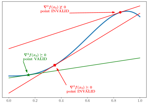
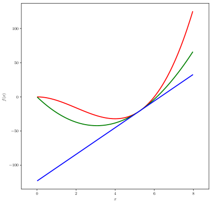
We also note that the validity of the bound on overestimation computed by (4) is predicated on the premise that is convex, and if the selection of nullifies this premise, then the bound yielded by (4) is no longer valid. We highlight that the condition ) is not sufficient in the non-convex case, as a first-order Taylor series approximation constructed at a point (even where ) is not guaranteed to underestimate a non-convex function over the entire domain. Figure 1 illustrates this concept with a non-convex d.c. function and three first-order Taylor series approximations, created at three candidate points of construction that each demonstrates different possibilities: (i) a point where , for which the tangent line does not even underestimate locally, (ii) a point where , for which the tangent line underestimates locally but not throughout the whole domain, and (iii) a point where for which the tangent line constitutes a valid underestimator. Obviously, it is only in the last case that one can construct a valid quadratic underestimator of the form of (1).
2.4 Generalization to a Hierarchy of Quadratic Underestimators
Considering the fact that the scalar uniformly scales the elements of in (1), we generalize the quadratic form and present a hierarchy of quadratic underestimators that allows for the construction of tighter underestimators. Before presenting the methodology for each underestimator, we restate key ideas and relevant algorithmic steps for understanding and implementing our hierarchy. In the remainder of the manuscript, we use to indicate a point at which , where is a user-specified tolerance and superscript “” denotes the value of the scaling variable at iteration of the cutting plane algorithm.
Corrective action is taken in Step 5 of the cutting plane algorithm to suitably recompute the parameter of the quadratic. Here, we restate Step 5 as well as Observation 1 from Strahl et al. [2024], which elucidates a key property for our quadratic underestimators, i.e., that the quadratic monotonically decreases with respect to a decrease in , which can be exploited to improve algorithmic efficiency.
Step 5. Evaluate Underestimation:
,
where is the set of new vertices enumerated with the introduction of a cutting plane.
Observation 1 (for proof, see Strahl et al. [2024]).
The quadratic underestimator in (1) monotonically decreases as decreases; that is, for all .
The goal of the following presentation is to generalize the quadratic underestimator form to allow the construction of tighter underestimators, while preserving the efficiency of the algorithm by enforcing the quadratic to monotonically nonincrease each time the parameters are updated. We note that changes at are the same, regardless of whether the function is convex or d.c., and will therefore hereafter reference the function to be underestimated as , which in the d.c. case can be substituted directly with . We begin our presentation with the original method developed in Strahl et al. [2024], which for purposes of the hierarchy, we shall refer to as the “scalar” method.
2.4.1 Scalar Method
2.4.2 Diagonal Method
We generalize the quadratic form in method “S” by introducing a diagonal matrix of scaling parameters, , into the eigenvalue decomposition of , , as shown in (5), which permits the scaling parameters, i.e., the diagonal elements of , to modify each eigenvalue of differently, while the off-diagonal elements are fixed to 0. Hence, we refer to this method as the “diagonal” method, or method “D”.
| (5) |
The new quadratic form (5) requires a different procedure for determining the scaling parameters, such that each new selection: (i) ensures the quadratic underestimates the function at ; (ii) monotonically decreases the quadratic over the entire domain with each consecutive update to the parameters; and (iii) produces the tightest possible quadratic underestimator over the entire domain, when the algorithm converges. Observing that the (diagonal) elements of participate linearly in the quadratic form, we can compute them via the linear program (D), where we explicitly enforce (i) and (ii) in the constraints.
| (D) |
where is the incumbent value for the diagonal elements of the scaling matrix (to be updated with the optimal solution of this LP).
To accomplish (iii), the above LP aims to explicitly optimize for “tightness” or quality of the produced underestimator. For this, we utilize the metric (6), defined in Strahl et al. [2024], that quantifies the tightness of the quadratic underestimator, , as the fractional reduction in hypervolume from a function to it, when compared to a linear underestimator, , generated at the same point of construction.
| (6) |
As we consider utilizing this metric as the objective in the LPs for our methods, we make the following observation, where is a set of points .
Observation 2.
In the case that , the constraint for all , in conjunction with the objective , produces the tightest scaling parameters by construction, thereby achieving objective (iii).
Since sampling an infinite amount of points at which to evaluate underestimating distances is not practical, we discretize the space by choosing points, where is the dimension of the problem and the points are selected via a Latin hypercube approach. To embed the metric directly in the LP, we remove constant terms from (6) to produce the objective function in (D), which maximizes the value of the quadratic at each sampled point. However, the constraints in (D) only enforce underestimation at a single point, namely . This fact, considered together with the monotonicity requirement imposed on the parameters, results in the algorithm making greedy initial commitments to parameter values which, although optimal in light of , may ultimately yield sub-optimal parameter values at termination.
To address this behavior, we recommend augmenting the formulation of the first LP we ever solve with the constraints for all , resulting in formulation (), which provides an update to the parameters using a holistic treatment of the space. These additional constraints are only required for the first LP executed in the cutting plane algorithm; subsequent LPs can be relaxed to contain only the single constraint (formulation D), since monotonicity guarantees underestimation for these points through the remaining execution of the algorithm. We highlight that an interesting tradeoff arises between the number of points in set and the number of LPs that have to be solved throughout the algorithm. Despite yielding a larger LP (), which however need only be solved once at the first iteration, larger typically leads to detecting fewer points of overestimation, creating tighter underestimators while requiring fewer LPs (D) to be solved in the long run.
| () |
where we initialize for all rows .
We remark the following regarding the diagonal scaling method: (i) () has constraints in the first iteration, after which (D) has constraints; thus, these LPs are small in size; (ii) we know that the value of is a valid upper bound on each element of the diagonal of , , because the quadratic would overestimate locally at the point of construction if any ; and (iii) “S” can be viewed as a restriction of method “D”, where additional constraints are added in (D) to achieve equivalency for all ; indeed, the final parameter determined by method “S” used for all the diagonal elements of will be feasible to (D), but due to the inexactness introduced from sampling the space (finite set ), formulation (D) can possibly produce an inferior underestimator, the mitigation of which is encouraged by ().
2.4.3 Matrix Method
We further generalize the diagonal scaling method to allow modifications to the off-diagonal elements of as well, where the quadratic underestimator form is the same as (5), but we remove the restriction that the off-diagonal elements of must be . We shall refer to this method as the “matrix” method, or method “M”.
While the quadratic form does not change from the diagonal scaling method, the introduction of off-diagonal variables in necessitates a more involved LP to preserve the required properties of the quadratic. First and foremost, we are interested in producing convex quadratic underestimators, for which we had trivial guarantees in previous methods, as we directly scaled eigenvalues with . However, modifying the off-diagonal elements gives rise to the possibility of creating non-convex quadratics even with non-negative diagonal elements. To that end, we explicitly enforce convexity during each parameter update by requiring to be diagonally dominant, which is a sufficient condition for the positive semi-definiteness of . To invoke this property, we first require symmetry on and non-negativity of all diagonal elements , which ensures that due to at the selected point of construction. Then, we impose the diagonal dominance property by requiring that for all rows .
Lastly, to preserve the algorithmic efficiency of the cutting plane algorithm achieved by exploiting the monotonicity property of the quadratic (Observation 1), we utilize the fact that implies that for all , where are the incumbent values of the parameters at the time the LP is executed. This realizes the desired monotonicity property, since the orthogonality of in the eigenvalue decomposition preserves the eigenvalues of . For the constraint requiring , we similarly impose the diagonal dominance property on matrices . Based on the above, the computation of can be achieved via formulation (M), which can be trivially reformulated to the LP in (M′) after the introduction of auxiliary variables and .
| (M) |
| (M′) |
We highlight that the LP (M′) has variables and constraints. Despite being a more involved LP than the one encountered in the diagonal method, it is still expected to be very tractable in practice.
2.4.4 Shift
In Section 2.3, we established a necessary–but not sufficient–condition for the selection of point of construction to yield a valid quadratic underestimator generated by our cutting plane algorithm. Here, we introduce a term into the quadratic forms (1) and (5) to allow for their vertical (downward) shift. We show how to properly update (S), (D) (or ) and (M′) to accommodate the augmented form, and how the introduction of the shift causes the necessary condition to also become sufficient for our methodology to produce valid quadratic underestimators. For all methods, we denote the scalar variable for the shift as , which is initialized to , and which is to be negated from the applicable quadratic form (1) or (5) in each case. To differentiate from the previous methods without shift, we augment the label of our methods that include the shift with the letter “S” (e.g., “DS” refers to the diagonal method with shift).
For the scalar method, we utilize a shift only if method “S” computes , whereupon we reset and update throughout each iteration using (SS). While computationally inexpensive, this approach (dubbed method “SS”) will effectively produce a linear underestimator when the shift is indeed required (i.e., a vertical shift of the first-order Taylor series approximation).
| (SS) |
Before we present the incorporation of shift in the methods utilizing a scaling matrix in lieu of a scalar , we consider a hybrid method that requires identical elements in a diagonal matrix. Consistent with the rest of the hierarchy, we will refer to this as method as “UDS” (i.e., “uniform diagonal with shift”). In this method, both scalar parameters (the common element in the diagonal) and can be optimized simultaneously via the LP (UDS). We also highlight the inclusion of the constraint , which imposes the monotonicity property of the quadratic from iteration to iteration. Importantly, this enforcement of monotonicity preserves the requisite properties for the cutting plane algorithm’s convergence proof [Strahl et al., 2024] after the addition of the shift. We also remark that method “UDS” is a generalization of both methods “SS” and “S” inasmuch as any results determined by the latter two are also feasible to “UDS”, noting however that the relative tightness of these underestimators might be affected by the selection of the set .
| (UDS) |
where is the incumbent value for the shift variable (to be updated with the optimal solution of this LP).
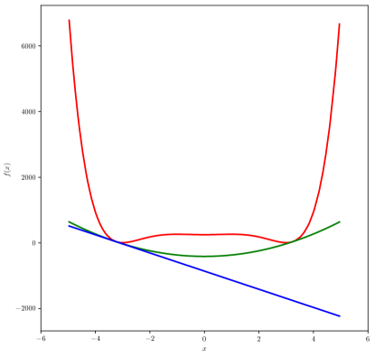
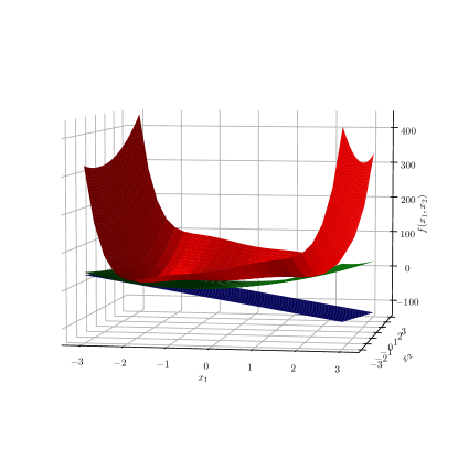
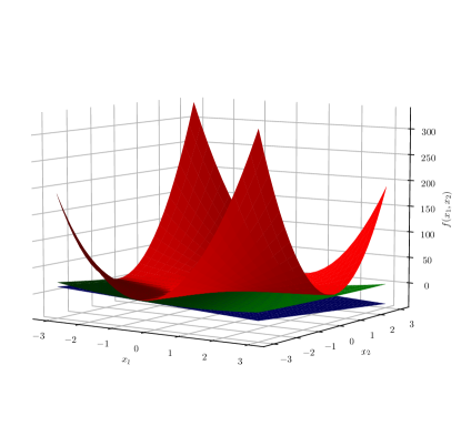
In summary, in the hierarchy of using a mere scalar in the quadratic form, we have: (i) method “S”, which may fail to produce a valid underestimator for certain points of construction in the case of non-convex d.c. functions; (ii) method “SS”, which is efficient to compute but will only produce a linear underestimator, and should hence be reserved only for the points of construction where “S” fails; and (iii) method “UDS”, which requires solving LPs but will produce a valid underestimator for all points of construction where (at worst a linear underestimator, but likely a quadratic one). Figure 2 demonstrates an example where utilizing method “UDS” constructs a successful quadratic underestimator when method “S” would otherwise fail due to poor choice of the point of construction. Finally, we highlight that, in certain instances, a combination of and in method “UDS” could achieve even tighter underestimators, as measured by relative hypervolumes; however, for our computational studies, we keep the upper bound of parameter at and initialize .
We now turn our attention to the incorporation of shift in the methods utilizing scaling matrices, introducing methods “DS” and “MS”. For this, the linear programs defined by (D) and (M′) are updated analogously to (UDS), where we incorporate the variable and impose the constraint to preserve monotonicity. This results in linear programs (DS) and (MS), respectively for the two methods.
| (DS) |
| (MS) |
Overall, we have presented a hierarchy of methods that can produce quadratic underestimators of non-convex d.c. functions at user-specified points of construction. This hierarchy is presented in a diagram in Figure 3, where tighter–but more computationally expensive–underestimators lie at the bottom and to the right. We remind readers that all the methods not in blue require solving an LP to update their parameters. Finally, we emphasize the fact that all quadratic forms and update procedures are immediately amenable to, without further modification, the methodological extension presented in Strahl et al. [2024], where information of external linear constraints in optimization problems can be exploited to produce tighter underestimators by allowing them to overestimate in infeasible regions.
3 Computational Study
We demonstrate the performance of our hierarchy of quadratic underestimators generated by our cutting plane algorithm for non-convex d.c. functions in two distinct computational experiments. In the first experiment in Section 3.1, we extract d.c. functions from optimization problems found in benchmark libraries and we construct underestimators for them, showcasing their efficiency and tightness. In the second experiment in Section 3.2, we compare the root node relaxation of the state-of-the-art global optimization solver BARON with a convex quadratic relaxation constructed via our methodology on optimization problems with d.c objectives and constraints.
3.1 Hierarchy Comparison Study
For our study on the tightness and computational efficiency of our hierarchy of underestimators, we extracted 3 one-dimensional and 7 two-dimensional d.c. functions from the COCONUT library (https://arnold-neumaier.at/glopt/coconut/Benchmark/Benchmark.html), which compiles optimization problems from GlobalLib, CUTE, and Constraint satisfaction test problems (CSTP) libraries. The location of the problems in the COCONUT library and the explicit expressions used in the computational study are included in Table A1 in the Appendix. We note that we employed the relationships and to create d.c. representations for many of the functions found in the optimization libraries. Where necessary, we assigned bounds to otherwise unbounded variables as noted in Table A1, and we scaled the range of the functions to lie within the interval by using the scaling factor . For each function, we used Latin hypercube sampling of its domain until we could accumulate 25 points of construction where the function is locally convex, as assessed via eigenvalue decomposition of the Hessian at those points. Finally, we used the value e for the convergence tolerance of the cutting plane algorithm. Our computational experiments were executed on a machine equipped with a 1.80GHz Intel(R) Core(TM) i7-8565U CPU running on a Ubuntu 22.04 virtual machine with 8GB RAM and 4 logical processors, where we have implemented the algorithms in Python. To solve LPs, we used the open source HiGHS [Huangfu and Hall, 2018] linear program solver, which is included in the Python SciPy package [Virtanen et al., 2020], and which was found to be adequate to address the small sized LPs encountered in this study.
3.1.1 Results
Qualitatively, Figure 4 depicts the underestimators created by the methods “S”, “D” and “M” for a function from the dipigri optimization problem, highlighting the possible improvement in underestimator tightness by using ever more sophisticated techniques. Additionally, Figures 5 and 6 visualize some examples of our quadratic underestimators constructed for non-convex d.c. functions, as generated by the “S” method.

Performing a quantitative comparison among the methods in the hierarchy requires categorizing the functions along with points of construction into two groups: (i) those for which methods that do not utilize shift can construct a successful quadratic underestimator, where the entire hierarchy can be compared; and (ii) those for which construction procedures require the shift for success (i.e., first-order Taylor series approximations do not underestimate across the full domain of interest), and hence, where only the methods “SS”, “UDS”, “DS” and “MS” can be compared. Accordingly, Tables 1 and 2 display the average tightness metric, computed via (6), and the CPU time (in milliseconds) required to compute the underestimators for groups (i) and (ii), respectively.
| Dimension | # Functions | # Points of Construction | Avg. Metric | Avg. CPU (ms) | ||||||||||||
| S | D | M | SS | UDS | DS | MS | S | D | M | SS | UDS | DS | MS | |||
| 1 | 3 | 36 | 0.559 | 0.559 | 0.559 | 0.559 | 0.559 | 0.559 | 0.559 | 4 | 11 | 13 | 6 | 11 | 11 | 14 |
| 2 | 7 | 90 | 0.384 | 0.449 | 0.464 | 0.384 | 0.467 | 0.499 | 0.502 | 35 | 93 | 125 | 44 | 98 | 114 | 133 |
Dimension # Functions # Points of Construction Avg. Metric Avg. CPU (ms) SS UDS DS MS SS UDS DS MS 1 3 39 0.000 0.014 0.014 0.014 4 9 8 12 2 7 85 0.000 0.094 0.115 0.122 34 75 73 96
For functions of one dimension, Table 1 clearly shows that all methods perform similarly for points of construction that admit valid underestimators without requiring a shift, which is simply explained by the equivalency of the methods in the univariate case. In the case of bivariate functions, however, Table 1 shows that the shift provides some flexibility to create tighter underestimators. This is evidenced by the sharp increase of 0.083 (21.6%) in the average metric between methods “S” and “UDS”, as compared to the less significant improvement of 0.065 (16.9%) between “S” and “D”. Using the matrix methods in lieu of the diagonal ones yields only marginal improvements in underestimator tightness, as indicated by the increase of 0.015 (3.3%) and 0.003 (0.6%) in the average metric, respectively for the unshifted (“D” vs. “M”) and shifted (“DS” vs. “MS”) methods. As expected, method “MS” constructs the tightest underestimators, but it also exacts the greatest computational expense.
Table 2 demonstrates the effectiveness of the shift and the capability for the methodologies to construct quadratic underestimators at points where, without the shift, the methods would fail. First, we clearly state that all methods with the shift successfully create underestimators for all points of construction, without exception. However, given that the first-order Taylor series approximation constructed at these points is not a valid underestimator, we ought to use an altered definition of the metric to convey tightness. More specifically, in Table 2, the reported metric compares the linear underestimator generated by method “SS” with underestimators constructed by the other methods; hence, method “SS” is reported in Table 2 as having a metric of , by definition. Notably, the other methods show a metric greater than , indicating that the final underestimators generated by these methods retain some curvature. Indeed, for the bivariate case, we observe that simultaneously optimizing the parameter(s) with the shift produces underestimators that reduce the volume between the function and the linear underestimators generated by “SS” by 9.4%, 11.5%, and 12.2%, respectively for methods “UDS”, “DS” and “MS”. These results demonstrate the importance of using the shift parameter to successfully achieve quadratic underestimation at any and all points of construction for which and to improve the tightness of these underestimators.
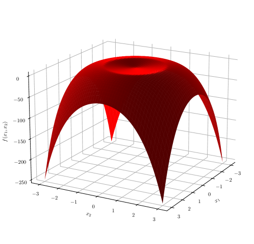
Tables A2 and A3 in the Appendix provide detailed data for each method regarding the average and standard deviation of cutting plane algorithm iterations, number of vertices enumerated, metric, CPU time, and number of LP solves for the computational study. Finally, we remark that, in our extraction of d.c. functions, certain pathological cases (e.g., a function from the sisser optimization problem showed in Figure A1 in the Appendix were identified but not removed from our benchmark set. In these cases, pathological refers to functions for which the cutting algorithm will fail to generate a successful quadratic underestimator at all points without the shift.
3.2 Root Node Relaxation Comparison with State-of-the-art
In this study, we demonstrate the quality of relaxations constructed using our quadratic underestimation methodology on a set of d.c. optimization problems. In particular, we employ method “DS”, which affords a good tradeoff between quality and tractability, to construct quadratic underestimators for each non-linear function in these problems, setting the tolerance of the cutting plane algorithm to e. We then solve the resulting convex QCQP relaxation using IPOPT v3.14.13 [Wächter and Biegler, 2006] with the linear solver MUMPS v5.6.2 [Amestoy et al., 2001, 2006] to determine a lower bound at the root node of each problem, which we compare with the lower bound at the root node computed by BARON v24.5.8 [Sahinidis, 1996]. We use all default settings of BARON, including the option NoutPerVar = 4 that dictates the number of outer approximations per variable for convex multivariate functions. For a fair comparison, we mirror this by choosing to construct four quadratic underestimators per dimension at points of construction determined using Latin hypercube sampling, for each non-linear function present in the benchmark problems. Aside from this, we use the same settings for the cutting plane algorithm, as presented in Section 3.1. We also highlight that we include all auxiliary techniques available by default in BARON (e.g., bounds tightening), even though equivalent techniques are not utilized in our methodology. Despite such an unfavorable setup, however, we will demonstrate the superior quality of the lower bounds computed using our convex quadratic relaxation for problems defined in dimensions greater than one.
3.2.1 Generation of D.C. Optimization Problem Library
Noting the scarcity of benchmark d.c. optimization problems available in the literature, we systematically created optimization problems that are defined in one to four dimensions and that include linear, convex, and (non-convex) d.c. functions. Whereas the explicit problem instances used in our computational study are provided in the Appendix, in this section we outline the general procedure we employed in creating these instances.
We generate optimization problems parameterized by a tuple, , where is the dimension of the problem, is the number of linear constraints, is the number of convex constraints, and is the number of non-convex d.c. constraints. For our study, we produce instances defined using all combinations of , if (no linear constraints added in univariate optimization problems), and . In total, we produce 24 problems (6 for each dimension). In all cases, we restrict the domain of the variables to .
To create a new instance, we first assign to the desired dimension, and then select a d.c. function to serve as the objective, followed by , , and linear, convex, and d.c. functions, respectively, to serve as constraints. As we add a new constraint to the problem, we ensure it is not redundant (i.e., it does reduce the feasible space) by utilizing a set of points selected via Latin hypercube sampling to check for feasibility. More specifically, given the domain of the variables, , we determine a priori the upper and lower bounds of the range of each function, where the upper bound defines a right-hand side for the constraint to encompass the full feasible space (i.e., makes the constraint redundant), and the lower bound defines a right-hand side that eliminates the entire feasible space (i.e., causes the problem to be infeasible). Via binary search, we pick the right-hand side to use for this constraint such that % of the remaining sampled feasible points are eliminated. For example, after we sample 400 points for a four dimensional problem, the first constraint added will eliminate 80 of those from the feasible space, while the next constraint will eliminate an additional 64 (% of the remaining 320) points, resulting in 256 feasible points in the original sample.
Consequently, the order in which the constraints are added to the optimization problem is important: we add the linear constraint first, followed by the convex constraints, and add the d.c. constraints last. We highlight that adding the constraints in this order maximizes the contribution of the non-convex d.c. functions in defining the feasible space, which aligns with the goal of this work.
We generate linear constraints for use in our optimization problems by considering the linear form , where or (chosen randomly) for each dimension . As per the process explained above, we identify bounds on range of each linear expression and execute a binary search on until the feasible space (as represented by the sample points) has been reduced by %. In regards to generating convex functions, we do so by randomly sampling from a core set of convex functional forms extracted from benchmark libraries and expanded using established rules that preserve convexity. To create d.c. functions, we take special care to ensure the functions are non-convex and multi-modal over the prescribed domain. We begin with a core set of six univariate non-convex d.c. functions (see Table A4 in the Appendix), which we add up to construct higher dimensional d.c. functions while also adding a “linking term”, , where is the number variables included in a particular multi-dimensional d.c. function. The linking term induces inseparable variable dependencies on the function output, which prevents trivially separating terms that could otherwise have been underestimated separately. After randomly shuffling all possible combinations of higher dimensional d.c. functions utilizing the core set of six, we use the first d.c. function in the objective, and subsequent functions in the d.c. constraints until we have added a total of constraints.
While we omit many specific details from our problem construction description, we include the explicit problems in Tables A5–A8 in the Appendix for reference. We note that these tables only present floating point numbers to three decimals of precision; consequently, we supply the .nl files defining the problems with full decimal precision as executed in this study as Supplementary Material to this paper. We additionally provide a comprehensive list of the points of construction for each function of the study, included as comments in each file.
3.2.2 Results
Table 3 provides aggregate results for the root node relaxation comparison, where we report the number of instances for which each alternative approach–QCQP relaxation versus BARON–computes a superior root node lower bound as well as the average reduction of the gap between the optimal solution and the BARON lower bound that the QCQP relaxation affords us. These results demonstrate that the convex QCQP relaxation produces substantially superior lower bounds compared to BARON, reducing the root node relaxation gap by an excess of 92%, on average, for problems defined in two or more dimensions. For univariate problems, the QCQP relaxation produces tighter lower bounds than BARON at the root node for five out of the six problem instances, while for the sixth problem, BARON reduced the gap between the QCQP bound and the optimal solution by only 11%. These results provide strong evidence of the tightness of the convex QCQP relaxation constructed by our methodology. We acknowledge that, while this comparison provides evidence for the quality of the quadratic underestimators generated by our methodology, the latter requires more computation time than BARON. However, given that we have implemented our algorithms in Python, it remains to be seen whether efficiency gains that would be achieved by utilizing a compiled language can provide for a more straightforward comparison.
Dimension # Problems BARON Root Node Better QCQP Bound Better Avg. Gap Reduction by QCQP 1D 6 1 5 78.8%∗ 2D 6 0 6 92.1% 3D 6 0 6 94.4% 4D 6 0 6 94.5% ∗Reduction for the 5 problems where the QCQP provided a better bound.
4 Conclusions
In this work, we presented a hierarchy of methodologies to construct convex quadratic underestimators for non-convex d.c. functions. Focusing on d.c. functions extracted from optimization benchmark libraries, we generated quadratic underestimators that reduce the hypervolume between the function and a linear underestimator constructed at the same point of construction by 55.9% for one-dimensional functions and, depending on the variant of our methodology used, by a range of 38.4%-50.2% for two-dimensional functions, on average. Furthermore, we demonstrated in our computational study that, with variants that include a shift in the quadratic form, we could generate valid underestimators for all points of construction where , including points at which the first-order Taylor series approximation is not a valid underestimator. We showcase the tightness of our quadratic underestimators by providing qualitative results on several example functions, highlighting also the improvements that can be achieved by utilizing more involved methods in our hierarchy. Finally, we show the quality of convex QCQP relaxations constructed using our quadratic underestimation methodology in a comparison with BARON for lower bounds computed at the root node of a set of systematically created d.c. optimization problems. Notably, our convex QCQP relaxation is able to produce superior lower bound than those computed by BARON at the root node in the vast majority of cases, closing the root node relaxation gap by 90%, on average.
Future work could investigate generalizing the hierarchy even further to include variants that determine a matrix for the second-order term of the Taylor series approximation from the entire positive semi-definite cone, rather than from a restricted subset limited to matrices satisfying diagonal dominance properties. In our experience, maintaining a quadratic that is monotonic in its parameters is much more involved with a parameter modifying the first-order term of the quadratic. Thus, future work could explore ways to tailor the cutting plane algorithm to achieve the monotonicity property in the context of modifying the first-order term, or altogether removing the monotonicity requirement from the algorithm while preserving efficiency and convergence.
Acknowledgments
We acknowledge financial support from Mitsubishi Electric Research Labs (MERL) through the Center for Advanced Process Decision-making (CAPD) at Carnegie Mellon University. William Strahl also gratefully acknowledges support from the R.R. Rothfus Graduate Fellowship in Chemical Engineering and the Chevron Graduate Fellowship in Chemical Engineering.
Appendix
The material supplied in this appendix provides the explicit function and problem formulations used in our computational study as well as supplemental details for some of the results. More specifically, Table A1 displays the precise functions used in Section 3.1.1, while Tables A2 and A3 provide additional details for the computational results of the same section.
Figure A1 provides a visual example of a pathological function discovered in the study for quadratic underestimator forms without the shift parameter. Finally, for the computational study in Section 3.2, where we compare root node relaxations of optimization problems, Tables A4–A8 provide all the required information to construct the problems used in the study. All models are supplied in the Supplementary Material accompanying this paper in the form of .nl files, which also include the points used as points of construction for the computational results in Section 3.2.2.
Dimension Library Problem Name Expression Variable Bounds Assigned Bounds 1 GlobalLib ex4_1_6 objcons (-5, 5) – 1 CUTE zy2 objcons (0, 8) Upper 1 GlobalLib ex4_1_9 con1 (0, 3) – 2 CSTP conform1 con2, (-3, 3), (-3, 3) Both 2 GlobalLib ex8_1_4 objcons (-3, 3), (-3, 3) Both 2 CUTE camel6 objcons (-3, 3), (-1.5, 1.5) – 2 CUTE sisser objcons (-3, 3), (-3, 3) Both 2 CSTP cyclo con1 (-10, 10), (-10, 10) – 2 GlobalLib ex4_1_5 objcons (-5, 5), (-5, 5) Upper for and lower for 2 CUTE dipigri objcons (-3, 3), (-3, 3) Both
| Method | Iterations | Vertices | Metric | CPU (ms) | LP Solves |
| S | |||||
| D | |||||
| M | |||||
| SS | |||||
| UDS | |||||
| DS | |||||
| MS |
| Method | Iterations | Vertices | Metric | CPU (ms) | LP Solves |
| SS | |||||
| UDS | |||||
| DS | |||||
| MS |
| Functions |
Problem # Definition 01 02 03 04 05 06
Problem # Definition 07 08 09 10 11 12
Problem # Definition 13 14 15 16 17 18
Problem # Definition 19 20 21 22 23 24
References
- Adjiman et al. [1998a] Claire S Adjiman, Ioannis P Androulakis, and Christodoulos A Floudas. A global optimization method, BB, for general twice-differentiable constrained NLPs—II. Implementation and computational results. Computers & chemical engineering, 22(9):1159–1179, 1998a.
- Adjiman et al. [1998b] Claire S Adjiman, Stefan Dallwig, Christodoulos A Floudas, and Arnold Neumaier. A global optimization method, BB, for general twice-differentiable constrained NLPs—I. Theoretical advances. Computers & Chemical Engineering, 22(9):1137–1158, 1998b.
- Akrotirianakis et al. [2004] IG Akrotirianakis, CA Meyer, and CA Floudas. The role of the off-diagonal elements of the hessian matrix in the construction of tight convex underestimators for nonconvex functions. Discovery Through Product and Process Design, pages 501–504, 2004.
- Alvarado et al. [2014] Alberth Alvarado, Gesualdo Scutari, and Jong-Shi Pang. A new decomposition method for multiuser dc-programming and its applications. IEEE Transactions on Signal Processing, 62(11):2984–2998, 2014.
- Amestoy et al. [2001] P. R. Amestoy, I. S. Duff, J. Koster, and J.-Y. L’Excellent. A fully asynchronous multifrontal solver using distributed dynamic scheduling. SIAM Journal on Matrix Analysis and Applications, 23(1):15–41, 2001.
- Amestoy et al. [2006] P. R. Amestoy, A. Guermouche, J.-Y. L’Excellent, and S. Pralet. Hybrid scheduling for the parallel solution of linear systems. Parallel Computing, 32(2):136–156, 2006.
- Androulakis et al. [1995] Ioannis P Androulakis, Costas D Maranas, and Christodoulos A Floudas. BB: A global optimization method for general constrained nonconvex problems. Journal of Global Optimization, 7:337–363, 1995.
- Askarizadeh et al. [2023] Mohammad Askarizadeh, Alireza Morsali, Mostafa Zangiabadi, and Kim Khoa Nguyen. Difference convex (dc) programming approach as an alternative optimizer for neural networks. In ICC 2023-IEEE International Conference on Communications, pages 5179–5184. IEEE, 2023.
- Awasthi et al. [2024] Pranjal Awasthi, Anqi Mao, Mehryar Mohri, and Yutao Zhong. DC-programming for neural network optimizations. Journal of Global Optimization, pages 1–17, 2024.
- Bagirov and Ugon [2018] Adil M Bagirov and Julien Ugon. Nonsmooth DC programming approach to clusterwise linear regression: optimality conditions and algorithms. Optimization methods and software, 33(1):194–219, 2018.
- Bagirov et al. [2016] Adil M Bagirov, Sona Taheri, and Julien Ugon. Nonsmooth DC programming approach to the minimum sum-of-squares clustering problems. Pattern Recognition, 53:12–24, 2016.
- Bertsekas et al. [2003] Dimitri Bertsekas, Angelia Nedic, and Asuman Ozdaglar. Convex analysis and optimization, volume 1. Athena Scientific, 2003.
- Bertsimas et al. [2023] Dimitris Bertsimas, Danique de Moor, Dick den Hertog, Thodoris Koukouvinos, and Jianzhe Zhen. A novel algorithm for a broad class of nonconvex optimization problems. Optimization Online, 2023.
- Boukouvala et al. [2016] Fani Boukouvala, Ruth Misener, and Christodoulos A Floudas. Global optimization advances in mixed-integer nonlinear programming, MINLP, and constrained derivative-free optimization, CDFO. European Journal of Operational Research, 252(3):701–727, 2016.
- Buchheim and Trieu [2013] Christoph Buchheim and Long Trieu. Quadratic outer approximation for convex integer programming with box constraints. In Experimental Algorithms: 12th International Symposium, SEA 2013, Rome, Italy, June 5-7, 2013. Proceedings 12, pages 224–235. Springer, 2013.
- Chen et al. [1998] Pey-Chun Chen, Pierre Hansen, Brigitte Jaumard, and Hoang Tuy. Solution of the multisource Weber and conditional weber problems by d.-c. programming. Operations Research, 46(4):548–562, 1998.
- Durkin et al. [2024] Alex Durkin, Lennart Otte, and Miao Guo. Surrogate-based optimisation of process systems to recover resources from wastewater. Computers & Chemical Engineering, page 108584, 2024.
- Gasso et al. [2009] Gilles Gasso, Alain Rakotomamonjy, and Stéphane Canu. Recovering sparse signals with a certain family of nonconvex penalties and DC programming. IEEE Transactions on Signal Processing, 57(12):4686–4698, 2009.
- Gounaris and Floudas [2008a] Chrysanthos E Gounaris and Christodoulos A Floudas. Tight convex underestimators for-continuous problems: I. Univariate functions. Journal of Global Optimization, 42(1):51–67, 2008a.
- Gounaris and Floudas [2008b] Chrysanthos E Gounaris and Christodoulos A Floudas. Tight convex underestimators for-continuous problems: II. Multivariate functions. Journal of Global Optimization, 42(1):69–89, 2008b.
- Hartman [1959] Philip Hartman. On functions representable as a difference of convex functions. 1959.
- Hoffman [1981] Karla Leigh Hoffman. A method for globally minimizing concave functions over convex sets. mathematical Programming, 20:22–32, 1981.
- Holmberg and Tuy [1999] Kaj Holmberg and Hoang Tuy. A production-transportation problem with stochastic demand and concave production costs. Mathematical programming, 85:157–179, 1999.
- Horst and Pardalos [2013] Reiner Horst and Panos M Pardalos. Handbook of global optimization, volume 2. Springer Science & Business Media, 2013.
- Huangfu and Hall [2018] Qi Huangfu and JA Julian Hall. Parallelizing the dual revised simplex method. Mathematical Programming Computation, 10(1):119–142, 2018.
- Kim et al. [2022] Minsu Kim, Sunghyun Cho, Kyojin Jang, Seokyoung Hong, Jonggeol Na, and Il Moon. Data-driven robust optimization for minimum nitrogen oxide emission under process uncertainty. Chemical Engineering Journal, 428:130971, 2022.
- Le Thi and Nguyen [2017] Hoai An Le Thi and Manh Cuong Nguyen. DCA based algorithms for feature selection in multi-class support vector machine. Annals of Operations Research, 249(1-2):273–300, 2017.
- Lou et al. [2015] Yifei Lou, Tieyong Zeng, Stanley Osher, and Jack Xin. A weighted difference of anisotropic and isotropic total variation model for image processing. SIAM Journal on Imaging Sciences, 8(3):1798–1823, 2015.
- Lu et al. [2023] Yen-An Lu, Conor M O’ Brien, Douglas G Mashek, Wei-Shou Hu, and Qi Zhang. Kinetic-model-based pathway optimization with application to reverse glycolysis in mammalian cells. Biotechnology and bioengineering, 120(1):216–229, 2023.
- Maranas and Floudas [1995] Costas D Maranas and Christodoulos A Floudas. Finding all solutions of nonlinearly constrained systems of equations. Journal of Global Optimization, 7:143–182, 1995.
- McCormick [1976] Garth P McCormick. Computability of global solutions to factorable nonconvex programs: Part I—convex underestimating problems. Mathematical programming, 10(1):147–175, 1976.
- Melzer [1986] D Melzer. On the expressibility of piecewise-linear continuous functions as the difference of two piecewise-linear convex functions. Quasidifferential Calculus, pages 118–134, 1986.
- Meyer and Floudas [2005] Clifford A Meyer and Christodoulos A Floudas. Convex underestimation of twice continuously differentiable functions by piecewise quadratic perturbation: Spline BB underestimators. Journal of Global Optimization, 32:221–258, 2005.
- Mitsos et al. [2009] Alexander Mitsos, Benoit Chachuat, and Paul I Barton. McCormick-based relaxations of algorithms. SIAM Journal on Optimization, 20(2):573–601, 2009.
- Mittelmann [2023] Hans Mittelmann. Benchmarks for optimization software, 2023. URL https://plato.asu.edu/bench.html. Accessed on December 23, 2023.
- Nguyen and Le Thi [2023] Phuong Anh Nguyen and Hoai An Le Thi. DCA approaches for simultaneous wireless information power transfer in MISO secrecy channel. Optimization and Engineering, 24(1):5–29, 2023.
- Olama et al. [2023] Alireza Olama, Eduardo Camponogara, and Paulo RC Mendes. Distributed primal outer approximation algorithm for sparse convex programming with separable structures. Journal of Global Optimization, 86(3):637–670, 2023.
- Ouanes et al. [2015] Mohand Ouanes, Hoai An Le Thi, Trong Phuc Nguyen, and Ahmed Zidna. New quadratic lower bound for multivariate functions in global optimization. Mathematics and Computers in Simulation, 109:197–211, 2015.
- Öztürk and Köksalan [2023] Diclehan Tezcaner Öztürk and Murat Köksalan. Biobjective route planning of an unmanned air vehicle in continuous space. Transportation Research Part B: Methodological, 168:151–169, 2023.
- Sahinidis [1996] Nikolaos V Sahinidis. BARON: A general purpose global optimization software package. Journal of global optimization, 8:201–205, 1996.
- Sherali and Adams [2013] Hanif D Sherali and Warren P Adams. A reformulation-linearization technique for solving discrete and continuous nonconvex problems, volume 31. Springer Science & Business Media, 2013.
- Skjäl et al. [2012] Anders Skjäl, Tapio Westerlund, Ruth Misener, and Christodoulos A Floudas. A generalization of the classical BB convex underestimation via diagonal and nondiagonal quadratic terms. Journal of Optimization Theory and Applications, 154:462–490, 2012.
- Strahl et al. [2024] William R. Strahl, Arvind Raghunathan, Nikolaos V. Sahinidis, and Chrysanthos E. Gounaris. Constructing tight quadratic relaxations for global optimization: I. Outer-approximating twice-differentiable convex functions. Forthcoming, 2024.
- Streeter and Dillon [2022] Matthew Streeter and Joshua V Dillon. Automatically bounding the Taylor remainder series: Tighter bounds and new applications. arXiv preprint arXiv:2212.11429, 2022.
- Streeter and Dillon [2023] Matthew Streeter and Joshua V Dillon. Sharp taylor polynomial enclosures in one dimension. arXiv preprint arXiv:2308.00679, 2023.
- Su et al. [2018] Lijie Su, Lixin Tang, David E Bernal, and Ignacio E Grossmann. Improved quadratic cuts for convex mixed-integer nonlinear programs. Computers & Chemical Engineering, 109:77–95, 2018.
- Tsoukalas and Mitsos [2014] Angelos Tsoukalas and Alexander Mitsos. Multivariate mcCormick relaxations. Journal of Global Optimization, 59(2-3):633–662, 2014.
- Virtanen et al. [2020] Pauli Virtanen, Ralf Gommers, Travis E Oliphant, Matt Haberland, Tyler Reddy, David Cournapeau, Evgeni Burovski, Pearu Peterson, Warren Weckesser, Jonathan Bright, et al. SciPy 1.0: Fundamental algorithms for scientific computing in Python. Nature methods, 17(3):261–272, 2020.
- Wächter and Biegler [2006] Andreas Wächter and Lorenz T Biegler. On the implementation of an interior-point filter line-search algorithm for large-scale nonlinear programming. Mathematical programming, 106:25–57, 2006.
- Yang et al. [2022] Yu Yang, Brenda De La Torre, Katherine Stewart, Laurianne Lair, Nguyen L Phan, Rupak Das, Demar Gonzalez, and Roger C Lo. The scheduling of alkaline water electrolysis for hydrogen production using hybrid energy sources. Energy Conversion and Management, 257:115408, 2022.
- Zantye et al. [2023] Manali S Zantye, Akhilesh Gandhi, Mengdi Li, Akhil Arora, Pavitra Senthamilselvan Sengalani, Yifan Wang, Sai Pushpitha Vudata, Debangsu Bhattacharyya, and MM Faruque Hasan. THESEUS: A techno-economic design, integration and downselection framework for energy storage. Energy Conversion and Management, 284:116976, 2023.
- Zhou et al. [2024] Wenjin Zhou, Linlin Liu, Yafeng Xing, and Jian Du. A novel two-step approach for multi-plant indirect HENs design. Chemical Engineering Science, 285:119559, 2024.