Difference-in-differences with as few as two cross-sectional units
– A new perspective to the democracy-growth debate

Abstract

Pooled panel analyses tend to mask heterogeneity in unit-specific treatment effects. For example, existing studies on the impact of democracy on economic growth do not reach a consensus as empirical findings are substantially heterogeneous in the country composition of the panel. In contrast to pooled panel analyses, this paper proposes a Difference-in-Differences (DiD) estimator that exploits the temporal dimension in the data and estimates unit-specific average treatment effects on the treated (ATT) with as few as two cross-sectional units. Under weak identification and temporal dependence conditions, the DiD estimator is asymptotically normal. The estimator is further complemented with a test of identification granted at least two suitable control units. Empirical results using the DiD estimator suggest Benin’s economy would have been 6.3% smaller on average over the 1993-2018 period had she not democratised.

JEL Codes: C21, C22, P16

Keywords: Treatment effects, asymptotic parallel trends, near-epoch Dependence, mixing array, over-identifying restrictions, identification test

1 Introduction

In these times when the world is facing a decline in democracy [20] as well as a decline in satisfaction therewith [29], the question of whether democracy drives economic growth and well-being deserves another critical look. Several efforts have been devoted to quantifying the effect of democracy on economic growth – see [24], [19] and [41] for reviews. The results are, however, conflicting. Some studies, e.g., [5], find a positive relationship between democracy and economic growth, while others report a negative effect, e.g., [31], or a null effect, e.g., [48]. As [41] emphasizes, these conflicting findings stem not only from differences in modeling choices and data quality but also from the varying economic performance of regimes with similar levels of democracy, particularly at the autocratic end of the spectrum. For example, [16] finds heterogeneity in effects by regime type, institutional quality, and education levels – see also [5]. Thus, one’s answer to the democracy-growth question is largely an artefact of the composition of units in the pooled regression analyses. This highlights a common challenge in pooled panel analyses: heterogeneity in unit-specific treatment effects often results in uninformative aggregate effects captured by such pooled regression analyses. This paper focuses on Benin, a country that experienced strong democratization in the last three decades, using a novel difference-in-differences estimator ($T$-DiD).

The canonical DiD [13, 7] is one of the most commonly used econometric methods in estimating the causal effects of policy interventions in various social sciences, including economics and political science. For example, [32], [52], [53], [51] and [54] use more or less the canonical DiD that derives variation from cross-sections (C-DiD hereafter) to estimate the effect of democracy on economic growth. However, the C-DiD and refinements such as [27, 9] are unsuited for fixed-$N$ large-$T$ settings (such as the one under consideration in this paper) where there may be temporal dependence, cross-sectional dependence between units, or both arising from, e.g., business cycles, persistent series, and correlated shocks. Pooled regression analyses often rule out such cross-sectional dependence across countries. However, it is plausible that common waves of (de-)democratisation affect several countries and thus induce cross-sectional dependence, e.g., the wave of democratisation in West Africa in the early 1990s and the Arab Spring uprising of the early 2010s. Estimating ATT parameters using two-way fixed effects models faces challenges similar to those in pooled regression analyses, where significant heterogeneity in treatment effects is often masked. For these reasons, the literature largely turns to Synthetic Control (SC) methods in such settings – see e.g., [4, 3, 61, 2, 28, 58]. SC formalises case studies, and it is more adapted to exploiting the temporal dimension in the data to estimate treatment effects.

There are, however, impediments to using the SC from an empirical perspective. The SC requires a donor pool of multiple control units. For example, bias from the pre-treatment fit when the number of control units is fixed may not shrink to zero even as the number of pre-treatment periods approaches infinity [28]. Additionally, the survey in Appendix A of [44] indicates that unit-level placebo inference, which several papers use for SC inference and robustness checks, may be impractical at small nominal levels. In the (running) empirical example, the ideal pool of candidate controls includes neighbouring countries such as Togo, Burkina Faso, Niger, and Nigeria. However, Burkina Faso, Niger, and Nigeria have experienced significant democratic regimes over some periods, as shown in Figure 1 using the democracy index based on V-Dem project; see section 6.2 for more details. In sum, Togo remains the only suitable control unit among the aforementioned candidate controls. From the foregoing, one can conclude that the SC method is unsuitable for empirical settings like the current one, where there is only a single control unit.

Figure 1: Democracy Indices

Benin is a former French colony, and Togo is a former French protectorate. Both countries attained independence in 1960. They share a border of almost $651$ km and are culturally similar. Both countries are members of the same monetary union – the West African Economic and Monetary Union (UEMOA) – even after independence, and they have the same monetary policy. Politically – see, e.g., [42] – the two countries were autocracies until 1990 when Benin initiated a process of democratisation. The former French president François Mitterand, in the wake of the fall of the Berlin Wall in 1989 and the implosion of the Soviet Union, encouraged francophone African countries to adopt democracy. Benin and Togo have since initiated their democratisation process but the outcome is where the difference lies: Benin becomes a model democracy for the whole of Sub-Saharan Africa, while Togo remains largely perceived as an autocratic country. The choice of Togo as a control unit for Benin weakens the asymptotic parallel trends and limited anticipation identification conditions. Both identification conditions only need to hold conditional on not only the aforementioned observed characteristics but also unobservable common characteristics.

There are drawbacks to using the SC from an econometric viewpoint. (1) Given a large number of post-treatment periods, predictability and extrapolation, on which the SC and factor models rely for imputing counterfactual outcomes, can be unreliable since far-removed pre-treatment data constitute “training” data for imputing untreated potential outcomes of the treated unit in post-treatment periods. (2) SC methods are dependent on cross-sectional dependence typically modelled via common factors in linear factor models, e.g., [28, 30, 58]. In the absence of strong cross-sectional dependence, the SC can suffer identification challenges and pre-treatment fit bias. (3) SC typically requires a good pre-treatment fit. Inadequate pre-treatment fit, which is more common with longer time series, can introduce bias [28, 10]. When the pre-treatment fit is good, it may be attributable to non-stationary common shocks or time trends – see, e.g., [28, p. 1216 ]. (4) When there is only one suitable control unit, as in the current running empirical example, the convex-weighted SC trivially reduces to the difference between post-treatment treated and control outcomes. The post-treatment control outcome serves as the post-treatment untreated potential outcome of the treated unit. This implies a stronger identification condition relative to the proposed $T$-DiD – the (weighted) average of untreated potential outcomes of both the treated and untreated units must be equal. This rules out characteristically different means of the untreated potential outcomes of both units. Although the $T$-DiD estimator requires at least one valid control unit while the SC only needs a donor pool of peers, it is worth emphasising that validity in the DiD framework can be a weaker condition than that of the SC. For example, the outcome of a valid DiD control unit does not need to be in any way dependent on that of the treated unit in pre-treatment periods since a pre-post asymptotic parallel trends condition suffices. Thus, control units that may be individually SC-invalid or SC-irrelevant can be DiD-valid.

The preceding paragraphs highlight two important points. First, an empirical setting with as few as a single treated unit and a single control unit easily arises and becomes empirically relevant once a researcher is interested in unit-specific effects in lieu of treatment effects from pooled regression analyses where heterogeneity can be substantially masked. Second, existing methods viz. the C-DiD, SC, and factor models are inadequate in this specific setting. Hence, this paper proposes the $T$-DiD, which exploits temporal variation in the data for consistent estimation and reliable inference in the presence or absence of cross-sectional dependence. Drawing on recent advances in the DiD literature on treatment effect heterogeneity, e.g., [12, 22], this paper defines convex-weighted treatment effects on the treated across time and proposes a consistent and asymptotically normal DiD estimator for it. Thus, this paper introduces the DiD into a space within the body of literature that is hitherto a preserve of Synthetic Control (SC) methods, factor models, and comparative studies. This paper provides weak and plausible asymptotic parallel trends and asymptotically limited anticipation assumptions under which convex-weighted treatment effects on the treated, namely $ATT_{\omega,T}:=\sum_{t=1}^{T}\omega_{T}(t)ATT(t)$, is asymptotically identified with as few as a single treated and a single control unit and several pre- and post-treatment periods.

Econometrically, the $T$-DiD allows temporal dependence in the outcome series and cross-sectional dependence between the treated and control units without any distributional assumptions on the outcome variables themselves. Identification is allowed to hold up to an asymptotic bias which does not interfere with inference under weak asymptotic parallel trends and limited anticipation assumptions. Under a near-epoch dependence assumption and standard regularity conditions, the $T$-DiD is asymptotically normal. Further, in the presence of at least two candidate controls, this paper proposes a valid over-identifying restrictions test of identification, which has desirable properties such as detecting a vast array of violations of identification, unlike pre-trends tests. For instance, the proposed test detects violations of identification in the post-treatment period, of which pre-tests are completely incapable. Although inference using the DiD is robust to cross-sectional dependence, it is not sine qua non. Unlike factor and SC models, the $T$-DiD does not require correlations among cross-sectional units driven by, e.g., common factors – see [39, 28], for example. The $T$-DiD does not involve regressing the outcome of a unit on that of other units; it thus avoids concerns with spurious regressions or non-standard inference in the presence of co-integration – see [47]. Thanks to a linear regression-based formulation of the DiD estimator, this paper extends the asymptotic theory to handle complications often encountered in time series analyses, e.g., auto-regressive processes, unit roots processes, moving average processes, potentially unbounded common trends, and uncommon deterministic time trends in untreated potential outcomes. The proposed $T$-DiD has the drawback of requiring several pre- and post-treatment periods, unlike the SC, which only requires at least one post-treatment period in typical cases, and the C-DID, which needs as few as two periods. Moreover, exploring cross-sectional heterogeneity by estimating unit-specific effects using the $T$-DiD involves the trade-off of collapsing temporal heterogeneity through (weighted) averages, in contrast to approaches like the C-DiD, which are better suited for analysing the temporal heterogeneity of treatment effects. Therefore, the $T$-DiD is correctly viewed as complementary to the SC and C-DiD.

This paper makes a methodological contribution to the literature on the estimation of treatment effects in time series settings. [8] introduces the Synthetic Difference-in-Differences that seeks to combine attractive features of both the SC and DiD. Thus, it is unsuited for the two-unit baseline case considered in this paper as it requires a large number of untreated units – see Assumption 2 therein. Considering cross-sectional units with large pre- and post-treatment periods as clusters, the current paper contributes to the strand of the literature on treatment effects with a fixed number of clusters – e.g., [35]. [56, 6] construct counterfactual outcomes from pre-treatment covariates of the treated unit under the identification assumption that the latter are invariant to treatment. A special case of the aforementioned (without pre-treatment covariates) is the before-after (BA) difference in means estimator, see e.g., [14, p. 366 ] for a discussion. The BA uses the average pre-treatment outcome of the treated unit as its post-treatment untreated potential outcome. The BA estimator, like the [56, 6] estimators, cannot disentangle common shocks from treatment effects especially if these occur post-treatment.

The $T$-DiD estimator is not limited to the empirical example considered in this paper; it is applicable in contexts with as few as a single treated unit and a single control unit, provided there are many pre- and post-treatment periods. Such settings are common when studying heterogeneous effects, like unit-specific effects. Relevant empirical examples include the North and South Korea experiment within the ensuing democracy-growth debate, the effect of government policy on company share prices [47], the impact of anti-tax evasion laws on macroeconomic indicators [14], Hong Kong’s gross domestic product (GDP) growth after sovereignty reversion [39], the economic impact of International Monetary Fund (IMF) bailouts [43], and the transition from federal to state management of the Clean Water Act [46, 33]. For additional examples, see, e.g., [14, Sect. 1.3 ].

For the remainder of the paper, Section 2 defines the parameter of interest and outlines the sufficient conditions for its asymptotic identification. Section 3 introduces the $T$-DiD estimator, while Section 4 develops the corresponding asymptotic theory. Section 5 proposes a DiD-based over-identifying restrictions test of identification, and Section 6 applies the method to estimate the effect of democracy on Benin’s economic growth. Finally, Section 7 concludes the paper. The supplementary material contains proofs of technical results and simulations.

Notation:

$Y_{d,t}(1)$ and $Y_{d,t}(0)$ denote the treated and untreated potential outcome at period $t$ of unit $d\in\{0,1\}$, respectively, $Y_{d,t}$ denotes the observed realisation of the outcome $Y_{t}$ for a unit with treatment status $D=d$ at period $t$. $||W||_{p}:=(\mathbb{E}[|W|^{p}])^{1/p},\ p\geq 1$ denotes the $L_{p}$-norm of the random variable $W$, and $\mathbb{V}[W]$ denotes its variance. $a_{1,n}\lesssim a_{2,n}$ means $a_{1,n}\leq ca_{2,n}$ for some finite $c>0$; $a_{1,n}\asymp a_{2,n}$ means both $a_{1,n}\lesssim a_{2,n}$ and $a_{2,n}\lesssim a_{1,n}$ where $\{a_{1,n}:n\geq 1\}$ and $\{a_{2,n}:n\geq 1\}$ are sequences of non-negative numbers. $a\wedge b:=\min\{a,b\}$, and $\rho_{\mathrm{min}}(\Sigma)$ denotes the minimum eigen-value of the positive semi-definite matrix $\Sigma$. $[T]:=\{1,\ldots,T\}$ while $[-\mathcal{T}]:=\{-\mathcal{T},\ldots,-1\}$.

2 The two-unit baseline setting

In the baseline case considered in this paper, the researcher has one treated unit and one control unit with large $\mathcal{T}$ periods before treatment and large $T$ periods after treatment. Periods are labelled using $\tau\in[-\mathcal{T}]$ pre-treatment, $t\in[T]$ post-treatment, and $t=0$ for any period in the intervening transition window of the treated unit from pre- to post-treatment, e.g, where the transition from autocracy to democracy lasts beyond a year. The binary variable $D$ denotes the treatment status of a unit.

2.1 Parameter of interest

The goal of this sub-section is to first define (in the population), the parameter of interest before establishing its identification. The DiD estimand at period $t$ is given by

$$ATT(t)=\mathbb{E}[Y_{t}(1)-Y_{t}(0)|D=1],\ t\geq 1.$$

A fundamental identification problem is that $Y_{t}(1)$ and $Y_{t}(0)$ are not observed simultaneously for all $t\geq 1$. For example, $Y_{t}(1)$, unlike $Y_{t}(0)$ of the treated unit is not observed. Thus, a crucial first step in the identification of $ATT(t)$ is the identification of $\mathbb{E}[Y_{t}(0)|D=1]$. Fix a pre-treatment period $\tau\in[-\mathcal{T}]$. Consider a standard parallel trends assumption $\mathbb{E}[Y_{1}(0)-Y_{\tau}(0)|D=1]=\mathbb{E}[Y_{1}(0)-Y_{\tau}(0)|D=0]$, e.g., [57, Assumption 1 ] and a no anticipation assumption $Y_{\tau}(1)=Y_{\tau}(0)$, e.g., [57, Assumption 2 ]. One can identify $ATT(t)=\mathbb{E}[Y_{t}-Y_{\tau}|D=1]-\mathbb{E}[Y_{t}-Y_{\tau}|D=0]$ for the post-treatment period $t$. There are four random variables in the expression of $ATT(t)$: $Y_{1,t},\ Y_{1,\tau},\ Y_{0,t}$, and $Y_{0,\tau}$. In the two-unit baseline setting, one has at most four realisations of data thus there can be only one summand in an estimator of $ATT(t)$, namely $\widehat{ATT}_{\tau,t}:=(Y_{1,t}-Y_{1,\tau})-(Y_{0,t}-Y_{0,\tau})$. At best, $\widehat{ATT}_{\tau,t}$ is unbiased for $ATT(t),\ t\geq 1$ – see [47, Remark 1 ] and [26, p. 6 ] for similar scenarios. However, $\widehat{ATT}_{\tau,t}$ cannot be consistent, let alone lead to any feasible inference procedure with $t\in[T]$ fixed since the number of cross-sectional units is fixed. Identifying variation from cross-sectional units, as in C-DiD settings with fixed $\mathcal{T},T$ and a large number of both treated and control units, cannot be exploited in this two-unit baseline setting.

As the estimand of interest, this paper focuses on the convex weighted averages of $\{ATT(t),1\leq t\leq T\}$ using user-defined convex weighting schemes $\{w_{T}(t),1\leq t\leq T\}$, namely,

$$ATT_{\omega,T}=\sum_{t=1}^{T}w_{T}(t)ATT(t)$$ (2.1)

where $\sum_{t=1}^{T}w_{T}(t)=1$ and $w_{T}(t)\geq 0$. $ATT(t)$ differs by $t$ in the presence of dynamic treatment effects thus, homogeneous treatment effects across time are not imposed. Although the $ATT_{\omega,T}$-type parameter in (2.1) has antecedents in the literature, e.g., [47, eqn. 2.6 ], [14, eqn. 2 ], [17, p. 2 ], and [30, p. 14 ], identification and asymptotic theory under weak conditions as implemented in this paper do not appear to have been done. Moreover, the parameters in the above references use the SC estimator which requires multiple controls, unlike the current paper, which is feasible with just a single control unit. The null hypotheses tested in the aforementioned SC papers using, e.g., the tests of [3, 18], are typically sharp, i.e., testing $\mathbb{H}_{o}^{\prime}:ATT(t)=0\ \forall t\in[T]$ although a test of the weaker condition $ATT_{\omega,T}=a$ for some constant $a$ may usually be more interesting. This paper’s approach makes a test of the latter straightforward using standard $t$-tests.

Weighting schemes, as they ought to be convex, have the form $w_{T}(t)=w(t)/\sum_{t=1}^{T}w(t)$ for some non-negative function $w:\mathbb{R}\mapsto\mathbb{R}_{+}$. There are interesting aggregation schemes that a researcher may want to use. For example, a researcher may be interested in assigning more weight to $ATT(t)$ for $t$ closer to the treatment period $t=0$ and less to those farther from the treatment transition window. Alternatively, the researcher might want to assign zero weight to periods immediately following treatment where treatment effects are expected to be null. As the estimand (2.1) depends on the particular weighting scheme, the results in this paper, e.g., identification and asymptotic normality, ought to hold uniformly in a suitable (sub-)class of non-stochastic convex weighting schemes. Let $w(\cdot)$ belong to a general class of non-negative functions $\mathcal{W}$:

$$\mathcal{W}:=\bigg{\{}w:\frac{w(t)}{\sum_{t^{\prime}=1}^{T}w(t^{\prime})}=:w_{T}(t)\geq 0\text{ and }T\max_{1\leq t\leq T}w_{T}(t)\lesssim 1\text{ uniformly in }T\bigg{\}}.$$ (2.2)

A leading example of weighting schemes is the uniform weighting scheme: $w_{T}(t)=1/T$. Another example allows linearly decreasing weighting, which puts greater weight on $ATT(t)$ closer to the period of treatment $t=0$: $w_{T}(t)=\frac{T-2at}{\sum_{t^{\prime}=1}^{T}(T-2at^{\prime})}=\frac{1}{1-a}\frac{1-(2a/T)t}{T-a/(1-a)},\ a\in[0,1/2)$. Estimation of $ATT_{\omega,T}$ in this paper exploits both pre-treatment and post-treatment temporal variation for consistency and asymptotic inference. It is thus crucial that the contribution of any $ATT(t)$ to $ATT_{\omega,T}$ be asymptotically negligible otherwise inference on the sequence of $ATT_{\omega,T}$ parameters based on the $T$-DiD estimator cannot be valid. This paper applies the notational convention $w(0)=0$ throughout.

2.2 Asymptotic identification

The counterfactual component $\sum_{t=1}^{T}w_{T}(t)\mathbb{E}[Y_{t}(0)|D=1]$ of $ATT_{\omega,T}$ in (2.1) is unobservable. Its identification guarantees that of $ATT_{\omega,T}$ since $\sum_{t=1}^{T}w_{T}(t)\mathbb{E}[Y_{t}(1)|D=1]=\sum_{t=1}^{T}w_{T}(t)\mathbb{E}[Y_{1,t}]$ is identified from the sampling process. Although sufficient, standard parallel trends and no-anticipation assumptions such as those mentioned in Section 2.1 are stronger than necessary for identifying $ATT_{\omega,T}$. This paper opts for a weaker parallel trends assumption that allows deviations away from standard parallel trends.

Assumption 1 (Asymptotic Parallel Trends).

$$\mathbb{E}[Y_{t}(0)-Y_{\tau}(0)|D]=a_{\tau,t}+\mathbb{E}[\nu_{\tau,t}|D]$$

for a doubly-indexed array of possibly unbounded constants $\big{\{}a_{\tau,t},\ (\tau,t)\in[-\mathcal{T}]\times T\big{\}}$ where $\displaystyle\frac{1}{\mathcal{T}T}\sum_{-\tau=1}^{\mathcal{T}}\sum_{t=1}^{T}\big{(}\mathbb{E}[\nu_{\tau,t}|D=1]-\mathbb{E}[\nu_{\tau,t}|D=0]\big{)}=\mathcal{O}\big{(}(\mathcal{T}\wedge T)^{-(1/2+\gamma)}\big{)},\ \gamma>0$.

Assumption 1 allows some extent of mean dependence of the paths of average untreated potential outcomes on treatment status $D$. Thus, unlike standard parallel trends assumptions which impose $\mathbb{E}[\nu_{\tau,t}|D=1]=\mathbb{E}[\nu_{\tau,t}|D=0]$ for all $(\tau,t)\in[-\mathcal{T}]\times[T]$, Assumption 1 allows for some, albeit controlled, violations. Moreover, Assumption 1 applies to the average over all $(\tau,t)$-pairs and not at each pair. The reformulation of the first expression in Assumption 1, namely,

$$\mathbb{E}[Y_{t}(0)-Y_{\tau}(0)|D=1]-\mathbb{E}[Y_{t}(0)-Y_{\tau}(0)|D=0]=\mathbb{E}[\nu_{\tau,t}|D=1]-\mathbb{E}[\nu_{\tau,t}|D=0]$$

clarifies the import of Assumption 1 as, for example, neither $\mathbb{E}[\nu_{\tau,t}|D=1]=\mathbb{E}[\nu_{\tau,t}|D=0]$ nor $\mathbb{E}[\nu_{\tau,t}|D=1]=\mathbb{E}[\nu_{\tau,t}|D=0]=0$ is imposed. This paper appears to be the first to use this very weak form of the parallel trends assumption.

Example 1 (Economic Interpretation of Assumption 1).

With the outcome defined as $Y_{t}=\log(GDP_{t})$, Assumption 1 says had Benin not democratised, her average pre- and post-democratisation economic growth rate would have differed “negligibly” from that of Togo. The $\mathcal{O}\big{(}(\mathcal{T}\wedge T)^{-(1/2+\gamma)}\big{)}$ term in Assumption 1 translates the magnitude of the “negligibility” required of the violations of the canonical parallel trends assumption.

To shed further light on the asymptotic parallel trends assumption imposed in this paper, the following provides an example of a data-generating process on untreated potential outcomes that is sufficient for Assumption 1. Consider the following equation:

$$Y_{d,t}(0)=\alpha_{0}+(\alpha_{1}-\alpha_{0})d+\varphi(t)+\nu_{d,t}+e_{d,t}.$$ (2.3)

Proposition 2.1.

Key:Prop:PT_DGP Suppose $\mathbb{E}[e_{d,t}]=0$, $\mathbb{E}[|\nu_{d,t}|]=|t|^{-\eta_{d}},\ \eta_{d}>1/2$, and $\varphi(\cdot)$ is some possibly unbounded function $\varphi:\mathbb{R}\rightarrow\mathbb{R}$ for $t\in[-\mathcal{T}]\cup[T]$ and $d\in\{0,1\}$, then untreated potential outcomes following (2.3) satisfy Assumption 1.

Figure 2: Asymptotic Parallel Trends

(a)

(b)

Notes: For both graphs, $\alpha_{0}=-\alpha_{1}=0.5$, $\varphi(t)=\cos(t)$, and $\mathcal{T}=T=30$ (a) $\eta=0.9$, (b) $\eta=0.25$

Remark 2.1.

First, as only mean restrictions are imposed on the terms $\nu_{d,t}$ and $e_{d,t}$ in (2.3), temporal dependence in $\{e_{dt},-\mathcal{T}\leq t\leq T\}$ and $\{\nu_{dt},-\mathcal{T}\leq t\leq T\}$ for each $d\in\{0,1\}$, e.g., MA processes, is not ruled out by Assumption 1. Second, with no bound restrictions on $\varphi(\cdot)$ in (2.3), non-stationary common shocks in individual untreated potential outcomes $Y_{d,t}(0)$ are allowed, and they do not violate Assumption 1. Third, (2.3) leaves unrestricted the cross-sectional dependence between $Y_{0,t}(0)$ and $Y_{1,t}(0)$. Fourth, the restriction on $\mathbb{E}[|\nu_{d,t}|]$ does not require that $\mathbb{E}[\nu_{d,t}]$ or some average thereof over time be zero; thus (2.3) effectively allows violations of standard parallel trends assumptions.

The third point in Remark 2.1 above, in effect, allows correlated shocks to both the treated and control units. For example, neighbouring West African countries Ghana, Togo, and Benin, were all exposed to the same wave of democratisation in the early 1990s. It is thus reasonable not to rule out correlations between country outcomes over time. The DiD approach, however, does not rely on such “common factors” in pre-treatment outcomes for constructing counterfactuals unlike, e.g., the SC, factor models, and cluster-panel methods – cf. [4, 39, 28, 58]. Figure 2(b)(a) shows both treated and untreated potential outcomes following Proposition 2.1. The graph is unlike the typical short-$T$ panel event study plots used in the C-DiD set-up. An obvious difference is that the plot is based on data and not on group-time averages. More importantly, the untreated potential outcomes overlap in some places, yet Assumption 1 holds.

Rational expectations of economic agents, e.g., foreign investors, can increase the uncertainty around the timing of treatment, i.e., when the effect of treatment actually begins. Per the running example, the anticipation of democratisation by investors can already lead to a change in, e.g., foreign direct investment before the documented period of transition to democratisation. While a standard no-anticipation assumption, e.g., $Y_{\tau}(1)=Y_{\tau}(0)$ or the weaker $\mathbb{E}[Y_{\tau}(1)-Y_{\tau}(0)|D=1]=0$ for $\tau\in[-\mathcal{T}]$, together with Assumption 1, is sufficient for asymptotic identification of $ATT_{\omega,T}$, it is not necessary. The assumption below allows for deviations away from standard no-anticipation assumptions.

Assumption 2 (Asymptotically Limited Anticipation).

$\mathbb{E}[Y_{\tau}(1)-Y_{\tau}(0)|D=1]=\mathbb{E}[v_{\tau}|D=1]$ for each $\tau\in[-\mathcal{T}]$ where $\displaystyle\frac{1}{\mathcal{T}}\sum_{-\tau=1}^{\mathcal{T}}\mathbb{E}[v_{\tau}|D=1]=\mathcal{O}(\mathcal{T}^{-(1/2+\delta})),\ \delta>0$.

Assumption 2 assumes that, on average, the anticipatory effect of treatment on the treated unit is asymptotically negligible.

Example 2 (Economic interpretation of Assumption 2).

In general, economic analysts and prospective investors use past democratisation experiences among other indicators to form expectations of a country’s future political stability. Thus, investors in anticipation that the wave of democratisation catching up with African countries may eventually materialise in Benin may boost their investor confidence. Such a boost in confidence subsequently can lead to a cautious increase in investment in Benin before the actual transition to democracy begins. Assumption 2 says that a boost in investment (and GDP for that matter) owing to anticipations of democratisation is negligible (up to some $\mathcal{O}(\mathcal{T}^{-(1/2+\delta}))$ term).

Like [12], Assumption 2 has as a special case, limited treatment anticipation during a fixed number of periods before treatment. This special case simply involves dropping those periods out of the sample. This is, however, not necessary in the current framework as Assumption 2 does allow some degree of anticipation.

The following remark is useful in explaining the gains from choosing suitable control units for a treated unit.

Remark 2.2.

Consider a control unit which shares a set of characteristics $Z_{t}$ at time $t$. For example, Togo shares a long border, the same monetary policy, the same currency, very similar climate and weather patterns, a very similar basket of export and import goods, and natural resources with Benin. Thus, imposing Assumptions 1 and 2 in the running example implies they hold conditional on such shared characteristics.

Choosing controls that share characteristics $Z_{t}$ (both observable and unobservable) with the treated unit serves to control for the shared characteristics and therefore weakens both parallel trends and limited anticipation conditions (Assumptions 1 and 2) to conditional ones (on $Z_{t}$) – cf. [1, Assumption 3.1 ], [12, Assumption 3 and 4 ] and [57, Assumption 6 ]. A main takeaway from Remark 2.2 is that the greater the overlap in characteristics between the treated and control unit, the weaker and more credible are Assumptions 1 and 2. Moreover, the rates of decay in Assumptions 1 and 2 allow controlled degrees of violation of standard parallel trends and no anticipation conditions.

Fixing a pre-treatment “base” period $\tau\leq-1$, define $ATT_{\tau,t}:=\mathbb{E}[Y_{t}(1)-Y_{\tau}(1)|D=1]-\mathbb{E}[Y_{t}(0)-Y_{\tau}(0)|D=0]$ then notice that $ATT(t)-ATT_{\tau,t}=-\big{(}\mathbb{E}[\nu_{\tau,t}|D=1]-\mathbb{E}[\nu_{\tau,t}|D=0]-\mathbb{E}[v_{\tau}|D=1]\big{)}$. $ATT(t)$ is not identified because the difference between the trend and anticipation bias, namely $(\mathbb{E}[\nu_{\tau,t}|D=1]-\mathbb{E}[\nu_{\tau,t}|D=0]-\mathbb{E}[v_{\tau}|D=1])$ is not identified from the data sampling process. $ATT_{\tau,t}$ is, however, identified. To exploit temporal variation from pre-treatment periods, another convex weighting scheme is introduced, namely, $\psi\in\mathcal{W}$ with $\psi(\tau)\geq 0$ for all $\tau\leq-1$. Define $\displaystyle\widetilde{ATT}_{n}^{w,\psi}:=\sum_{t=1}^{T}\sum_{-\tau=1}^{\mathcal{T}}\psi_{\mathcal{T}}(-\tau)w_{T}(t)ATT_{\tau,t}$.

Let $n:=\mathcal{T}+T$ and $\lambda_{n}:=T/n$. The following assumption controls the ratio $\lambda_{n}$.

Assumption 3.

$\lambda_{n}\in(0,1)$ uniformly in $n$.

Assumption 3 is essential for theoretical results under large $T,\mathcal{T}$ asymptotics – cf. [15, Assumption E(iii) ] and [14, 357 ]. It ensures that the ratio of pre- and post-treatment periods to the total number of periods do not vanish even in the limit.

The following provides the (asymptotic) identification result.

Theorem 1 (Asymptotic Identification).

Key:Theorem:IdentificationLet Assumptions 1, 2 and 3 hold, then (a) $\displaystyle\sup_{\{w,\psi\}\in\mathcal{W}^{2}}|ATT_{\omega,T}-\widetilde{ATT}_{n}^{w,\psi}|=\mathcal{O}\big{(}n^{-(1/2+\gamma\wedge\delta)}\big{)}$ and (b) $\displaystyle\sup_{\{\psi,\phi\}\in\mathcal{W}^{2}}|\widetilde{ATT}_{n}^{w,\psi}-\widetilde{ATT}_{n}^{w,\phi}|=\mathcal{O}\big{(}n^{-(1/2+\gamma\wedge\delta)}\big{)}$ uniformly in $w\in\mathcal{W}$.

Part (a) of Theorem 1 shows that although identification may not hold exactly in finite samples; it does asymptotically as $n\rightarrow\infty$ subject to Assumption 3. Precisely, it says $ATT_{\omega,T}$ is identified up to a $o\big{(}n^{-1/2}\big{)}$ term uniformly in $\mathcal{W}^{3}$. Part (b) is particularly important as it shows that identification of $ATT_{\omega,T}$ is asymptotically invariant to the weighting scheme $\psi\in\mathcal{W}$ applied to pre-treatment outcomes. This is reasonable because pre-treatment weighting is merely a working tool, not an inherent aspect of the $ATT_{\omega,T}$ parameter. Thus, the effective estimand $\widetilde{ATT}_{n}^{w,\psi}$ is asymptotically invariant to the weighting scheme $\psi\in\mathcal{W}$ applied to pre-treatment outcomes.

The following decomposition

$$ATT_{\omega,T}=\widetilde{ATT}_{n}^{w,\psi}-R_{n}^{w,\psi}$$ (2.4)

is used in the proof of Theorem 1 where $R_{n}^{w,\psi}$ is the difference between the convex-weighted averages of the trend and anticipation biases, i.e., $\displaystyle R_{n}^{w,\psi}:=\sum_{-\tau=1}^{\mathcal{T}}\sum_{t=1}^{T}\psi_{\mathcal{T}}(-\tau)w_{T}(t)R_{\tau,t}$ where

$$R_{\tau,t}:=\underbrace{\mathbb{E}[Y_{t}(0)-Y_{\tau}(0)|D=1]-\mathbb{E}[Y_{t}(0)-Y_{\tau}(0)|D=0]}_{\text{Trend Bias}}-\underbrace{\mathbb{E}[Y_{\tau}(1)-Y_{\tau}(0)|D=1]}_{\text{Anticipation Bias}}.$$

Remark 2.3.

The identification result in Theorem 1 is thus equivalent to $R_{n}^{w,\psi}=o(n^{-1/2})$ uniformly in $\mathcal{W}^{2}$. Assumptions 1 and 2 are imposed separately following conventional DiD identification arguments mostly for economic interpretability and clarity. They are thus jointly sufficient but not necessary for Theorem 1 as it suffices that $R_{n}^{w,\psi}$ be $o(n^{-1/2})$ uniformly in $\mathcal{W}^{2}$. The latter condition, which is both sufficient and necessary for asymptotic identification while allowing for an asymptotically normal estimator, comes at the cost of less transparency and intuition – see Figure 2(b)(b) for an illustration of the latter. Although the rates in Assumptions 1 and 2 are sufficient for identification, note that weaker rates that deliver $R_{n}^{w,\psi}=o(1)$ are also sufficient for identification.

The specific stronger rates of decay imposed on the trend and anticipation biases are chosen in view of the asymptotic normality and inference in Section 4 below. Else, it suffices that $R_{n}^{w,\psi}$ be $o(1)$ uniformly in $\mathcal{W}^{2}$ for asymptotic identification to hold, but this may not guarantee valid inference if the rate of decay of the bias is not faster than the $\sqrt{n}$-rate.

3 Estimation

3.1 The DiD estimator

The DiD estimator of $ATT_{\omega,T}$ can be stated as $\widehat{ATT}_{\omega,T}=\sum_{-\tau=1}^{\mathcal{T}}\sum_{t=1}^{T}\psi_{\mathcal{T}}(-\tau)w_{T}(t)\widehat{ATT}_{\tau,t}$ where $\widehat{ATT}_{\tau,t}:=(Y_{1,t}-Y_{1,\tau})-(Y_{0,t}-Y_{0,\tau})$. The above expression suggests the estimator of $ATT_{\omega,T}$ can be alternatively expressed as

$$\widehat{ATT}_{\omega,T}=\sum_{t=1}^{T}w_{T}(t)(Y_{1,t}-Y_{0,t})-\sum_{-\tau=1}^{\mathcal{T}}\psi_{\mathcal{T}}(-\tau)(Y_{1,\tau}-Y_{0,\tau}).$$ (3.1)

The above expression clearly shows that $\widehat{ATT}_{\omega,T}$ is a difference of post-treatment and pre-treatment differences in the outcomes of the treated and control units; it is thus a bona fide difference-in-differences estimator – cf. [8, eqn. 7 and 8 ]. While the above estimator may seem obvious, a formal treatment under fairly weak identification and sampling conditions (as done in this paper) does not appear to have been done.

Remark 3.1.

The main difference between (3.1) and a conventional DiD estimator lies in the type of variation exploited for estimation. Short-T panels or repeated cross-sections are used in a conventional DiD setting; the number of typically independently sampled cross-sectional units (or clusters) of both treated and control groups is large with a fixed number of periods. The baseline setting of interest in this paper is the reverse – the number of pre- and post-treatment periods is large whereas the number of cross-sectional units (treated and control) is fixed.

From a practical point of view, a regression-based estimator is desirable as existing routines for estimation and heteroskedasticity- and auto-correlation-robust standard errors are readily applicable without modification. Define the random variable $X_{t}:=Y_{1,t}-Y_{0,t}$, which is the difference between the outcomes of the treated and control units. As arbitrary cross-sectional dependence between the treated and the untreated unit is possible, one can cast the sequence of identified parameters $\widetilde{ATT}_{n}^{w,\psi}$ in the following (weighted) linear model:

$$X_{t}=\beta_{0}+\widetilde{ATT}_{n}^{w,\psi}\mathbbm{1}\{t\geq 1\}+U_{t}$$ (3.2)

using the set of non-negative weights $\{\widetilde{w}_{n}(t),t\in[-\mathcal{T}]\cup[T]\}$ where $\widetilde{w}_{n}(t):=w_{T}(t)\mathbbm{1}\{t\geq 1\}+\psi_{\mathcal{T}}(t)\mathbbm{1}\{t\leq-1\}$, thus $\widetilde{w}_{n}(0)=0$. Proposition S.3.1 in the supplement shows the numerical equivalence of (3.1) to a regression-based one using (3.2), namely $\displaystyle(\widehat{\beta}_{0},\widehat{B})^{\prime}=\operatorname*{argmin}_{(\beta_{0},B)^{\prime}}S_{\widetilde{w},n}(\beta_{0},B)$ and $\widehat{B}=\widehat{ATT}_{\omega,T}$ where $S_{\widetilde{w},n}(\beta_{0},B):=\sum_{t=-\mathcal{T}}^{T}\widetilde{w}_{n}(t)(X_{t}-\beta_{0}-B\mathbbm{1}\{t\geq 1\})^{2}.$ The differencing in $X_{t}$ eliminates arbitrarily unbounded common trends or shocks in $Y_{1,t}$ and $Y_{0,t}$. Further, it is easier, using a regression-based estimator of $\widetilde{ATT}_{n}^{w,\psi}$, to apply existing time series techniques to deal with often encountered complications. For example, including lags of $X_{t}$ mitigates persistence arising from auto-regressive processes in $X_{t}$, taking first differences of $X_{t}$ removes unit roots in $X_{t}$, fitting a moving average process in (3.2) mitigates auto-correlation in $U_{t}$, and controlling (uncommon) time trends in $X_{t}$ removes non-stationarity that can otherwise hurt inference – see Section 4.2 for details.

3.2 Relation to alternative estimators

The Synthetic Control (SC) method is, largely, the closest estimator to the $T$-DiD estimator. A reasonably close and applicable estimator is the Before-After (BA) estimator. This section serves to briefly present the both estimators and highlight their merits and demerits relative to the DiD proposed in this paper.

3.2.1 Synthetic Controls

With a single control unit, the convex pre-treatment SC weight is trivially 1. Thus, the SC estimator adapted to the baseline case considered in this paper is simply $\widehat{ATT}^{SC}=\sum_{t=1}^{T}w_{T}(t)X_{t}=\sum_{t=1}^{T}\omega_{n}(t)X_{t}$ where $\omega_{n}(t):=w_{T}(t)\mathbbm{1}\{t\geq 1\}-\psi_{\mathcal{T}}(t)\mathbbm{1}\{t\leq-1\}$. Observe for instance that, unlike DiD estimators in general, the $\widehat{ATT}^{SC}$ imposes a stronger condition of a zero mean-difference on the post-treatment untreated potential outcomes, i.e., $\displaystyle\sum_{t=1}^{T}w_{T}(t)\mathbb{E}[Y_{t}(0)|D=1]=\sum_{t=1}^{T}w_{T}(t)\mathbb{E}[Y_{0,t}]$. One observes from $\widehat{ATT}^{SC}$ above that no use is made of pre-treatment observations; this suggests that under this strong assumption, no pre-treatment observations are needed. Given the form of the SC estimator provided above, its inference procedure follows that of the DiD developed in this paper; it is thus omitted.

A clear advantage of the $T$-DiD estimator emerges. First, the convex-weighted SC is valid under a strong assumption that post-treatment untreated potential outcomes have equal means (uniformly in $\mathcal{W}$). This underlying assumption can fail and the SC suffers identification failure as a result. Granted the rather weak Assumptions 1 and 2 are satisfied, identification of the $ATT_{\omega,T}$ holds asymptotically and inference thereon using the $T$-DiD estimator is valid under standard regularity conditions outlined in the next section.

[28, 59] advocate demeaning outcomes before pre-treatment fitting. The demeaned convex-weighted SC with a single control unit and convex-weighted ATTs leads to a form of the $T$-DiD – see Section S.3.2 for the derivation. However, the $T$-DiD is not a special case of the demeaned SCs in [59, 28, 25] simply because these require multiple controls and/or multiple outcomes.

3.2.2 Before-After (BA)

Another interesting estimator that emerges in the present context is the before-after estimator [14, p. 366]. Unlike the SC above which uses post-treatment outcomes of the untreated unit to construct the counterfactual, the BA estimator uses pre-treatment outcomes of the treated unit to construct the counterfactual. The expression of the BA estimator is given by $\widehat{ATT}^{BA}:=\sum_{t=1}^{T}w_{T}(t)Y_{1,t}-\sum_{-\tau=1}^{\mathcal{T}}\psi_{\mathcal{T}}(\tau)Y_{1,\tau}=\sum_{t=-\mathcal{T}}^{T}\omega_{n}(t)Y_{1,t}$. The BA estimator effectively uses the pre-treatment mean of the outcome of the treated unit to impute the mean post-treatment untreated potential outcome of the treated unit.

Denote $\widehat{ATT}_{d}^{BA}:=\sum_{t=1}^{T}w_{T}(t)Y_{d,t}-\sum_{-\tau=1}^{\mathcal{T}}\psi_{\mathcal{T}}(\tau)Y_{d,\tau}$ for $d\in\{0,1\}$ and note that $\widehat{ATT}_{\omega,T}=\widehat{ATT}_{1}^{BA}-\widehat{ATT}_{0}^{BA}=\widehat{ATT}^{BA}-\widehat{ATT}_{0}^{BA}$. Thus, the $T$-DiD is the difference between the BA estimators of the treated and control units while the BA estimator ignores the second term. The BA is therefore not robust to non-negligible correlated or common shocks to which both treated and control units may be exposed. Unlike the $T$-DiD, the BA is not invariant to the pre-treatment weighting scheme. Thus, using non-uniform weights for the BA estimator may not be meaningful.

4 Asymptotic Theory

4.1 Baseline - Two units

For the treatment of the asymptotic theory of the $T$-DiD estimator (3.1), it is notationally convenient to opt for an alternative formulation:

$$\widehat{ATT}_{\omega,T}=\sum_{t=-\mathcal{T}}^{T}\omega_{n}(t)X_{t}$$ (4.1)

where $\omega_{n}(t):=w_{T}(t)\mathbbm{1}\{t\geq 1\}-\psi_{\mathcal{T}}(t)\mathbbm{1}\{t\leq-1\}$ and $\omega_{n}(0)=0$ by notational convention. This paper allows heterogeneity and weak dependence of quite general forms in the sampling process of the data $\{(Y_{1,t},Y_{0,t}),t\in[-\mathcal{T}]\cup[T]\}$. For example, $\{X_{t}\}_{t\in[-\mathcal{T}]\cup[T]}$ are allowed to be auto-correlated and heterogeneous, thus, it accommodates several interesting forms of dependence. To this end, the following statement supplies the definition of near-epoch dependence (NED), which is flexible enough to accommodate several empirically relevant forms of temporal dependence and heterogeneity.

Definition 4.1 (Near-Epoch Dependence – [62] Definition 18.2).

Let $\{\{V_{nt}\}_{t=-\infty}^{\infty}\}_{n=1}^{\infty}$ be a possibly vector-valued stochastic array defined on a probability space $(\Omega,\mathcal{F},P)$ and $\mathcal{F}_{n,t-m}^{t+m}:=\sigma(V_{n,t-m},\ldots,V_{n,t+m})$ where $\sigma(\cdot)$ denotes a sigma-algebra. An integrable array $\{\{U_{nt}\}_{t=-\infty}^{+\infty}\}_{n=1}^{\infty}$ is $L_{p}$-NED on $\{V_{nt}\}$ if it satisfies $||U_{nt}-\mathbb{E}[U_{nt}|\mathcal{F}_{n,t-m}^{t+m}]||_{p}\leq d_{nt}\nu_{m}$ where $\nu_{m}\rightarrow 0$ and $\{d_{nt}\}$ is an array of positive constants.

[62, Chapter 18 ] provides some examples of near-epoch dependent processes: (1) linear processes with absolutely summable coefficients [62, Example 18.3], (2) bi-linear auto-regressive moving average processes [62, Example 18.4], (3) a wide class of lag functions subject to dynamic stability conditions [62, Example 18.5], and GARCH(1,1) processes under given conditions [37].

Define

$$s_{\omega,n}^{2}:=\mathbb{V}\Big{[}\sum_{t=-\mathcal{T}}^{T}\omega_{n}(t)X_{t}\Big{]}=\sum_{t=-\mathcal{T}}^{T}\omega_{n}(t)^{2}\mathbb{V}[X_{t}]+2\sum_{t=-\mathcal{T}}^{T}\sum_{t^{\prime}=-\mathcal{T}}^{t-1}\omega_{n}(t)\omega_{n}(t^{\prime})\mathrm{cov}[X_{t},X_{t^{\prime}}]$$

and $X_{nt}:=\omega_{n}(t)(X_{t}-\mathbb{E}[X_{t}])/s_{\omega,n}$ where $\mathbb{V}[\cdot]$ denotes the variance operator, then $\{X_{nt}\}$ forms a triangular array of zero-mean random variables. Also, define $\sigma_{nt}:=\sqrt{\mathbb{E}[X_{nt}^{2}]}$, $c_{nt}:=\max\{\sigma_{nt},s_{\omega,n}\}$, and $d_{nt}\leq\bar{d}||X_{nt}||_{2}$ uniformly in $n$ and $t$ for some constant $\bar{d}>0$. The following set of assumptions is important for establishing the asymptotic normality of the $T$-DiD estimator. Let $r$ and $C$ be constants such that $r>2$ and $0<C<\infty$.

Assumption 4.

$\displaystyle\sup_{t\in[-\mathcal{T}]\cup[T]}||(Y_{1,t}-Y_{0,t})-\mathbb{E}[(Y_{1,t}-Y_{0,t})]||_{r}\leq C$ uniformly in $n$.

Assumption 4 is weak as it is imposed on the difference $X_{t}:=Y_{1,t}-Y_{0,t}$ and not on the levels of $Y_{d,t}$, $(d,t)\in\{0,1\}\times[-\mathcal{T}]\cup[T]$. Assumption 4 thus does not rule out non-stationary common shocks. Assumption 4 also does not rule out possibly unbounded deterministic trends in $X_{t}:=Y_{1,t}-Y_{0,t}$. It is weaker than sub-Gaussianity and variance-homogeneity conditions needed for some SC methods – cf. [8, Assumption 1 ], [10, eqn. 3 ], [58, Assumption 3 ], and [50, Assumption 2.1 ].

The following is a standard regularity condition on $s_{\omega,n}$.

Assumption 5.

$\sqrt{n}s_{\omega,n}\geq\epsilon$ for some small constant $\epsilon>0$ uniformly in $\mathcal{W}^{2}$.

Assumption 5 is a flexible technical condition on $s_{\omega,n}$ that accommodates, e.g., covariance stationarity, i,e., $s_{\omega,n}=\mathcal{O}(n^{-1/2})$. It, however, rules out degeneracy in the limit: $\sqrt{n}s_{\omega,n}\rightarrow 0$ as $n\rightarrow\infty$. As Assumption 5 restricts only $s_{\omega,n}$, standard deviations $\sigma_{nt}$ for some $t\in[-\mathcal{T}]\cup[T]$ are allowed to be zero (in the limit). Assumption 5 however restricts this form of degeneracy.

This paper uses the general representation $X_{nt}=g_{t}(\ldots,V_{n,t-1},V_{nt},V_{n,t+1},\ldots)$ for some mixing array $V_{nt}$ and time-dependent function $g_{t}(\cdot)$.

Assumption 6.

(a) $\{X_{nt}\}$ is $L_{2}$-near epoch dependent of size $-1/2$ with respect to a constant array $\{d_{nt}\}$ on $\{V_{nt}\}$. (b) $\{V_{nt}\}$ is an $\alpha$-mixing array of size $-r/(r-1)$.

Assumption 6 allows the observed (weighted) data to be heterogeneous and weakly dependent. Besides, $\{ATT(t),t\in[T]\}$ and the user-specified weighting scheme $\omega_{n}(t),\ t\in[-\mathcal{T}]\cup[T]$ are also allowed to be heterogeneous in $t$. Assumption 6 is a more general form of weak dependence than commonly imposed mixing conditions in the literature – cf. [15, 58, 30].

The next assumption is essential in establishing central limit theorem results under near-epoch dependence.

Assumption 7.

$$\max_{1\leq j\leq r_{n}+1}M_{nj}=o(b_{n}^{-1/2})\text{ and }\sum_{j=1}^{r_{n}}M_{nj}^{2}=\mathcal{O}(b_{n}^{-1})$$

where $\displaystyle M_{nj}=\max_{(j-1)b_{n}+1\leq t\leq jb_{n}}c_{nt}$, for $j\in[r_{n}]$, $\displaystyle M_{n,r_{n}+1}=\max_{r_{n}b_{n}+1\leq t\leq n}c_{nt}$, $b_{n}=\lfloor n^{1-\alpha}\rfloor$, $\alpha\in(0,1]$, and $r_{n}=\lfloor n/b_{n}\rfloor$.

While Assumption 6 allows heterogeneity in observed data, Assumption 7 serves to restrict the degree of heterogeneity allowed – see [23]. Also, while Assumption 5 characterises a lower bound on the growth rate of $s_{\omega,n}$ allowed, Assumption 7 characterises an upper bound on its growth rate, i.e., $n^{(1-\alpha)/2}c_{nt}=n^{(1-\alpha)/2}\max\{\sigma_{nt},s_{\omega,n}\}=o(1),\ \alpha\in(0,1]$. The absence of this upper bound on the growth rate of $s_{\omega,n}$ can result in long-range dependence, and asymptotic normality fails. The following remark further drives the intuition for its implications for the data-generating process.

Remark 4.1.

Consider the following decomposition from the proof of Theorem 1:

$$ATT_{\tau,t}: =\mathbb{E}[Y_{1,t}-Y_{1,\tau}]-\mathbb{E}[Y_{0,t}-Y_{0,\tau}]=ATT(t)+R_{\tau,t}$$

$$=:ATT(t)+\big{(}\mathbb{E}[Y_{t}(0)-Y_{\tau}(0)|D=1]-\mathbb{E}[Y_{t}(0)-Y_{\tau}(0)|D=0]-\mathbb{E}[Y_{\tau}(1)-Y_{\tau}(0)|D=1]\big{)}.$$

Two important implications of Assumption 7 emerge. Restricting the heterogeneity of observed data implicitly restricts the heterogeneity in (1) treatment effects over post-treatment periods $\{ATT(t),\ t\in[T]\}$ and (2) untreated potential outcomes of the treated and control units in the pre-treatment and post-treatment periods $\big{\{}Y_{d,t}(0),\ (d,t)\in\{0,1\}\times[-\mathcal{T}]\cup[T]\big{\}}$.

With the foregoing assumptions in hand, the asymptotic normality of the $T$-DiD follows.

Theorem 2 (Asymptotic Normality).

Key:Theorem:AsympNUnder Assumptions 1, 2, 6, 7, 5, 3 and 4, $s_{\omega,n}^{-1}(\widehat{ATT}_{\omega,T}-ATT_{\omega,T})\xrightarrow{d}\mathcal{N}(0,1)$ uniformly in $\mathcal{W}^{2}$.

4.2 Extension – Unit roots and high persistence

In spite of the relatively weak conditions, e.g., for identification (Assumptions 1 and 2), and sampling (Assumptions 6 and 7) that are allowed under the baseline, the possibility of non-stationarity in $X_{t}$ can violate the dominance condition in Assumption 4 and therefore hamper inference using Theorem 2. To this end, this paper extends the baseline theory to accommodate two common sources of non-stationarity that violate dominance conditions on data such as Assumption 4: (1) unit root processes and (2) deterministic time trends.

4.2.1 Unit roots in $X_{t}$

The incidence of unit-root non-stationary processes is quite common in economics. Consider the simple linear model (3.2). $X_{t}$ becomes a unit-root process if $\beta_{1}=1$ in $U_{t}=\beta_{1}X_{t-1}+\mathcal{E}_{t}$ and $\mathcal{E}_{t}$ is some white-noise process. In this first instance, i.e., $X_{t}=\beta_{0}+\widetilde{ATT}_{n}^{w,\psi}\mathbbm{1}\{t\geq 1\}+X_{t-1}+\mathcal{E}_{t}$, applying the first difference removes the unit root, namely, $\Delta X_{t}=\beta_{0}+\widetilde{ATT}_{n}^{w,\psi}\mathbbm{1}\{t\geq 1\}+\mathcal{E}_{t}$ where $\Delta X_{t}:=X_{t}-X_{t-1}$. Thus, handling unit roots in the $T$-DiD context is straightforward.

4.2.2 High persistence in $X_{t}$

Economic time series data, e.g., GDP data, are often highly persistent. Very high $|\beta_{1}|<1$ in $U_{t}=\beta_{1}X_{t-1}+\mathcal{E}_{t}$ can also pose a problem for inference, especially in small samples. For example, the auto-covariances of long memory processes are not absolute summable, e.g., [55, Sect. 15.8 ]. Thus, following [38, Sect. 16.15 ], one may consider substituting in the term $U_{t}$ into (3.2)

$$X_{t}=\beta_{0}+\widetilde{ATT}_{n}^{w,\psi}\mathbbm{1}\{t\geq 1\}+\beta_{1}X_{t-1}+\mathcal{E}_{t}.$$ (4.2)

Including the lagged $X_{t}$ in (4.2) ensures the resulting residuals are less strongly auto-correlated, thus improving finite sample inference.

4.3 Extension – Deterministic time trend

Remark 2.1, for example, shows that common and possibly unbounded time trends get differenced away in $X_{t}:=Y_{1,t}-Y_{0,t}$ and do not pose a problem for identification and inference on $ATT_{\omega,T}$. However, when the time trends are not common to both the treated and untreated units, the process $X_{t}$ can be non-stationary. This subsection follows [45] and [36, Chap. 16 ] in dealing with deterministic time trends.

Consider the leading case of a deterministic trend in $X_{t}$ with $U_{t}=\beta_{1}\tilde{t}(t)+\mathcal{E}_{t}$ in (3.2) namely,

$$\begin{split}X_{t}&=\beta_{0}+\widetilde{ATT}_{n}^{w,\psi}\mathbbm{1}\{t\geq 1\}+\beta_{1}\tilde{t}(t)+\mathcal{E}_{t}\\ &=\mathcal{X}_{t}\widetilde{\beta}_{n}^{w,\psi}+\mathcal{E}_{t}\\ &=\mathcal{X}_{t}\Gamma_{\omega,n}^{-1/2}\Gamma_{\omega,n}^{1/2}\widetilde{\beta}_{n}^{w,\psi}+\mathcal{E}_{t}\\ &=:\mathcal{X}_{\Gamma,t}\widetilde{\beta}_{\Gamma,n}^{w,\psi}+\mathcal{E}_{t}\end{split}$$ (4.3)

where $\tilde{t}(t):=\mathcal{T}+t+1$, $\mathcal{X}_{t}:=(1,\mathbbm{1}\{t\geq 1\},\tilde{t}(t))$, and $\Gamma_{\omega,n}^{-1/2}$ is a diagonal matrix such that

$$\sum_{t=-\mathcal{T}}^{T}\widetilde{w}_{n}(t)\mathcal{X}_{\Gamma,t}^{\prime}\mathcal{X}_{\Gamma,t}=Q_{\widetilde{w},n}+\mathcal{O}(n^{-1})$$

and $Q_{\widetilde{w},n}$ is a positive-definite matrix uniformly in $n$ almost surely under Assumption 3. For concreteness and ease of exposition, consider the uniform (regression) weighting scheme $\widetilde{w}(t)=T^{-1}\mathbbm{1}\{t\geq 1\}+\mathcal{T}^{-1}\mathbbm{1}\{t\leq-1\}$. The appropriate scaling matrix in this case is $\Gamma_{\omega,n}^{1/2}=\mathrm{diag}(1,1,n)$. The following is a linear representation of the ordinary least squares estimator of $\widetilde{\beta}_{\Gamma,n}^{w,\psi}$ in (4.3):

$$(\widehat{\beta}_{\Gamma,n}^{w,\psi}-\widetilde{\beta}_{\Gamma,n}^{w,\psi}):=\Big{(}\sum_{t=-\mathcal{T}}^{T}\widetilde{w}_{n}(t)\mathcal{X}_{\Gamma,t}^{\prime}\mathcal{X}_{\Gamma,t}\Big{)}^{-1}\sum_{t=-\mathcal{T}}^{T}\widetilde{w}_{n}(t)\mathcal{X}_{\Gamma,t}^{\prime}\mathcal{E}_{t}$$

Define $Q(\lambda_{n}):=Q_{A}(\lambda_{n})^{-1}Q_{B}(\lambda_{n})Q_{A}(\lambda_{n})^{-1}$ where

$$Q_{A}(\lambda_{n}): =\begin{bmatrix}2&1&\Big{(}\frac{3-2\lambda_{n}}{2}\Big{)}\\ 1&1&\Big{(}\frac{2-\lambda_{n}}{2}\Big{)}\\ \Big{(}\frac{3-2\lambda_{n}}{2}\Big{)}&\Big{(}\frac{2-\lambda_{n}}{2}\Big{)}&\frac{1}{3}(2\lambda_{n}^{2}-5\lambda_{n}+4)\end{bmatrix}\text{ and}$$ (4.4)

$$Q_{B}(\lambda_{n}): =\sigma_{\varepsilon}^{2}\begin{bmatrix}\frac{1}{\lambda_{n}(1-\lambda_{n})}&\frac{1}{\lambda_{n}}&\frac{1}{\lambda_{n}}\\ \frac{1}{\lambda_{n}}&\frac{1}{\lambda_{n}}&\frac{1}{2}\Big{(}\frac{2-\lambda_{n}}{\lambda_{n}}\Big{)}\\ \frac{1}{\lambda_{n}}&\frac{1}{2}\Big{(}\frac{2-\lambda_{n}}{\lambda_{n}}\Big{)}&\frac{2}{\lambda_{n}}\big{(}3-2\lambda_{n}\big{)}\end{bmatrix}.$$ (4.5)

Part (c) of Lemma S.2.3 in the supplement shows that $Q_{A}(\lambda)$, $Q_{B}(\lambda)$, and $Q(\lambda)$ are positive-definite uniformly in $\lambda\in[\epsilon_{\lambda},\ 1-\epsilon_{\lambda}]\subset(0,1),\ \epsilon_{\lambda}=10^{-6}$. Recall $\mathbb{S}^{J}$ is the space of all $J\times 1$ vectors with unit Euclidean norm.

The following sampling assumption is imposed on $\mathcal{E}_{t}$ in Equation 4.3 to keep the exposition simple.

Assumption 6-Ext.

$\mathcal{E}_{t}$ in (4.3) is a square-integrable martingale difference sequence with $\mathbb{E}[\mathcal{E}_{t}|\mathcal{F}_{t-1}]=0$ and $\mathbb{E}[\mathcal{E}_{t}^{2}|\mathcal{F}_{t-1}]=\sigma_{\varepsilon}^{2}>0\ a.s.$

Let $e_{2}:=(0,1,0)^{\prime}$ denote a standard basis vector, $\widetilde{e}_{2}:=||Q_{B}(\lambda_{n})^{1/2}e_{2}||^{-1}Q_{B}(\lambda_{n})^{1/2}e_{2}$, and $Q(\lambda_{n})^{1/2}:=Q_{A}(\lambda_{n})^{-1}Q_{B}(\lambda_{n})^{1/2}$. The following states an asymptotic normality result under deterministic time trends.

Theorem 3.

Key:Theorem:AsympN_dTrendSuppose Assumptions 1, 2, 3 and 6-Ext hold, then

(a)

$$\uptau_{3}^{\prime}Q(\lambda_{n})^{-1/2}\sqrt{n}(\widehat{\beta}_{\Gamma,n}^{w,\psi}-\widetilde{\beta}_{\Gamma,n}^{w,\psi})\xrightarrow{d}\mathcal{N}(0,1)$$

uniformly in $\uptau_{3}\in\mathbb{S}^{3}$, and

(b)

$$\frac{\sqrt{n}(\widehat{ATT}_{\omega,T}-ATT_{\omega,T})}{\sqrt{e_{2}^{\prime}Q(\lambda_{n})e_{2}}}=\widetilde{e}_{2}^{\prime}Q(\lambda_{n})^{-1/2}\sqrt{n}(\widehat{\beta}_{\Gamma,n}^{w,\psi}-\widetilde{\beta}_{\Gamma,n}^{w,\psi})+o(1)\xrightarrow{d}\mathcal{N}(0,1)$$

as $n\rightarrow\infty$ under the uniform weighting scheme.

For the general weighting scheme, one has

$$\sum_{t=-\mathcal{T}}^{T}\widetilde{w}_{n}(t)\mathcal{X}_{\Gamma,t}^{\prime}\mathcal{X}_{\Gamma,t} =\Gamma_{\omega,n}^{-1/2}\sum_{t=-\mathcal{T}}^{T}\begin{bmatrix}\widetilde{w}_{n}(t)&\widetilde{w}_{n}(t)\mathbbm{1}\{t\geq 1\}&\widetilde{w}_{n}(t)\tilde{t}(t)\\ \widetilde{w}_{n}(t)\mathbbm{1}\{t\geq 1\}&\widetilde{w}_{n}(t)\mathbbm{1}\{t\geq 1\}&\widetilde{w}_{n}(t)\mathbbm{1}\{t\geq 1\}\tilde{t}(t)\\ \widetilde{w}_{n}(t)\tilde{t}(t)&\widetilde{w}_{n}(t)\mathbbm{1}\{t\geq 1\}\tilde{t}(t)&\widetilde{w}_{n}(t)\tilde{t}(t)^{2}\end{bmatrix}\Gamma_{\omega,n}^{-1/2}$$

$$=\Gamma_{\omega,n}^{-1/2}\begin{bmatrix}2&1&\sum_{t=-\mathcal{T}}^{T}\widetilde{w}_{n}(t)\tilde{t}(t)\\ 1&1&\sum_{t=1}^{T}\widetilde{w}_{n}(t)\tilde{t}(t)\\ \sum_{t=-\mathcal{T}}^{T}\widetilde{w}_{n}(t)\tilde{t}(t)&\sum_{t=1}^{T}\widetilde{w}_{n}(t)\tilde{t}(t)&\sum_{t=-\mathcal{T}}^{T}\widetilde{w}_{n}(t)\tilde{t}(t)^{2}\end{bmatrix}\Gamma_{\omega,n}^{-1/2}$$

where the constants in the above matrix follow from the requirement that weights for pre-treatment and post-treatment periods each sum to one and $\tilde{t}(t):=\mathcal{T}+t+1$. Thus, generally, the above matrix ought to be computed for specific weighting schemes with $\Gamma_{\omega,n}^{1/2}=\mathrm{diag}(1,1,f(n))$ where $f(\cdot)$ is some function of $n$ such that $\sum_{t=-\mathcal{T}}^{T}\widetilde{w}_{n}(t)\mathcal{X}_{\Gamma,t}^{\prime}\mathcal{X}_{\Gamma,t}$ is positive definite almost surely up to some stochastic smaller order term.

4.4 Extension – Multiple control units

Beyond the two-unit baseline, practical cases often involve a finite number of units with large $\mathcal{T},T$ (e.g., [46, 33]), where both SC and $T$-DiD might be suitable. This section focuses on scenarios with few control units, say two or three, and large $\mathcal{T}$ and $T$, which still fall under the $T$-DiD framework. In particular, the availability of multiple control units is exploited in this paper to propose an over-identifying restrictions test. Two cases of interest emerge when one has multiple units: (1) $J>1$ control units for the treated unit and (2) $I>1$ treated units each of which has at least one control unit. To keep the focus on the primary case of a single treated unit, the latter case is deferred to Appendix S.1. It is assumed that the researcher has control units $j\in[J]$ for the treated unit. This is in contrast to the SC where no individual control unit ought to be valid but rather some linear combination of control outcomes and covariates. Whenever there are $J>1$ valid control units for the treated unit, one can, using the theory elaborated in Section 4.1 above, obtain $J$ estimates of $ATT_{\omega,T}$. In what follows, let $\widehat{ATT}_{jT}$ denote the estimator (3.1) using control unit $j\in[J]$ and the treated unit.

There is a single $ATT_{\omega,T}$ estimand while there are $J$ possible estimators corresponding to each of the individual control units. Let $\widehat{ATT}_{\omega,\cdot T}:=(\widehat{ATT}_{\omega,1T},\ldots,\widehat{ATT}_{\omega,JT})^{\prime}$ denote a vector of the $J$ DiD estimators of $ATT_{\omega,T}$. Define the $J\times J$ matrix $S_{\omega,n}:=\mathbb{E}[(\widehat{ATT}_{\omega,\cdot T}-1_{J}ATT_{\omega,T})(\widehat{ATT}_{\omega,\cdot T}-1_{J}ATT_{\omega,T})^{\prime}]$ where $1_{J}$ denotes a $J\times 1$ vector of ones. The following corollary extends Theorem 2 to this case. The following is the extension of Assumption 5 to the multivariate setting; it requires that the minimum eigenvalue of $nS_{\omega,n}$ be uniformly bounded below by $\epsilon^{2}>0$.

Assumption 5-Ext.

Uniformly in $n$, $\rho_{\mathrm{min}}(nS_{\omega,n})\geq\epsilon^{2}$.

The following provides the Theorem 2-analogue of the multiple-control case. Define $\mathbb{S}^{J}:=\{\uptau\in\mathbb{R}^{J}:||\uptau||=1\}$ where $J\in\mathbb{N}$.

Theorem 4.

Key:Theorem:AsympN_extSuppose Assumptions 1, 2, 6, 7, 3 and 4 hold for each of the $J$ unique treated-control pairs. Suppose further that Assumption 5-Ext holds, then $(\uptau_{J}^{\prime}S_{\omega,n}\uptau_{J})^{-1/2}\uptau_{J}^{\prime}(\widehat{ATT}_{\omega,\cdot T}-1_{J}ATT_{\omega,T})\xrightarrow{d}\mathcal{N}(0,1)$ uniformly in $\mathcal{W}^{2}$ for all $\uptau_{J}\in\mathbb{S}^{J}$.

A useful deduction from Theorem 4 using the Cramér-Wold device is that $S_{\omega,n}^{-1/2}(\widehat{ATT}_{\omega,\cdot T}-1_{J}ATT_{\omega,T})\xrightarrow{d}\mathcal{N}(0,\mathrm{I}_{J})$ under the imposed conditions. While being theoretically useful in its own right, Theorem 4 is not interesting from a practical point of view as no linear combination $\uptau_{J}$ is specified. With asymptotically “efficient” linear combinations of $\widehat{ATT}_{\omega,\cdot T}$ and over-identifying restrictions tests of identification in mind, it is useful to cast the problem of finding an optimal linear combination as follows:

$$\widehat{ATT}_{\omega,T}^{h_{J}}:=\operatorname*{argmin}_{a}\big{\{}(\widehat{ATT}_{\omega,\cdot T}-1_{J}a)^{\prime}H_{n}(\widehat{ATT}_{\omega,\cdot T}-1_{J}a)\big{\}}$$ (4.6)

and $H_{n}$ is a sequence of $J\times J$ positive definite matrices. $\widehat{ATT}_{\omega,T}^{h_{J}}$ has the closed-form expression

$$\widehat{ATT}_{\omega,T}^{h_{J}}=h_{J}^{\prime}\widehat{ATT}_{\omega,\cdot T}$$ (4.7)

where $h_{J}:=H_{n}^{\prime}1_{J}(1_{J}^{\prime}H_{n}1_{J})^{-1}$ and $\mathbb{V}[\widehat{ATT}_{\omega,T}^{h_{J}}]=h_{J}^{\prime}S_{\omega,n}h_{J}=(1_{J}^{\prime}H_{n}1_{J})^{-2}1_{J}^{\prime}H_{n}S_{\omega,n}H_{n}1_{J}$. Thus $\widehat{ATT}_{\omega,T}^{h_{J}}$ entails a specific linear combination applied to $\widehat{ATT}_{\omega,\cdot T}$, namely $h_{J}$ which in turn is a function of the positive definite $H_{n}$. Using standard Generalised Method of Moments (GMM) and minimum distance estimation (MD) arguments, e.g., [68, Chap. 14 ], the efficient choice of $H_{n}$ within the MD class of $ATT_{\omega,T}$ estimators $\widehat{ATT}_{\omega,T}^{h_{J}}$ is $H_{n}=S_{\omega,n}^{-1}$ whence

$$\widehat{ATT}_{\omega,T}^{*}:=\widehat{ATT}_{\omega,T}^{h_{J}^{*}}\text{ with }s_{\omega,n}^{*}:=\mathbb{V}[\widehat{ATT}_{\omega,T}^{*}]=1/(1_{J}^{\prime}S_{\omega,n}^{-1}1_{J}).$$

For completeness, the efficiency result is provided in the following. Let $\mathbb{H}^{J}:=\{h\in\mathbb{R}^{J}:h^{\prime}1_{J}=1\}$ denote the space of vectors in $\mathbb{R}^{J}$ whose elements sum up to 1, and observe that $h_{J}\in\mathbb{H}^{J}$.

Proposition 4.1.

Key:Prop:Eff_ATTUnder the assumptions of Theorem 4, $h_{J}^{*}:=(1_{J}^{\prime}S_{\omega,n}^{-1}1_{J})^{-1}1_{J}^{\prime}S_{\omega,n}^{-1}$ delivers the most efficient estimator of $ATT_{\omega,T}$ among all $h_{J}\in\mathbb{H}^{J}$.

Remark 4.2.

The linear combination using $h_{J}^{*}$ is for efficiency gains and not identification. Unlike in the Synthetic Control framework where no particular unit in the control pool ought to be valid, the underlying assumption imposed here is that each control unit be individually valid. Thus, from an identification point of view, the conditions imposed in the presence of multiple control units are stronger than the SC condition, which only imposes validity on a linear combination of outcomes and covariates of units in the control pool and not on individual outcomes in the control pool.

5 Over-identifying restrictions test

Whenever all available candidate control units of the treated unit are valid, each element in $\widehat{ATT}_{\omega,\cdot T}$ is a consistent estimator for the same $ATT_{\omega,T}$. This provides the basis for a test of over-identifying restrictions.

5.1 Two-candidate controls

To drive intuition, consider the simple case with two candidate control units. One would expect the same $ATT_{\omega,T}$ up to a negligible $o(n^{-1/2})$ bias term from both $\widetilde{ATT}_{1n}^{w,\psi}$ and $\widetilde{ATT}_{2n}^{w,\psi}$, where $\widetilde{ATT}_{jn}^{w,\psi}$ is the effective estimand $\widetilde{ATT}_{n}^{w,\psi}$ using control unit $j\in[2]$. Thus from the decomposition (2.4),

$$\widetilde{ATT}_{1n}^{w,\psi}-\widetilde{ATT}_{2n}^{w,\psi}=R_{1n}^{w,\psi}-R_{2n}^{w,\psi}$$

where $\widetilde{ATT}_{jn}^{w,\psi}$ and $R_{jn}^{w,\psi}$, respectively, denote $\widetilde{ATT}_{n}^{w,\psi}$ and $R_{n}^{w,\psi}$ using control unit $j$. Let $Y_{0,t}^{(j)}$ denote the outcome of the $j$’th control unit at period $t$, then it can be verified that

$$\widehat{ATT}_{\omega,1T}-\widehat{ATT}_{\omega,2T}=\sum_{t=1}^{T}w_{T}(t)(Y_{0,t}^{(1)}-Y_{0,t}^{(2)})-\sum_{-\tau=1}^{\mathcal{T}}\psi_{\mathcal{T}}(-\tau)(Y_{0,\tau}^{(1)}-Y_{0,\tau}^{(2)}).$$

The expression is a difference-in-differences estimator akin to (3.1) using two control units since the outcome of the treated unit cancels out. This baseline case is particularly appealing because it involves a straightforward implementation: estimating $ATT_{\omega,T}$ with just two controls and then testing for a null effect using a $t$-test. Suppose Theorem 1 holds in the case of each candidate control, which is implied by Assumptions 1 and 2, then it must be that $R_{jn}^{w,\psi}=o(n^{-1/2})$ for each $j\in[2]$. This further implies $\widetilde{ATT}_{1n}^{w,\psi}-\widetilde{ATT}_{2n}^{w,\psi}=o(n^{-1/2})$. $\widehat{ATT}_{\omega,1T}-\widehat{ATT}_{\omega,2T}$ would not be statistically significant if both controls were valid, i.e., each control guarantees that Theorem 1 hold for a given treated unit. The converse, however, need not be true as it is possible that each $R_{jn}^{w,\psi}=\mathcal{O}(n^{-1/2+\dot{\gamma}}),\ \dot{\gamma}>0$ although $R_{1n}^{w,\psi}-R_{2n}^{w,\psi}=o_{p}(n^{-1/2})$. Thus, the test fails to detect such failure of (asymptotic) identification.

5.2 Multiple candidate controls

Generally, in the presence of more than two candidate controls, it follows from the identification conditions Assumptions 1 and 2 – see Theorem 1 – that $||R_{\cdot n}^{w,\psi}||=o(n^{-1/2})$ uniformly in $\mathcal{W}^{2}$ where $R_{\cdot n}^{w,\psi}:=(R_{1n}^{w,\psi},\ldots,R_{Jn}^{w,\psi})^{\prime}$ is the $J\times 1$ vector of bias corresponding to $J$ control units. In view of Assumption 1, Assumption 2, and Remark 2.3, one can characterise the test hypotheses using the representation

$$||\sqrt{n}R_{\cdot n}^{w,\psi}||=C_{\omega,n}n^{1/2-\tilde{\delta}}$$

where $\{C_{\omega,n}:n\geq 1\}$ is a sequence of bounded positive constants. $\tilde{\delta}>1/2$ if asymptotic identification (Theorem 1) holds for each $j\in[J]$, and $\tilde{\delta}\leq 1/2$ otherwise for at least one control unit $j$. The following correspond to the null, local alternative, and fixed alternative hypotheses:

$$\mathbb{H}_{o}:\tilde{\delta}>1/2;\quad\mathbb{H}_{an}:\tilde{\delta}=1/2;\text{ and}\quad\mathbb{H}_{a}:\tilde{\delta}<1/2.$$

Assumptions 1 and 2 holding for each control unit $j\in[J]$ implies $\mathbb{H}_{o}$ is true. Exact identification in the C-DiD set-up is a special case of the current DiD set-up with $\tilde{\delta}=\infty$. Thus, the current framework is much weaker as it only requires that identification hold asymptotically. Under the local alternative $\mathbb{H}_{an}$ or fixed alternative $\mathbb{H}_{a}$, either Assumption 1 or Assumption 2 is violated for at least one control unit.

Define $\widehat{S}_{\omega,n}$ as the estimator of the covariance matrix $\widetilde{S}_{\omega,n}:=\mathbb{E}[(\widehat{ATT}_{\omega,\cdot T}-\mathbb{E}[\widehat{ATT}_{\omega,\cdot T}])(\widehat{ATT}_{\omega,\cdot T}-\mathbb{E}[\widehat{ATT}_{\omega,\cdot T}])^{\prime}]$. The following consistency condition is imposed on $\widehat{S}_{\omega,n}$.

Assumption 8.

$\displaystyle\frac{\uptau_{J}^{\prime}\widehat{S}_{\omega,n}\uptau_{J}}{\uptau_{J}^{\prime}\widetilde{S}_{\omega,n}\uptau_{J}}\xrightarrow{p}1$ for all $\uptau_{J}\in\mathbb{S}^{J}$.

The over-identifying restrictions test statistic applied to test $\mathbb{H}_{o}$ above is given by

$$\widehat{Q}_{\omega,n}:=(\widehat{ATT}_{\omega,\cdot T}-1_{J}\widehat{ATT}_{\omega,T}^{*})^{\prime}\widehat{S}_{\omega,n}^{-1}(\widehat{ATT}_{\omega,\cdot T}-1_{J}\widehat{ATT}_{\omega,T}^{*}).$$

While Assumptions 1 and 2 imply $\mathbb{H}_{o}$, the converse generally does not hold. There exist violations of Assumption 1, Assumption 2, or both that imply neither $\mathbb{H}_{an}$ or $\mathbb{H}_{a}$. The discussion concluding Section 5.1 provides an illustration.

Technically, the proposed test derives power under the condition that $\uptau_{J}^{R}:=||\sqrt{n}R_{\cdot n}||^{-1}\sqrt{n}R_{\cdot n}$ does not lie in the null space of $(n\widetilde{S}_{\omega,n})^{-1/2}[\mathrm{I}_{J}-\widetilde{P}_{n}](n\widetilde{S}_{\omega,n})^{-1/2}$ as $n\rightarrow\infty$ where $\widetilde{P}_{n}:=\widetilde{S}_{\omega,n}^{-1/2}1_{J}(1_{J}^{\prime}\widetilde{S}_{\omega,n}^{-1}1_{J})^{-1}1_{J}^{\prime}\widetilde{S}_{\omega,n}^{-1/2}$. Thus, the test has trivial power under $\mathbb{H}_{an}$ and $\mathbb{H}_{a}$ if the above condition is violated. This constitutes the source of the inconsistency of over-identifying restrictions tests, including the one proposed above.

Thus, as to whether ${\uptau_{J}^{R}}^{\prime}(n\widetilde{S}_{\omega,n})^{-1/2}[\mathrm{I}_{J}-\widetilde{P}_{n}](n\widetilde{S}_{\omega,n})^{-1/2}\uptau_{J}^{R}=o(n^{-1/2})$ can hold under $\mathbb{H}_{an}$ or $\mathbb{H}_{a}$ is less of a statistical problem and more of the economic question at hand. Thus, from a statistical point of view, the above test is not consistent, i.e., it cannot detect all violations of $\mathbb{H}_{o}$. Thus, a good understanding of the economics of such a violation would be key in complementing the over-identifying restrictions test of $\mathbb{H}_{o}$.

Let $F_{n}^{\omega}$ be the distribution from which observed data are drawn, and let $\mathcal{F}_{o}^{\omega}\subset\mathcal{F}^{\omega}$ characterise the set of distributions over which the test is not consistent, i.e., the set of distributions of the data for which $\mathbb{H}_{o}$ is violated but the test lacks the power, i.e., ${\uptau_{J}^{R}}^{\prime}(n\widetilde{S}_{\omega,n})^{-1/2}[\mathrm{I}_{J}-\widetilde{P}_{n}](n\widetilde{S}_{\omega,n})^{-1/2}\uptau_{J}^{R}=o(n^{-1/2})$. Thus, $\displaystyle 0<\theta:=\lim_{n\rightarrow\infty}||[\mathrm{I}_{J}-\widetilde{P}_{n}](n\widetilde{S}_{\omega,n})^{-1/2}\uptau_{J}^{R}||^{2}\cdot||\sqrt{n}R_{\cdot n}||^{2}$ if $F_{n}^{\omega}\not\in\mathcal{F}_{o}^{\omega}$. Observe that distributions for which $\mathbb{H}_{o}$ is true, namely $\mathcal{F}_{\mathbb{H}_{o}}^{\omega}$ belong to $\mathcal{F}_{o}^{\omega}$. The following shows the validity and non-trivial power of the test over the set of distributions $\mathcal{F}^{\omega}\setminus\mathcal{F}_{o}^{\omega}$.

Theorem 5.

Key:Theorem:Test_ImplicationLet Assumptions 6, 7, 5, 3, 4 and 8 hold, then (a) under $\mathbb{H}_{o}$, $\widehat{Q}_{\omega,n}\xrightarrow{d}\chi_{J-1}^{2}$; (b) under $\mathbb{H}_{an}$ and if $F_{n}^{\omega}\not\in\mathcal{F}_{o}^{\omega}$, $\widehat{Q}_{\omega,n}\xrightarrow{d}\chi_{J-1}^{2}(\theta)$; and (c) under $\mathbb{H}_{a}$ and if $F_{n}^{\omega}\not\in\mathcal{F}_{o}^{\omega}$, $\widehat{Q}_{\omega,n}\rightarrow\infty$ uniformly in $\mathcal{W}^{2}$.

6 Empirical Analysis

This section concerns the empirical results. The first part briefly explains the economic model of the democracy-growth nexus, the second describes the data, and the third applies the $T$-DiD to estimate the effect of democracy on Benin’s GDP per capita.

6.1 The economic model

On the one hand, democracy is a useful indicator of stability in a country. Thus, democracy can be an indicator of low country risk from the perspective of investors. Investment is useful not just in maintaining depreciating capital but also in growing the capital stock. From standard macroeconomic models, e.g., the Solow Model, output per worker increases in capital per worker. In this sense, one can expect democracy to drive economic growth. On the other hand, democracy involves regular elections (sometimes at unpredictable times), which can be a source of uncertainty since a change of government can lead to radical changes in policy direction. To the extent that such uncertainty undermines investor confidence, one can expect democracy to negatively affect economic growth. Thus, it may not be a priori clear if and in which direction democracy generally impacts economic growth. The answer may thus be country-specific.

6.2 Data

The democracy measure is sourced from the Varieties of Democracy (V-Dem) project. According to [11], the democracy indices from the V-Dem project are superior to those from the Polity and Freedom House projects, two other prominent democracy datasets. The data comprise annual observations over the period 1960 to 2018. The measure of democracy is defined as the average of the five high-level democracy indices of the V-Dem project, namely the electoral democracy index (EDI), liberal democracy index (LDI), participatory democracy index (PDI), deliberative democracy index (DDI) and egalitarian democracy index (EDI). Each index is an aggregate index capturing specific dimensions of the concept of democracy and ranges from 0 (zero democracy) to 1 (full democracy). Figure 3 plots the democracy index for Benin and Togo.

Figure 3: Democracy index

As observed, Benin and Togo have similar levels of democracy until 1990; the gap in democracy between the two countries is around 0.039, with Benin being the less autocratic country. Starting in 1990, when the democratisation process begins, the two countries diverge; the gap now stands at approximately 0.269, seven times the pre-1990 gap, with Benin becoming the more democratic country. Overall, Figure 3 indicates a 600-percent gain in Benin’s democracy relative to Togo during the 1990s, 2000s, and 2010s. Although democracy in Togo improves since 1990, it does not reach a level that qualifies it as a democratic country. This is why Togo serves as a control unit for Benin. Thus, for the empirical analyses, the treatment window is 1990-1992, and treatment remains an absorbing state up to 2018.

The outcome variable is GDP per capita of Benin and Togo in constant 2015 US dollars from 1960 to 2018. The data are sourced from the World Bank Development Indicators. Figure 4(b) shows the GDP per capita of Benin and Togo from 1960 to 2018. As can be observed, neither country’s GDP per capita is dominant until 1990 when Benin begins the democratisation process. After that, Benin’s economic performance markedly surpasses Togo’s.

Figure 4: GDP per Capita

(a) Level

(b) Log

Notes: GDP per capita is measured in constant 2015 US dollars.

6.3 The effect of democracy on growth

Table 6.1 presents the empirical results. Column-wise, the results are presented in panels A and B. Results in Panel A are based on log GDP per capita, while results in Panel B are based on the level GDP per capita (in constant 2015 US dollars). For each panel, there are four specifications which vary by the treatment window taken as the transition period of Benin from an autocracy to a democracy: (1) 1990-1992, (2) 1990, (3) 1991, and (4) 1992. Row-wise, Table 6.1 is in two parts. The first part corresponds to estimates of $ATT_{\omega,T}$ and the parameter $\beta_{1}$ on $X_{t-1}$ in (4.2), which captures persistence in the series $X_{t}$. The estimates are accompanied by the auto-correlation and heteroskedasticity-robust standard errors (in parentheses). The second part comprises typical diagnostic tests: (1) the Augmented Dickey-Fuller (ADF) test, (2) the Kwiatkowski-Phillips-Schmidt-Shin (KPSS) test, and (3) the Durbin-Watson (DW) test. The respective null hypotheses are (1) unit root, (2) trend stationarity, and (3) zero auto-correlation against a two-sided alternative. The uniform weighting scheme $\omega_{n}(t)=T^{-1}\mathbbm{1}\{t\geq 1\}-\mathcal{T}^{-1}\mathbbm{1}\{t\leq-1\}$ is applied throughout. To facilitate the interpretation of the results, the $ATT_{\omega,T}$ estimates are interpreted as the loss in GDP per capita had Benin not democratised.

Table 6.1: The Effect of Democracy on Growth - Empirical Estimates

	Panel A					Panel B
	Log GDP per capita					GDP per capita
	1990-1992	1990	1991	1992		1990-1992	1990	1991	1992
Estimate
$ATT_{\omega,T}$	0.063	0.078	0.074	0.059		45.511	56.355	53.733	41.618
	(0.017)	(0.018)	(0.020)	(0.017)		(16.577)	(14.978)	(16.217)	(16.636)
p-val	0.000	0.000	0.000	0.001		0.006	0.000	0.001	0.012
2015 BMK						4.4%	5.4%	5.2%	4.0%
$X_{t-1}$	0.805	0.774	0.774	0.804		0.839	0.806	0.807	0.841
	(0.050)	(0.061)	(0.061)	(0.050)		(0.061)	(0.059)	(0.062)	(0.060)
Tests
ADF	0.022	0.023	0.03	0.032		0.018	0.031	0.027	0.017
KPSS	0.100	0.100	0.100	0.100		0.100	0.100	0.100	0.100
DW	0.120	0.964	0.757	0.105		0.359	0.838	0.950	0.344

Notes: GDP per capita is measured in constant 2015 US dollars. All estimates are based on quasi-differenced series following (4.2) to remove unit roots. All standard errors (in parentheses) are heteroskedasticity and auto-correlation robust using the [66] procedure. ADF is the Augmented Dickey-Fuller test of a unit root null hypothesis. KPSS denotes the Kwiatkowski-Phillips-Schmidt-Shin (KPSS) test of a trend stationarity null hypothesis. DW is the Durbin-Watson test of a zero auto-correlation null hypothesis against the two-sided alternative.

From Panel A, one observes a fairly narrow range of the $ATT_{\omega,T}$ estimates by treatment window. One observes that had Benin not democratised, her economy would have been in a $5.9\%-7.8\%$ range smaller on average over the period spanning the early 1990s up to 2018. To have a sense of the economic significance of these effects, consider comparisons with the average World GDP per capita growth rate over the 1991-2018 period. The $ATT_{\omega,T}$ estimates are economically significant and interesting – Benin’s economy would have, on average over the period spanning the early 1990s up to 2018, “shrunk” by a factor of $1.6-2.2$ times the average World GDP per capita growth rate over the 1991-2018 period had she not democratised. Moreover, the estimates are statistically significant at all conventional levels.

Panel B uses Benin’s GDP per capita (in constant 2015 US dollars) of $1041.653$ as a benchmark for interpreting results on the Level GDP per capita. Thus, one observes that Benin’s annual average GDP per capita over the period spanning the early 1990s up to 2018 as a percentage of her $2015$ GDP per capita (in 2015 constant US$\$$) would have been in a $4.0\%-5.4\%$ range smaller had she not democratised. These values are economically significant and interesting as the margin is economically non-trivial. Moreover, all $ATT_{\omega,T}$ level estimates are statistically significant at all conventional levels. Thus, across different choices of treatment windows, the effects of democratisation on economic growth are positive and statistically significant. That the range of estimates $4.0\%-5.4\%$ is narrow indicates the robustness of the results to the treatment timing.

The estimates on $X_{t-1}$ are indicative of a high level of persistence in the series $X_{t}$ which is the difference between the annual GDP per capita of Benin and Togo. The Augmented Dickey-Fuller (ADF) test suggests the unit-root null hypothesis is rejected at the $5\%$ level across all specifications in both panels A and B. The Kwiatkowski-Phillips-Schmidt-Shin (KPSS) test of trend stationarity suggests a failure to detect trend non-stationarity at the $5\%$ level, while the Durbin-Watson test indicates a failure to reject the null of zero auto-correlation (against the two-sided alternative) at any conventional nominal level.

7 Conclusion

While being instrumental in answering the empirical question at hand, the $T$-DiD estimator equally contributes to the larger applied and theoretical literature on causal inference in large-$\mathcal{T},T$ settings with a fixed number of cross-sectional units. The $ATT_{\omega,T}$ parameter of interest indexed over a space of convex weighting schemes is asymptotically identified under weak identification conditions where even both asymptotic parallel trends and limited anticipation identification conditions may be individually violated. Under near-epoch dependence, a fairly general form of temporal dependence, and standard dominance regularity conditions, the $T$-DiD estimator is asymptotically normal thus paving the way for standard inference using, e.g., $t$-tests.

This paper further extends the baseline theory to accommodate possible non-stationarity underpinned by stochastic and deterministic trends in differences in the outcomes of the treated and control units $X_{t}:=Y_{1,t}-Y_{0,t}$, and multiple control units. This paper exploits over-identification in the multiple-control setting to propose an identification test that is shown to possess more desirable statistical properties, e.g., the ability to detect violations of identification in post-treatment periods relative to pre-trends tests. This paper demonstrates the excellent performance of the DiD estimator through various interesting DGPs, showing small bias, accurate empirical size control, and substantial power to detect significant treatment effects – see Appendix S.5. Moreover, the $T$-DiD-based identification test demonstrates reliable performance in the simulation exercises.

Sustained interest in the economic gains of democracy spawned a vast array of interesting contributions that have not reached a clear consensus. This issue is largely due to the immense heterogeneity in effects which renders the generalisability of results quite difficult. This paper departs from the extant literature by adopting a novel perspective – estimating country-specific effects. This paper equally meets the methodological challenge that this new approach engenders – proposing a DiD estimator adaptable to as few as a single treated unit and a single control unit with large pre- and post-treatment periods. The estimated effect of democracy on economic growth in this paper is not only statistically significant at all conventional levels; it is also economically interesting. Benin’s economy would have been in a range of 5.9%-7.8% smaller on average had she not democratised.

Supplementary Material

Gilles Koumou         Emmanuel Selorm Tsyawo

The supplementary material includes proofs of all theoretical results from the main text, along with their supporting lemmata and relevant propositions referenced in the main text. It also provides an extension of the baseline model to multiple treated units, extends the theory to accommodate deterministic time trends in $X_{t}$, discusses the pre-trends test adapted to the current setting, and presents simulation results.

Proofs of main results

S.0.1 Proof of Proposition 2.1

Proposition 2.1.

Key:Prop:PT_DGP

Proof:

The proof proceeds by first showing that untreated potential outcomes following (2.3) can be cast in the form $\mathbb{E}[Y_{t}(0)-Y_{\tau}(0)|D]=a_{\tau,t}+\mathbb{E}[\nu_{\tau,t}|D]$ where $a_{\tau,t}$ and $\mathbb{E}[\nu_{\tau,t}|D]$ satisfy the restrictions imposed in Assumption 1.

The assumption in the proposition, namely $\mathbb{E}[e_{t}|D]=0\ a.s.$ and (2.3) imply

$$\mathbb{E}[Y_{t}(0)|D=d]=\alpha_{0}+(\alpha_{1}-\alpha_{0})d+\varphi(t)+\mathbb{E}[\nu_{t}|D=d].$$

Thus,

$$\mathbb{E}[Y_{t}(0)-Y_{\tau}(0)|D=d]=\varphi(t)-\varphi(\tau)+\mathbb{E}[\nu_{t}-\nu_{\tau}|D=d]$$

for any pair $(\tau,t)\in[-\mathcal{T}]\times[T]$ noticing that $\big{\{}(\varphi(t)-\varphi(\tau)),\ (\tau,t)\in[-\mathcal{T}]\times[T]\big{\}}$ constitutes a (doubly-indexed) sequence of constants. Set $a_{\tau,t}=\varphi(t)-\varphi(\tau)$.

By the triangle inequality

$$\mathbb{E}\Big{[}\Big{|}\frac{1}{T}\sum_{t=1}^{T}\nu_{t}\Big{|}\ \Big{|}D=d\Big{]} \leq\frac{1}{T}\sum_{t=1}^{T}\mathbb{E}[|\nu_{t}|\ |D=d]=\frac{1}{T}\sum_{t=1}^{T}t^{-\eta_{d}}$$

$$\leq\frac{1}{T}\Big{(}1+\int_{t=1}^{T}t^{-\eta_{d}}dt\Big{)}$$

$$=\begin{cases}T^{-1}\Big{(}\frac{T^{1-\eta_{d}}-\eta_{d}}{1-\eta_{d}}\Big{)}&\text{ if }\eta_{d}\in(1/2,\infty]\setminus\{1\}\\ T^{-1}\big{(}1+\log(T)\big{)}&\text{ if }\eta_{d}=1\end{cases}.$$

Thus conditional on $D=d$, $\frac{1}{T}\sum_{t=1}^{T}\nu_{t}=\mathcal{O}_{p}(T^{-(1\wedge\eta_{d})})$ by the Markov inequality. By the same token, $\frac{1}{\mathcal{T}}\sum_{-\tau=1}^{\mathcal{T}}\nu_{d,\tau}=\mathcal{O}_{p}(\mathcal{T}^{-(1\wedge\eta_{d})})$ conditional on $D=d$.

Taken together,

$$\frac{1}{\mathcal{T}T}\sum_{-\tau=1}^{\mathcal{T}}\sum_{t=1}^{T}(\nu_{t}-\nu_{\tau})=\frac{1}{T}\sum_{t=1}^{T}\nu_{t}-\frac{1}{\mathcal{T}}\sum_{-\tau=1}^{\mathcal{T}}\nu_{\tau}=\mathcal{O}_{p}\Big{(}(\mathcal{T}\wedge T)^{-\big{(}1/2+(1/2\wedge(\eta_{d}-1/2))\big{)}}\Big{)}$$

conditional on $D=d$. Set $\displaystyle\gamma=\min_{d\in\{0,1\}}(1/2\wedge(\eta_{d}-1/2))$ and observe that $\gamma>0$ given that $\eta_{d}>1/2,\ d\in\{0,1\}$.

Combining both parts above completes the proof. ∎

S.0.2 Proof of Theorem 1

Theorem 1.

Key:Theorem:Identification

Proof:

Part (a):

Let $R_{\tau,t}:=\big{(}\mathbb{E}[\nu_{\tau,t}|D=1]-\mathbb{E}[\nu_{\tau,t}|D=0]-\mathbb{E}[v_{\tau}|D=1]\big{)}$ where $\nu_{\tau,t}:=Y_{t}(0)-Y_{\tau}(0)$ and $v_{\tau}:=Y_{\tau}(1)-Y_{\tau}(0)$, then for any pair $(\tau,t)\in[-\mathcal{T}]\times[T]$,

$$ATT(t) =\mathbb{E}[Y_{t}(1)-Y_{t}(0)|D=1]$$

$$=\mathbb{E}[Y_{t}(1)-Y_{\tau}(0)|D=1]-\mathbb{E}[Y_{t}(0)-Y_{\tau}(0)|D=1]$$

$$=\mathbb{E}[Y_{t}(1)-Y_{\tau}(1)|D=1]-\mathbb{E}[Y_{t}(0)-Y_{\tau}(0)|D=0]$$

$$-\big{(}\mathbb{E}[Y_{t}(0)-Y_{\tau}(0)|D=1]-\mathbb{E}[Y_{t}(0)-Y_{\tau}(0)|D=0]-\mathbb{E}[Y_{\tau}(1)-Y_{\tau}(0)|D=1]\big{)}$$

$$=\mathbb{E}[Y_{1,t}-Y_{1,\tau}]-\mathbb{E}[Y_{0,t}-Y_{0,\tau}]$$

$$-\big{(}\mathbb{E}[Y_{t}(0)-Y_{\tau}(0)|D=1]-\mathbb{E}[Y_{t}(0)-Y_{\tau}(0)|D=0]-\mathbb{E}[Y_{\tau}(1)-Y_{\tau}(0)|D=1]\big{)}$$

$$=:ATT_{\tau,t}-R_{\tau,t}.$$ (S.01)

The first summand of $R_{\tau,t}$, i.e., $(\mathbb{E}[Y_{t}(0)-Y_{\tau}(0)|D=1]-\mathbb{E}[Y_{t}(0)-Y_{\tau}(0)|D=0])$ is a trend bias whereas the second, i.e., $\mathbb{E}[Y_{\tau}(1)-Y_{\tau}(0)|D=1]=:ATT(\tau)$ is an anticipation bias – a “pre-treatment treatment effect on the treated unit” at period $\tau\leq-1$. Since weights sum up to one by construction, it follows from the above decomposition of $ATT(t)$ that

$$ATT_{\omega,T}: =\sum_{t=1}^{T}w_{T}(t)ATT(t)=\Big{(}\sum_{-\tau=1}^{\mathcal{T}}\psi_{\mathcal{T}}(-\tau)\Big{)}\sum_{t=1}^{T}w_{T}(t)ATT(t)$$

$$=\sum_{-\tau=1}^{\mathcal{T}}\sum_{t=1}^{T}\psi_{\mathcal{T}}(-\tau)w_{T}(t)ATT_{\tau,t}-\sum_{-\tau=1}^{\mathcal{T}}\sum_{t=1}^{T}\psi_{\mathcal{T}}(-\tau)w_{T}(t)R_{\tau,t}.$$

Observe by the triangle inequality and Assumption 1 that

$$\Big{|}\sum_{-\tau=1}^{\mathcal{T}}\sum_{t=1}^{T}\psi_{\mathcal{T}}(-\tau)w_{T}(t)\nu_{\tau,t}\Big{|}$$

$$\leq\Big{(}T\sup_{w\in\mathcal{W}}\max_{t\in[T]}w_{T}(t)\Big{)}\times\Big{(}\mathcal{T}\sup_{\psi\in\mathcal{W}}\max_{\tau\in[-\mathcal{T}]}\psi_{\mathcal{T}}(-\tau)\Big{)}\Big{|}\frac{1}{\mathcal{T}T}\sum_{-\tau=1}^{\mathcal{T}}\sum_{t=1}^{T}\nu_{\tau,t}\Big{|}$$

$$=\mathcal{O}_{p}\big{(}(\mathcal{T}\wedge T)^{-(1/2+\gamma)}\big{)}.$$

In a similar vein,

$$\Big{|}\sum_{-\tau=1}^{\mathcal{T}}\psi_{\mathcal{T}}(-\tau)v_{\tau}\Big{|}\leq\Big{(}\mathcal{T}\sup_{\psi\in\mathcal{W}}\max_{\tau\in[-\mathcal{T}]}\psi_{\mathcal{T}}(-\tau)\Big{)}\Big{|}\frac{1}{\mathcal{T}}\sum_{-\tau=1}^{\mathcal{T}}v_{\tau}\Big{|}=\mathcal{O}_{p}(\mathcal{T}^{-(1/2+\delta)})$$

holds by Assumption 2. Thanks to the above and Assumption 3,

$$\displaystyle R_{n}^{w,\psi}:=\sum_{-\tau=1}^{\mathcal{T}}\sum_{t=1}^{T}\psi_{\mathcal{T}}(-\tau)w_{T}(t)R_{\tau,t} =\mathcal{O}\big{(}(\mathcal{T}\wedge T)^{-(1/2+\gamma)}\big{)}+\mathcal{O}(\mathcal{T}^{-(1/2+\delta)})$$

$$=\mathcal{O}(n^{-(1/2+\gamma\wedge\delta)})\text{ uniformly in }\{w,\psi\}\in\mathcal{W}^{2}.$$ (S.02)

To see why the last equality in (S.0.2) holds, note that

$$\mathcal{O}\big{(}(\mathcal{T}\wedge T)^{-(1/2+\gamma)}\big{)}+\mathcal{O}(\mathcal{T}^{-(1/2+\delta)}) \asymp\frac{1}{(\mathcal{T}\wedge T)^{(1/2+\gamma)}}+\frac{1}{\mathcal{T}^{(1/2+\delta)}}$$

$$\lesssim\frac{1}{\mathcal{T}^{(1/2+\gamma\wedge\delta)}\wedge T^{(1/2+\gamma)}}\lesssim\frac{1}{\mathcal{T}^{(1/2+\gamma\wedge\delta)}\wedge T^{(1/2+\gamma\wedge\delta)}}$$

$$=\Big{(}\frac{1}{\mathcal{T}\wedge T}\Big{)}^{(1/2+\gamma\wedge\delta)}=\Big{(}\frac{n^{-1}}{(1-\lambda_{n})\wedge\lambda_{n}}\Big{)}^{(1/2+\gamma\wedge\delta)}$$

$$\asymp n^{-(1/2+\gamma\wedge\delta)}$$

uniformly in $n$ subject to Assumption 3.

Averaging both sides of (S.0.2) and applying the foregoing gives

$$\sum_{t=1}^{T}w_{T}(t)ATT(t) =\sum_{-\tau=1}^{\mathcal{T}}\sum_{t=1}^{T}\psi_{\mathcal{T}}(-\tau)w_{T}(t)ATT_{\tau,t}-\sum_{-\tau=1}^{\mathcal{T}}\sum_{t=1}^{T}\psi_{\mathcal{T}}(-\tau)w_{T}(t)R_{\tau,t}$$

$$=\widetilde{ATT}_{n}^{w,\psi}-R_{n}^{w,\psi}$$

$$=\widetilde{ATT}_{n}^{w,\psi}+\mathcal{O}(n^{-(1/2+\gamma\wedge\delta)})$$ (S.03)

uniformly in $\{w,\psi\}\in\mathcal{W}^{2}$. $\widetilde{ATT}_{n}^{w,\psi}$ is identified from the data sampling process. Identification therefore holds up to the second summand.

Part (b):

Fix $w\in\mathcal{W}$ and observe that since pre-treatment weights must sum up to one and post-treatment weights must also sum up to one,

$$\sum_{-\tau=1}^{\mathcal{T}}\sum_{t=1}^{T}\psi_{\mathcal{T}}(-\tau)w_{T}(t)ATT(t) =\Big{(}\sum_{-\tau=1}^{\mathcal{T}}\psi_{\mathcal{T}}(-\tau)\Big{)}\sum_{t=1}^{T}w_{T}(t)ATT(t)$$

$$=\sum_{t=1}^{T}w_{T}(t)ATT(t)=:ATT_{\omega,T}$$

, i.e., $ATT_{\omega,T}$ does not depend on $\psi\in\mathcal{W}$ for $\tau\leq-1$. Thus, for any $\{\psi,\phi\}\in\mathcal{W}^{2}$,

$$\widetilde{ATT}_{n}^{w,\psi}-\widetilde{ATT}_{n}^{w,\phi} =\sum_{-\tau=1}^{\mathcal{T}}\sum_{t=1}^{T}w_{T}(t)\big{(}\psi_{\mathcal{T}}(-\tau)ATT_{\tau,t}-ATT(t)+ATT(t)-\phi_{\mathcal{T}}(-\tau)ATT_{\tau,t}\big{)}$$

$$=\sum_{-\tau=1}^{\mathcal{T}}\sum_{t=1}^{T}\psi_{\mathcal{T}}(-\tau)w_{T}(t)\big{(}ATT_{\tau,t}-ATT(t)\big{)}$$

$$-\sum_{-\tau=1}^{\mathcal{T}}\sum_{t=1}^{T}\phi_{\mathcal{T}}(-\tau)w_{T}(t)\big{(}ATT_{\tau,t}-ATT(t)\big{)}$$

$$=\sum_{-\tau=1}^{\mathcal{T}}\sum_{t=1}^{T}\psi_{\mathcal{T}}(-\tau)w_{T}(t)R_{\tau,t}-\sum_{-\tau=1}^{\mathcal{T}}\sum_{t=1}^{T}\phi_{\mathcal{T}}(-\tau)w_{T}(t)R_{\tau,t}$$

$$=R_{n}^{w,\psi}-R_{n}^{w,\phi}.$$

The conclusion follows from the triangle inequality and (S.0.2) in Part (a) above.

∎

S.0.3 Proof of Theorem 2

Theorem 2.

Key:Theorem:AsympN

Proof:

Under the conditions of Theorem 1, (S.0.2), and (S.0.2),

$$ATT_{\omega,T} =\sum_{-\tau=1}^{\mathcal{T}}\sum_{t=1}^{T}\psi_{\mathcal{T}}(-\tau)w_{T}(t)\Big{(}\mathbb{E}[Y_{1,t}-Y_{1,\tau}]-\mathbb{E}[Y_{0,t}-Y_{0,\tau}]\Big{)}-\sum_{-\tau=1}^{\mathcal{T}}\sum_{t=1}^{T}\psi_{\mathcal{T}}(-\tau)w_{T}(t)R_{\tau,t}$$

$$=:\sum_{t=-\mathcal{T}}^{T}\omega_{n}(t)\mathbb{E}[X_{t}]-\sum_{-\tau=1}^{\mathcal{T}}\sum_{t=1}^{T}\psi_{\mathcal{T}}(-\tau)w_{T}(t)R_{\tau,t}$$

$$=\sum_{t=-\mathcal{T}}^{T}\omega_{n}(t)\mathbb{E}[X_{t}]+\mathcal{O}(n^{-(1/2+\gamma\wedge\delta)})$$

uniformly in $\mathcal{W}^{2}$. Thus,

$$\widehat{ATT}_{\omega,T}-ATT_{\omega,T}=\sum_{t=-\mathcal{T}}^{T}\omega_{n}(t)(X_{t}-\mathbb{E}[X_{t}])+\mathcal{O}(n^{-(1/2+\gamma\wedge\delta)})$$ (S.04)

uniformly in $\mathcal{W}^{2}$. Further,

$$s_{\omega,n}^{-1}(\widehat{ATT}_{\omega,T}-ATT_{\omega,T}) =s_{\omega,n}^{-1}\sum_{t=-\mathcal{T}}^{T}\omega_{n}(t)(X_{t}-\mathbb{E}[X_{t}])+\mathcal{O}((\sqrt{n}s_{\omega,n})^{-1}n^{-(\gamma\wedge\delta)})$$

$$=\sum_{t=-\mathcal{T}}^{T}X_{nt}+\mathcal{O}(n^{-(\gamma\wedge\delta)})$$

by Assumption 5 uniformly in $\mathcal{W}^{2}$. The conclusion follows from Lemma S.2.2. ∎

S.0.4 Proof of Theorem 3

Theorem 3.

Key:Theorem:AsympN_dTrend

Proof:

Part (a):

Under the conditions of Lemma S.2.3, the continuous mapping theorem and the continuity of the inverse at a non-singular matrix,

$$\sqrt{n}(\widehat{\beta}_{\Gamma,n}^{w,\psi}-\widetilde{\beta}_{\Gamma,n}^{w,\psi}) =\Big{(}\sum_{t=-\mathcal{T}}^{T}\widetilde{w}_{n}(t)\mathcal{X}_{\Gamma,t}^{\prime}\mathcal{X}_{\Gamma,t}\Big{)}^{-1}\sqrt{n}\sum_{t=-\mathcal{T}}^{T}\widetilde{w}_{n}(t)\mathcal{X}_{\Gamma,t}^{\prime}\mathcal{E}_{t}$$

$$=Q_{A}(\lambda_{n})^{-1}\sqrt{n}\sum_{t=-\mathcal{T}}^{T}\widetilde{w}_{n}(t)\mathcal{X}_{\Gamma,t}^{\prime}\mathcal{E}_{t}+\mathcal{O}_{p}(n^{-1}).$$

Thus, under the conditions of Lemma S.2.3,

$$\mathbb{V}\Big{[}\uptau_{3}^{\prime}\sqrt{n}(\widehat{\beta}_{\Gamma,n}^{w,\psi}-\widetilde{\beta}_{\Gamma,n}^{w,\psi})\Big{]}=\uptau_{3}^{\prime}Q(\lambda_{n})\uptau_{3}+\mathcal{O}(n^{-1}).$$

The rest of the proof is conducted in the following steps.

First, the scalar-valued random variable $\Upsilon_{t}:=\sqrt{n}\uptau_{3}^{\prime}\widetilde{w}_{n}(t)\mathcal{X}_{\Gamma,t}^{\prime}\mathcal{E}_{t}$ constitutes a square-integrable martingale difference sequence under Assumption 6-Ext since the following hold: (1) $\mathbb{E}[\Upsilon_{t}|\mathcal{F}_{\Upsilon,t-1}]=0\ a.s.$ where $\mathcal{F}_{\Upsilon,t}:=\sigma(\{\Upsilon_{t^{\prime}},t^{\prime}\leq t\})$ is the natural filtration and (2)

$$\sigma_{\Upsilon,t}^{2}:=\mathbb{E}[\Upsilon_{t}^{2}|\mathcal{F}_{t-1}] =\sigma_{\varepsilon}^{2}n\uptau_{3}^{\prime}\widetilde{w}_{n}(t)^{2}\mathcal{X}_{\Gamma,t}^{\prime}\mathcal{X}_{\Gamma,t}\uptau_{3}$$

$$=n\sigma_{\varepsilon}^{2}||\widetilde{w}_{n}(t)\mathcal{X}_{\Gamma,t}\uptau_{3}||^{2}$$

$$\leq n\sigma_{\varepsilon}^{2}\frac{1}{\mathcal{T}^{2}\wedge T^{2}}||\mathcal{X}_{\Gamma,t}||^{2}$$

$$=n\sigma_{\varepsilon}^{2}\frac{1}{\mathcal{T}^{2}\wedge T^{2}}||(1,\mathbbm{1}\{t\geq 1\},\tilde{t}(t)/n)||^{2}$$

$$\leq 3n\sigma_{\varepsilon}^{2}\frac{1}{\mathcal{T}^{2}\wedge T^{2}}$$

$$=3\sigma_{\varepsilon}^{2}\frac{1}{n}\frac{1}{(1-\lambda_{n})^{2}\wedge\lambda_{n}^{2}}=:c_{\Upsilon,n}^{2}\ a.s.$$

Observe that $c_{\Upsilon,n}^{2}$ does not vary with $t$. First, the above implies $\{\Upsilon_{t}^{2}/c_{\Upsilon,n}^{2}\}$ is uniformly integrable.

Second, define

$$s_{\Upsilon,n}^{2}:=\sum_{t=-\mathcal{T}}^{T}\mathbb{E}[\Upsilon_{t}^{2}]=n\sigma_{\varepsilon}^{2}\sum_{t=-\mathcal{T}}^{T}||\widetilde{w}_{n}(t)\mathcal{X}_{\Gamma,t}\uptau_{3}||^{2}=||Q_{B}(\lambda_{n})^{1/2}\uptau_{3}||^{2}.$$

From the above, the lower bound can be characterised as

$$s_{\Upsilon,n}^{2}=n\sigma_{\varepsilon}^{2}\sum_{t=-\mathcal{T}}^{T}||\widetilde{w}_{n}(t)\mathcal{X}_{\Gamma,t}\uptau_{3}||^{2}\geq\sigma_{\varepsilon}^{2}\frac{1}{(1-\lambda_{n})^{2}\vee\lambda_{n}^{2}}||\mathcal{X}_{\Gamma,t}||^{2}\geq\sigma_{\varepsilon}^{2}\frac{1}{(1-\lambda_{n})^{2}\vee\lambda_{n}^{2}}.$$

Thus,

$$\sup_{n}n\frac{c_{\Upsilon,n}^{2}}{s_{\Upsilon,n}^{2}}\leq 3\frac{(1-\lambda_{n})^{2}\vee\lambda_{n}^{2}}{(1-\lambda_{n})^{2}\wedge\lambda_{n}^{2}}<\infty$$

uniformly in $n$ under Assumption 3.

Taken together, it follows from [62, Theorem 25.4 ] that conditions 25.3(a) and 25.3(b) of [62, Theorem 25.3 ] are satisfied for $\Upsilon_{nt}:=\Upsilon_{t}/s_{\Upsilon,n}$. It follows from [62, Theorem 25.3 ] that $\sum_{t=-\mathcal{T}}^{T}\Upsilon_{nt}\xrightarrow{d}\mathcal{N}(0,1)$ as $n\rightarrow\infty$ under Assumption 3.

Noticing that $\mathbb{S}^{3}\ni\widetilde{\uptau}_{3}:=||Q_{B}(\lambda_{n})^{1/2}\uptau_{3}||^{-1}Q_{B}(\lambda_{n})^{1/2}\uptau_{3}$, for $\uptau_{3}\in\mathbb{S}^{3}$,

$$\begin{split}&\widetilde{\uptau}_{3}^{\prime}Q(\lambda_{n})^{-1/2}\sqrt{n}(\widehat{\beta}_{\Gamma,n}^{w,\psi}-\widetilde{\beta}_{\Gamma,n}^{w,\psi})=\widetilde{\uptau}_{3}^{\prime}Q(\lambda_{n})^{-1/2}Q_{A}(\lambda_{n})^{-1}\sqrt{n}\sum_{t=-\mathcal{T}}^{T}\widetilde{w}_{n}(t)\mathcal{X}_{\Gamma,t}^{\prime}\mathcal{E}_{t}+\mathcal{O}_{p}(n^{-1})\\ &=\widetilde{\uptau}_{3}^{\prime}Q(\lambda_{n})^{-1/2}\underbrace{Q_{A}(\lambda_{n})^{-1}Q_{B}(\lambda_{n})^{1/2}}_{=Q(\lambda_{n})^{1/2}}\Big{(}Q_{B}(\lambda_{n})^{-1/2}\sqrt{n}\sum_{t=-\mathcal{T}}^{T}\widetilde{w}_{n}(t)\mathcal{X}_{\Gamma,t}^{\prime}\mathcal{E}_{t}\Big{)}+\mathcal{O}_{p}(n^{-1})\\ &=\widetilde{\uptau}_{3}^{\prime}Q_{B}(\lambda_{n})^{-1/2}\sqrt{n}\sum_{t=-\mathcal{T}}^{T}\widetilde{w}_{n}(t)\mathcal{X}_{\Gamma,t}^{\prime}\mathcal{E}_{t}+\mathcal{O}_{p}(n^{-1})\\ &=:||Q_{B}(\lambda_{n})^{1/2}\uptau_{3}||^{-1}\uptau_{3}^{\prime}\sqrt{n}\sum_{t=-\mathcal{T}}^{T}\widetilde{w}_{n}(t)\mathcal{X}_{\Gamma,t}^{\prime}\mathcal{E}_{t}+\mathcal{O}_{p}(n^{-1})\\ &=:\sum_{t=-\mathcal{T}}^{T}\Upsilon_{nt}\xrightarrow{d}\mathcal{N}(0,1).\end{split}$$ (S.05)

Part (b):

Noticing that $\mathbb{S}^{3}\ni\widetilde{e}_{2}:=||Q_{B}(\lambda_{n})^{1/2}e_{2}||^{-1}Q_{B}(\lambda_{n})^{1/2}e_{2}$, for $(0,1,0)^{\prime}=:e_{2}\in\mathbb{S}^{3}$, it follows from (S.05) that

$$\widetilde{e}_{2}^{\prime}Q(\lambda_{n})^{-1/2}\sqrt{n}(\widehat{\beta}_{\Gamma,n}^{w,\psi}-\widetilde{\beta}_{\Gamma,n}^{w,\psi}) =||Q_{B}(\lambda_{n})^{1/2}e_{2}||^{-1}e_{2}^{\prime}\sqrt{n}\sum_{t=-\mathcal{T}}^{T}\widetilde{w}_{n}(t)\mathcal{X}_{\Gamma,t}^{\prime}\mathcal{E}_{t}+\mathcal{O}_{p}(n^{-1})$$

$$=\frac{\sqrt{n}(\widehat{ATT}_{\omega,T}-\widetilde{ATT}_{n}^{w,\phi})}{\sqrt{e_{2}^{\prime}Q(\lambda_{n})e_{2}}}$$

$$=\frac{\sqrt{n}(\widehat{ATT}_{\omega,T}-ATT_{\omega,T})}{\sqrt{e_{2}^{\prime}Q(\lambda_{n})e_{2}}}+\frac{\sqrt{n}R_{n}^{w,\phi}}{\sqrt{e_{2}^{\prime}Q(\lambda_{n})e_{2}}}$$

$$=\frac{\sqrt{n}(\widehat{ATT}_{\omega,T}-ATT_{\omega,T})}{\sqrt{e_{2}^{\prime}Q(\lambda_{n})e_{2}}}+o(1).$$

The last equality follows from the conditions of Theorem 1 and the continuous mapping theorem. Thus, invoking part (a) of this result,

$$\frac{\sqrt{n}(\widehat{ATT}_{\omega,T}-ATT_{\omega,T})}{\sqrt{e_{2}^{\prime}Q(\lambda_{n})e_{2}}}=\widetilde{e}_{2}^{\prime}Q(\lambda_{n})^{-1/2}\sqrt{n}(\widehat{\beta}_{\Gamma,n}^{w,\psi}-\widetilde{\beta}_{\Gamma,n}^{w,\psi})+o(1)\xrightarrow{d}\mathcal{N}(0,1),$$

and this proves the assertion as claimed. ∎

S.0.5 Proof of Theorem 4

Theorem 4.

Key:Theorem:AsympN_ext

Proof:

The following expansion follows from (S.04) uniformly in $\mathcal{W}^{2}$:

$$\uptau_{J}^{\prime}(\widehat{ATT}_{\omega,\cdot T}-1_{J}ATT_{\omega,T})=\sum_{t=-\mathcal{T}}^{T}\omega_{n}(t)\uptau_{J}^{\prime}(X_{\cdot t}-\mathbb{E}[X_{\cdot t}])+\mathcal{O}(n^{-(1/2+\gamma\wedge\delta)})$$

where $X_{\cdot t}:=(X_{1t},\ldots,X_{Jt})^{\prime}$ and $X_{jt},\ j\in[J]$ is the difference between the outcomes of the treated unit and control unit $j$ of the treated unit. Further,

$$(\uptau_{J}^{\prime}S_{\omega,n}\uptau_{J})^{-1/2}\uptau_{J}^{\prime}(\widehat{ATT}_{\omega,\cdot T}-1_{J}ATT_{\omega,T})$$

$$=(\uptau_{J}^{\prime}S_{\omega,n}\uptau_{J})^{-1/2}\sum_{t=-\mathcal{T}}^{T}\omega_{n}(t)\uptau_{J}^{\prime}(X_{\cdot t}-\mathbb{E}[X_{\cdot t}])+(n\uptau_{J}^{\prime}S_{\omega,n}\uptau_{J})^{-1/2}\times\mathcal{O}(n^{-(\gamma\wedge\delta)})$$

$$=(\uptau_{J}^{\prime}S_{\omega,n}\uptau_{J})^{-1/2}\sum_{t=-\mathcal{T}}^{T}\omega_{n}(t)\uptau_{J}^{\prime}(X_{\cdot t}-\mathbb{E}[X_{\cdot t}])+\mathcal{O}(n^{-(\gamma\wedge\delta)})$$

since $\displaystyle\inf_{\uptau_{J}\in\mathbb{S}^{J}}n\uptau_{J}^{\prime}S_{\omega,n}\uptau_{J}=:\rho_{\mathrm{min}}(nS_{\omega,n})\geq\epsilon^{2}$ by Assumption 5-Ext. The conclusion of this part then follows the proof of Lemma S.2.2 and is thus omitted. ∎

S.0.6 Proof of Proposition 4.1

Proposition 4.1.

Key:Prop:Eff_ATT

Proof:

Consider the classical minimum distance problem (4.6) (see, e.g., [68, Sect. 14.5 ]) with an arbitrary positive definite weight matrix $H_{n}$. The solution is given by Equation 4.7. Under the conditions of Theorem 4,

$$\mathbb{V}[\widehat{ATT}_{\omega,T}^{h_{J}}]^{-1/2}(\widehat{ATT}_{\omega,T}^{h_{J}}-ATT_{\omega,T})=(n\mathbb{V}[\widehat{ATT}_{\omega,T}^{h_{J}}])^{-1/2}\sqrt{n}(\widehat{ATT}_{\omega,T}^{h_{J}}-ATT_{\omega,T})\xrightarrow{d}\mathcal{N}(0,1)$$

where $\mathbb{V}[\widehat{ATT}_{\omega,T}^{h_{J}}]=(1_{J}^{\prime}H_{n}1_{J})^{-2}1_{J}^{\prime}H_{n}S_{\omega,n}H_{n}1_{J}$. Since $P_{n}:=S_{\omega,n}^{1/2}H_{n}1_{J}(1_{J}^{\prime}H_{n}S_{\omega,n}H_{n}1_{J})^{-1}1_{J}^{\prime}H_{n}S_{\omega,n}^{1/2}$ is idempotent,

$$1_{J}^{\prime}S_{\omega,n}^{-1}1_{J}-(1_{J}^{\prime}H_{n}1_{J})(1_{J}^{\prime}H_{n}S_{\omega,n}H_{n}1_{J})^{-1}(1_{J}^{\prime}H_{n}1_{J})$$

$$=1_{J}^{\prime}(S_{\omega,n}^{-1}-H_{n}1_{J}(1_{J}^{\prime}H_{n}S_{\omega,n}H_{n}1_{J})^{-1}1_{J}^{\prime}H_{n})1_{J}$$

$$=1_{J}^{\prime}S_{\omega,n}^{-1/2}S_{\omega,n}^{1/2}(S_{\omega,n}^{-1}-H_{n}1_{J}(1_{J}^{\prime}H_{n}S_{\omega,n}H_{n}1_{J})^{-1}1_{J}^{\prime}H_{n})S_{\omega,n}^{1/2}S_{\omega,n}^{-1/2}1_{J}$$

$$=1_{J}^{\prime}S_{\omega,n}^{-1/2}(\mathrm{I}-S_{\omega,n}^{1/2}H_{n}1_{J}(1_{J}^{\prime}H_{n}S_{\omega,n}H_{n}1_{J})^{-1}1_{J}^{\prime}H_{n}S_{\omega,n}^{1/2})S_{\omega,n}^{-1/2}1_{J}$$

$$=||(\mathrm{I}-P_{n})S_{\omega,n}^{-1/2}1_{J}||^{2}.$$

From the foregoing,

$$\big{(}1_{J}^{\prime}S_{\omega,n}^{-1}1_{J}-(1_{J}^{\prime}H_{n}1_{J})(1_{J}^{\prime}H_{n}S_{\omega,n}H_{n}1_{J})^{-1}(1_{J}^{\prime}H_{n}1_{J})\big{)}/n=||(\mathrm{I}-P_{n})(\sqrt{n}S_{\omega,n})^{-1/2}1_{J}||^{2}\geq 0.$$

Thus, the optimal choice of $H_{n}$ is $S_{\omega,n}^{-1}$ which yields the optimal linear combination $\displaystyle h_{J}^{*}:=\frac{1}{1_{J}^{\prime}S_{\omega,n}^{-1}1_{J}}S_{\omega,n}^{-1}1_{J}$ in $\mathbb{H}^{J}$. This completes the proof. ∎

S.0.7 Proof of Theorem 5

Theorem 5.

Key:Theorem:Test_Implication

Proof:

Recalling $h_{J}^{\prime}1_{J}=1$ for all $h_{J}\in\mathbb{H}^{J}$, the following expansion holds:

$$\widehat{ATT}_{\omega,\cdot T}-1_{J}\widehat{ATT}_{\omega,T}^{*} =(\widehat{ATT}_{\omega,\cdot T}-1_{J}ATT_{\omega,T})-1_{J}(\widehat{ATT}_{\omega,T}^{*}-ATT_{\omega,T})$$

$$=(\widehat{ATT}_{\omega,\cdot T}-1_{J}ATT_{\omega,T})-1_{J}\hat{h}_{J}^{*\prime}(\widehat{ATT}_{\omega,\cdot T}-1_{J}ATT_{\omega,T})$$

$$=[\mathrm{I}_{J}-1_{J}\hat{h}_{J}^{*\prime}](\widehat{ATT}_{\omega,\cdot T}-1_{J}ATT_{\omega,T})$$

$$=[\mathrm{I}_{J}-1_{J}(1_{J}^{\prime}\widehat{S}_{\omega,n}^{-1}1_{J})^{-1}1_{J}^{\prime}\widehat{S}_{\omega,n}^{-1}](\widehat{ATT}_{\omega,\cdot T}-1_{J}ATT_{\omega,T})$$

$$=[\widehat{S}_{\omega,n}^{1/2}-1_{J}(1_{J}^{\prime}\widehat{S}_{\omega,n}^{-1}1_{J})^{-1}1_{J}^{\prime}\widehat{S}_{\omega,n}^{-1/2}]\widehat{S}_{\omega,n}^{-1/2}(\widehat{ATT}_{\omega,\cdot T}-1_{J}ATT_{\omega,T})$$

where $\mathbb{H}^{J}\ni h_{J}^{*}:=\widehat{S}_{\omega,n}^{-1}1_{J}(1_{J}^{\prime}\widehat{S}_{\omega,n}^{-1}1_{J})^{-1}$. Pre-multiplying the above by $\widehat{S}_{\omega,n}^{-1/2}$, it follows that

$$\widehat{S}_{\omega,n}^{-1/2}(\widehat{ATT}_{\omega,\cdot T}-1_{J}\widehat{ATT}_{\omega,T}^{*}) =[\mathrm{I}_{J}-\widehat{S}_{\omega,n}^{-1/2}1_{J}(1_{J}^{\prime}\widehat{S}_{\omega,n}^{-1}1_{J})^{-1}1_{J}^{\prime}\widehat{S}_{\omega,n}^{-1/2}]\widehat{S}_{\omega,n}^{-1/2}(\widehat{ATT}_{\omega,\cdot T}-1_{J}ATT_{\omega,T})$$

$$=:(\mathrm{I}_{J}-\widehat{P}_{n})\widehat{S}_{\omega,n}^{-1/2}(\widehat{ATT}_{\omega,\cdot T}-1_{J}ATT_{\omega,T}).$$

Observe that $\widehat{P}_{n}:=\widehat{S}_{\omega,n}^{-1/2}1_{J}(1_{J}^{\prime}\widehat{S}_{\omega,n}^{-1}1_{J})^{-1}1_{J}^{\prime}\widehat{S}_{\omega,n}^{-1/2}$ is a projection matrix, thus $\mathrm{I}_{J}-\widehat{P}_{n}$ is idempotent. Denote its probability limit, in view of Assumption 8 and the continuous mapping theorem, as: $\widetilde{P}_{n}:=\widetilde{S}_{\omega,n}^{-1/2}1_{J}(1_{J}^{\prime}\widetilde{S}_{\omega,n}^{-1}1_{J})^{-1}1_{J}^{\prime}\widetilde{S}_{\omega,n}^{-1/2}$. Moreover, since $\mathrm{rank}[\widetilde{S}_{\omega,n}^{-1/2}1_{J}]=1$, $\mathrm{rank}[\mathrm{I}_{J}-\widetilde{P}_{n}]=J-1$. Also, denoting $\widehat{\mathrm{I}}_{n}:=\widehat{S}_{\omega,n}^{-1/2}\widetilde{S}_{\omega,n}^{1/2}$, the following expansion follows from (S.04):

$$\widehat{S}_{\omega,n}^{-1/2}(\widehat{ATT}_{\omega,\cdot T}-1_{J}ATT_{\omega,T}) =\widehat{\mathrm{I}}_{n}\widetilde{S}_{\omega,n}^{-1/2}\sum_{t=-\mathcal{T}}^{T}\omega_{n}(t)(X_{\cdot t}-\mathbb{E}[X_{\cdot t}])+\widehat{\mathrm{I}}_{n}(n\widetilde{S}_{\omega,n})^{-1/2}\sqrt{n}R_{\cdot n}$$

Under Assumption 8, $||\widehat{\mathrm{I}}_{n}-\mathrm{I}_{J}||\xrightarrow{p}0$. In addition to the conditions of Lemma S.2.2, the continuous mapping theorem, and the Cramér-Wold device,

$$\widehat{\mathrm{I}}_{n}\widetilde{S}_{\omega,n}^{-1/2}\sum_{t=-\mathcal{T}}^{T}\omega_{n}(t)(X_{\cdot t}-\mathbb{E}[X_{\cdot t}])\xrightarrow{d}\mathcal{N}(0,\mathrm{I}_{J}).$$

Part (a):

Under $\mathbb{H}_{o}$, $||\widehat{\mathrm{I}}_{n}\widetilde{S}_{\omega,n}^{-1/2}R_{\cdot n}||\xrightarrow{p}0$ thus $\widehat{S}_{\omega,n}^{-1/2}(\widehat{ATT}_{\omega,\cdot T}-1_{J}ATT_{\omega,T})\xrightarrow{d}\mathcal{N}(0,\mathrm{I}_{J})$ and the conclusion follows.

Part (b):

Under $\mathbb{H}_{an}$,

$$\widehat{\mathrm{I}}_{n}(n\widetilde{S}_{\omega,n})^{-1/2}\sqrt{n}R_{\cdot n}=\widehat{\mathrm{I}}_{n}(n\widetilde{S}_{\omega,n})^{-1/2}\uptau_{J}^{R}||\sqrt{n}R_{\cdot n}||$$

where $\uptau_{J}^{R}=\sqrt{n}R_{\cdot n}||\sqrt{n}R_{\cdot n}||^{-1}$. Under the condition that $\uptau_{J}^{R}$ does not lie in the null space of $(n\widetilde{S}_{\omega,n})^{-1/2}[\mathrm{I}_{J}-\widetilde{P}_{n}](n\widetilde{S}_{\omega,n})^{-1/2}$ as $n\rightarrow\infty$, the conclusion for this part follows.

Part (c):

Under $\mathbb{H}_{a}$ and the condition that $\uptau_{J}^{R}$ does not lie in the null space of $(n\widetilde{S}_{\omega,n})^{-1/2}[\mathrm{I}_{J}-\widetilde{P}_{n}](n\widetilde{S}_{\omega,n})^{-1/2}$ as $n\rightarrow\infty$, $||[\mathrm{I}_{J}-\widetilde{P}_{n}](n\widetilde{S}_{\omega,n})^{-1/2}\uptau_{J}^{R}||^{2}\cdot||\sqrt{n}R_{\cdot n}||^{2}\rightarrow\infty$ as $n\rightarrow\infty$.

∎

Appendix S.1 Multiple treated units

The index $i$ is included in the subscripts for emphasis and to render the respective quantities specific to a treated unit $i\in[I]$. Define the $I\times 1$ vector $\widehat{ATT}_{\omega,\cdot T}^{*}:=(\widehat{ATT}_{\omega,1T}^{*},\ldots,\widehat{ATT}_{\omega,IT}^{*})^{\prime}$, the $I\times 1$ vector $ATT_{\omega,\cdot T}:=(ATT_{\omega,1T},\ldots,ATT_{\omega,IT})^{\prime}$, and the $I\times I$ matrix $S_{\omega,n}^{*}:=\mathbb{E}[(\widehat{ATT}_{\omega,\cdot T}^{*}-ATT_{\omega,\cdot T})(\widehat{ATT}_{\omega,\cdot T}^{*}-ATT_{\omega,\cdot T})^{\prime}]$.

Corollary 1.

Let Assumptions 1, 2, 6, 7, 3 and 4 for each unique treated-control pair $(i,j)$ such that $j\in[J_{i}]$ and $i\in[I]$. In addition to Assumption 5-Ext, then (a)

$$(s_{\omega,in}^{*})^{-1}(\widehat{ATT}_{\omega,iT}^{*}-ATT_{\omega,iT})\xrightarrow{d}\mathcal{N}(0,1)$$

and (b)

$$(\uptau_{I}^{\prime}S_{\omega,n}^{*}\uptau_{I})^{-1}\uptau_{I}^{\prime}(\widehat{ATT}_{\omega,\cdot T}^{*}-ATT_{\omega,\cdot T})\xrightarrow{d}\mathcal{N}(0,1)$$

for all $\uptau_{I}\in\mathbb{S}^{I}$ uniformly in $\mathcal{W}^{2}$.

Proof.

Part (a): The proof follows from that of Theorem 4 given the specific linear combination in $\widehat{ATT}_{iT}^{*}={h_{iJ}^{*}}^{\prime}\widehat{ATT}_{i\cdot T}=(1_{J}^{\prime}S_{in}^{-1}1_{J})^{-1}1_{J}^{\prime}S_{in}^{-1}\widehat{ATT}_{i\cdot T}$, set $\uptau_{J}=h_{iJ}^{*}||h_{iJ}^{*}||^{-1}$.

Part (b): The proof of this part is similar to Theorem 4 and is hence omitted. ∎

Remark S.1.1.

Part (b) of Corollary 1 is based on efficient estimators of $ATT_{\omega,iT}$. This, however, need not be the case. More general weighting schemes are admissible, including one that simply selects a single control unit out of the set $[J_{i}]$ of valid controls for unit $i$.

Appendix S.2 Supporting Lemmata

Lemma S.2.1.

Suppose Assumptions 4, 5 and 3 hold, then $\displaystyle\frac{||X_{nt}||_{r}}{c_{nt}}\lesssim 1$ uniformly in $(n,t)$ and $\mathcal{W}^{2}$ where $r>2$.

Proof.

$$||\omega_{n}(t)(X_{t}-\mathbb{E}[X_{t}])||_{r}=w_{T}(t)||X_{t}-\mathbb{E}[X_{t}]||_{r}\mathbbm{1}\{t\geq 1\}+\psi_{\mathcal{T}}(t)||X_{t}-\mathbb{E}[X_{t}]||_{r}\mathbbm{1}\{t\leq-1\}$$

$$=w_{T}(t)||(Y_{1,t}-Y_{0,t})-\mathbb{E}[(Y_{1,t}-Y_{0,t})]||_{r}\mathbbm{1}\{t\geq 1\}+\psi_{\mathcal{T}}(t)||(Y_{1,t}-Y_{0,t})-\mathbb{E}[(Y_{1,t}-Y_{0,t})]||_{r}\mathbbm{1}\{t\leq-1\}$$

$$\leq C\big{(}w_{T}(t)\mathbbm{1}\{t\geq 1\}+\psi_{\mathcal{T}}(t)\mathbbm{1}\{t\leq-1\}\big{)}$$

$$\leq\frac{C}{\lambda_{n}n}\sup_{\phi\in\mathcal{W}}\Big{\{}T\max_{t\in[T]}\phi_{T}(t)\Big{\}}\mathbbm{1}\{t\geq 1\}+\frac{C}{(1-\lambda_{n})n}\sup_{\phi\in\mathcal{W}}\Big{\{}\mathcal{T}\max_{\tau\in[-\mathcal{T}]}\phi_{\mathcal{T}}(-\tau)\Big{\}}\mathbbm{1}\{t\leq-1\}$$

$$\lesssim n^{-1}.$$

The first inequality follows from Assumption 4. The last line uses the definition of $\mathcal{W}$ in (2.2) and Assumption 3. It follows from the above and Assumption 5 that

$$\frac{||X_{nt}||_{r}}{c_{nt}} =\frac{||\omega_{n}(t)(X_{t}-\mathbb{E}[X_{t}])||_{r}}{s_{\omega,n}(\sigma_{nt}\vee s_{\omega,n})}\lesssim\frac{1}{\sqrt{n}s_{\omega,n}(\sqrt{n}\sigma_{nt}\vee\sqrt{n}s_{\omega,n})}\leq\frac{1}{\epsilon\sqrt{n}\sigma_{nt}\vee\epsilon^{2}}=\frac{1}{\epsilon\sqrt{n}\sigma_{nt}}\wedge\frac{1}{\epsilon^{2}}\leq\frac{1}{\epsilon^{2}}$$

uniformly in $(n,t)$ and $\mathcal{W}^{2}$. ∎

Lemma S.2.2.

Suppose Assumptions 4, 5, 3, 6 and 7 hold, then $\displaystyle\sum_{t=-\mathcal{T}}^{T}X_{nt}\xrightarrow{d}\mathcal{N}(0,1)$ uniformly in $\mathcal{W}^{2}$.

Proof.

The proof proceeds by the following steps.

(a)

$$\Big{|}\Big{|}\sum_{t=-\mathcal{T}}^{T}X_{nt}\Big{|}\Big{|}_{2}=s_{\omega,n}^{-1}\Big{|}\Big{|}\sum_{t=-\mathcal{T}}^{T}\omega_{n}(t)(X_{t}-\mathbb{E}[X_{t}])\Big{|}\Big{|}_{2}=1.$$

(b) By Lemma S.2.1,

$$\Big{|}\Big{|}\frac{X_{nt}}{c_{nt}}\Big{|}\Big{|}_{r}=\Big{|}\Big{|}\frac{X_{nt}}{\sigma_{nt}\vee s_{\omega,n}}\Big{|}\Big{|}_{r}\lesssim 1$$

uniformly in $(n,t)$ and $\mathcal{W}^{2}$ hence, $\displaystyle\frac{X_{nt}}{c_{nt}}$ is $L_{r}$-bounded uniformly in $(n,t)$ and $\mathcal{W}^{2}$ under Assumptions 4, 5 and 3.

(c) The conditions of Lemma S.2.1 imply $\displaystyle\frac{d_{nt}}{c_{nt}}\leq\bar{d}\frac{||X_{nt}||_{2}}{\sigma_{nt}\vee s_{\omega,n}}\lesssim 1$ uniformly in $(n,t)$ and $\mathcal{W}^{2}$.

Steps (a)-(c) above and Assumptions 6 and 7 verify the conditions of [62, Theorem 25.12 ] thus $\sum_{t=-\mathcal{T}}^{T}X_{nt}\xrightarrow{d}\mathcal{N}(0,1)$ uniformly in $\mathcal{W}^{2}$ as claimed. ∎

Lemma S.2.3.

Fix $\widetilde{w}_{n}(t)=T^{-1}\mathbbm{1}\{t\geq 1\}+\mathcal{T}^{-1}\mathbbm{1}\{t\leq-1\}$, i.e., the uniform regression weighting scheme, then under Assumptions 3 and 6-Ext,

(a)

$$\sum_{t=-\mathcal{T}}^{T}\widetilde{w}(t)\mathcal{X}_{\Gamma,t}^{\prime}\mathcal{X}_{\Gamma,t}=Q_{A}(\lambda_{n})+\mathcal{O}(n^{-1});$$

(b)

$$\mathbb{V}\Big{[}\sqrt{n}\sum_{t=-\mathcal{T}}^{T}\widetilde{w}_{n}(t)\mathcal{X}_{\Gamma,t}^{\prime}\mathcal{E}_{t}\Big{]}=Q_{B}(\lambda_{n})+\mathcal{O}(n^{-1})$$

where the expressions of $Q_{A}(\lambda_{n})$ and $Q_{B}(\lambda_{n})$ are given by (4.4) and (4.5), respectively; and

(c) $Q_{A}(\lambda),\ Q_{B}(\lambda)$, and $Q(\lambda):=Q_{A}(\lambda)^{-1}Q_{B}(\lambda)Q_{A}(\lambda)^{-1}$ are (each) positive definite uniformly in $\lambda\in[\epsilon_{\lambda},\ 1-\epsilon_{\lambda}]\subset(0,1)$ where $\epsilon_{\lambda}=10^{-6}$.

Proof.

Part (a)

As pre- and post-treatment weights must sum up to one, one has, using the uniform regression weighting scheme $\widetilde{w}_{n}(t)=T^{-1}\mathbbm{1}\{t\geq 1\}+\mathcal{T}^{-1}\mathbbm{1}\{t\leq-1\}$ that,

$$\sum_{t=-\mathcal{T}}^{T}\widetilde{w}(t)\mathcal{X}_{t}^{\prime}\mathcal{X}_{t} =\sum_{t=-\mathcal{T}}^{T}\begin{bmatrix}\widetilde{w}_{n}(t)&\widetilde{w}_{n}(t)\mathbbm{1}\{t\geq 1\}&\widetilde{w}_{n}(t)\tilde{t}(t)\\ \widetilde{w}_{n}(t)\mathbbm{1}\{t\geq 1\}&\widetilde{w}_{n}(t)\mathbbm{1}\{t\geq 1\}&\widetilde{w}_{n}(t)\mathbbm{1}\{t\geq 1\}\tilde{t}(t)\\ \widetilde{w}_{n}(t)\tilde{t}(t)&\widetilde{w}_{n}(t)\mathbbm{1}\{t\geq 1\}\tilde{t}(t)&\widetilde{w}_{n}(t)\tilde{t}(t)^{2}\end{bmatrix}$$

$$=\begin{bmatrix}2&1&1+n\Big{(}\frac{3-2\lambda_{n}}{2}\Big{)}\\ 1&1&\frac{1}{2}+n\Big{(}\frac{2-\lambda_{n}}{2}\Big{)}\\ 1+n\Big{(}\frac{3-2\lambda_{n}}{2}\Big{)}&\frac{1}{2}+n\Big{(}\frac{2-\lambda_{n}}{2}\Big{)}&q_{A,n}^{*}\end{bmatrix}$$

where

$$q_{A,n}^{*}=\frac{1}{6\lambda_{n}}\Big{(}2\big{(}(2\lambda_{n}-1)(1-\lambda_{n})^{2}+1\big{)}n^{2}+3((1-\lambda_{n})(2\lambda_{n}-1)+1)n+2\lambda_{n}\Big{)}$$

which is well-defined for $\lambda_{n}>0$ uniformly in $n$ thanks to Assumption 3.

The non-trivial entries of the above matrix are computed in the following steps. First,

$$\sum_{t=-\mathcal{T}}^{T}\widetilde{w}_{n}(t)\mathbbm{1}\{t\geq 1\}\tilde{t}(t)=\frac{1}{T}\sum_{t=\mathcal{T}+1}^{n}t=\frac{1}{T}\frac{T}{2}(\mathcal{T}+1+n)=\frac{1}{2}(\mathcal{T}+1+n)=\frac{1}{2}+n\Big{(}\frac{2-\lambda_{n}}{2}\Big{)}.$$

Second,

$$\sum_{t=-\mathcal{T}}^{T}\widetilde{w}_{n}(t)\tilde{t}(t) =\frac{1}{\mathcal{T}}\sum_{t=1}^{\mathcal{T}}t+\frac{1}{T}\sum_{t=\mathcal{T}+1}^{n}t$$

$$=\frac{1}{2}(\mathcal{T}+1)+\frac{1}{2}(\mathcal{T}+1+n)=1+n\Big{(}\frac{3-2\lambda_{n}}{2}\Big{)}.$$

Third,

$$\sum_{t=-\mathcal{T}}^{T}\widetilde{w}_{n}(t)\tilde{t}(t)^{2} =\frac{1}{\mathcal{T}}\sum_{t=1}^{\mathcal{T}}t^{2}+\frac{1}{T}\sum_{t=\mathcal{T}+1}^{n}t^{2}$$

$$=\frac{1}{\mathcal{T}}\sum_{t=1}^{\mathcal{T}}t^{2}+\frac{1}{T}\Big{(}\sum_{t=1}^{n}t^{2}-\sum_{t=1}^{\mathcal{T}}t^{2}\Big{)}$$

$$=\frac{1}{T}\sum_{t=1}^{n}t^{2}+\Big{(}\frac{1}{\mathcal{T}}-\frac{1}{T}\Big{)}\sum_{t=1}^{\mathcal{T}}t^{2}$$

$$=\frac{1}{T}\Big{(}\frac{1}{6}n(n+1)(2n+1)\Big{)}+\Big{(}\frac{1}{\mathcal{T}}-\frac{1}{T}\Big{)}\Big{(}\frac{1}{6}\mathcal{T}(\mathcal{T}+1)(2\mathcal{T}+1)\Big{)}$$

$$=\frac{1}{6\lambda_{n}}\Big{(}2\big{(}(2\lambda_{n}-1)(1-\lambda_{n})^{2}+1\big{)}n^{2}+3((1-\lambda_{n})(2\lambda_{n}-1)+1)n+2\lambda_{n}\Big{)}$$

$$=:q_{A,n}^{*}.$$

Next, fix $\Gamma_{\omega,n}^{-1/2}=\mathrm{diag}(1,1,n^{-1})$, then,

$$\sum_{t=-\mathcal{T}}^{T}\widetilde{w}(t)\mathcal{X}_{\Gamma,t}^{\prime}\mathcal{X}_{\Gamma,t} =\begin{bmatrix}2&1&\Big{(}\frac{3-2\lambda_{n}}{2}\Big{)}\\ 1&1&\Big{(}\frac{2-\lambda_{n}}{2}\Big{)}\\ \Big{(}\frac{3-2\lambda_{n}}{2}\Big{)}&\Big{(}\frac{2-\lambda_{n}}{2}\Big{)}&\frac{1}{3}(2\lambda_{n}^{2}-5\lambda_{n}+4)\end{bmatrix}+\mathcal{O}(n^{-1})$$

$$=:Q_{A}(\lambda_{n})+\mathcal{O}(n^{-1}).$$

Part (b)

Now consider

$$\sum_{t=-\mathcal{T}}^{T}\widetilde{w}_{n}(t)\mathcal{X}_{\Gamma,t}^{\prime}\mathcal{E}_{t}=\begin{bmatrix}\sum_{t=-\mathcal{T}}^{T}\widetilde{w}_{n}(t)\mathcal{E}_{t}\\ \sum_{t=-\mathcal{T}}^{T}\widetilde{w}_{n}(t)\mathbbm{1}\{t\geq 1\}\mathcal{E}_{t}\\ \sum_{t=-\mathcal{T}}^{T}\widetilde{w}_{n}(t)(\tilde{t}(t)/n)\mathcal{E}_{t}\end{bmatrix}.$$

Under Assumption 6-Ext on $\mathcal{E}_{t}$,

$$\mathbb{V}[\sqrt{n}\sum_{t=-\mathcal{T}}^{T}\widetilde{w}_{n}(t)\mathcal{X}_{\Gamma,t}^{\prime}\mathcal{E}_{t}] =\sigma_{\varepsilon}^{2}n\sum_{t=-\mathcal{T}}^{T}\widetilde{w}_{n}(t)^{2}\mathcal{X}_{\Gamma,t}^{\prime}\mathcal{X}_{\Gamma,t}$$

$$=\sigma_{\varepsilon}^{2}n\sum_{t=-\mathcal{T}}^{T}\begin{bmatrix}\widetilde{w}_{n}(t)^{2}&\widetilde{w}_{n}(t)^{2}\mathbbm{1}\{t\geq 1\}&\widetilde{w}_{n}(t)^{2}\tilde{t}(t)/n\\ \widetilde{w}_{n}(t)^{2}\mathbbm{1}\{t\geq 1\}&\widetilde{w}_{n}(t)^{2}\mathbbm{1}\{t\geq 1\}&\widetilde{w}_{n}(t)^{2}\mathbbm{1}\{t\geq 1\}\tilde{t}(t)/n\\ \widetilde{w}_{n}(t)^{2}\tilde{t}(t)/n&\widetilde{w}_{n}(t)^{2}\mathbbm{1}\{t\geq 1\}\tilde{t}(t)/n&\widetilde{w}_{n}(t)^{2}(\tilde{t}(t)/n)^{2}\end{bmatrix}$$

$$=\sigma_{\varepsilon}^{2}\begin{bmatrix}\frac{1}{\lambda_{n}(1-\lambda_{n})}&\frac{1}{\lambda_{n}}&\frac{1}{\lambda_{n}}\\ \frac{1}{\lambda_{n}}&\frac{1}{\lambda_{n}}&\frac{1}{2}\Big{(}\frac{2-\lambda_{n}}{\lambda_{n}}\Big{)}\\ \frac{1}{\lambda_{n}}&\frac{1}{2}\Big{(}\frac{2-\lambda_{n}}{\lambda_{n}}\Big{)}&\frac{2}{\lambda_{n}}\big{(}3-2\lambda_{n}\big{)}\end{bmatrix}+\mathcal{O}(n^{-1})$$

$$=Q_{B}(\lambda_{n})+\mathcal{O}(n^{-1}).$$

The entries of the above matrix are computed in the following steps.

First,

$$n\sum_{t=-\mathcal{T}}^{T}\widetilde{w}_{n}(t)^{2}\mathbbm{1}\{t\geq 1\}=\frac{n}{T^{2}}\sum_{t=-\mathcal{T}}^{T}\mathbbm{1}\{t\geq 1\}=\frac{n}{T}=\frac{1}{\lambda_{n}}.$$

Second,

$$n\sum_{t=-\mathcal{T}}^{T}\widetilde{w}_{n}(t)^{2}=\frac{n}{\mathcal{T}^{2}}\sum_{t=-\mathcal{T}}^{T}\mathbbm{1}\{t\leq-1\}+\frac{n}{T^{2}}\sum_{t=-\mathcal{T}}^{T}\mathbbm{1}\{t\geq 1\}=\frac{n}{\mathcal{T}}+\frac{n}{T}=\frac{1}{\lambda_{n}(1-\lambda_{n})}.$$

Third,

$$n\sum_{t=-\mathcal{T}}^{T}\widetilde{w}_{n}(t)^{2}\mathbbm{1}\{t\geq 1\}\tilde{t}(t)/n =\sum_{t=-\mathcal{T}}^{T}\widetilde{w}_{n}(t)^{2}\mathbbm{1}\{t\geq 1\}\tilde{t}(t)$$

$$=\frac{1}{T^{2}}\sum_{t=\mathcal{T}+1}^{n}t=\frac{1}{2T}(\mathcal{T}+1+n)$$

$$=\frac{1}{2}\frac{(2-\lambda_{n})}{\lambda_{n}}+\frac{1}{2\lambda_{n}n}$$

$$=\frac{1}{2}\frac{(2-\lambda_{n})}{\lambda_{n}}+\mathcal{O}(n^{-1}).$$

Fourth,

$$n\sum_{t=-\mathcal{T}}^{T}\widetilde{w}_{n}(t)^{2}\tilde{t}(t)/n =\sum_{t=-\mathcal{T}}^{T}\widetilde{w}_{n}(t)^{2}\tilde{t}(t)=\frac{1}{\mathcal{T}^{2}}\sum_{t=1}^{\mathcal{T}}t+\frac{1}{T^{2}}\sum_{t=\mathcal{T}+1}^{n}t$$

$$=\frac{1}{2\mathcal{T}}(\mathcal{T}+1)+\frac{1}{2T}(\mathcal{T}+1+n)$$

$$=\frac{1}{2}\Big{(}1+\frac{2-\lambda_{n}}{\lambda_{n}}\Big{)}+\frac{1}{2n}\Big{(}\frac{1}{(1-\lambda_{n})}+\frac{1}{\lambda_{n}}\Big{)}$$

$$=\frac{1}{2}\Big{(}1+\frac{2-\lambda_{n}}{\lambda_{n}}\Big{)}+\mathcal{O}(n^{-1})$$

$$=\frac{1}{\lambda_{n}}+\mathcal{O}(n^{-1}).$$

Fifth,

$$n\sum_{t=-\mathcal{T}}^{T}\widetilde{w}_{n}(t)^{2}(\tilde{t}(t)/n)^{2}=\frac{1}{n}\sum_{t=-\mathcal{T}}^{T}\widetilde{w}_{n}(t)^{2}\tilde{t}(t)$$

$$=\frac{1}{n}\Big{(}\frac{1}{\mathcal{T}^{2}}\sum_{t=1}^{\mathcal{T}}t^{2}+\frac{1}{T^{2}}\sum_{t=\mathcal{T}+1}^{n}t^{2}\Big{)}$$

$$=\frac{1}{n}\Big{(}\frac{1}{T^{2}}\sum_{t=1}^{n}t^{2}+\Big{(}\frac{1}{\mathcal{T}^{2}}-\frac{1}{T^{2}}\Big{)}\sum_{t=1}^{\mathcal{T}}t^{2}\Big{)}$$

$$=\frac{1}{6nT^{2}}n(n+1)(2n+1)+\frac{1}{6n}\Big{(}\frac{T^{2}-\mathcal{T}^{2}}{\mathcal{T}^{2}T^{2}}\Big{)}\big{(}\mathcal{T}(\mathcal{T}+1)(2\mathcal{T}+1)\big{)}$$

$$=\frac{1}{\lambda_{n}^{2}n^{3}}\Big{(}2n^{3}+3n^{2}+n\Big{)}+\Big{(}\frac{2\lambda_{n}-1}{\lambda_{n}^{2}(1-\lambda_{n})^{2}n^{3}}\Big{)}\big{(}2(1-\lambda_{n})^{3}n^{3}+3(1-\lambda_{n})^{2}n^{2}+(1-\lambda_{n})n\big{)}$$

$$=\frac{2}{\lambda_{n}^{2}}+\frac{2}{\lambda_{n}^{2}}(2\lambda_{n}-1)(1-\lambda_{n})+\frac{1}{\lambda_{n}^{2}}\Big{(}\frac{3}{n}+\frac{1}{n^{2}}\Big{)}+\Big{(}\frac{2\lambda_{n}-1}{\lambda_{n}^{2}(1-\lambda_{n})^{2}}\Big{)}\Big{(}\frac{3(1-\lambda_{n})^{2}}{n}+\frac{1-\lambda_{n}}{n^{2}}\Big{)}$$

$$=\frac{2}{\lambda_{n}^{2}}\big{(}1+(2\lambda_{n}-1)(1-\lambda_{n})\big{)}+\mathcal{O}(n^{-1})$$

$$=\frac{2}{\lambda_{n}}\big{(}3-2\lambda_{n}\big{)}+\mathcal{O}(n^{-1}).$$

All the above entries are well-defined for $\lambda_{n}\in(0,1)$ uniformly in $n$ thanks to Assumption 3.

Part (c)

It suffices, for the proof of this part, that the minimum eigenvalues of $Q_{A}(\lambda)$, $Q_{B}(\lambda)$ and $Q(\lambda)$ as a function of $\lambda$ over the given interval be strictly positive. As Figure 5(c) shows, it is indeed the case that $Q_{A}(\lambda)$, $Q_{B}(\lambda)$ and $Q(\lambda)$ are positive-definite uniformly in $\lambda\in[\epsilon_{\lambda},\ 1-\epsilon_{\lambda}],\ \epsilon_{\lambda}=10^{-6}$.

Figure S.5: Minimum Eigenvalues of $Q_{A}(\lambda)$, $Q_{B}(\lambda)$, and $Q(\lambda)$.

(a) $Q_{A}(\lambda)$

(b) $Q_{B}(\lambda)$

(c) $Q(\lambda)$

Notes: The continuous lines plot the minimum eigenvalue of the respective $3\times 3$ matrices as a function of $\lambda\in[\epsilon_{\lambda},\ 1-\epsilon_{\lambda}],\ \epsilon_{\lambda}=10^{-6}$. The horizontal dashed line in the first plot corresponds to zero.

∎

Appendix S.3 Useful Propositions

S.3.1 $T$-DiD as a least-squares estimator

Proposition S.3.1.

The vector of minimisers of the least squares criterion

$$S_{\widetilde{w},n}(\beta_{0},B):=\sum_{t=-\mathcal{T}}^{T}\widetilde{w}_{n}(t)(X_{t}-\beta_{0}-B\mathbbm{1}\{t\geq 1\})^{2}$$

is given by $\displaystyle(\widehat{\beta}_{0},\widehat{B})^{\prime}=\operatorname*{argmin}_{(\beta_{0},B)^{\prime}}S_{\widetilde{w},n}(\beta_{0},B)$ where $\widehat{B}=\widehat{ATT}_{\omega,T}$.

Proof.

The first order conditions with respect to $\beta_{0}$ and $B$ are given by

$$\frac{\partial S_{\widetilde{w},n}(\widehat{\beta}_{0},\widehat{B})}{\partial\widehat{\beta}_{0}}: =-2\sum_{t=-\mathcal{T}}^{T}\widetilde{w}_{n}(t)(X_{t}-\widehat{\beta}_{0}-\widehat{B}\mathbbm{1}\{t\geq 1\})=0;\text{ and}$$ (S.31)

$$\frac{\partial S_{\widetilde{w},n}(\widehat{\beta}_{0},\widehat{B}))}{\partial\widehat{B}}: =-2\sum_{t=-\mathcal{T}}^{T}\widetilde{w}_{n}(t)\mathbbm{1}\{t\geq 1\}(X_{t}-\widehat{\beta}_{0}-\widehat{B}\mathbbm{1}\{t\geq 1\})=0.$$ (S.32)

Since $\sum_{t=-\mathcal{T}}^{T}\widetilde{w}_{n}(t)\mathbbm{1}\{t\leq-1\}=\sum_{t=-\mathcal{T}}^{T}\widetilde{w}_{n}(t)\mathbbm{1}\{t\geq 1\}=1$ and $\sum_{t=-\mathcal{T}}^{T}\widetilde{w}_{n}(t)=2$ by definition, it follows from (S.31) that

$$\widehat{\beta}_{0}=\frac{1}{2}\Big{(}\sum_{t=-\mathcal{T}}^{T}\widetilde{w}_{n}(t)X_{t}-\widehat{B}\Big{)}$$

which, substituted into (S.32), gives

$$\widehat{B} =2\sum_{t=-\mathcal{T}}^{T}\widetilde{w}_{n}(t)\mathbbm{1}\{t\geq 1\}X_{t}-\sum_{t=-\mathcal{T}}^{T}\widetilde{w}_{n}(t)X_{t}$$

$$=2\sum_{t=-\mathcal{T}}^{T}\widetilde{w}_{n}(t)\mathbbm{1}\{t\geq 1\}X_{t}-\sum_{t=-\mathcal{T}}^{T}\widetilde{w}_{n}(t)\big{(}\mathbbm{1}\{t\leq-1\}+\mathbbm{1}\{t\geq 1\}\big{)}X_{t}$$

$$=\sum_{t=-\mathcal{T}}^{T}\widetilde{w}_{n}(t)\mathbbm{1}\{t\geq 1\}X_{t}-\sum_{t=-\mathcal{T}}^{T}\widetilde{w}_{n}(t)\mathbbm{1}\{t\leq-1\}X_{t}$$

$$=\sum_{t=1}^{T}w_{T}(t)X_{t}-\sum_{-\tau=1}^{\mathcal{T}}\psi(-\tau)X_{t}=:\widehat{ATT}_{\omega,T}$$

by (3.1). ∎

S.3.2 Deriving the $T$-DiD from SC-type arguments

In the demeaned convex-weighted SC with a single control unit, the SC weight is trivially zero:

$$\Big{(}Y_{1,\tau}-\frac{1}{\mathcal{T}}\sum_{-\tau^{\prime}=1}^{\mathcal{T}}Y_{1,\tau^{\prime}}\Big{)}=\underbrace{1}_{\widehat{b}_{\mathcal{T}}}\times\Big{(}Y_{0,\tau}-\frac{1}{\mathcal{T}}\sum_{-\tau^{\prime}=1}^{\mathcal{T}}Y_{1,\tau^{\prime}}\Big{)}\text{ whence}$$

$$Y_{1,\tau}=\underbrace{\frac{1}{\mathcal{T}}\sum_{-\tau^{\prime}=1}^{\mathcal{T}}\big{(}Y_{1,\tau^{\prime}}-Y_{1,\tau^{\prime}}\big{)}}_{\widehat{a}_{\mathcal{T}}}+\underbrace{1}_{\widehat{b}_{\mathcal{T}}}\times Y_{0,\tau}=:\widehat{a}_{\mathcal{T}}+\widehat{b}_{\mathcal{T}}Y_{0,\tau}$$

for each $\tau\in[-\mathcal{T}]$. Using the above to recover untreated potential outcomes of the treated unit in the post-treatment period, one has for each $t\in[T]$, $\widehat{Y}_{1,t}(0)=\widehat{a}_{\mathcal{T}}+\widehat{b}_{\mathcal{T}}Y_{0,t}$. Thus, an estimator of $ATT_{\omega,T}$ can be expressed as

$$\widehat{ATT}_{\omega,T}^{*}:=\sum_{t=1}^{T}w_{T}(t)\big{(}Y_{1,t}(1)-\widehat{Y}_{1,t}(0)\big{)}=\sum_{t=1}^{T}w_{T}(t)\big{(}Y_{1,t}-Y_{0,t}\big{)}-\frac{1}{\mathcal{T}}\sum_{-\tau^{\prime}=1}^{\mathcal{T}}\big{(}Y_{1,\tau^{\prime}}-Y_{1,\tau^{\prime}}\big{)}.$$

From the expression of the $T$-DiD in (3.1), $\widehat{ATT}_{\omega,T}^{*}$ is a special case of $\widehat{ATT}_{\omega,T}$ with uniform weighting in pre-treatment periods, i.e., $\psi_{\mathcal{T}}(-\tau)=1/\mathcal{T}$.

Appendix S.4 Pre-trends testing

While tests of pre-treatment trends are known to only provide suggestive evidence, it is instructive to tease out hypotheses they actually test. The idea of a pre-test in the current context can be fashioned as follows. Choose a pre-treatment period $\mathcal{T}_{o}$ such that $\mathcal{T}_{o}/\mathcal{T}\in(0,1)$ and define $ATT_{\omega,\mathcal{T}_{o}}:=\sum_{-\tau=1}^{\mathcal{T}_{o}}w(\tau)ATT(\tau)$. Extending the use of notation in an obvious way, one has the decomposition $ATT_{\omega,\mathcal{T}_{o}}=\widetilde{ATT}_{\mathcal{T}}^{w,\psi}-R_{\mathcal{T}}^{w,\psi}$ where as before, $\widetilde{ATT}_{\mathcal{T}}^{w,\psi}$ is identified but $ATT_{\omega,\mathcal{T}_{o}}$ is not, and $R_{\mathcal{T}}^{w,\psi}$ is the difference between a pre-treatment trend bias $TB_{\omega,\mathcal{T}}$ and anticipation bias $ATT_{\omega,\mathcal{T}-\mathcal{T}_{o}}$. Decompose $R_{\mathcal{T}}^{w,\psi}$ further as $R_{\mathcal{T}}^{w,\psi}:=TB_{\omega,\mathcal{T}}-ATT_{\omega,\mathcal{T}-\mathcal{T}_{o}}$. Thus,

$$\widetilde{ATT}_{\mathcal{T}}^{w,\psi}=TB_{\omega,\mathcal{T}}+(ATT_{\omega,\mathcal{T}_{o}}-ATT_{\mathcal{T}-\mathcal{T}_{o}}).$$

In line with the convergence rate-based hypotheses adopted in Section 5, a pre-test adapted to the current setting can be formulated using the representation $|\widetilde{ATT}_{\mathcal{T}}^{w,\psi}|=C_{\omega,\mathcal{T}}\mathcal{T}^{1/2-\check{\delta}}$ where $\{C_{\omega,\mathcal{T}}:\mathcal{T}\geq 1\}$ is a sequence of bounded positive constants.

$$\mathbb{H}_{o}^{pt}:\check{\delta}>1/2,\quad\mathbb{H}_{an}^{pt}:\check{\delta}=1/2,\quad\mathbb{H}_{a}^{pt}:\check{\delta}<1/2.$$

The pre-test can be implemented using the $t$-statistic

$$\widehat{t}_{\omega,\mathcal{T}}=\frac{\widehat{ATT}_{\omega,\mathcal{T}_{o}}}{\widehat{s}_{\omega,\mathcal{T}}}\text{ where }\widehat{ATT}_{\omega,\mathcal{T}_{o}}=\sum_{-\tau=1}^{\mathcal{T}}\omega_{\mathcal{T}}(\tau)X_{\tau},$$

$\omega_{\mathcal{T}}(\tau):=w_{\mathcal{T}_{o}}(\tau)\mathbbm{1}\{\tau\geq\mathcal{T}_{o}\}-\psi_{\mathcal{T}-\mathcal{T}_{o}}(\tau)\mathbbm{1}\{\tau<\mathcal{T}_{o}\}$ using the notational convention $w_{\mathcal{T}_{o}}(0)=0$, and $\widehat{s}_{\omega,\mathcal{T}}$ is consistent for $s_{\omega,\mathcal{T}}:=\mathbb{E}[(\widehat{ATT}_{\omega,\mathcal{T}_{o}}-\mathbb{E}[\widehat{ATT}_{\omega,\mathcal{T}_{o}}])^{2}]$ in the sense $\displaystyle\operatorname*{plim}_{\mathcal{T}\rightarrow\infty}\widehat{s}_{\omega,\mathcal{T}}/s_{\omega,\mathcal{T}}=1$.

$TB_{\omega,\mathcal{T}}=o(\mathcal{T}^{1/2})$ neither implies nor is implied by Assumption 1. Similarly, the rate condition on anticipation bias-related terms – $(ATT_{\omega,\mathcal{T}_{o}}-ATT_{\omega,\mathcal{T}-\mathcal{T}_{o}})=o(\mathcal{T}^{1/2})$ – neither implies nor is implied by Assumption 2. For example, $ATT_{\omega,\mathcal{T}_{o}}-ATT_{\omega,\mathcal{T}-\mathcal{T}_{o}}=o(\mathcal{T}^{1/2})$ neither implies nor is implied by Assumption 2, i.e., $ATT_{\omega,\mathcal{T}}=o(\mathcal{T}^{1/2})$, where $ATT_{\omega,\mathcal{T}}$ denotes the anticipation bias in Assumption 2. Thus, parallel trends in pre-treatment periods offer no guarantee of parallel trends after $t=0$ in the absence of treatment [65, 63]. The foregoing extends the arguments of [65] on pre-tests in the C-DiD setting to the current setting with large time dimensions, temporal dependence, cross-sectional dependence, and anticipation bias.

Besides possibly distorting inference, pre-tests are documented in the literature to have poor power performance [64, 67]. [63] innovatively reverses the burden of proof by testing for pre-treatment parallel trends as the alternative hypothesis. Thus, the test proposed therein under the alternative provides power in favour of pre-treatment parallel trends. While this approach addresses the power deficiency of commonly used tests of pre-treatment parallel trends, it does not cure the inherent problem underscored in the preceding paragraph of pre-tests (in general) being uninformative of the validity (or absence thereof) of parallel trends especially when violations occur in the post-treatment period.

Pre-tests can lead to biased inference if used as a basis for estimating treatment effects on the treated [67]. In a similar vein, the foregoing discussion points out why inference on $ATT_{\omega,T}$ based on passing a pre-test risks being misleading because “passing” a pre-trends test neither implies nor is implied by the identification of $ATT_{\omega,T}$. In contrast, the over-identifying restrictions test in Theorem 5 is valuable as it tests identification save on a space of distributions where the test has no power under the alternative hypotheses. For example, the proposed test can detect identification failure stemming from violations of Assumption 1 or Assumption 2 that might “pass” a pre-test. Moreover, pre-tests are only based on pre-treatment data whereas the proposed test is based on the entire data set whence its ability to detect violations of Assumption 1 in post-treatment periods and have more power as evidenced in simulations – see Section S.5.4.

Appendix S.5 Simulations

This section presents simulation results. Section S.5.2 presents the bias and empirical rejection rates of competing estimators, and Section S.5.3 presents power curves corresponding to estimator-based $t$-tests. The power curves serve to examine the ability of the $t$-tests to detect significant $ATT_{\omega,T}$. Section Section S.5.4 examines the size and power performance of the proposed identification tests, and Section Section S.5.4 extends results to heterogeneous (through time) treatment effects.

S.5.1 DGPs

This section examines the small sample performance of the $T$-DiD compared to alternatives such as the SC and the BA under several interesting settings. The following data-generating process (DGP) of the untreated potential outcome is a generalisation of (2.3):

$$Y_{d,t}(0)=\alpha_{0}+d(\alpha_{1}-\alpha_{0})+\alpha_{2}Y_{d,t-1}(0)+\varphi(t)+d\nu_{t}+\big{(}1-d(1-1/\sqrt{2})\big{)}\big{(}e_{0,t}+\alpha_{3}e_{0,t-1}),$$

with the observed outcome generated as

$$Y_{d,t}=Y_{d,t}(0)+d\Big{(}ATT(t)+\alpha_{2}\big{(}Y_{d,t-1}-Y_{d,t-1}(0)\big{)}+\alpha_{4}t+(1/\sqrt{2})\big{(}e_{1,t}+\alpha_{3}e_{1,t-1}\big{)}\Big{)}$$ (S.51)

for each $d\in\{0,1\}$. $ATT(t)=0.0$ for all periods for all DGPs. Variations of $(\alpha_{0},\alpha_{1},\alpha_{2},\alpha_{3},\alpha_{4})^{\prime}$, $\varphi(t)$, $\nu_{t}$, and $e_{dt}$ generate different DGPs considered below. $\alpha_{1}\neq\alpha_{0}$ induces a location shift between the untreated potential outcomes of the treated and untreated units; the SC fails under this scenario. $Y_{d,t}$ and $Y_{d,t}(0)$ are a first-order auto-regressive AR(1) and first-order moving average MA(1) processes when $|\alpha_{2}|\in(0,1)$ and $|\alpha_{3}|\in(0,1)$, respectively. $Y_{d,t}$ and $Y_{d,t}(0)$ become unit root processes when $\alpha_{2}=1$. $\alpha_{4}\neq 0$ leads to uncommon trend non-stationarity in $Y_{1,t}$, unlike in $Y_{0,t}$. The errors of the observed and untreated potential outcomes of both the treated and untreated units at each period $t\in[-\mathcal{T}]\cup[T]$ are correlated, thus there is cross-sectional dependence across units with correlation coefficient $\mathrm{cor}[e_{0t},(1/\sqrt{2})(e_{0t}+e_{1t})]=1/\sqrt{2}\approx 0.707$. $\varphi(\cdot)$ introduces a common trend while the random variable $\nu_{t}$ introduces violations of the standard parallel trends and no-anticipation assumptions. Quite importantly, the BA fails whenever $\varphi(\cdot)$ in the post-treatment period is not cancelled out (at least asymptotically) by that of the pre-treatment period.

The following specify forms of the common trend $\varphi(t)$ and the error $e_{dt}$:

$$\varphi(t)=\begin{cases}\varphi_{NT}(t):=0.0&\text{ no trends}\\ \varphi_{BST}(t):=\sqrt{2}\mathbbm{1}\{t\geq 4\}&\text{ bounded binary trend}\\ \varphi_{CST}(t):=\cos(t)&\text{ bounded continuous trend}\\ \varphi_{NSQT}(t):=t+t^{2}/500&\text{ unbounded quadratic trend}\end{cases}$$

and

$$e_{dt}=\begin{cases}\varepsilon_{dt}\varepsilon_{dt-1}&\text{ MDS}\\ \sigma_{dt}\varepsilon_{dt},\ \sigma_{dt}^{2}=0.4+0.3e_{dt-1}^{2}+0.3\sigma_{dt-1}^{2}&\text{ GARCH(1,1)}\\ \big{(}\varepsilon_{dt}+\varepsilon_{dt-1}\varepsilon_{dt-2}\big{)}/\sqrt{2}&\text{ White Noise}\end{cases}$$

where $\varepsilon_{0t}\overset{iid}{\sim}(\chi^{2}-1)/\sqrt{2}$ and $\varepsilon_{1t}\overset{iid}{\sim}\mathbb{T}_{T}/\sqrt{T/(T-2)}$ where $\mathbb{T}_{n}$ denotes the Student $t$-distribution with $n$ degrees of freedom. Simulation results are based on $10\ 000$ Monte Carlo samples. Eleven DGPs are considered in total:

1. DGP SC-BA: $\alpha_{1}=\alpha_{0}=0.5$, $\alpha_{2}=\alpha_{3}=0.0$, $\varphi(t)=0$, $\nu_{t}=0$, $e_{dt}$ is MDS;

2. DGP BA: $\alpha_{1}=-\alpha_{0}=0.5$, $\alpha_{2}=\alpha_{3}=0.0$, $\varphi(t)=0$, $\nu_{t}=0$, $e_{dt}$ is MDS;

3. DGP SC: $\alpha_{1}=\alpha_{0}=0.5$, $\alpha_{2}=\alpha_{3}=0.0$, $\varphi(t)=\varphi_{BST}(t)$, $\nu_{t}=0$, $e_{dt}$ is MDS;

4. (A) DGP PT-NA: $\alpha_{1}=\alpha_{0}=0.5$, $\alpha_{2}=\alpha_{3}=0.0$, $\varphi(t)=0.0$, $\nu_{t}\sim\mathcal{N}\big{(}0.5\mathbbm{1}\{t\neq 0\}\mathrm{sgn}(t)|t|^{-0.9},1\big{)}$, $e_{dt}$ is MDS;

5. (B) DGP PT-NA: $\alpha_{1}=\alpha_{0}=0.5$, $\alpha_{2}=\alpha_{3}=0.0$, $\varphi(t)=0.0$, $\nu_{t}\sim\mathcal{N}\big{(}0.5\mathbbm{1}\{t\neq 0\}|t|^{-0.25},1\big{)}$, $e_{dt}$ is MDS;

6. DGP GARCH(1,1): $\alpha_{1}=\alpha_{0}=0.5$, $\alpha_{2}=\alpha_{3}=0.0$, $\varphi(t)=0.0$, $\nu_{t}=0.0$, $e_{dt}$ is GARCH(1,1);

7. DGP MA(1): $\alpha_{1}=\alpha_{0}=0.5$, $\alpha_{2}=0.0$, $\alpha_{3}=0.25$, $\varphi(t)=0.0$, $\nu_{t}=0.0$, $e_{dt}$ is White Noise;

8. DGP AR(1): $\alpha_{0}=\alpha_{1}=\alpha_{2}=0.5$, $\alpha_{3}=0.0$, $\varphi(t)=\cos(t)$, $\nu_{t}=0.0$, $e_{dt}$ is White Noise;

9. DGP U-R: $\alpha_{0}=\alpha_{1}=0.5$, $\alpha_{2}=1.0$, $\alpha_{3}=0.0$, $\varphi(t)=0.0$, $\nu_{t}=0.0$, $e_{dt}$ is White Noise;

10. DGP Q-T: $\alpha_{0}=\alpha_{1}=0.5$, $\alpha_{2}=\alpha_{3}=0.0$, $\varphi(t)=\varphi_{NSQT}(t)$, $\nu_{t}=0.0$, $e_{dt}$ is White Noise; and

11. DGP T-T: $\alpha_{1}=\alpha_{0}=0.5$, $\alpha_{2}=\alpha_{3}=0.0$, $\varphi(t)=0.0$, $\alpha_{4}=1.0$, $\nu_{t}=0$, $e_{dt}$ is MDS.

$\alpha_{0}\neq\alpha_{1}$ in DGP BA, thus the SC estimator is not expected to perform well. Likewise, $\varphi(t)=\varphi_{BST}(t)$ induces a temporal location shift in DGP SC, thus it is not expected to be favourable to the BA estimator. $\nu_{t}$ in DGP (A) PT-NA induces violations of the standard parallel trends and no anticipation assumptions while satisfying Assumptions 1 and 2. Unlike in DGP PT-NA (A), weaker rates on the violations of Assumptions 1 and 2 are allowable in DGP PT-NA (B) as both biases tend to cancel out asymptotically between the pre-treatment and post-treatment periods. In view of Remark 2.3, Assumptions 1 and 2 are both violated in DGP PT-NA (B) but identification holds because the biases tend to cancel out asymptotically. A common quadratic term via $\varphi(t)=t+t^{2}/500$ induces trend non-stationarity in DGP Q-T; this DGP is not favourable to the BA estimator. The trend in DGP T-T is linear and affects only the treated unit; it thus causes trend non-stationarity in $Y_{1,t}$.

S.5.2 Bias and size control – ATT

Table S.1: Simulation - $ATT(t)=0.0,\ t\geq 1$

	$T,\mathcal{T}$	DiD	SC	BA	DiD	SC	BA	DiD	SC	BA
DGP SC-BA		MB			MAD			RMSE
	25	0.002	0.002	0.001	0.14	0.096	0.175	0.216	0.151	0.280
	50	-0.001	0.000	-0.001	0.101	0.07	0.129	0.153	0.107	0.202
	100	0.000	0.000	-0.001	0.072	0.051	0.094	0.108	0.077	0.142
	200	0.001	0.001	0.002	0.051	0.036	0.066	0.076	0.053	0.100
	400	0.000	0.000	0.000	0.037	0.025	0.047	0.054	0.038	0.070
		Rej. 1%			Rej. 5%			Rej. 10%
	25	0.012	0.012	0.013	0.057	0.056	0.056	0.116	0.110	0.114
	50	0.012	0.009	0.011	0.052	0.053	0.055	0.105	0.104	0.110
	100	0.008	0.010	0.010	0.050	0.053	0.053	0.101	0.105	0.106
	200	0.008	0.009	0.010	0.049	0.045	0.049	0.100	0.096	0.101
	400	0.011	0.010	0.009	0.049	0.049	0.047	0.099	0.099	0.097
DGP BA		MB			MAD			RMSE
	25	0.002	-0.998	0.001	0.14	0.997	0.175	0.216	1.009	0.280
	50	-0.001	-1.000	-0.001	0.101	1.000	0.129	0.153	1.006	0.202
	100	0.000	-1.000	-0.001	0.072	1.000	0.094	0.108	1.003	0.142
	200	0.001	-0.999	0.002	0.051	0.999	0.066	0.076	1.001	0.100
	400	0.000	-1.000	0.000	0.037	1.000	0.047	0.054	1.001	0.070
		Rej. 1%			Rej. 5%			Rej. 10%
	25	0.012	0.990	0.013	0.057	0.997	0.056	0.116	0.999	0.114
	50	0.012	1.000	0.011	0.052	1.000	0.055	0.105	1.000	0.110
	100	0.008	1.000	0.010	0.050	1.000	0.053	0.101	1.000	0.106
	200	0.008	1.000	0.010	0.049	1.000	0.049	0.100	1.000	0.101
	400	0.011	1.000	0.009	0.049	1.000	0.047	0.099	1.000	0.097
DGP SC		MB			MAD			RMSE
	25	0.002	0.002	1.246	0.140	0.096	1.248	0.216	0.151	1.277
	50	-0.001	0.000	1.328	0.101	0.070	1.329	0.153	0.107	1.343
	100	0.000	0.000	1.371	0.072	0.051	1.372	0.108	0.077	1.378
	200	0.001	0.001	1.395	0.051	0.036	1.393	0.076	0.053	1.398
	400	0.000	0.000	1.404	0.037	0.025	1.404	0.054	0.038	1.406
		Rej. 1%			Rej. 5%			Rej. 10%
	25	0.012	0.012	0.919	0.057	0.056	0.965	0.116	0.110	0.979
	50	0.012	0.009	0.992	0.052	0.053	0.996	0.105	0.104	0.998
	100	0.008	0.010	1.000	0.050	0.053	1.000	0.101	0.105	1.000
	200	0.008	0.009	1.000	0.049	0.045	1.000	0.100	0.096	1.000
	400	0.011	0.010	1.000	0.049	0.049	1.000	0.099	0.099	1.000

Table S.2: Simulation - $ATT(t)=0.0,\ t\geq 1$

	$T,\mathcal{T}$	DiD	SC	BA	DiD	SC	BA	DiD	SC	BA
DGP PT-NA (A)		MB			MAD			RMSE
	25	0.177	0.089	0.176	0.270	0.179	0.294	0.397	0.265	0.436
	50	0.109	0.055	0.109	0.185	0.127	0.201	0.273	0.187	0.302
	100	0.063	0.030	0.062	0.128	0.087	0.139	0.190	0.129	0.212
	200	0.037	0.018	0.037	0.089	0.061	0.099	0.132	0.090	0.147
	400	0.023	0.011	0.023	0.063	0.043	0.068	0.092	0.064	0.102
		Rej. 1%			Rej. 5%			Rej. 10%
	25	0.030	0.029	0.027	0.096	0.086	0.092	0.162	0.142	0.155
	50	0.020	0.021	0.017	0.077	0.074	0.076	0.140	0.130	0.133
	100	0.019	0.018	0.016	0.069	0.059	0.070	0.126	0.111	0.128
	200	0.015	0.012	0.013	0.065	0.056	0.062	0.117	0.110	0.119
	400	0.012	0.012	0.011	0.056	0.054	0.056	0.107	0.105	0.108
DGP PT-NA (B)		MB			MAD			RMSE
	25	0.001	0.287	0.000	0.241	0.294	0.269	0.356	0.381	0.399
	50	0.001	0.246	0.001	0.168	0.248	0.187	0.250	0.304	0.282
	100	-0.002	0.205	-0.002	0.121	0.206	0.134	0.180	0.241	0.202
	200	-0.001	0.175	-0.001	0.085	0.175	0.095	0.126	0.196	0.142
	400	0.001	0.148	0.001	0.06	0.148	0.067	0.089	0.161	0.099
		Rej. 1%			Rej. 5%			Rej. 10%
	25	0.016	0.111	0.016	0.065	0.246	0.061	0.118	0.347	0.119
	50	0.013	0.145	0.011	0.056	0.308	0.052	0.105	0.416	0.107
	100	0.012	0.187	0.010	0.053	0.382	0.057	0.102	0.502	0.108
	200	0.010	0.283	0.011	0.051	0.508	0.049	0.103	0.628	0.102
	400	0.010	0.415	0.009	0.048	0.648	0.047	0.099	0.758	0.101
DGP GARCH(1,1)		MB			MAD			RMSE
	25	0.004	0.001	-0.003	0.141	0.098	0.177	0.214	0.154	0.275
	50	0.001	0.000	0.002	0.102	0.072	0.130	0.152	0.107	0.199
	100	0.000	0.000	0.000	0.071	0.051	0.092	0.108	0.077	0.141
	200	0.000	0.000	0.000	0.052	0.037	0.066	0.077	0.054	0.099
	400	0.000	0.000	0.000	0.036	0.026	0.047	0.054	0.038	0.071
		Rej. 1%			Rej. 5%			Rej. 10%
	25	0.017	0.019	0.014	0.064	0.072	0.058	0.120	0.123	0.111
	50	0.012	0.012	0.012	0.055	0.055	0.055	0.108	0.107	0.106
	100	0.011	0.013	0.009	0.056	0.055	0.051	0.106	0.107	0.100
	200	0.011	0.011	0.009	0.053	0.051	0.046	0.099	0.103	0.096
	400	0.009	0.010	0.010	0.049	0.052	0.048	0.098	0.105	0.100

Table S.3: Simulation - $ATT(t)=0.0,\ t\geq 1$

	$T,\mathcal{T}$	DiD	SC	BA	DiD	SC	BA	DiD	SC	BA
DGP MA(1)		MB			MAD			RMSE
	25	0.005	0.003	-0.001	0.168	0.115	0.212	0.261	0.185	0.337
	50	-0.001	0.000	-0.002	0.124	0.085	0.159	0.186	0.13	0.244
	100	-0.001	0.000	-0.001	0.088	0.063	0.114	0.131	0.094	0.173
	200	0.001	0.001	0.001	0.062	0.043	0.08	0.093	0.065	0.121
	400	0.000	0.000	0.000	0.044	0.031	0.057	0.065	0.046	0.085
		Rej. 1%			Rej. 5%			Rej. 10%
	25	0.024	0.022	0.017	0.078	0.074	0.068	0.142	0.131	0.130
	50	0.016	0.014	0.016	0.071	0.063	0.068	0.128	0.121	0.124
	100	0.014	0.013	0.011	0.061	0.061	0.057	0.119	0.116	0.117
	200	0.014	0.012	0.013	0.057	0.058	0.056	0.107	0.109	0.112
	400	0.011	0.012	0.009	0.052	0.050	0.052	0.103	0.104	0.110
DGP AR(1)		MB			MAD			RMSE
	25	0.003	-0.021	0.003	0.162	0.112	0.208	0.252	0.183	0.324
	50	-0.001	-0.012	0.000	0.111	0.077	0.145	0.168	0.119	0.217
	100	0.000	-0.007	-0.001	0.076	0.054	0.100	0.113	0.082	0.147
	200	0.001	-0.003	0.001	0.053	0.037	0.068	0.078	0.056	0.102
	400	0.000	-0.002	0.000	0.037	0.026	0.047	0.054	0.039	0.071
		Rej. 1%			Rej. 5%			Rej. 10%
	25	0.024	0.033	0.021	0.083	0.088	0.082	0.141	0.148	0.143
	50	0.018	0.022	0.02	0.072	0.069	0.071	0.129	0.126	0.133
	100	0.014	0.015	0.014	0.063	0.066	0.061	0.115	0.123	0.117
	200	0.013	0.013	0.015	0.055	0.059	0.062	0.105	0.111	0.114
	400	0.011	0.012	0.012	0.051	0.053	0.059	0.100	0.102	0.116
DGP U-R		MB			MAD			RMSE
	25	0.003	0.002	-0.002	0.143	0.097	0.178	0.220	0.156	0.286
	50	-0.001	0.000	-0.002	0.103	0.071	0.131	0.155	0.108	0.203
	100	-0.001	0.000	-0.001	0.073	0.052	0.094	0.109	0.078	0.143
	200	0.001	0.000	0.001	0.051	0.036	0.066	0.077	0.054	0.100
	400	0.000	0.000	0.000	0.036	0.026	0.047	0.054	0.038	0.071
		Rej. 1%			Rej. 5%			Rej. 10%
	25	0.013	0.015	0.010	0.056	0.056	0.047	0.110	0.105	0.101
	50	0.010	0.010	0.009	0.052	0.048	0.051	0.108	0.099	0.101
	100	0.010	0.010	0.008	0.050	0.052	0.044	0.102	0.103	0.097
	200	0.011	0.009	0.009	0.050	0.052	0.048	0.097	0.100	0.097
	400	0.009	0.010	0.008	0.045	0.047	0.047	0.097	0.096	0.101

Table S.4: Simulation - $ATT(t)=0.0,\ t\geq 1$

	$T,\mathcal{T}$	DiD	SC	BA	DiD	SC	BA	DiD	SC	BA
DGP Q-T		MB			MAD			RMSE
	25	0.003	0.002	25.998	0.141	0.096	25.998	0.217	0.153	25.999
	50	-0.001	0.000	50.998	0.103	0.07	50.998	0.154	0.107	50.998
	100	-0.001	0.000	100.998	0.073	0.052	100.998	0.108	0.077	100.999
	200	0.001	0.001	201.001	0.050	0.036	201	0.076	0.054	201.001
	400	0.000	0.000	401	0.036	0.026	401.001	0.054	0.038	401
		Rej. 1%			Rej. 5%			Rej. 10%
	25	0.013	0.015	1.000	0.060	0.058	1.000	0.113	0.105	1.000
	50	0.012	0.011	1.000	0.052	0.049	1.000	0.104	0.100	1.000
	100	0.010	0.010	1.000	0.051	0.051	1.000	0.103	0.103	1.000
	200	0.012	0.010	1.000	0.051	0.051	1.000	0.098	0.100	1.000
	400	0.010	0.010	1.000	0.046	0.047	1.000	0.097	0.096	1.000
DGP T-T		MB			MAD			RMSE
	25	0.003	0.002	25.998	0.141	0.096	25.998	0.217	0.153	25.999
	50	-0.001	0.000	50.998	0.103	0.07	50.998	0.154	0.107	50.998
	100	-0.001	0.000	100.998	0.073	0.052	100.998	0.108	0.077	100.999
	200	0.001	0.001	201.001	0.050	0.036	201	0.076	0.054	201.001
	400	0.000	0.000	401	0.036	0.026	401.001	0.054	0.038	401
		Rej. 1%			Rej. 5%			Rej. 10%
	25	0.013	0.015	1.000	0.060	0.058	1.000	0.113	0.105	1.000
	50	0.012	0.011	1.000	0.052	0.049	1.000	0.104	0.100	1.000
	100	0.010	0.010	1.000	0.051	0.051	1.000	0.103	0.103	1.000
	200	0.012	0.010	1.000	0.051	0.051	1.000	0.098	0.100	1.000
	400	0.010	0.010	1.000	0.046	0.047	1.000	0.097	0.096	1.000

Tables S.1, S.2, S.3 and S.4 present the mean bias (MB), the median absolute deviation (MAD), the root-mean-squared error (RMSE), and the empirical rejection rates of the null hypothesis, $\mathbb{H}_{o}:ATT_{\omega,T}=0.0$ at conventional nominal levels $1\%$, $5\%$, and $10\%$ for the DiD, SC, and BA estimators across all 11 DGPs. Results are based on 10,000 Monte Carlo replications for each sample size $\mathcal{T}=T\in\{25,50,100,200,400\}$. Standard errors used throughout the text are heteroskedasticity and auto-correlation robust using the procedure of [66]. For all competing estimators, lagged outcomes are controlled for in DGP AR(1) while first differences are applied before estimation in DGP U-R. The uniform weighting scheme is used throughout.

All three estimators perform reasonably under scenarios where they are expected to. The poor performance of the SC in DGP BA confirms its sensitivity to differences in pre-treatment average outcomes, whereas the the poor performance of the BA in DGP SC and Q-Trend confirms its sensitivity to common shocks, which the BA cannot disentangle from treatment effects. Although all estimators appear to suffer size distortion at small sample sizes under DGPs PT-NA (A), MA(1), and AR(1), these improve with the sample. The SC only uses data from the post-treatment periods so it fails to harness identifying variation from pre-treatment periods to counter bias occurring in the post-treatment periods. This explains the poor performance of the the SC in DGP PT-NA (B) while both the $T$-DiD and BA perform reasonably. On the whole, one observes the robustness of the proposed $T$-DiD to several interesting and empirically relevant settings through the simulation results presented in Tables S.1, S.2, S.3 and S.4.

S.5.3 Detecting significant ATTs

To ensure that the good size control of the $T$-DiD is not achieved at the expense of power, the DGP in Appendix S.5 (see (S.51)) with $ATT(t)=ATT,\ ATT\in[0.0,1.0]$ is used. The hypotheses are $\mathbb{H}_{o}:ATT_{\omega,T}=0.0\text{ vs }\mathbb{H}_{a}:ATT_{\omega,T}\neq 0.0$. Thus, the goal is to ensure that hypothesis tests based on the DiD estimate control size under the null and have the power to detect non-trivial effects of treatment or, generally, deviations away from a posited null hypothesis on the size of treatment effects.

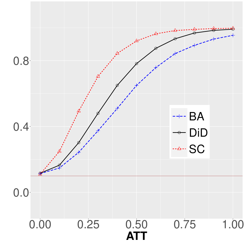
(a) 10%

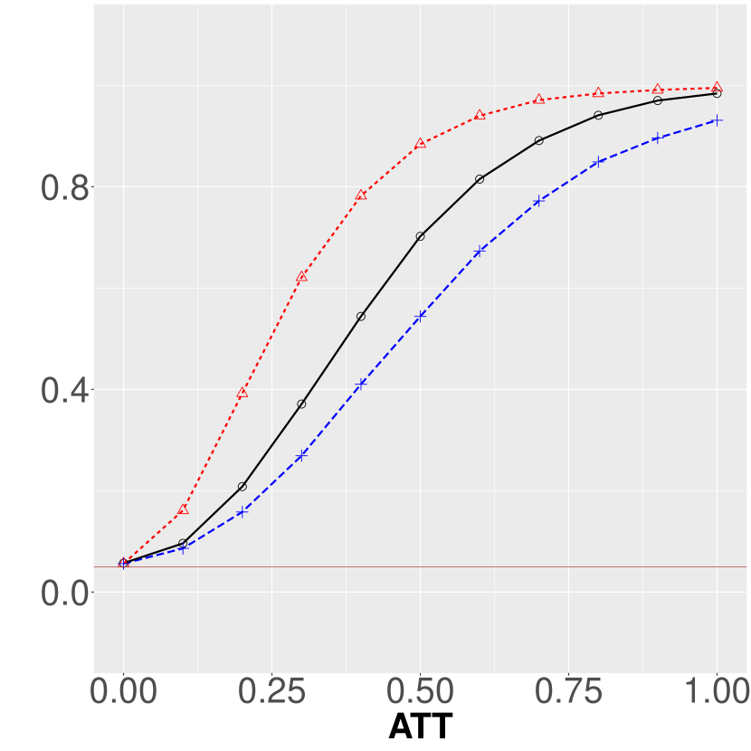
(b) 5%

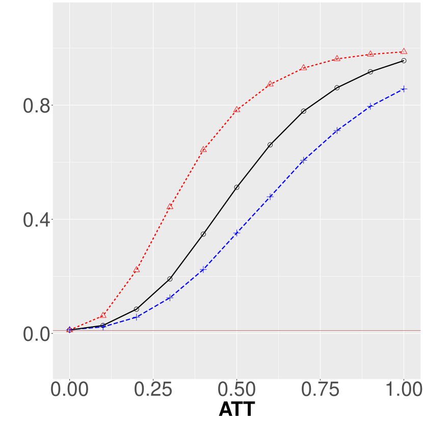
(c) 1%

Figure S.6: Power Curves - DGP SC-BA, $\mathcal{T},T=25$.

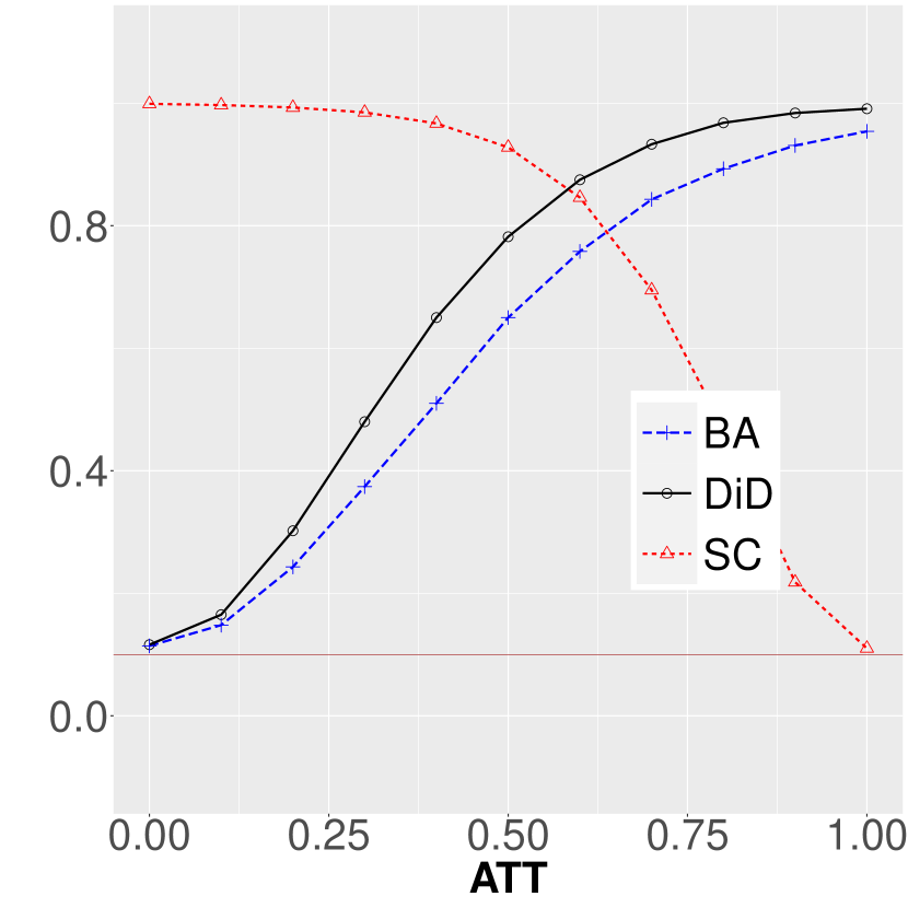
(a) 10%

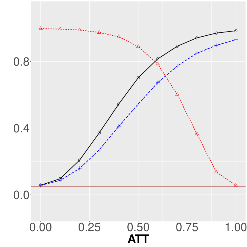
(b) 5%

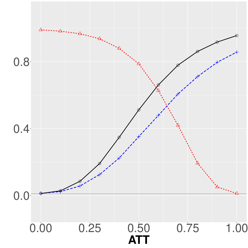
(c) 1%

Figure S.7: Power Curves - DGP BA, $\mathcal{T},T=25$.

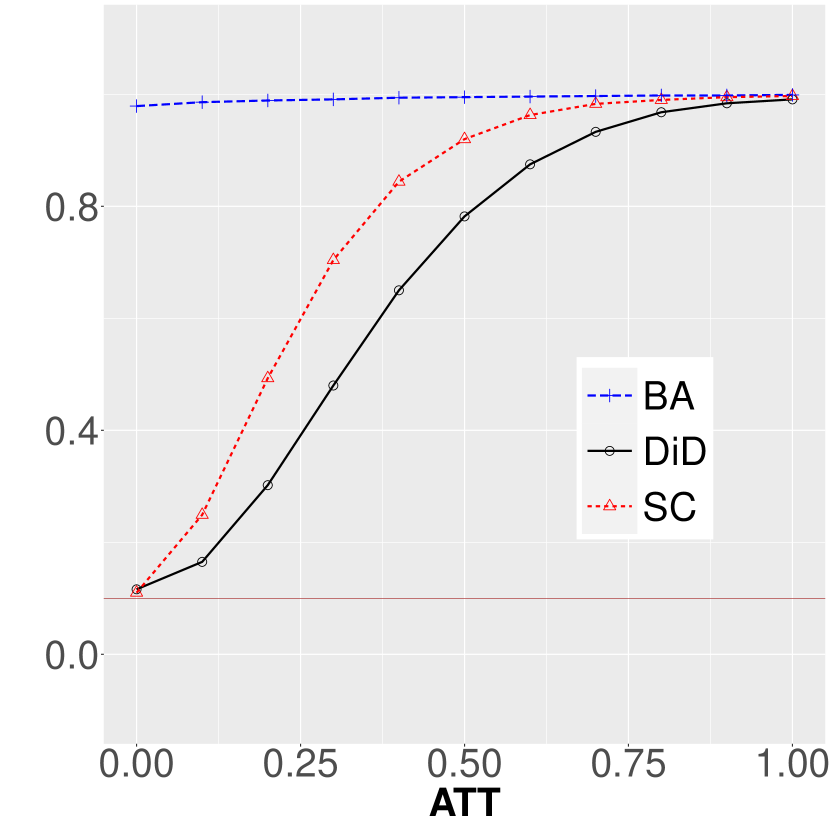
(a) 10%

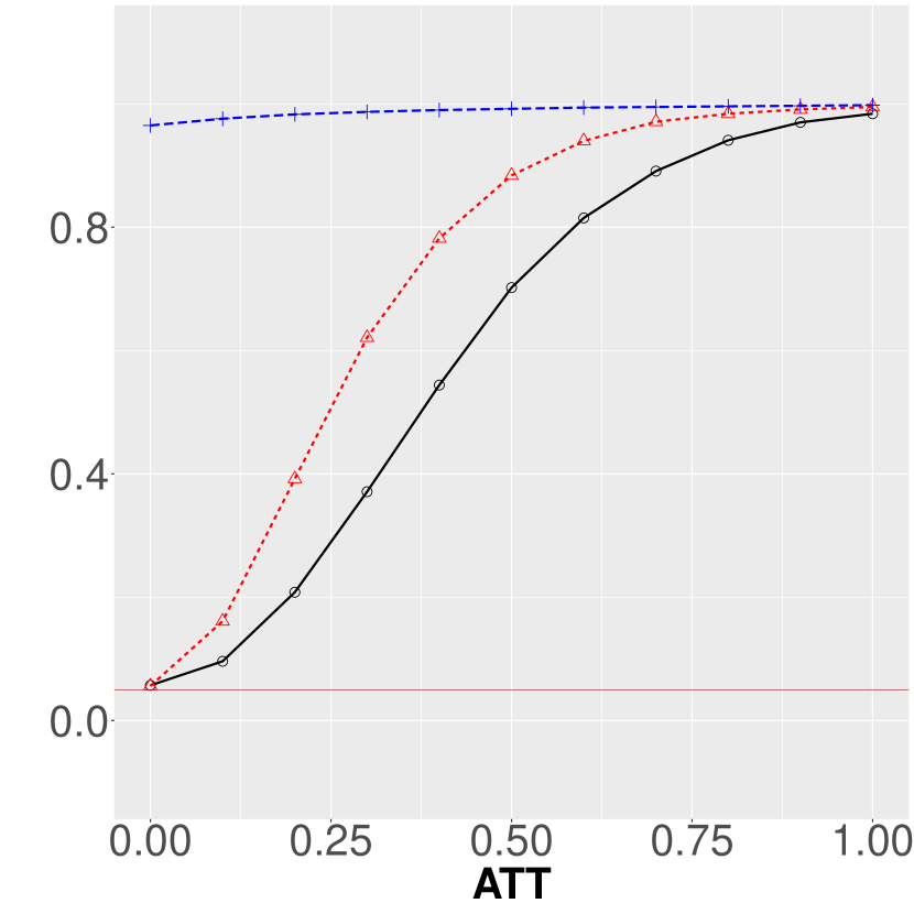
(b) 5%

(c) 1%

Figure S.8: Power Curves - DGP SC, $\mathcal{T},T=25$.

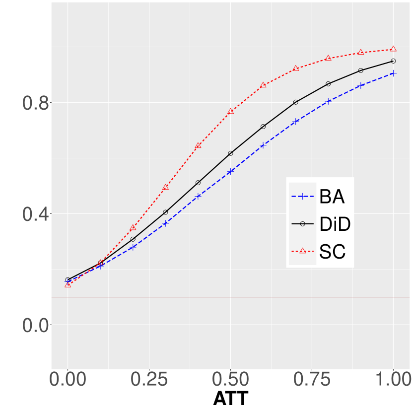
(a) 10%

(b) 5%

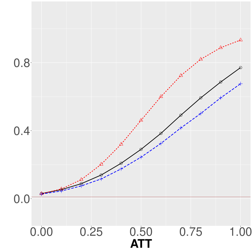
(c) 1%

Figure S.9: Power Curves - DGP PT-NA (A), $\mathcal{T},T=25$.

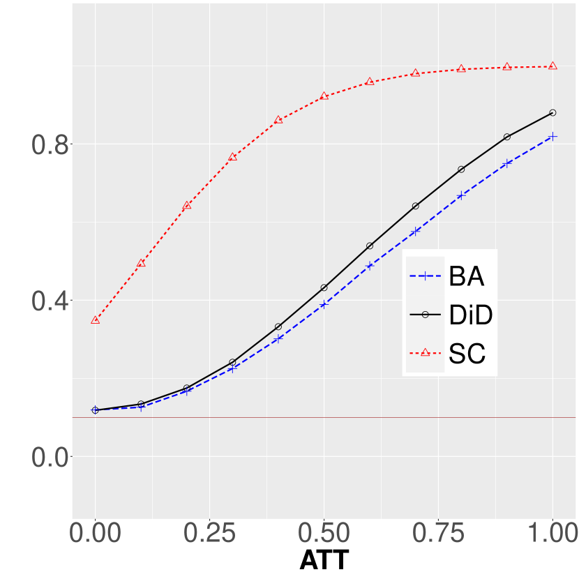
(a) 10%

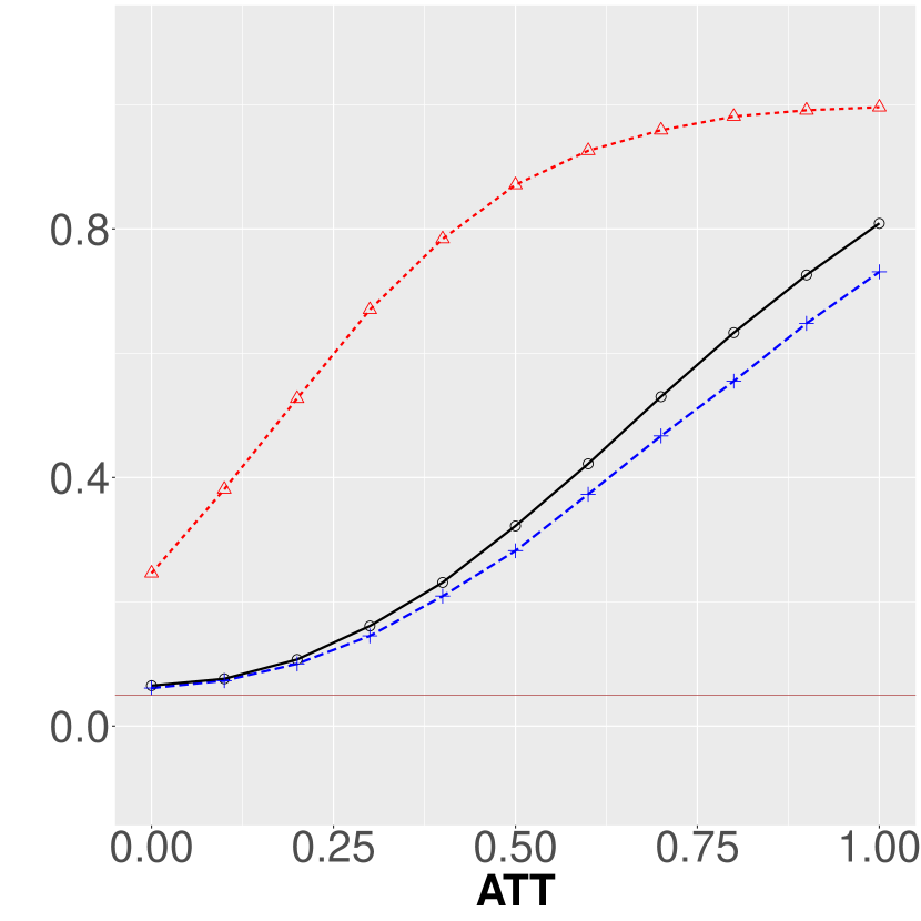
(b) 5%

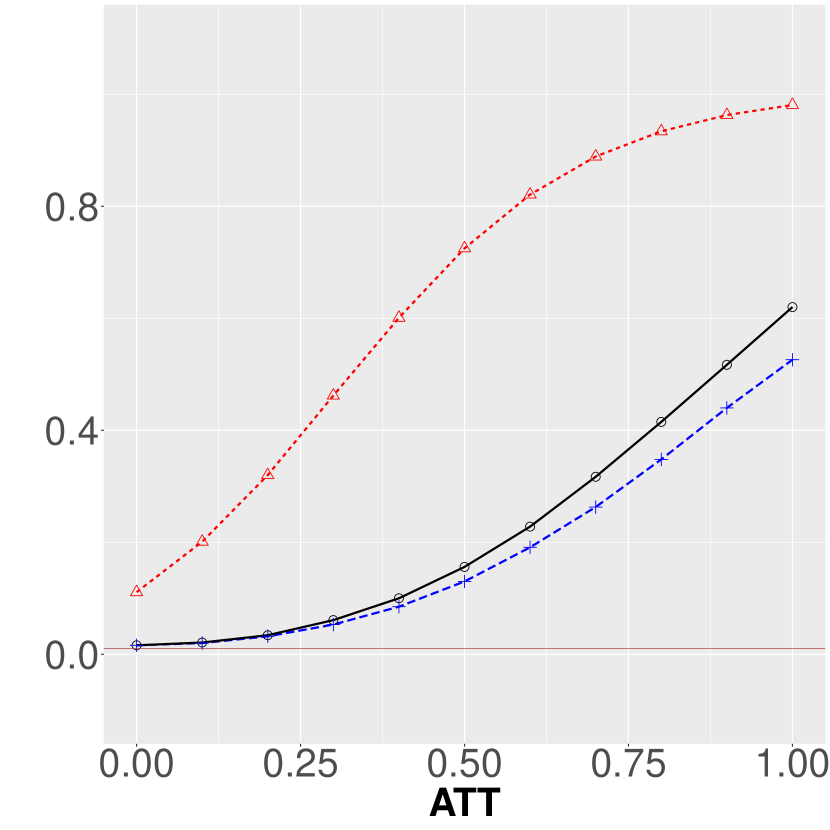
(c) 1%

Figure S.10: Power Curves - DGP PT-NA (B), $\mathcal{T},T=25$.

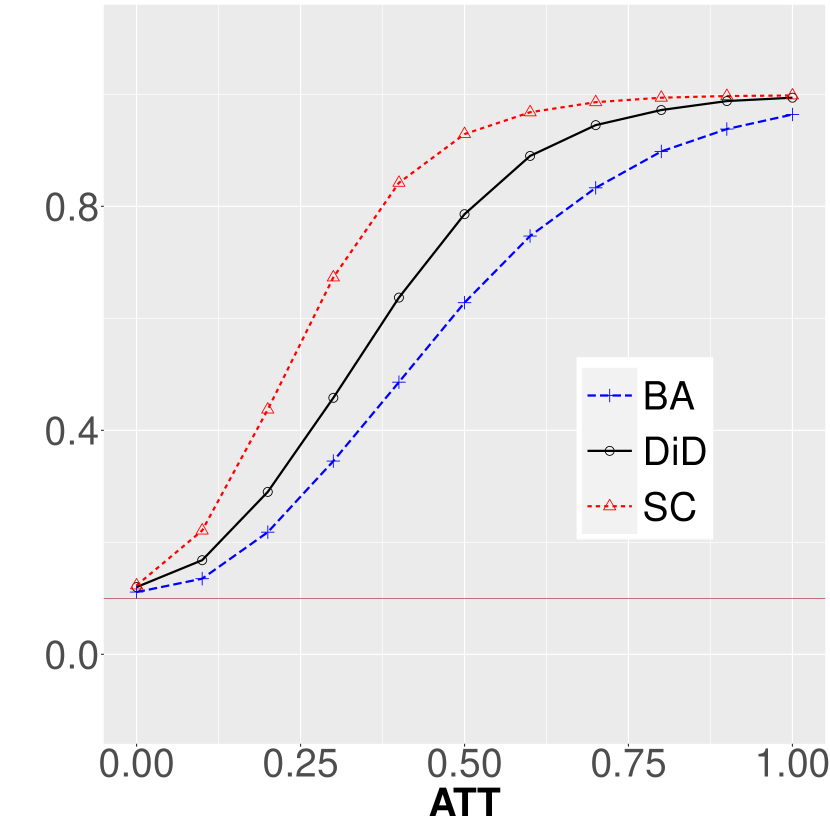
(a) 10%

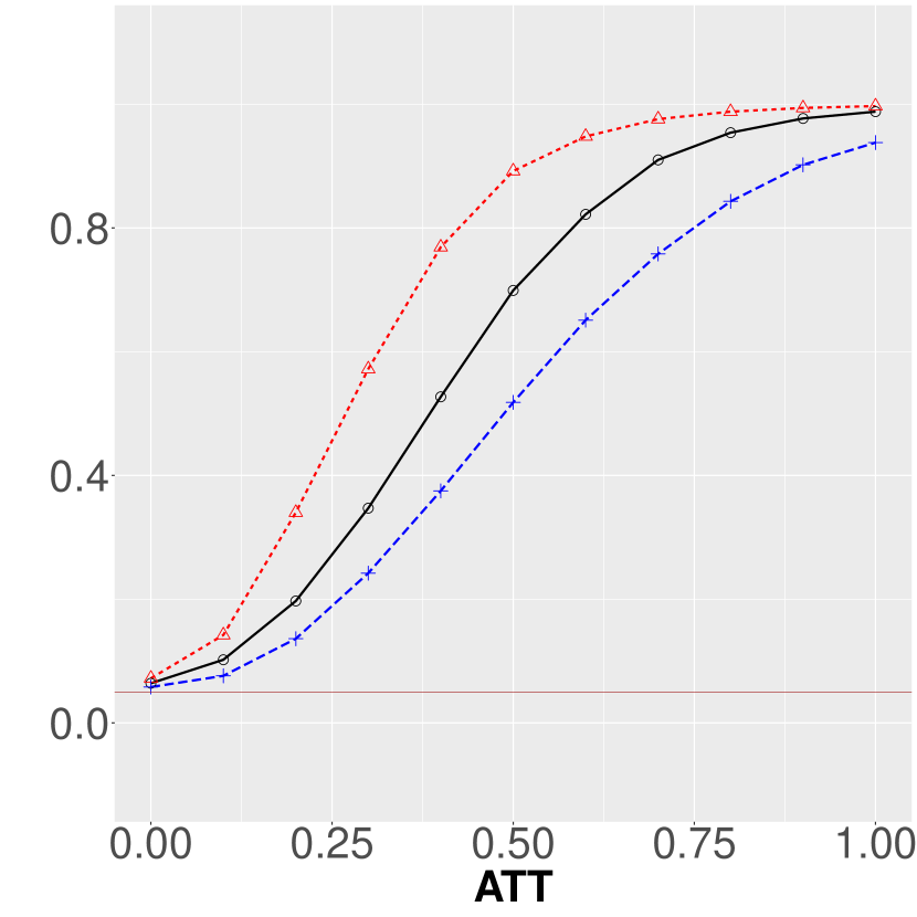
(b) 5%

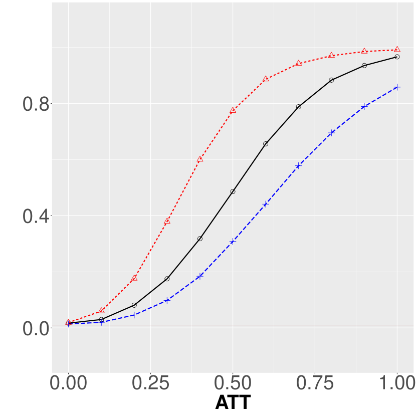
(c) 1%

Figure S.11: Power Curves - DGP GARCH(1,1), $\mathcal{T},T=25$.

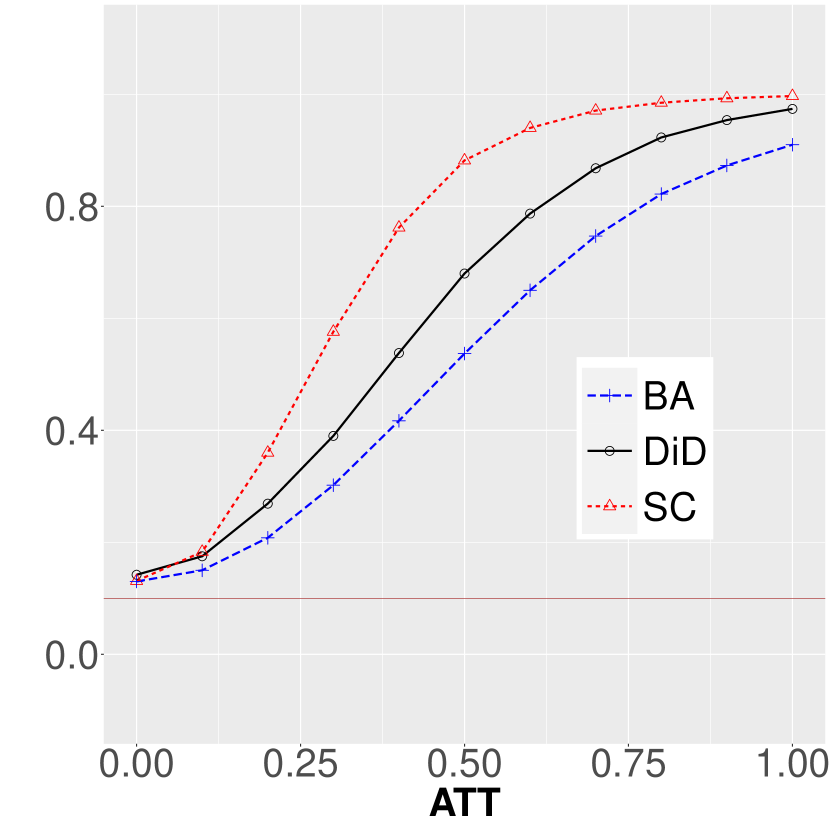
(a) 10%

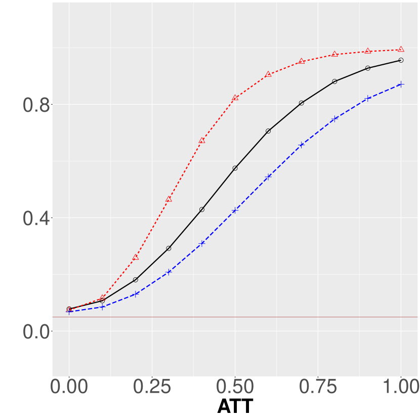
(b) 5%

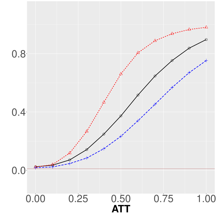
(c) 1%

Figure S.12: Power Curves - DGP MA(1), $\mathcal{T},T=25$.

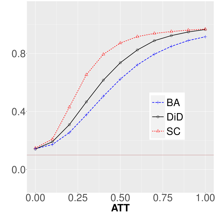
(a) 10%

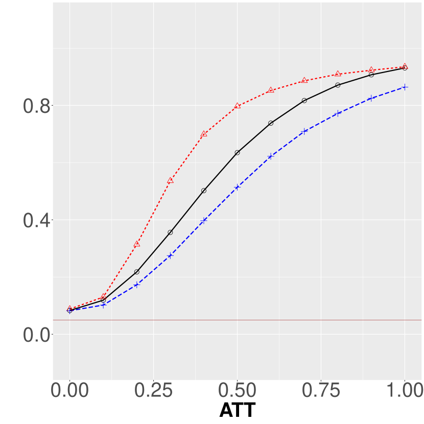
(b) 5%

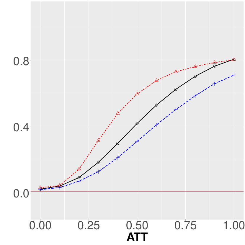
(c) 1%

Figure S.13: Power Curves - DGP AR(1), $\mathcal{T},T=25$.

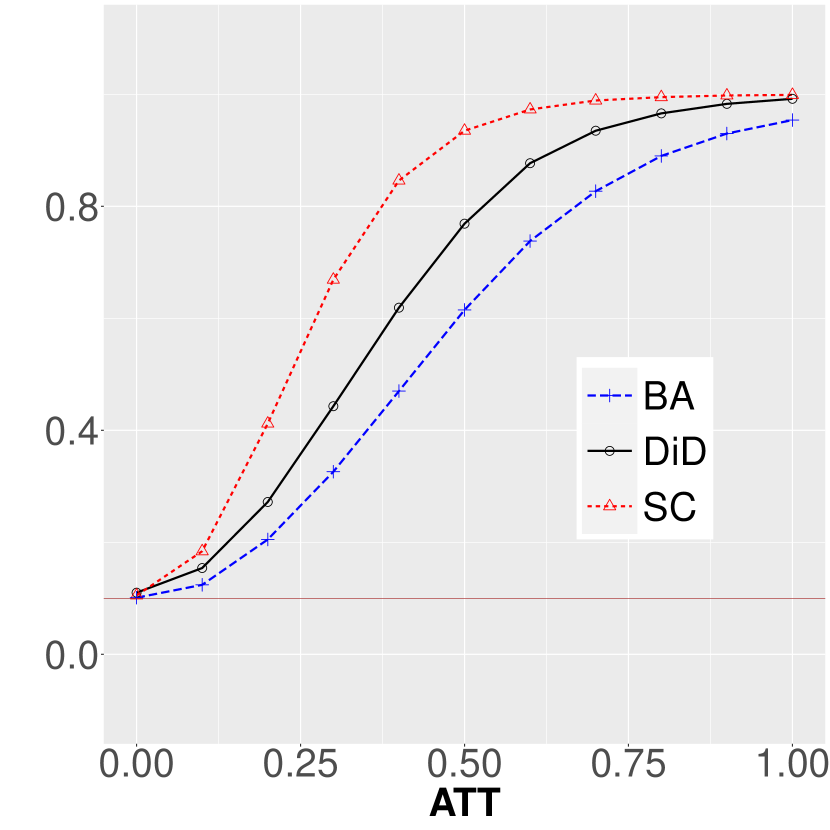
(a) 10%

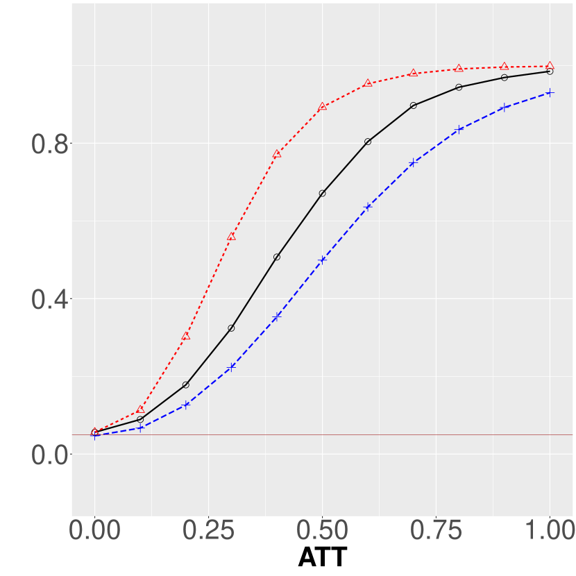
(b) 5%

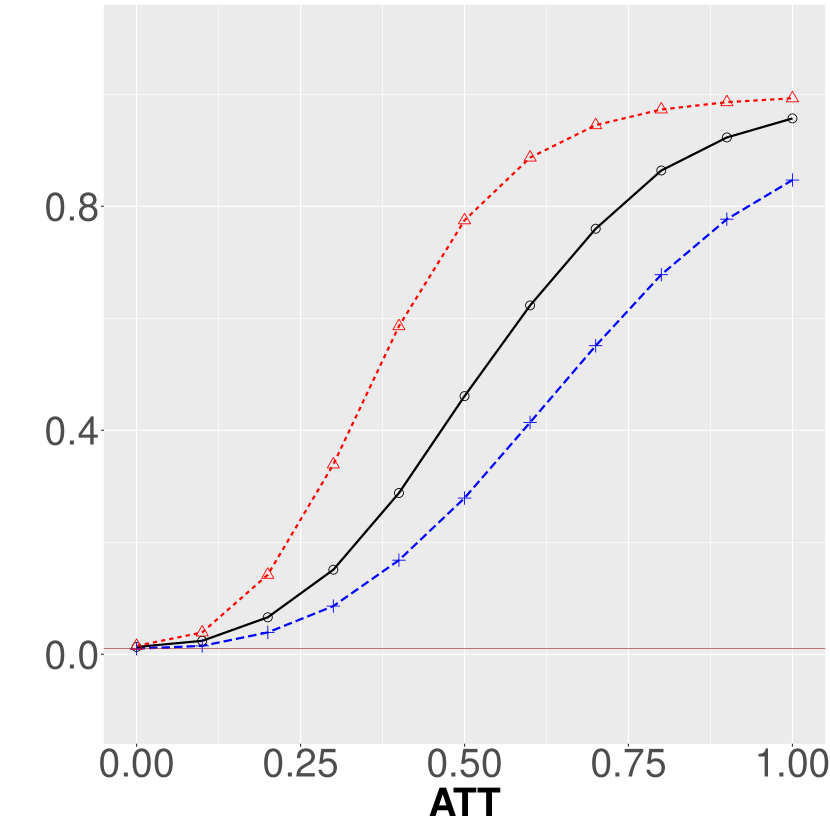
(c) 1%

Figure S.14: Power Curves - DGP U-R, $\mathcal{T},T=25$.

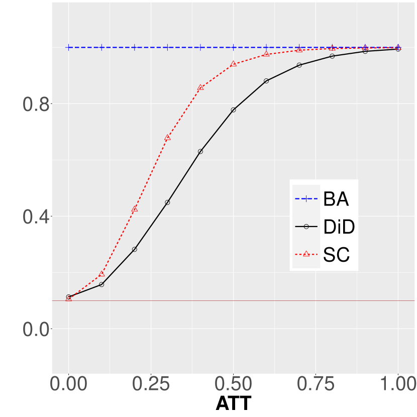
(a) 10%

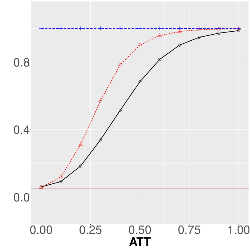
(b) 5%

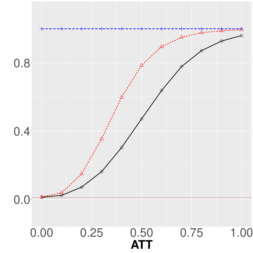
(c) 1%

Figure S.15: Power Curves - DGP Q-T, $\mathcal{T},T=25$.

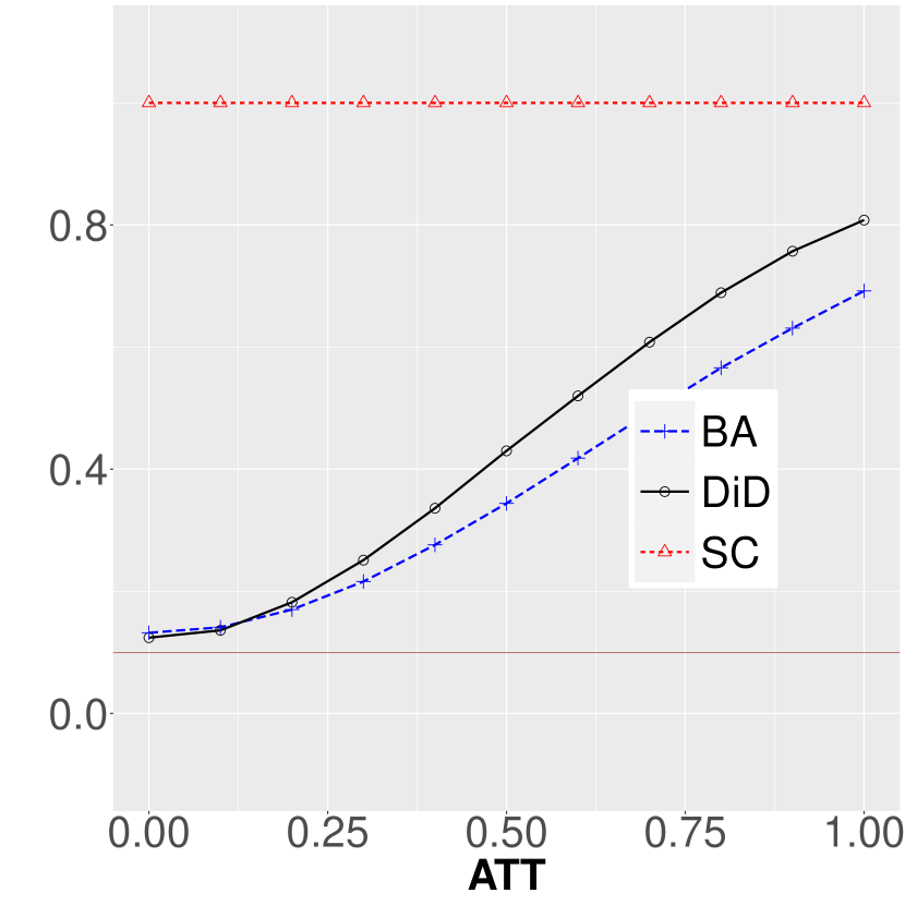
(a) 10%

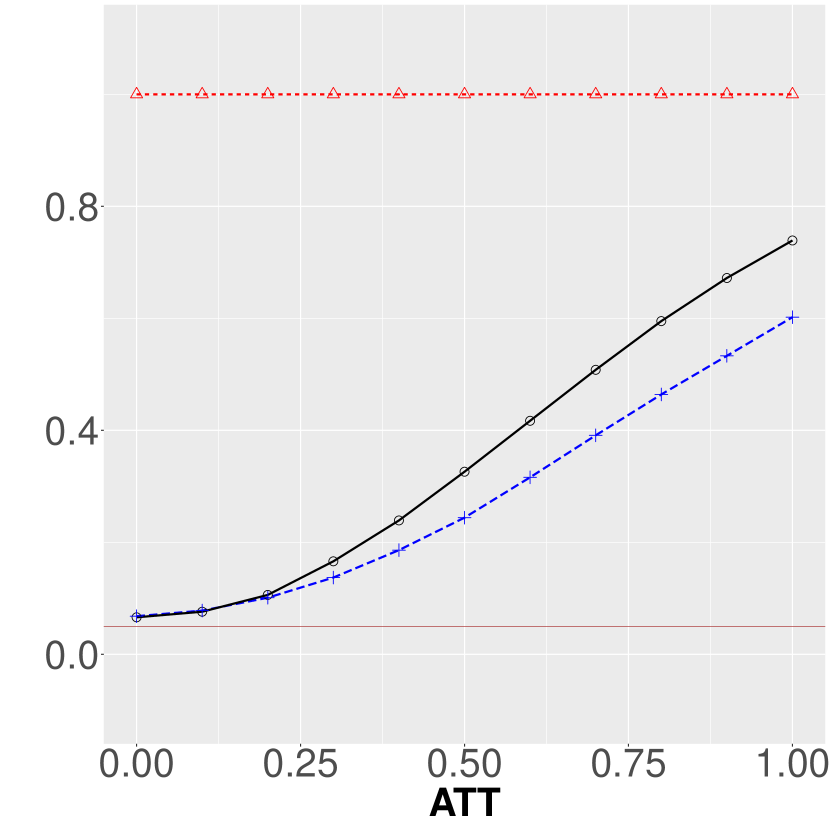
(b) 5%

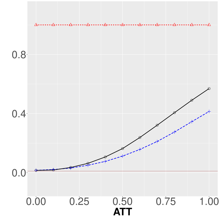
(c) 1%

Figure S.16: Power Curves - DGP T-T, $\mathcal{T},T=25$.

Figures S.6, S.7, S.8, S.9, S.10, S.11, S.12, S.13, S.14, S.15 and S.16 present power curves corresponding to estimator-based $t$-tests of the hypotheses $\mathbb{H}_{o}:\ ATT_{\omega,T}=0.0\text{ vs. }\mathbb{H}_{a}:ATT_{\omega,T}\neq 0.0$. Overall, the power curves continue to reflect the robustness of the $T$-DiD across interesting settings and its ability to detect significant treatment effects. One also observes the failure of either the SC or BA to meaningfully control size under $\mathbb{H}_{o}$, have power under $\mathbb{H}_{a}$, or both whenever any of the stringent conditions under which they hold is violated.

S.5.4 Testing identification

This section examines the empirical sizes and power performance of the family of over-identifying restrictions and pre-trends tests. As both types of tests are based on estimates of $ATT$ on some (sub-)sample, this gives rise to over-identifying restrictions tests id.BA, id.DiD, and id.SC and pre-tests pt.BA, pt.DiD, and pt.SC where the prefixes “id” and “pt” denote over-identifying restrictions and pre-trends tests, respectively using the prefixed estimator DiD, SC, or BA. Pre-trends tests are conducted using approximately, half of pre-treatment periods as a “pre-treatment” period and the other half as the “post-treatment” period.

Modifications of DGPs PT-NA (A) and (B) via the term $\nu_{t}$ provide the following scenarios for examining over-identifying restrictions and pre-trends identification tests using simulations;

1. DGP idTest I : $\nu_{t}\sim\mathcal{N}\big{(}2.5h|t|^{-0.25},1\big{)}$ if $t\leq-1$ and $\nu_{t}=0$ otherwise, $\alpha_{0}=-\alpha_{1}=0.5$;

2. DGP idTest II : $\nu_{t}\sim\mathcal{N}\big{(}2.5h|t|^{-0.25},1\big{)}$ if $t\geq 1$ and $\nu_{t}=0$ otherwise, $\alpha_{0}=\alpha_{1}=0.5$, $\varphi(t)=\sqrt{2}\mathbbm{1}\{t\geq 4\}$; and

3. DGP idTest III : $\nu_{t}\sim\mathcal{N}\big{(}2.5(1-h(1-\mathrm{sgn}(t))|t|^{-0.25},1\big{)}$, $\alpha_{0}=-\alpha_{1}=0.5$, $\varphi(t)=\sqrt{2}\mathbbm{1}\{t\geq 4\}$.

$ATT=0.0$ thus, a “treated” unit is as good as a “control” unit. For the comparison of tests of identification, the $t$-test version of the over-identifying restrictions test is used since there are only two candidate controls. Thus, both units are candidate controls for the over-identifying restrictions tests; one unit serves as the “treated unit” while the other serves as a “control unit” for pre-trends tests.

In all three DGPs above, identification in the $T$-DiD context holds when $h=0$. Both id.DiD and pt.DiD should control size in DGPs idTest I and idTest II while only id.DiD is expected to control size in DGP idTest III. In fact, both Assumptions 1 and 2 are individually violated in DGP idTest III but DiD-identification holds – see Remark 2.3. For $h\in(0,1]$ in (1) DGP idTest I, violations of DiD identification occur in the pre-treatment period (which can be picked up by the pt.DiD), (2) DGP idTest II, violations occur in the post-treatment period which cannot be picked up the pt.DiD, and (3) violations occur in both pre- and post-treatment periods.

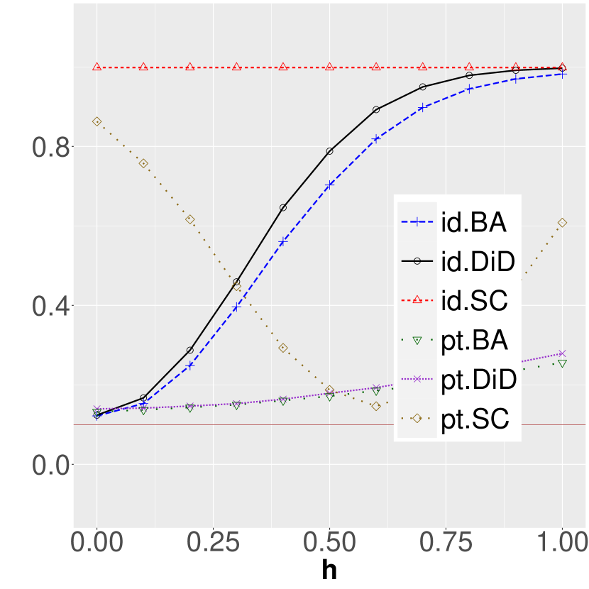
(a) 10%

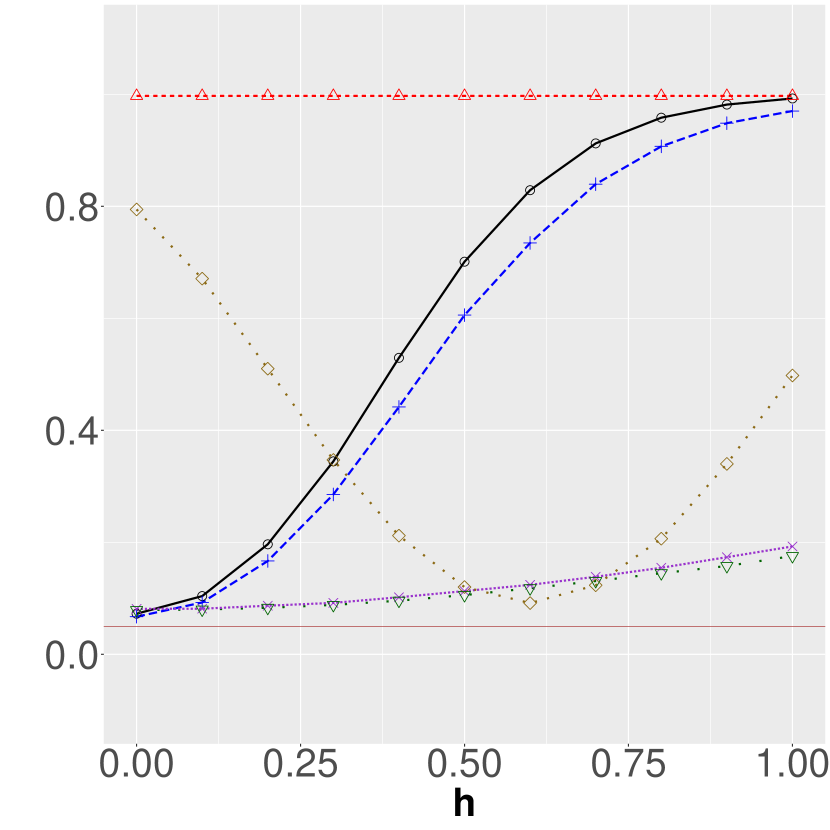
(b) 5%

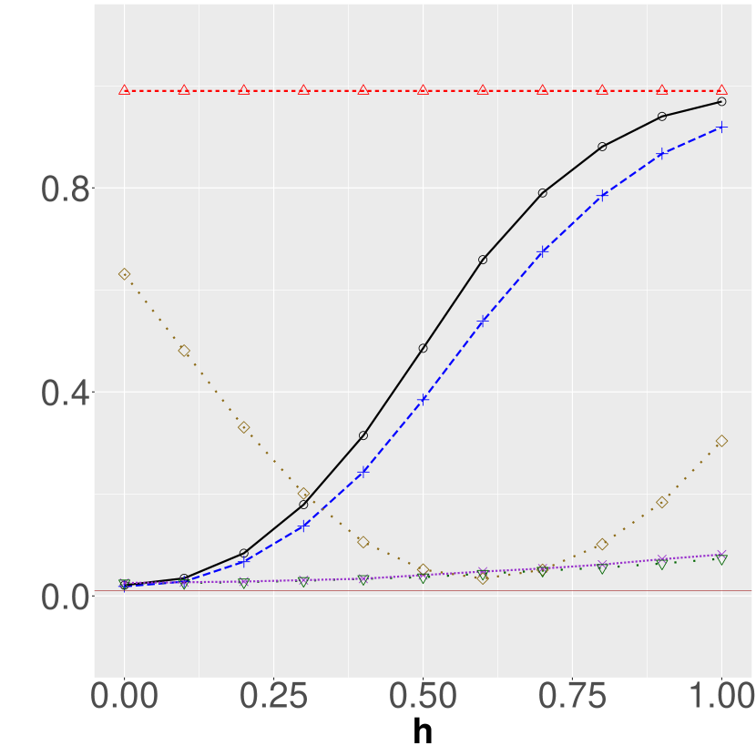
(c) 1%

Figure S.17: Power Curves - DGP idTest I, $\mathcal{T},T=25$.

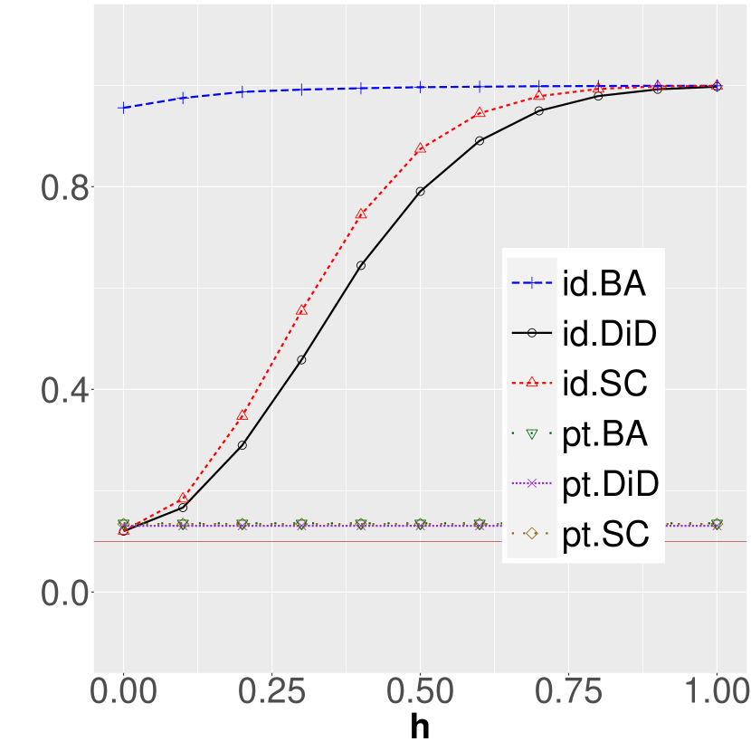
(a) 10%

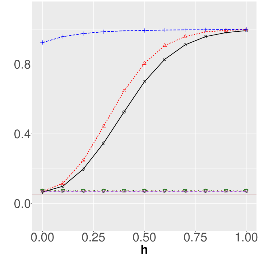
(b) 5%

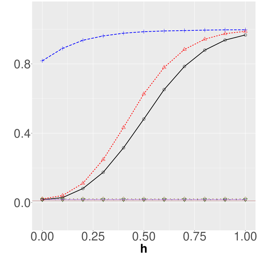
(c) 1%

Figure S.18: Power Curves - DGP idTest II, $\mathcal{T},T=25$.

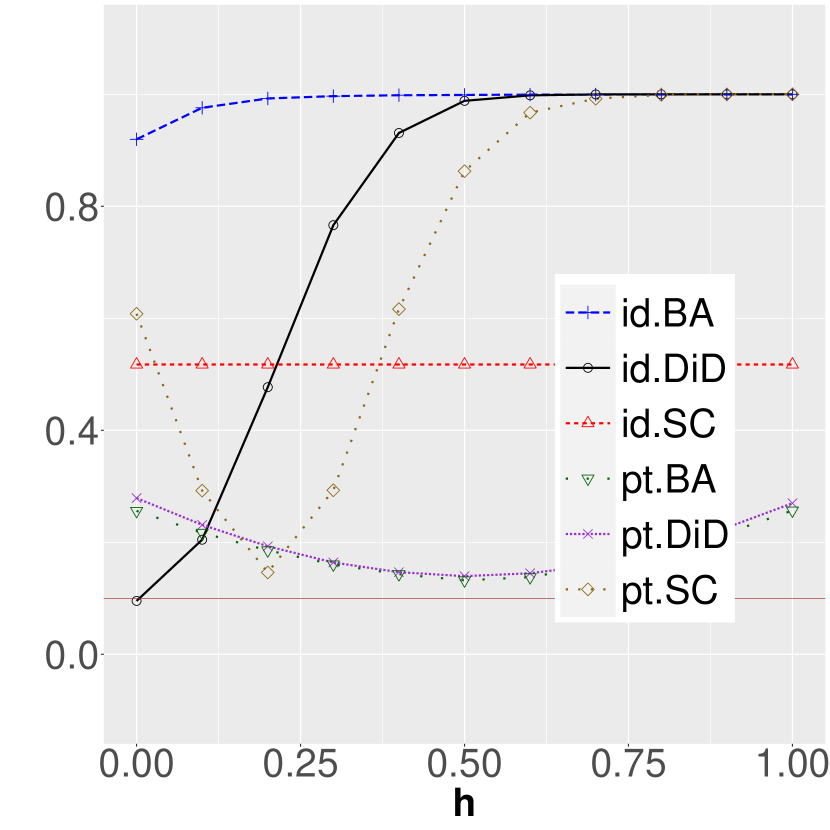
(a) 10%

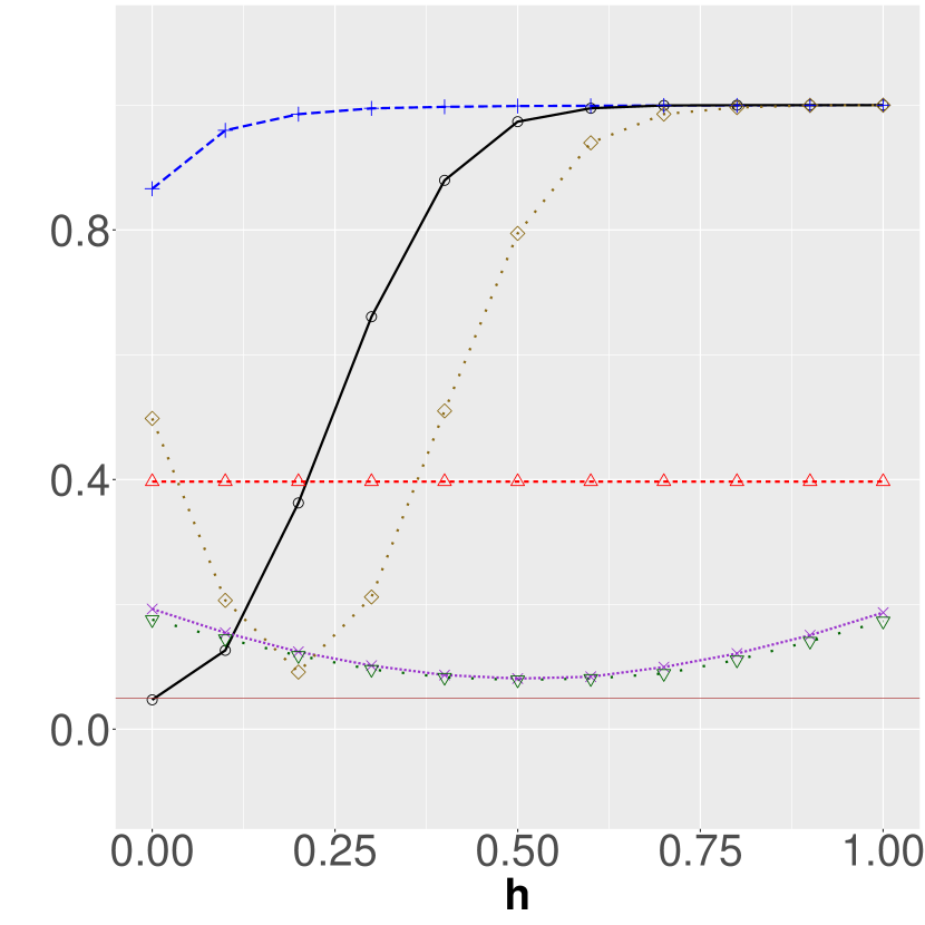
(b) 5%

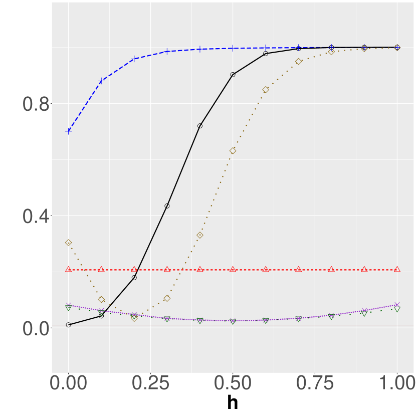
(c) 1%

Figure S.19: Power Curves - DGP idTest III, $\mathcal{T},T=25$.

Figures S.17, S.18 and S.19 present power curves to compare all six candidate tests of identification. As expected, over-identifying restrictions tests based on the BA and SC continue to bear the drawbacks of the respective estimators on which they are based. For example, id.BA jointly controls size meaningfully and has non-trivial power in Figure S.17 but not in Figure S.18 whereas the contrary holds for id.SC. All pre-tests have trivial power, fail to control size meaningfully, or both in Figures S.17, S.18 and S.19. In sum, this short simulation exercise demonstrates the reliability of the DiD-based over-identifying restrictions test of identification even in scenarios, such as DGP idTest II where pre-tests do not help detect violations of ATT.

S.5.5 Heterogeneous Treatment Effects

This section provides more simulation results. The DGPs remain the same but $ATT(t)$ is heterogeneous in $t$ and $ATT_{\omega,T}$ varies with $T$:

$$ATT(t)=\begin{cases}\sin(t)/\pi&\text{ if }t\geq 1\\ 0&\text{ otherwise}\end{cases}.$$

With the choice of the uniform weighting scheme, the sequence of ATT parameters (indexed by $T$) is given by $ATT_{\omega,T}=(\pi T)^{-1}\sum_{t=1}^{T}\sin(t)$. This scenario helps to examine the performance of the DiD when the parameter of interest varies with $T$.

Table S.5: Simulation - $ATT(t)=\sin(t)/\pi,\ t\geq 1$

	$T,\mathcal{T}$	DiD	SC	BA	DiD	SC	BA	DiD	SC	BA
DGP SC-BA		MB			MAD			RMSE
	25	0.002	0.002	0.001	0.14	0.096	0.175	0.216	0.151	0.280
	50	-0.001	0.000	-0.001	0.101	0.070	0.129	0.153	0.107	0.202
	100	0.000	0.000	-0.001	0.072	0.051	0.094	0.108	0.077	0.142
	200	0.001	0.001	0.002	0.051	0.036	0.066	0.076	0.053	0.100
	400	0.000	0.000	0.000	0.037	0.025	0.047	0.054	0.038	0.070
		Rej. 1%			Rej. 5%			Rej. 10%
	25	0.010	0.007	0.011	0.048	0.035	0.050	0.100	0.077	0.103
	50	0.009	0.004	0.009	0.043	0.035	0.049	0.092	0.077	0.102
	100	0.006	0.005	0.008	0.042	0.035	0.048	0.089	0.08	0.096
	200	0.006	0.004	0.008	0.041	0.031	0.044	0.089	0.071	0.091
	400	0.008	0.005	0.008	0.041	0.035	0.043	0.089	0.076	0.090
DGP BA		MB			MAD			RMSE
	25	0.002	-0.998	0.001	0.140	0.997	0.175	0.216	1.009	0.280
	50	-0.001	-1.000	-0.001	0.101	1.000	0.129	0.153	1.006	0.202
	100	0.000	-1.000	-0.001	0.072	1.000	0.094	0.108	1.003	0.142
	200	0.001	-0.999	0.002	0.051	0.999	0.066	0.076	1.001	0.100
	400	0.000	-1.000	0.000	0.037	1.000	0.047	0.054	1.001	0.070
		Rej. 1%			Rej. 5%			Rej. 10%
	25	0.010	0.989	0.011	0.048	0.997	0.050	0.100	0.999	0.103
	50	0.009	1.000	0.009	0.043	1.000	0.049	0.092	1.000	0.102
	100	0.006	1.000	0.008	0.042	1.000	0.048	0.089	1.000	0.096
	200	0.006	1.000	0.008	0.041	1.000	0.044	0.089	1.000	0.091
	400	0.008	1.000	0.008	0.041	1.000	0.043	0.089	1.000	0.090
DGP SC		MB			MAD			RMSE
	25	0.002	0.002	1.246	0.14	0.096	1.248	0.216	0.151	1.277
	50	-0.001	0.000	1.328	0.101	0.07	1.329	0.153	0.107	1.343
	100	0.000	0.000	1.371	0.072	0.051	1.372	0.108	0.077	1.378
	200	0.001	0.001	1.395	0.051	0.036	1.393	0.076	0.053	1.398
	400	0.000	0.000	1.404	0.037	0.025	1.404	0.054	0.038	1.406
		Rej. 1%			Rej. 5%			Rej. 10%
	25	0.010	0.007	0.921	0.048	0.035	0.965	0.100	0.077	0.979
	50	0.009	0.004	0.992	0.043	0.035	0.996	0.092	0.077	0.998
	100	0.006	0.005	0.999	0.042	0.035	1.000	0.089	0.080	1.000
	200	0.006	0.004	1.000	0.041	0.031	1.000	0.089	0.071	1.000
	400	0.008	0.005	1.000	0.041	0.035	1.000	0.089	0.076	1.000

Table S.6: Simulation - $ATT(t)=\sin(t)/\pi,\ t\geq 1$

	$T,\mathcal{T}$	DiD	SC	BA	DiD	SC	BA	DiD	SC	BA
DGP PT-NA (A)		MB			MAD			RMSE
	25	0.177	0.089	0.176	0.27	0.179	0.294	0.397	0.265	0.436
	50	0.109	0.055	0.109	0.185	0.127	0.201	0.273	0.187	0.302
	100	0.063	0.03	0.062	0.128	0.087	0.139	0.19	0.129	0.212
	200	0.037	0.018	0.037	0.089	0.061	0.099	0.132	0.090	0.147
	400	0.023	0.011	0.023	0.063	0.043	0.068	0.092	0.064	0.102
		Rej. 1%			Rej. 5%			Rej. 10%
	25	0.027	0.025	0.026	0.089	0.075	0.086	0.154	0.132	0.147
	50	0.019	0.017	0.016	0.072	0.067	0.072	0.133	0.12	0.128
	100	0.016	0.014	0.015	0.064	0.052	0.068	0.12	0.099	0.124
	200	0.013	0.010	0.011	0.061	0.048	0.058	0.113	0.100	0.114
	400	0.011	0.010	0.011	0.054	0.047	0.053	0.102	0.096	0.104
DGP PT-NA (B)		MB			MAD			RMSE
	25	0.001	0.287	0	0.241	0.294	0.269	0.356	0.381	0.399
	50	0.001	0.246	0.001	0.168	0.248	0.187	0.25	0.304	0.282
	100	-0.002	0.205	-0.002	0.121	0.206	0.134	0.18	0.241	0.202
	200	-0.001	0.175	-0.001	0.085	0.175	0.095	0.126	0.196	0.142
	400	0.001	0.148	0.001	0.06	0.148	0.067	0.089	0.161	0.099
		Rej. 1%			Rej. 5%			Rej. 10%
	25	0.015	0.1	0.014	0.06	0.227	0.058	0.112	0.327	0.115
	50	0.012	0.13	0.01	0.051	0.288	0.05	0.100	0.397	0.105
	100	0.011	0.17	0.009	0.05	0.361	0.055	0.097	0.482	0.105
	200	0.009	0.259	0.01	0.048	0.486	0.045	0.099	0.610	0.096
	400	0.009	0.392	0.008	0.045	0.633	0.045	0.095	0.749	0.098
DGP GARCH(1,1)		MB			MAD			RMSE
	25	0.004	0.001	-0.003	0.141	0.098	0.177	0.214	0.154	0.275
	50	0.001	0.000	0.002	0.102	0.072	0.13	0.152	0.107	0.199
	100	0.000	0.000	0.000	0.071	0.051	0.092	0.108	0.077	0.141
	200	0.000	0.000	0.000	0.052	0.037	0.066	0.077	0.054	0.099
	400	0.000	0.000	0.000	0.036	0.026	0.047	0.054	0.038	0.071
		Rej. 1%			Rej. 5%			Rej. 10%
	25	0.013	0.012	0.010	0.055	0.051	0.05	0.106	0.098	0.102
	50	0.010	0.006	0.009	0.045	0.037	0.048	0.094	0.081	0.097
	100	0.008	0.007	0.008	0.047	0.039	0.046	0.094	0.081	0.091
	200	0.008	0.005	0.007	0.045	0.036	0.041	0.087	0.079	0.088
	400	0.006	0.005	0.008	0.041	0.035	0.042	0.086	0.08	0.092

Table S.7: Simulation - $ATT(t)=\sin(t)/\pi,\ t\geq 1$

	$T,\mathcal{T}$	DiD	SC	BA	DiD	SC	BA	DiD	SC	BA
DGP MA(1)		MB			MAD			RMSE
	25	0.005	0.003	-0.002	0.174	0.119	0.218	0.269	0.19	0.347
	50	-0.001	0.000	-0.002	0.128	0.088	0.164	0.192	0.134	0.251
	100	-0.001	0.000	-0.001	0.091	0.065	0.118	0.135	0.096	0.178
	200	0.001	0.001	0.001	0.064	0.045	0.083	0.095	0.067	0.125
	400	0.000	0.000	0.000	0.045	0.032	0.058	0.067	0.048	0.088
		Rej. 1%			Rej. 5%			Rej. 10%
	25	0.022	0.018	0.015	0.072	0.061	0.065	0.132	0.113	0.122
	50	0.014	0.009	0.015	0.066	0.051	0.064	0.121	0.102	0.118
	100	0.012	0.010	0.010	0.058	0.052	0.054	0.114	0.103	0.113
	200	0.013	0.010	0.012	0.054	0.051	0.054	0.105	0.101	0.109
	400	0.011	0.011	0.009	0.051	0.049	0.053	0.103	0.100	0.110
DGP AR(1)		MB			MAD			RMSE
	25	-0.009	-0.031	-0.009	0.162	0.109	0.207	0.250	0.181	0.322
	50	-0.007	-0.017	-0.006	0.110	0.076	0.145	0.167	0.118	0.216
	100	-0.004	-0.01	-0.004	0.076	0.053	0.100	0.113	0.081	0.146
	200	-0.001	-0.005	-0.001	0.052	0.036	0.068	0.078	0.055	0.102
	400	-0.001	-0.003	-0.001	0.036	0.026	0.047	0.054	0.039	0.071
		Rej. 1%			Rej. 5%			Rej. 10%
	25	0.020	0.027	0.018	0.072	0.075	0.075	0.132	0.128	0.135
	50	0.015	0.015	0.016	0.064	0.056	0.067	0.118	0.105	0.126
	100	0.012	0.011	0.012	0.057	0.053	0.058	0.107	0.104	0.112
	200	0.011	0.010	0.015	0.050	0.047	0.060	0.095	0.094	0.110
	400	0.010	0.008	0.011	0.045	0.041	0.057	0.093	0.086	0.113
DGP U-R		MB			MAD			RMSE
	25	-0.009	-0.01	-0.014	0.144	0.099	0.178	0.221	0.156	0.286
	50	-0.007	-0.006	-0.008	0.103	0.072	0.131	0.155	0.108	0.203
	100	-0.004	-0.004	-0.005	0.073	0.053	0.094	0.109	0.078	0.143
	200	-0.002	-0.002	-0.002	0.051	0.036	0.066	0.077	0.054	0.100
	400	-0.002	-0.002	-0.002	0.036	0.026	0.047	0.054	0.038	0.071
		Rej. 1%			Rej. 5%			Rej. 10%
	25	0.012	0.010	0.008	0.049	0.043	0.043	0.099	0.085	0.095
	50	0.008	0.005	0.007	0.045	0.036	0.045	0.096	0.078	0.095
	100	0.007	0.006	0.006	0.044	0.038	0.04	0.092	0.082	0.091
	200	0.009	0.005	0.008	0.042	0.038	0.043	0.087	0.079	0.092
	400	0.007	0.005	0.006	0.04	0.035	0.043	0.086	0.074	0.095

Table S.8: Simulation - $ATT(t)=\sin(t)/\pi,\ t\geq 1$

	$T,\mathcal{T}$	DiD	SC	BA	DiD	SC	BA	DiD	SC	BA
DGP Q-T		MB			MAD			RMSE
	25	0.003	0.002	25.998	0.141	0.096	25.998	0.217	0.153	25.999
	50	-0.001	0.000	50.998	0.103	0.070	50.998	0.154	0.107	50.998
	100	-0.001	0.000	100.998	0.073	0.052	100.998	0.108	0.077	100.999
	200	0.001	0.001	201.001	0.050	0.036	201.000	0.076	0.054	201.001
	400	0.000	0.000	401.000	0.036	0.026	401.001	0.054	0.038	401.000
		Rej. 1%			Rej. 5%			Rej. 10%
	25	0.011	0.009	1.000	0.050	0.043	1.000	0.101	0.083	1.000
	50	0.009	0.005	1.000	0.046	0.034	1.000	0.092	0.074	1.000
	100	0.008	0.005	1.000	0.043	0.036	1.000	0.092	0.079	1.000
	200	0.009	0.005	1.000	0.043	0.036	1.000	0.087	0.076	1.000
	400	0.007	0.005	1.000	0.038	0.034	1.000	0.084	0.073	1.000
DGP T-T		MB			MAD			RMSE
	25	0.075	25.080	0.080	0.271	25.083	0.346	0.432	25.082	0.576
	50	0.032	50.033	0.042	0.202	50.035	0.252	0.308	50.034	0.403
	100	0.017	100.019	0.017	0.140	100.021	0.182	0.215	100.019	0.283
	200	0.012	200.012	0.011	0.101	200.013	0.131	0.151	200.012	0.200
	400	0.002	400.002	0.001	0.073	400.001	0.093	0.108	400.002	0.140
		Rej. 1%			Rej. 5%			Rej. 10%
	25	0.012	1.000	0.016	0.057	1.000	0.064	0.112	1.000	0.124
	50	0.011	1.000	0.011	0.049	1.000	0.054	0.104	1.000	0.108
	100	0.009	1.000	0.009	0.044	1.000	0.046	0.091	1.000	0.097
	200	0.007	1.000	0.009	0.040	1.000	0.046	0.087	1.000	0.093
	400	0.008	1.000	0.008	0.043	1.000	0.043	0.090	1.000	0.096

Generally, Tables S.5, S.6, S.7 and S.8 confirm results presented in Appendix S.5 in the main text. The DiD performs well across all settings considered in the DGPs, whereas the SC and BA are very sensitive to deviations from the stringent conditions they require. $ATT(t)$ is heterogeneous across post-treatment periods, and the target parameter varies with $T$ and does not impact the performance of the DiD.

References

- [1] Alberto Abadie “Semiparametric difference-in-differences estimators” In The Review of Economic Studies 72.1 Oxford University Press, 2005, pp. 1–19
- [2] Alberto Abadie “Using synthetic controls: Feasibility, data requirements, and methodological aspects” In Journal of Economic Literature 59.2 American Economic Association 2014 Broadway, Suite 305, Nashville, TN 37203-2425, 2021, pp. 391–425
- [3] Alberto Abadie, Alexis Diamond and Jens Hainmueller “Synthetic control methods for comparative case studies: Estimating the effect of California’s tobacco control program” In Journal of the American Statistical Association 105.490 Taylor & Francis, 2010, pp. 493–505
- [4] Alberto Abadie and Javier Gardeazabal “The economic costs of conflict: A case study of the Basque Country” In American Economic Review 93.1, 2003, pp. 113–132
- [5] Daron Acemoglu, Suresh Naidu, Pascual Restrepo and James A Robinson “Democracy does cause growth” In Journal of Political Economy 127.1 University of Chicago Press Chicago, IL, 2019, pp. 47–100
- [6] Joshua D Angrist, Òscar Jordà and Guido M Kuersteiner “Semiparametric estimates of monetary policy effects: String theory revisited” In Journal of Business & Economic Statistics 36.3 Taylor & Francis, 2018, pp. 371–387
- [7] Joshua D Angrist and Jorn-Steffen Pischke “Mostly Harmless Econometrics: An Empiricist’s Companion” Princeton University Press, 2008
- [8] Dmitry Arkhangelsky, Susan Athey, David A Hirshberg, Guido W Imbens and Stefan Wager “Synthetic difference-in-differences” In American Economic Review 111.12 American Economic Association 2014 Broadway, Suite 305, Nashville, TN 37203, 2021, pp. 4088–4118
- [9] Christophe Bellégo, David Benatia and Vincent Dortet-Bernadet “The chained difference-in-differences” In Journal of Econometrics Elsevier, 2024, pp. 105783
- [10] Eli Ben-Michael, Avi Feller and Jesse Rothstein “The augmented synthetic control method” In Journal of the American Statistical Association 116.536 Taylor & Francis, 2021, pp. 1789–1803
- [11] Vanessa A Boese “How (not) to measure democracy” In International Area Studies Review 22.2 SAGE Publications Sage UK: London, England, 2019, pp. 95–127
- [12] Brantly Callaway and Pedro HC Sant’Anna “Difference-in-differences with multiple time periods” In Journal of Econometrics 225.2, 2021, pp. 200–230
- [13] David Card “The impact of the Mariel boatlift on the Miami labor market” In Industrial & Labor Relations Review 43.2 SAGE Publications, 1990, pp. 245–257
- [14] Carlos Carvalho, Ricardo Masini and Marcelo C Medeiros “ArCo: An artificial counterfactual approach for high-dimensional panel time-series data” In Journal of Econometrics 207.2 Elsevier, 2018, pp. 352–380
- [15] Marc K Chan and Simon S Kwok “The PCDID approach: Difference-in-differences when trends are potentially unparallel and stochastic” In Journal of Business & Economic Statistics Taylor & Francis, 2021, pp. 1–18
- [16] Chaoyi Chen and Thanasis Stengos “Threshold nonlinearities and the democracy-growth nexus” In The Econometrics Journal Oxford University Press, 2024, pp. utae006
- [17] Victor Chernozhukov, Kaspar Wuthrich and Yinchu Zhu “A -test for synthetic controls” In arXiv preprint arXiv:1812.10820, 2024
- [18] Victor Chernozhukov, Kaspar Wüthrich and Yinchu Zhu “An exact and robust conformal inference method for counterfactual and synthetic controls” In Journal of the American Statistical Association 116.536 Taylor & Francis, 2021, pp. 1849–1864
- [19] Marco Colagrossi, Domenico Rossignoli and Mario A Maggioni “Does democracy cause growth? A meta-analysis (of 2000 regressions)” In European Journal of Political Economy 61 Elsevier, 2020, pp. 101824
- [20] Michael Coppedge, Amanda B Edgell, Carl Henrik Knutsen and Staffan I Lindberg “Why Democracies Develop and Decline” Cambridge University Press, 2022
- [21] James Davidson “Stochastic Limit Theory: An Introduction for Econometricians” Oxford University Press, 2021
- [22] Clement de Chaisemartin and Xavier D’Haultfœuille “Two-way fixed effects estimators with heterogeneous treatment effects” In American Economic Review 110.9, 2020, pp. 2964–2996
- [23] Robert M De Jong “Central limit theorems for dependent heterogeneous random variables” In Econometric Theory 13.3 Cambridge University Press, 1997, pp. 353–367
- [24] Hristos Doucouliagos and Mehmet Ali Ulubaşoğlu “Democracy and economic growth: A meta-analysis” In American Journal of Political Science 52.1 Wiley Online Library, 2008, pp. 61–83
- [25] Nikolay Doudchenko and Guido W Imbens “Balancing, regression, difference-in-differences and synthetic control methods: A synthesis” Working Paper, 2016
- [26] Bruno Ferman “Inference in difference-in-differences with few treated units and spatial correlation” In arXiv preprint arXiv:2006.16997, 2020
- [27] Bruno Ferman and Cristine Pinto “Inference in differences-in-differences with few treated groups and heteroskedasticity” In Review of Economics and Statistics 101.3 MIT Press One Rogers Street, Cambridge, MA 02142-1209, USA journals-info …, 2019, pp. 452–467
- [28] Bruno Ferman and Cristine Pinto “Synthetic controls with imperfect pretreatment fit” In Quantitative Economics 12.4 Wiley Online Library, 2021, pp. 1197–1221
- [29] Roberto Stefan Foa, Andrew Klassen, Micheal Slade, Alex Rand and Rosie Collins “The global satisfaction with democracy report 2020” University of Cambridge, 2020
- [30] Joseph Fry “A method of moments approach to asymptotically unbiased synthetic controls” In arXiv preprint arXiv:2312.01209, 2023
- [31] John Gerring, Philip Bond, William T Barndt and Carola Moreno “Democracy and economic growth: A historical perspective” In World Politics 57.3 Cambridge University Press, 2005, pp. 323–364
- [32] Francesco Giavazzi and Guido Tabellini “Economic and political liberalizations” In Journal of Monetary Economics 52.7 Elsevier, 2005, pp. 1297–1330
- [33] Katherine K Grooms “Enforcing the Clean Water Act: The effect of state-level corruption on compliance” In Journal of Environmental Economics and Management 73 Elsevier, 2015, pp. 50–78
- [34] Patrik Guggenberger “A note on the (in) consistency of the test of overidentifying restrictions and the concepts of true and pseudo-true parameters” In Economics Letters 117.3 Elsevier, 2012, pp. 901–904
- [35] Andreas Hagemann “Inference with a single treated cluster” In arXiv preprint arXiv:2010.04076, 2020
- [36] James Douglas Hamilton “Time Series Analysis” Princeton University Press, 1994 URL: https://www.worldcat.org/title/time-series-analysis/oclc/1194970663&referer=brief_results
- [37] Bruce E Hansen “GARCH (1, 1) processes are near epoch dependent” In Economics Letters 36.2 Elsevier, 1991, pp. 181–186
- [38] Bruce E. Hansen “Econometrics” University of Wisconsin, Dept. of Economics, 2021
- [39] Cheng Hsiao, H. Ching and Shui Ki Wan “A panel data approach for program evaluation: Measuring the benefits of political and economic integration of Hong kong with mainland China” In Journal of Applied Econometrics 27.5 Wiley Online Library, 2012, pp. 705–740
- [40] Ariella Kahn-Lang and Kevin Lang “The promise and pitfalls of differences-in-differences: Reflections on 16 and pregnant and other applications” In Journal of Business & Economic Statistics 38.3 Taylor & Francis, 2020, pp. 613–620
- [41] Carl Henrik Knutsen “A business case for democracy: regime type, growth, and growth volatility” In Democratization 28.8 Taylor & Francis, 2021, pp. 1505–1524
- [42] Dirk Kohnert “BTI 2021 - Togo country report: Togo’s political and socio-economic development (2019-2021) [author’s enhanced version]” In BTI project: Shaping Change - Strategies of Development and Transformation ; Political Economy of Africa Gütersloh: Bertelsmann Stiftung, 2021, pp. 1–62
- [43] Jong-Wha Lee and Kwanho Shin “IMF bailouts and moral hazard” In Journal of International Money and Finance 27.5 Elsevier, 2008, pp. 816–830
- [44] Lihua Lei and Timothy Sudijono “Inference for synthetic controls via refined placebo tests” In arXiv preprint arXiv:2401.07152, 2024
- [45] Kathleen T Li “Statistical inference for average treatment effects estimated by synthetic control methods” In Journal of the American Statistical Association 115.532 Taylor & Francis, 2020, pp. 2068–2083
- [46] Michelle Marcus and Pedro HC Sant’Anna “The role of parallel trends in event study settings: An application to environmental economics” In Journal of the Association of Environmental and Resource Economists 8.2 The University of Chicago Press Chicago, IL, 2021, pp. 235–275
- [47] Ricardo Masini and Marcelo C Medeiros “Counterfactual analysis and inference with nonstationary data” In Journal of Business & Economic Statistics 40.1 Taylor & Francis, 2022, pp. 227–239
- [48] Fabrice Murtin and Romain Wacziarg “The democratic transition” In Journal of Economic Growth 19.2 Springer, 2014, pp. 141–181
- [49] WK Newey and KD West “A simple, positive semi-definite, heteroskedasticity and autocorrelation consistent covariance matrix” In Econometrica 55.3, 1987, pp. 703–708
- [50] Daniel Ngo, Keegan Harris, Anish Agarwal, Vasilis Syrgkanis and Zhiwei Steven Wu “Incentive-aware synthetic control: Accurate counterfactual estimation via incentivized exploration” In arXiv preprint arXiv:2312.16307, 2023
- [51] Elias Papaioannou and Gregorios Siourounis “Democratisation and growth” In The Economic Journal 118.532 Oxford University Press Oxford, UK, 2008, pp. 1520–1551
- [52] Torsten Persson “Forms of democracy, policy and economic development” National Bureau of Economic Research Cambridge, Mass., USA, 2005
- [53] Torsten Persson and Guido Tabellini “Democracy and development: The devil in the details” In American Economic Review 96.2 American Economic Association, 2006, pp. 319–324
- [54] Torsten Persson and Guido Tabellini “Democratic capital: The nexus of political and economic change” In American Economic Journal: Macroeconomics 1.2 American Economic Association, 2009, pp. 88–126
- [55] M Hashem Pesaran “Time series and panel data econometrics” Oxford University Press, 2015
- [56] M Hashem Pesaran and Ron P Smith “Counterfactual analysis in macroeconometrics: An empirical investigation into the effects of quantitative easing” In Research in Economics 70.2 Elsevier, 2016, pp. 262–280
- [57] Jonathan Roth, Pedro HC Sant’Anna, Alyssa Bilinski and John Poe “What’s trending in difference-in-differences? A synthesis of the recent econometrics literature” In Journal of Econometrics Elsevier, 2023
- [58] Liyang Sun, Eli Ben-Michael and Avi Feller “Using multiple outcomes to improve the synthetic control method” In arXiv preprint arXiv:2311.16260, 2023
- [59] Wei Tian, Seojeong Lee and Valentyn Panchenko “Synthetic controls with multiple outcomes” In arXiv preprint arXiv:2304.02272, 2024
- [60] Jeffrey M Wooldridge “Econometric Analysis of Cross Section and Panel Data” MIT press, 2010
- [61] Yiqing Xu “Generalized synthetic control method: Causal inference with interactive fixed effects models” In Political Analysis 25.1 Cambridge University Press, 2017, pp. 57–76
- [62] James Davidson “Stochastic Limit Theory: An Introduction for Econometricians” Oxford University Press, 2021
- [63] Holger Dette and Martin Schumann “Testing for equivalence of pre-trends in Difference-in-Differences estimation” In Journal of Business & Economic Statistics Taylor & Francis, 2024, pp. 1–13
- [64] Simon Freyaldenhoven, Christian Hansen and Jesse M Shapiro “Pre-event trends in the panel event-study design” In American Economic Review 109.9, 2019, pp. 3307–38
- [65] Ariella Kahn-Lang and Kevin Lang “The promise and pitfalls of differences-in-differences: Reflections on 16 and pregnant and other applications” In Journal of Business & Economic Statistics 38.3 Taylor & Francis, 2020, pp. 613–620
- [66] WK Newey and KD West “A simple, positive semi-definite, heteroskedasticity and autocorrelation consistent covariance matrix” In Econometrica 55.3, 1987, pp. 703–708
- [67] Jonathan Roth “Pretest with caution: Event-study estimates after testing for parallel trends” In American Economic Review: Insights 4.3, 2022, pp. 305–22
- [68] Jeffrey M Wooldridge “Econometric Analysis of Cross Section and Panel Data” MIT press, 2010