S4D: Streaming 4D Real-World Reconstruction with Gaussians and 3D Control Points

Abstract

Recently, the dynamic scene reconstruction using Gaussians has garnered increased interest. Mainstream approaches typically employ a global deformation field to warp a 3D scene in the canonical space. However, the inherently low-frequency nature of implicit neural fields often leads to ineffective representations of complex motions. Moreover, their structural rigidity can hinder adaptation to scenes with varying resolutions and durations. To overcome these challenges, we introduce a novel approach utilizing discrete 3D control points. This method models local rays physically and establishes a motion-decoupling coordinate system, which effectively merges traditional graphics with learnable pipelines for a robust and efficient local 6-degrees-of-freedom (6-DoF) motion representation. Additionally, we have developed a generalized framework that incorporates our control points with Gaussians. Starting from an initial 3D reconstruction, our workflow decomposes the streaming 4D real-world reconstruction into four independent submodules: 3D segmentation, 3D control points generation, object-wise motion manipulation, and residual compensation. Our experiments demonstrate that this method outperforms existing state-of-the-art 4D Gaussian Splatting techniques on both the Neu3DV and CMU-Panoptic datasets. Our approach also significantly accelerates training, with the optimization of our 3D control points achievable within just 2 seconds per frame on a single NVIDIA 4070 GPU.

1 Introduction

Reconstruction of real-world scenes is a classic question in computer graphics. The recent 3D Gaussian Splatting(3D-GS) [16] work has achieved impressive results with high-quality reconstruction for static scenes. Discrete Gaussians represent the scene with physically meaningful attributes, and the rendering process is realized by "splatting" Gaussians on the image plane. For dynamic scene reconstruction, mainstream GS methods [58, 13, 55, 24] built on the dynamic NeRF’s [31, 32, 34] idea, decomposing motions from the scene in a canonical space and using an implicit neural field to represent the scene’s global motion. However, The implicit neural network’s low-frequency nature and structural inflexibility prevent it from adopting complex motions and scenes of varying resolution and length.

Compared to NeRF, one of the main advantages of 3D-GS is its discrete structure. This ensures that the scene representation, i.e., the Gaussians, is concentrated at influential positions within the scene, avoiding the inefficiency of the global field that wastes representation capability in empty space. The global implicit neural field for deformation also suffers from the identical drawback, as only a tiny part of the scene is dynamic over time; most of it remains static. Thus, discrete local motion representation is promising because it can represent 3D motions locally, precisely, and flexibly.

Previous traditional [47] and learning-based [13] works have attempted to represent local 3D motion in a discrete manner. However, traditional methods face challenging 3D alignment, and learning-based approaches find convergence tricky because too many degrees of freedom(DoF) exist. We approach the problem differently by combining graphics and learnable pipelines. Given that optical flow is the projection of scene flow and that optical flow estimation [35, 43, 46, 19] is mature, we simplify the challenge by designing a subtle local decoupling system. The local 3D motion is decoupled into the observable and hidden portions. While the observable portion is bound with optical flow, the hidden portion remains learnable. We call this new type of motion representation the 3D control point approach.

Based on the 3D motion representation we introduced, we propose a new generalized streaming framework to support 4D real-world reconstruction. Given an initial 3D reconstruction, our workflow decomposes the streaming 4D reconstruction process into distinct submodules: 3D segmentation, 3D control points generation, object-wise motion manipulation, and residual compensation. This methodology prevents topological errors and ensures a compact and robust representation.

Our contributions are highlighted as follows:

• We discretely model the 3D motions of dynamic objects using a novel approach combining graphics and learnable pipelines. This technique effectively decouples the components of objects’ 3D motions; one part is bound to the optical flow, and the other part is acquired through learning. This motion representation, termed “3D control points” enhances convergence speed and reconstruction accuracy.

• We introduce a generalized streaming pipeline that leverages Gaussians and 3D control points to reconstruct 4D real-world scenes. This approach sets a new benchmark, achieving state-of-the-art results on both the Neu3DV and CMU-Panoptic datasets.

2 Related Work

2.1 4D Reconstruction

The recent Neural Radiance Field(NeRF) [29] approach has been demonstrated efficient in scene reconstruction. NeRF utilized a global continuous implicit representation to represent the scene. Subsequent works improved the reconstruction quality by modifying MLP to grid-based structures. For example, Müller et al. [30] introduced an Instant Neural Graphics Primitives method, while Fridovich-Keil et al. [9] presented Plenoxels. Other works like Mip-NeRF [3, 4] modeled rays as cones to achieve anti-aliasing. To accelerate rendering, several strategies have been proposed, such as pre-computation strategy [52, 51, 9, 59] and hash coding [30, 45].

Extensions to NeRF’s representation for dynamic scenes have also been explored. Xian et al. [56], Wang et al. [48] offered separate representations over time, challenging the static scene hypothesis. Mainstream methods [26, 31, 32, 34, 40, 7, 20, 27] decoupled the motion from the scene and used a deformation field to warp the 3D scene at a canonical timestep. The following works expanded the grid [8, 38] and planar [5, 10] structure with time dimension to enhance rendering speed and reconstruction quality. Some studies [50, 21, 22, 23] focused on further improving the reconstruction quality by using cameras’ position prior. Additional supervision information, including depth [2] and optical flow [49], has also been integrated during training. Notably, NeRFPlayer [40] employed self-supervised learning to divide the dynamic scene into three parts: static, deforming, and new, applying different strategies to each part.

Recently, 3D-GS [16] proposed an elegant point-based rendering approach with efficient CUDA implements. And the 4D reconstruction approaches within the GS’s framework were similar to those in NeRF. Yang et al. [57] added the time variants to Gaussian attributes, while Dynamic-GS [28] directly learned dense Gaussian movements. Gaussian-Flow [25] utilized DDDM to represent point-wise movement. HiFi4G [14] used implicit method [53] for surface reconstruction and the traditional graphics approach [42] for surface warping. Other works [55, 58, 13, 24] represented the 4D scene by warping Gaussians in a canonical space with global implicit deformation fields.

2.2 3D Motion Representation

Decoupling 3D motion from the canonical scene is advantageous as it eliminates redundant information in the time dimension. While implicit neural representations are compact, they lack flexibility and require redesign for varying scenes. Traditional graphics methods [41, 60] offered flexible deformation solutions while preserving geometric details. Among these, Sumner et al. [42] used sparse control points (ED-graph) to represent the motion of dense surfaces, meeting the need for both compactness and flexibility.

HiFi4G [14] directly utilized the ED-graph method, but surface reconstruction requires dense camera distribution and is time-consuming. SC-GS [13] built on the idea of sparse control points, but direct optimization is challenging due to the many degrees of freedom. Furthermore, different from mesh, the volumetric radiance representation of 3D Gaussians conflicts with the thin nature of surfaces [12].

To address these challenges, we propose a novel 3D control points method tailored for volumetric radiance representation. We decouple the 3D motion into observable and hidden portions to apply different strategies for motion acquisition. This approach leverages the advantages of traditional graphics and learnable pipelines, ensuring precise and flexible motion representation while maintaining the efficiency and compactness required for further applications.

3 Method

The streaming workflow is illustrated in Fig. 1. Our method contains four independent modules, including 3D segmentation, 3D control points generation, object-wise motion manipulation, and residual compensation. Inputs include 3D Gaussians, 2D masks, and the backward optical flow. The 3D Gaussians $\mathbb{G}_{t-1}$ are derived either from the initial static scene reconstruction via 3D-GS [16] or from the preceding frame’s output. Objects’ 2D masks $\mathbf{M}_{t-1}$ are generated by SAM-track approach [6]. Optical flows $\mathbf{F}_{t-1}$ can be obtained using optical flow methods  [19, 35, 43]. A brief overview of each module’s roles is provided in Sec. 3.1. Subsequent sections will detail each module separately.

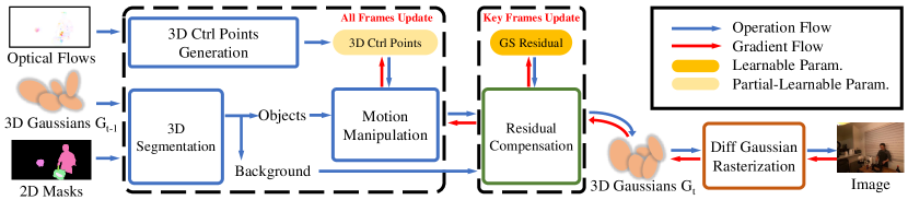
Figure 1: The detailed structure of our workflow begins with segmenting the scene into static background and moving objects, using multiview masks and a Gaussian category voting algorithm. Subsequently, we utilize optical flow to construct a partially learnable system of 3D control points. The motion-related attributes of Gaussians are manipulated on an object-wise basis. Additionally, we update the Gaussian attributes in a key-frame manner to prevent reconstruction failures due to error accumulation. The supplementary scene information for these keyframes is captured as attribute residuals of the Gaussians.

3.1 Overview of Each Module

3D Segmentation. As discussed in Sec. 1, representing local motion discretely can be more efficient than global methods. Nonetheless, defining the regions where this local representation is applicable is essential. We use multiview masks and a Gaussian category voting algorithm to separate the scene into multiple dynamic objects and a static background to achieve this. The control points are specifically designed to influence only those Gaussians categorized as objects.

Object-wise Motion Manipulation. Motion manipulation involves transforming the motion-related attributes of Gaussians from one timestep, $t-1$, to the next, $t$. Manipulating these attributes object-wise ensures that a Gaussian is influenced only by control points that belong to the same category. This selective influence supports the topology changes of spatially adjacent objects and enhances the precision of discrete motion representation.

3D Control Points Generation. This module is pivotal to our workflow. Direct optimization of 3D control points traditionally faces significant challenges due to their high degrees of freedom. To address this, we introduce a local decoupling coordinate system that binds partial parameters of the 3D control points with 2D optical flow. This innovative approach effectively reduces the degrees of freedom for the control points from nine to three, facilitating rapid convergence during optimization.

Residual Compensation. To mitigate error accumulation and ensure stable long-term reconstruction, our workflow incorporates a residual compensation block that operates exclusively at keyframes. Specifically, during non-keyframe intervals, Gaussian attributes are frozen, and updates are confined to the control points. At keyframe junctures, both Gaussian attributes and control points are optimized, allowing comprehensive adjustments that maintain the integrity and continuity of the scene reconstruction.

3.2 Local 6-DoF Motion Decoupling and 3D Control Points Design

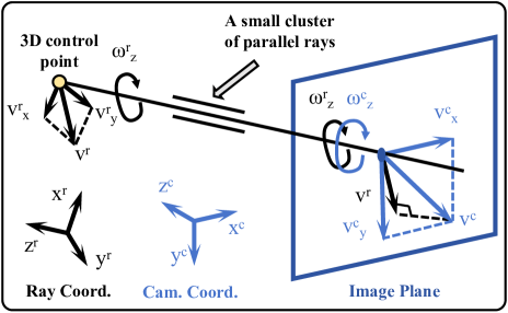
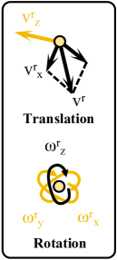
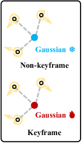
Figure 2: (a) We model the localized light as parallel. The black portions of the 3D control point’s motion parameters, which are carried by parallel rays, are bound with local 2D motion priors derived from the optical flow on the image plane. (b) The yellow segments remain learnable because a small cluster of parallel rays cannot efficiently represent these elements. To facilitate decoupling, rotation attributes are represented in Euler angle format. (c) 3D control points influence their adjacent Gaussian points spatially. During non-keyframe intervals, the attributes of the Gaussians are frozen, and only the learnable parts of the control points are subject to optimization. At keyframes, the attributes of the Gaussians are actively included in the optimization process. For effective interpolation, rotation attributes are expressed in quaternion format.

To discretely represent local 6-degrees-of-freedom (6-DoF) motion, a 3D control point’s attributes must encompass its 3D position, local spatial translation, and local spatial rotation. A portion of local motion is observable from a single viewpoint, expressed as optical flow, while the other is hidden. Hence, we develop a sophisticated local motion decoupling coordinate system, termed the "ray coordinate system," to bind the observable 3D motion components with optical flow from a single viewpoint. Components hidden from this viewpoint are optimized with global image loss as their motion information is implicitly stored across other views.

To simplify the representation of motion, we model a small cluster of localized rays from the scene to the camera as parallel lights. This modeling approach allows the rays to share the same coordinate system, describing the local motion rather than point-wise motion. The justification for this near-parallel hypothesis is detailed in the appendix .1. We establish the z-axis direction of the ray coordinate system to be parallel to the center ray of the cluster, extending from the camera towards the scene. For translation, the component perpendicular to the ray impacts the 2D optical flows observed in the image, while the component along the ray remains invisible. In terms of rotation, a small cluster of parallel rays aligns one rotation component with the normal vector along these rays, equating to translation perpendicular to the rays. The observable rotation appears in the 2D optical flows as a rotation around the cluster center. Conversely, other rotation components, which correspond to translations along these rays, remain undetected in the image plane.

A projection relationship is established between the 2D motion information on the image plane and the motion information carried by parallel light rays. Under the near-parallel hypothesis, points $\mathbf{x}_{i}$ within the neighborhood $\mathcal{N}$ of $\mathbf{x}_{0}$ share the ray coordinate system of $\mathbf{r}_{0}$, as depicted in Fig. 3. Fig. 3 and Eq. 1 detail the translation information $\mathbf{v}_{r}$ carried by rays near the image plane:

$$\mathbf{v}^{r}=f*\frac{1}{N}\sum_{\mathbf{x}_{i}\in\mathcal{N}}(\frac{\mathrm{d}x^{r}_{i}}{\mathrm{d}t},\frac{\mathrm{d}y^{r}_{i}}{\mathrm{d}t})^{\mathrm{T}}=f*\frac{1}{N}\left[\mathbf{R}_{cr}\right]_{:2,:2}\left[\mathbf{K^{-1}}\right]_{:2,:2}\sum_{\mathbf{x}_{i}\in\mathcal{N}}(u_{i},v_{i})^{\mathrm{T}},$$ (1)

where $(u_{i},v_{i})$ represents the optical flow of the points $\mathbf{x}_{i}$. The inverse intrinsic matrix $\mathbf{K^{-1}}$ translates the optical flow from pixel units to base units, and the rotation matrix $\mathbf{R}_{cr}$ transforms the coordinate system from the camera to the ray coordinate system. The notation $\left[\cdot\right]_{:2,:2}$ refers to the matrix’s first and second rows and columns. The variable $N$ denotes the number of pixels in the neighborhood $\mathcal{N}$. The camera’s focal length, $f$, measured in meters, is used to convert the translation from the normalized to the physical image plane, enhancing the interpretability of $\mathbf{v}_{r}$. It is crucial to note that all measurements of $u,v$ are in pixels, while $X,Y,x,y,z$ are expressed in meters.

Next, we back-project the translation information into the scene to obtain the control points’ 3D position and their 2D translation, utilizing the rough depth estimation derived from Gaussian rasterization. Specifically, the critical ratio used in this process is the depth $z^{c}$ relative to the focal length $f$. The formulas for converting the translation and determining the position are presented in Equations 2 and 3, respectively:

$$\mathbf{V}^{r}=(\frac{\mathrm{d}X^{r}}{\mathrm{d}t},\frac{\mathrm{d}Y^{r}}{\mathrm{d}t})^{\mathrm{T}}=\frac{z^{c}}{f}\mathbf{v}^{r},$$ (2)

$$\mathbf{X}^{c}=\frac{z^{c}}{f}(x^{c}_{0},y^{c}_{0},f)^{\mathrm{T}}.$$ (3)

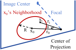
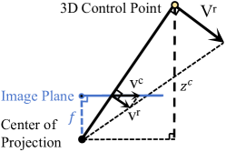
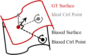
Figure 3: (a) Illustration of angles, points, and rays within the neighborhood of $\mathbf{x}_{0}$. (b) Quantitative illustration of motion projection. (c) Gaussians distributed on the ground truth surface compared to control points situated on a biased surface. The rough depth estimation can lead to biases in the predicted translations stemming from rotational movements

To exploit the motion prior information provided by optical flow, we convert the rotation representation into the Euler angle format to facilitate decoupling. The formulation for angular velocity is specified as follows:

$$\boldsymbol{\omega}^{r}_{z}=\frac{1}{N}\sum_{\mathbf{x}_{i}\in\mathcal{N}}\frac{{(\mathbf{x}^{r}_{i}-\mathbf{x}^{r}_{0})}\times\mathbf{v}^{r}_{i}}{\left\|\mathbf{x}^{r}_{i}-\mathbf{x}^{r}_{0}\right\|^{2}}.$$ (4)

Thus far, the motion decoupling process within the ray coordinate system is completed. We have extracted crucial information, including the 3D position and 2D translation of control points, as well as 1D rotation information from a single viewpoint.

We also explored incorporating local macro rotation, as described in the ED-graph method [42], but observed a performance decline. We hypothesize that this setback stems from the structural differences between Gaussians and meshes; while meshes are tightly clustered on the object surface, Gaussians are distributed more loosely due to their high degrees of freedom. Consequently, we chose to omit the component concerning local macro rotation to minimize biases introduced by rough depth estimations, as illustrated in Fig. 3. This adjustment, though resulting in some sparsity, tailors our motion manipulation method to better suit volumetric radiance representations like Gaussians.

3.3 Object-wise Motion Manipulation

To simplify the mathematical discussion, we treat points and their coordinates interchangeably. For each moving object in the scene, the translation $\mathbf{t}$ and rotation $\mathbf{q}$ of a Gaussian $\mathbf{g}$ are determined by interpolating the translation $\mathbf{t}_{i}$ and rotation $\mathbf{q}_{i}$ of the K-nearest spatially adjacent control points $\mathbf{c}_{i}$ within its neighborhood $\mathcal{N}$. The weights $w_{i}$ for this interpolation are inversely proportional to the Euclidean distance. Importantly, rotations, initially in Euler angle format, are converted to quaternion format to facilitate this interpolation process.

$$(\mathbf{t},\mathbf{q})=\sum_{\mathbf{c}_{i}\in\mathcal{N}}w_{i}*(\mathbf{t}_{i},\mathbf{q}_{i}),$$ (5)

$$w_{i}=\frac{1/\left\|\mathbf{g}-\mathbf{c}_{i}\right\|}{\sum_{\mathbf{c}_{i}\in\mathcal{N}}1/\left\|\mathbf{g}-\mathbf{c}_{i}\right\|}.$$ (6)

3.4 3D Segmentation

A straightforward and efficient method for 3D segmentation is to leverage objects’ 2D masks alongside a statistical approach to categorize Gaussians’ projections from various viewpoints. We utilize the SAM-track method [6] to acquire continuous 2D masks of objects and implement a Gaussian category voting strategy similar to that in SA-GS [11]. However, a key distinction in our approach is the capability to differentiate between multiple objects in the foreground:

$$\begin{gathered}C_{k}=C_{k}+1\quad\text{ if }\mathbf{P}_{j}\mathbf{g}\in\mathbf{m}_{jk},\\ \mathbf{L}=\mathrm{argmax}(\mathbf{C}).\end{gathered}$$ (7)

Specifically, for each Gaussian, there is a unique counter for every object category corresponding to the number of masks. Each Gaussian $\mathbf{g}$ is projected onto the $j^{th}$ image plane. If a Gaussian falls within the boundary of the $k^{th}$ object’s mask, its counter for the $k^{th}$ category is incremented by one. This process is repeated across all training views. After all views have been considered, the label $L$ for each Gaussian is determined based on which category’s counter has the highest count, indicating the category to which the Gaussian belongs.

3.5 Residual Compensation

Our approach utilizes control points to predict 3D motion, but it faces error accumulation over time due to two main factors. First, our scene reconstruction depends on information from previous frames, which might not fully capture areas occluded in earlier observations, like the sides and backs of objects. Second, motion estimation inaccuracies exist between the predicted motion of the Gaussians and the ground truth, particularly evident in Gaussians distant from neighboring control points.

To mitigate error accumulation, we employ a strategy inspired by video coding techniques [54, 44], specifically residual coding. Residual coding in video technology adjusts for discrepancies between original and motion-compensated video frames. Our model uses a keyframe updating method to optimize Gaussians after object-wise motion manipulation, enhancing long-term streaming reconstruction.

As illustrated in Fig.2, in non-keyframes, the attributes of Gaussians are frozen, and only the learnable portion of the 3D control points $\mathbb{C}$ is optimized. The scene at non-keyframe $t$ is represented as follows:

$$\mathbb{G}_{t}=\mathcal{F}_{\mathbb{C}_{t}}(\mathbb{G}_{t-1}),$$ (8)

Where $\mathcal{F}$ denotes object-wise motion manipulation. In keyframes, the attributes of Gaussians are subject to optimization. Gaussian points are not reinitialized; instead, they inherit attributes from previous timestamps. This approach enhances efficiency by updating only the residuals $\mathbb{R}$, which represent minimal deviations. The scene at keyframe $t$ is represented as follows:

$$\mathbb{G}_{t}=\mathcal{F}_{\mathbb{C}_{t}}(\mathbb{G}_{t-1})+\mathbb{R}_{t},$$ (9)

We introduce the concept of Group of Scenes (GoS), analogous to the Group of Pictures (GoP) in video coding.

Specifically, we segment the scene sequence into multiple groups of scenes (GoS), with each group comprising scene information across N consecutive timesteps. Given the initial 3D scene $\mathbb{G}_{0}$ with a GoS-N setting, the model parameters are denoted as follows:

$$\mathbb{G}_{0},\mathbb{C}_{1},\mathbb{C}_{2},\ldots,\mathbb{C}_{N-1},\left(\mathbb{R}_{N},\mathbb{C}_{N}\right),\mathbb{C}_{N+1},\mathbb{C}_{N+2},\ldots$$ (10)

3.6 Loss Function

The loss function is straightforward, as illustrated in Eqn. 11:

$$\begin{gathered}\mathcal{L}=(1-\lambda)\mathcal{L}_{\mathrm{1}}+\lambda\mathcal{L}_{\mathrm{D-SSIM}},\\ \end{gathered}$$ (11)

where $\lambda$ is set to 0.2 as recommended in 3D-GS [16]. Due to the efficiency and robustness of our motion modeling and streaming pipeline, our method converges effectively without the need for additional loss constraints. The inherent design of our system directly specifies the motion of the Gaussians from the structural framework, ensuring accurate and stable convergence.

4 Experiment

4.1 Datasets and Implementation Details

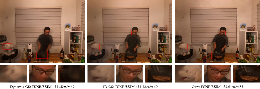
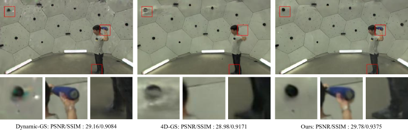
Figure 4: Frame 60 of the "sear_steak" sequence from the Neu3DV dataset [20] and frame 74 of the "softball" sequence from the CMU-Panoptic dataset [15]. We compared our method with Dynamic-GS [28] and 4D-GS [55] across 6 patches. Dynamic-GS provided sub-optimal reconstruction because of the fixed global foreground labels and elaborate regularization terms in the loss function. 4D-GS failed to reconstruct violent motion scenes because of the natural drawback of the global deformation field. In contrast, our method preserves more details and textures, avoiding issues of excessive smoothing and object disappearance.

Neu3DV Dataset [20].

The Neural 3D Video Synthesis Dataset includes six sequences, each originally at a resolution of 2704 $\times$ 2028, but downsampled to 1352 $\times$ 1014 for training. The sequence ’flame_salmon_1’ consists of 1200 frames, whereas the others contain 300 frames each. All sequences are captured by 15 to 20 static cameras, distributed evenly around the scene in a spherical arrangement, with one camera designated for testing and the remainder for training.

CMU-Panoptic Dataset [15].

The CMU-Panoptic Dataset, known for its challenging dynamic object motions, includes three selected sequences. Each sequence has a resolution of 640 $\times$ 360 and spans 150 frames. Captured by 31 static cameras—4 for testing and 27 for training—the cameras are strategically fanned out in front of the scene.

Implementation Details.

Our implementation was based on the Pytorch [33] framework. All trains and tests were conducted on an NVIDIA RTX 4070. We compared our work with methods from Dynamic-GS [28] and 4D-GS [55], which are dynamic reconstruction techniques supporting multiview input using Gaussians. We ran the official codes for these methods, ensuring all approaches shared the same 3D point initialization. Specifically, the 3D points were initialized following the instructions of 4D-GS [55], using COLMAP [36, 37] to process the first frames from all training viewpoints. We further inherited the initial scene’s reconstruction process from dynamic-GS [28], 10k iteration for its training. During training for subsequent frames, we conducted 500 iterations per key frame and 100 iterations per non-key frame. Optimization was performed using a single Adam [17] optimizer with constant learning rates, following the dynamic-GS approach [28]. Adam’s $\beta$ values were set to (0.9,0.999). A Gaussian took its three nearest control points to estimate the motion. In the CMU-Panoptic Dataset, the SAM-track method failed to deal with the condition that objects move in and out of the image. So, we directly reused the foreground mask provided in Dynamic-GS, degrading the motion manipulation from object-wise to the entire foreground level.

Dynamic-GS [28] Setting.

2D foreground masks and initial 3D points’ segmentation labels were required in this approach. We merged our objects’ 2D masks and used the approach proposed in Sec.3.4 to label the initial points, ensuring a fair comparison. We shrank the training iterations from 2k to 0.5k per frame when processing the CMU-Panoptic dataset.

4D-GS [55] Setting.

For the “flame_salmon_1” sequence, four times longer than the other sequences, we expanded the training iterations from 30k to 120k to ensure a fair comparison.

4.2 Reconstruction Results

Table 1: Quantitative results on the Neu3DV dataset.

Scene	sear_steak			cook_spinach			cut_roasted_beef
Metrics	PSNR$\uparrow$	SSIM$\uparrow$	LPIPS$\downarrow$	PSNR$\uparrow$	SSIM$\uparrow$	LPIPS$\downarrow$	PSNR$\uparrow$	SSIM$\uparrow$	LPIPS$\downarrow$
Dynamic-GS	31.38	0.9469	0.1119	29.98	0.9388	0.1179	29.64	0.9360	0.1248
4D-GS	31.62	0.9569	0.0808	32.79	0.9522	0.0926	32.13	0.9467	0.0959
Ours-GoS1	33.23	0.9654	0.0719	33.20	0.9586	0.0796	33.00	0.9609	0.0795
Ours-GoS5	33.72	0.9661	0.0704	32.91	0.9579	0.0819	33.23	0.9592	0.0835
Ours-GoS10	33.64	0.9655	0.0716	32.65	0.9553	0.0861	32.47	0.9555	0.0890
Scene	flame_steak			flame_salmon_1			coffee_martini
Metrics	PSNR$\uparrow$	SSIM$\uparrow$	LPIPS$\downarrow$	PSNR$\uparrow$	SSIM$\uparrow$	LPIPS$\downarrow$	PSNR$\uparrow$	SSIM$\uparrow$	LPIPS$\downarrow$
Dynamic-GS	30.41	0.9429	0.1121	20.19	0.8875	0.1583	24.29	0.8870	0.1630
4D-GS	29.28	0.9545	0.0836	28.27	0.9106	0.1289	28.87	0.9198	0.1168
Ours-GoS1	32.84	0.9645	0.0723	28.00	0.9173	0.1083	26.90	0.9140	0.1170
Ours-GoS5	33.18	0.9649	0.0707	27.65	0.9155	0.1127	26.71	0.9119	0.1242
Ours-GoS10	32.94	0.9631	0.7330	27.17	0.9127	0.1165	26.51	0.9100	0.1283

Table 2: Quantitative results on the CMU-Panoptic dataset.

Scene	softball			boxes			basketball
Metrics	PSNR$\uparrow$	SSIM$\uparrow$	LPIPS$\downarrow$	PSNR$\uparrow$	SSIM$\uparrow$	LPIPS$\downarrow$	PSNR$\uparrow$	SSIM$\uparrow$	LPIPS$\downarrow$
Dynamic-GS	26.93	0.9076	0.1804	27.79	0.9069	0.1769	28.54	0.9032	0.1812
Ours-GoS2	27.48	0.9264	0.1374	27.88	0.9227	0.1413	27.72	0.9203	0.1423

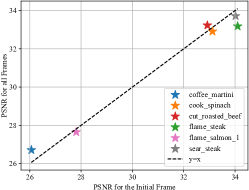
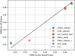
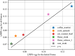
Figure 5: Reconstruction quality correlation between the initial frame and the entire video.

Qualtitative and Subjective Results.

As shown in Tab. 1 and Tab. 2, our approach outperformed dynamic-GS [28] and 4D-GS [55] in most sequences, achieving state-of-the-art (SOTA) performance. 4D-GS’s quantitative results on the CMU-Panoptic dataset were not included because it failed to represent violent scene motion, as shown in Fig. 4. Subjective results further demonstrated that our method preserved more details and provided more robust reconstruction results than previous methods.

Expressiveness of Initial 3D Scene.

The static scene reconstruction quality of the ’coffee_martini’ sequence was poor, which adversely affected the overall 4D reconstruction quality. To evaluate our 4D reconstruction’s dependency on initial 3D models, we analyzed three objective metrics—PSNR, SSIM, and LPIPS-vgg—across individual sequences in the Neu3DV dataset, as shown in Fig.5. We used scatter plots for visualization, with a $y=x$ dashed line indicating equivalent quality between 4D and initial 3D reconstructions. On the one hand, our experiments demonstrate that the video sequence’s reconstruction quality closely aligns with that of the initial frame. On the other hand, no new Gaussians are added throughout the sequence. These two points highlight our method’s efficiency in leveraging the dynamic capabilities of the initial 3D scene.

Covergance Speed.

Our non-keyframes were optimized in less than 2 seconds per frame, whereas keyframes required about 40 seconds each. We anticipate further reductions in processing time as the implementation code is optimized.

4.3 Ablation Study

Sparsification for 3D Control Points.

We illustrated the relationship between the Gaussians and the control points in Fig. 6, where the control points are uniformly distributed on the surfaces of objects. Further sparsification of these control points led to notable gains in compactness with only minimal impact on performance.

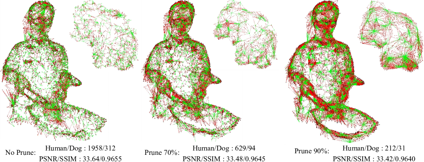
Figure 6: Schematic of Gaussians vs. control points for humans and dogs: We visualized the topology using red and green line segments, with red lines connecting Gaussian points and green lines linking to control points. We also included the number of control points for the first frame of both the human and dog at various pruning rates, alongside the reconstruction quality of the entire sequence.

Points Parameter Comparison.

We detailed a comparison in Tab. 3 of 3D points across different categories to demonstrate the compactness of our control point method. The 13-dimensional attributes of each Gaussian include 3D spherical harmonics, position, rotation, scale, and 1D opacity. The number of parameters for the Gaussians increases as the degree of spherical harmonics increases.

Table 3: Comparison between Gaussians and control points.

Points Category	Points Num.	Attr. Dim.	Param. Num.
Scene Gaussians	$>100k$	$\geq 13$	$>1000k$
Object Gaussians	$\sim 10k$	$\geq 13$	$>100k$
Object Control Points	$0.2k-2.5k$	$3$	$0.6k-7.5k$

Effectiveness of 3D Control Points.

In the GoS-10 configuration, we compared the frame-wise rendering quality of three methods: ’No Control,’ where the scene has no motion manipulation; ’Partial Control,’ using only the projected portion of control points; and ’Full Control,’ which employs both the projected and learned parts of control points. We aligned the Gaussians’ attributes at timesteps 0, 10, and 20 and documented the PSNR metrics for the first 30 frames of the ’sear_steak’ sequence in Fig 7. The observed PSNR gap confirms that integrating both projected and learned control points markedly improves reconstruction results.

3D Motion Visualization.

We visualized the 3D motion of Gaussians in our method. The track precisely described the person turning steaks or getting up to move boxes.

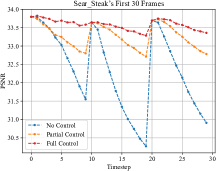
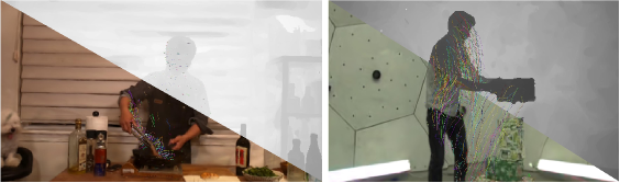
Figure 7: (a) Within each GoS, the reconstruction quality of the "No Control" setup degraded rapidly, the "Partial Control" setup quality degraded moderately, and the "Full Control" setup quality degraded slowly. The keyframe update strategy mitigated error accumulation at timesteps 10 and 20. (b) Visualization for Gaussians’ 3D motion for the “sear_steak” and the “boxes” sequences.

More Advanced Submodule Leads to Better Reconstruction Result.

We investigated the impact of various optical flow methods [43, 19, 35] and determined that DIS [19] achieved the most accurate 2D optical flow predictions for Neu3DV dataset. Optical flow accuracy was quantified by the minimal average MSE between the current frame and its warped predecessor. The lowest 2D errors correlated with superior 3D reconstruction quality, suggesting that our pipeline’s performance could be further improved by incorporating more advanced optical flow predictors. The positive correlation between optical flow accuracy and reconstruction quality also demonstrates the effectiveness of our 3D motion model.

Table 4: Comparison between different optical flow methods.

O.F. Model	Avg. 2D MSE$\downarrow$	Rec. PSNR$\uparrow$	Rec. SSIM$\uparrow$	Rec. LPIPS$\downarrow$
PWC [43]	4.553e-5	33.39	0.9644	0.0737
SpyNet [35]	1.509e-5	33.55	0.9649	0.0725
DIS [19]	1.230e-5	33.64	0.9655	0.0716

5 Conclusion

We introduce a novel discrete 6-DoF motion model that merges traditional graphics with learnable pipelines. This method, which uses partially learnable control points for local 6-DoF motion representation, ensures rapid convergence and robust reconstruction with real-world datasets. Furthermore, we have developed an innovative workflow for streaming 4D real-world reconstruction using Gaussians and control points. Our approach initiates with an initial 3D scene reconstruction and progresses through independent submodules. This modular structure enables future enhancements by optimizing each submodule individually. However, our workflow has its limitations: the quality of 4D reconstruction significantly depends on the initial reconstruction quality, an area we have not fully explored, presenting opportunities for further research. Additionally, our current method does not support monocular videos due to its reliance on multi-view initial frames. We will address these limitations in future work.

Appendix

.1 Near-Parallel Light Hypothesis

In the image plane, a small region with center $\mathbf{x}_{0}$ and the radius $R$ is selected. Then the rays from the projection center connected to each pixel in the region can be regarded as approximate parallel light. We provided a detailed illustration in Fig. 8. For an arbitrary $\mathbf{x}_{i}$ in the $\mathbf{x}_{0}$’s neighborhood, we should prove that the angle $\theta$ between ray $\mathbf{r}_{0}$ and ray $\mathbf{r}_{i}$ is a first-order small quantity.

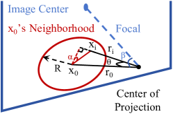
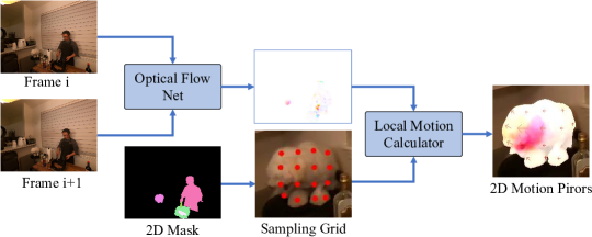
Figure 8: (a) Illustration for angles, points, rays in $\mathbf{x}_{0}$’s neighborhood. (b) Workflow for acquiring 2D motion prior.

First, a plumb line is made from $\mathbf{x}_{0}$ to the ray $\mathbf{r}_{i}$, which is the shortest path from $x_{0}$ to the ray and can be denoted as:

$$\left\|\mathbf{x}_{i}-\mathbf{x}_{0}\right\|\cdot\cos\alpha,$$ (12)

where $\left\|\cdot\right\|$ stands for the Euclidean distance, and $\alpha$ is the angle between the plumb line and line pointing from $\mathbf{x}_{0}$ to $\mathbf{x}_{i}$. Then, using the cosine theorem, the distance from the projection center to $\mathbf{x}_{0}$ can be represented as:

$$f\cdot 1/\cos\beta,$$ (13)

where $f$ is the camera focal length, and $\beta$ is the angle between the ray $\mathbf{r}_{0}$ and the major optical axis. Next, using the sine theorem, $\theta$ can be characterized as :

$$\theta_{i}=\mathbf{arcsin}(\frac{\left\|\mathbf{x}_{i}-\mathbf{x}_{0}\right\|}{f}\cdot\frac{\cos\alpha}{1/\cos\beta}).$$ (14)

The second term is always a real number not greater than 1. Since $\left\|\mathbf{x}_{i}-\mathbf{x}_{0}\right\|$ is always smaller than $R$, $\theta$ remains small if the focal length $f$ is much larger than the neighborhood radius $R$.

Thus far, the proof of Near-parallelism of localized rays is complete. In practice, With a normalized focal length of more than 1000 pixels, it is perfectly acceptable to limit the calculation area to a radius of 50 pixels.

.2 2D Motion Prior Acquisition

We provide an intuitive workflow for the prior acquisition of 3D motion. The inputs consist of two consecutive frames and an object-wise mask.

We first input two consecutive frames into the optical flow network, outputting a whole frame of optical flow. Then, a corresponding sampling grid, based on the objects’ masks, is generated for each object in the view. The local motion calculator is the abstract representation of the method we introduced in Sec. 3.2. The final processed 2D motion prior binds with 3D control points.

Note that 3D control points are obtained from all training viewpoints independently. Thus, the 3D control points collect all the training viewpoint control points. Hence, their distribution is much denser than during single viewpoint control point acquisition, and the range of action of the control points will be smaller. When sampling control points, a larger control point sampling interval should be selected, and for each control point, a smaller range around it should be selected to compute the motion prior.

.3 3D Control Points Prune

Further sparsification of 3D control points can be achieved using clustering methods [18, 39]. Note that 3D control points are obtained from all training viewpoints independently. And there exists no prior knowledge of objects’ geometry and motion. So we aimed for an even distribution of the sparsified control points. We recommended the k-means++ approach [1] due to the large number of clustering centers, which requires a more stable clustering initialization.

.4 More Subjective Results at Novel Viewpoint

We provided more subjective results from different sequences to intuitively evaluate our work. We output the subjective results in the group of two rows, from left to right, top to bottom: GT, Dynamic-GS, 4D-GS, Ours.

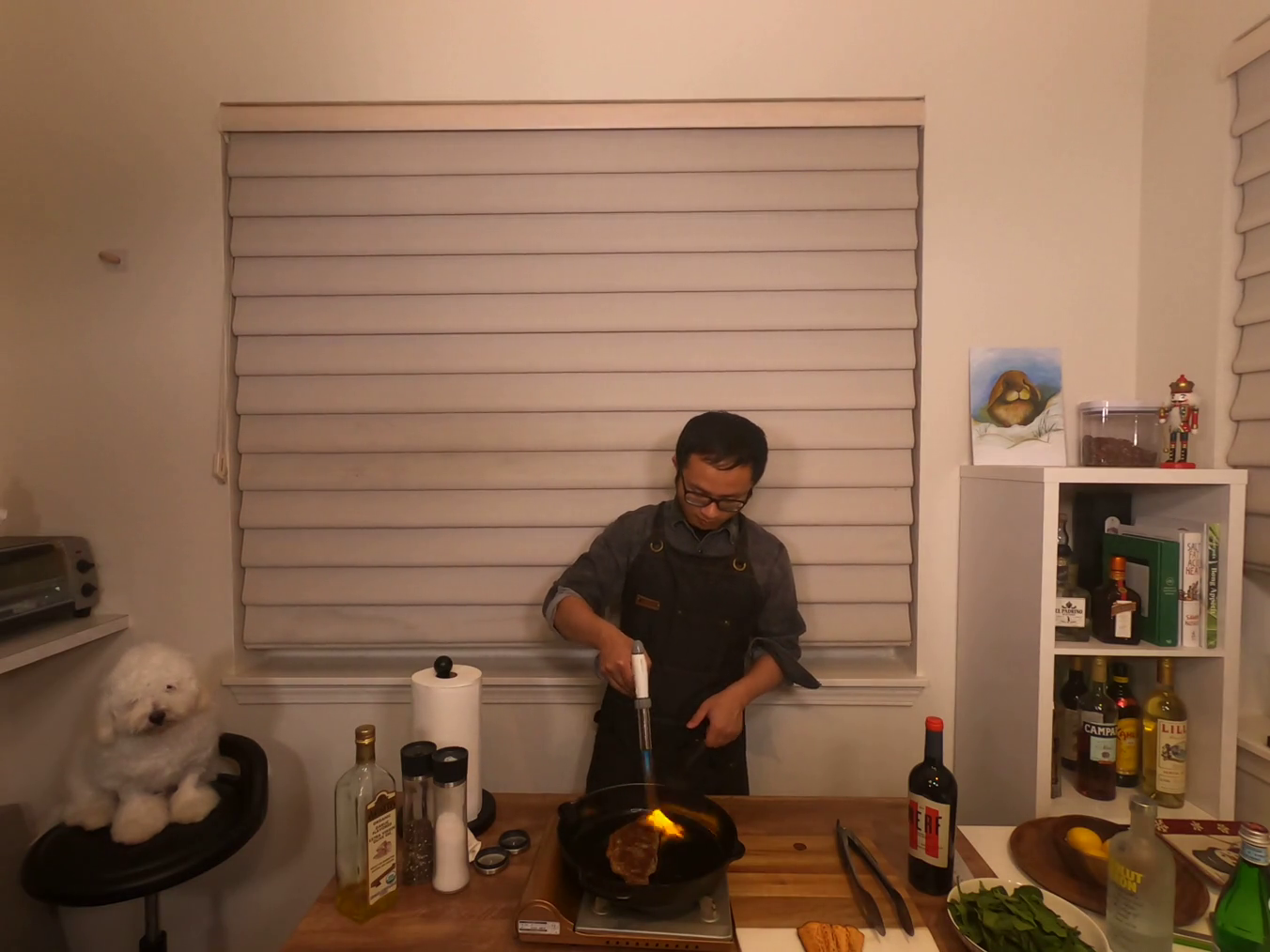
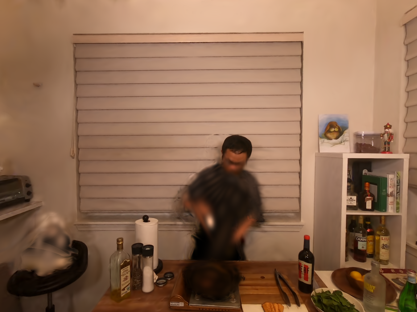
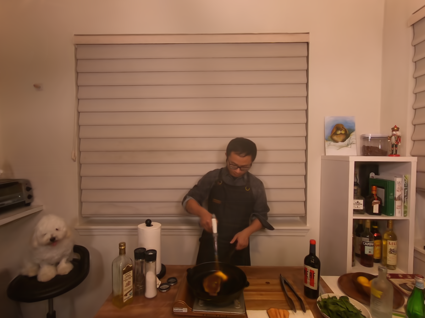
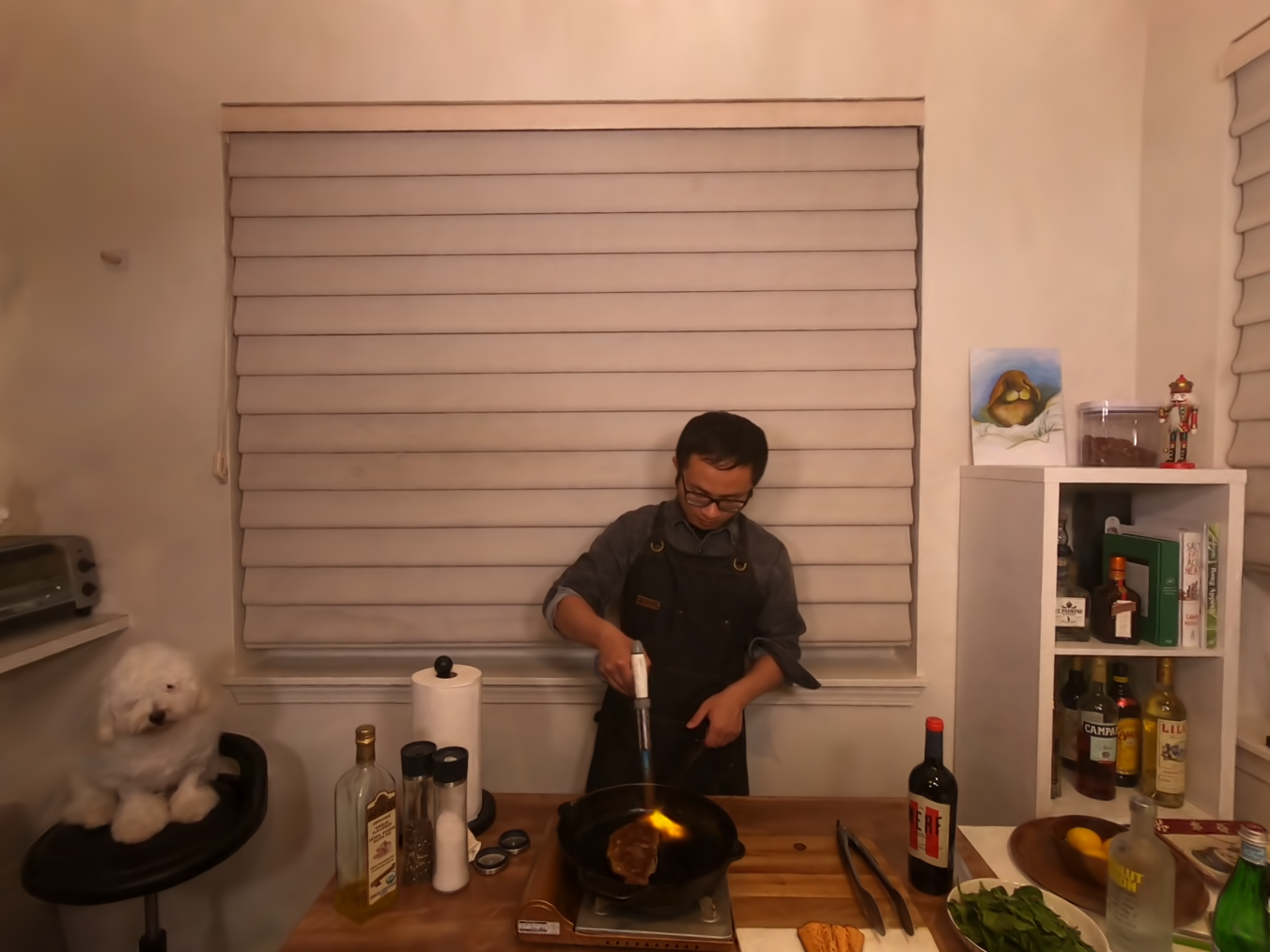
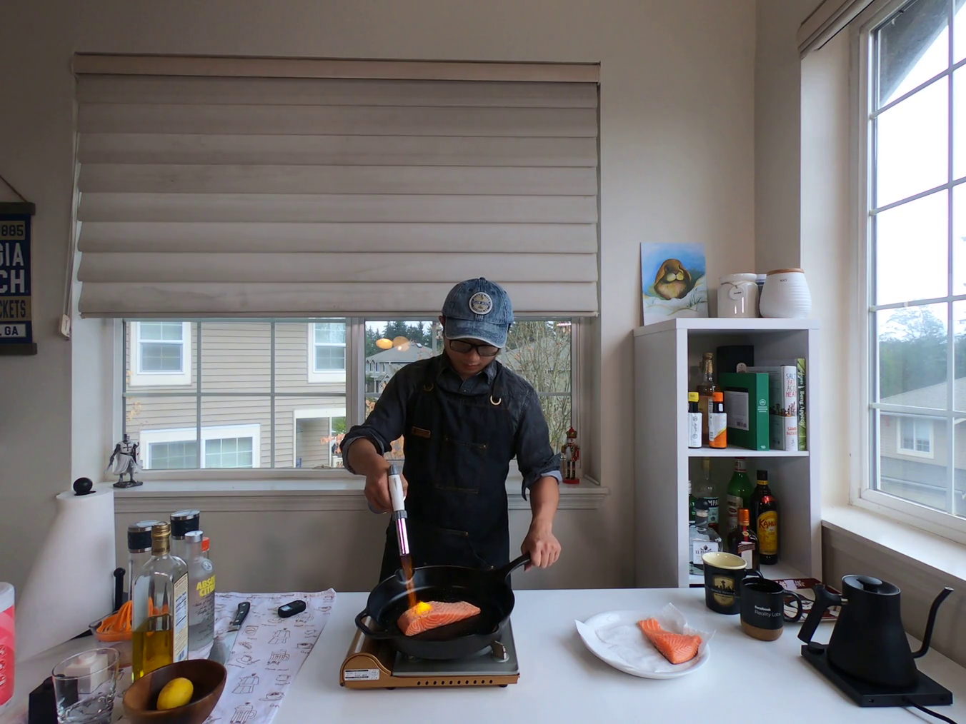
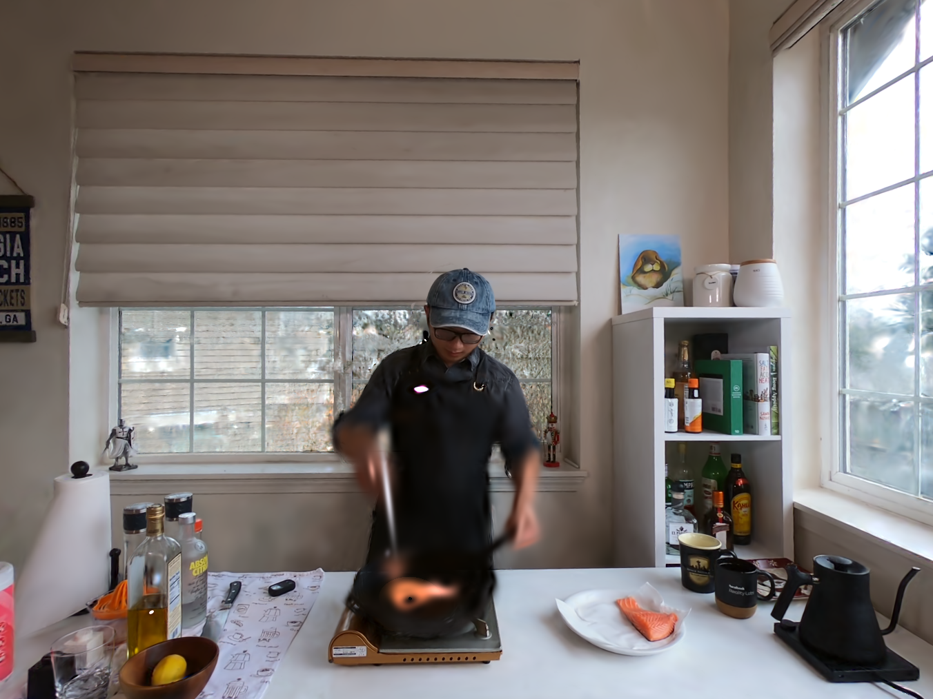
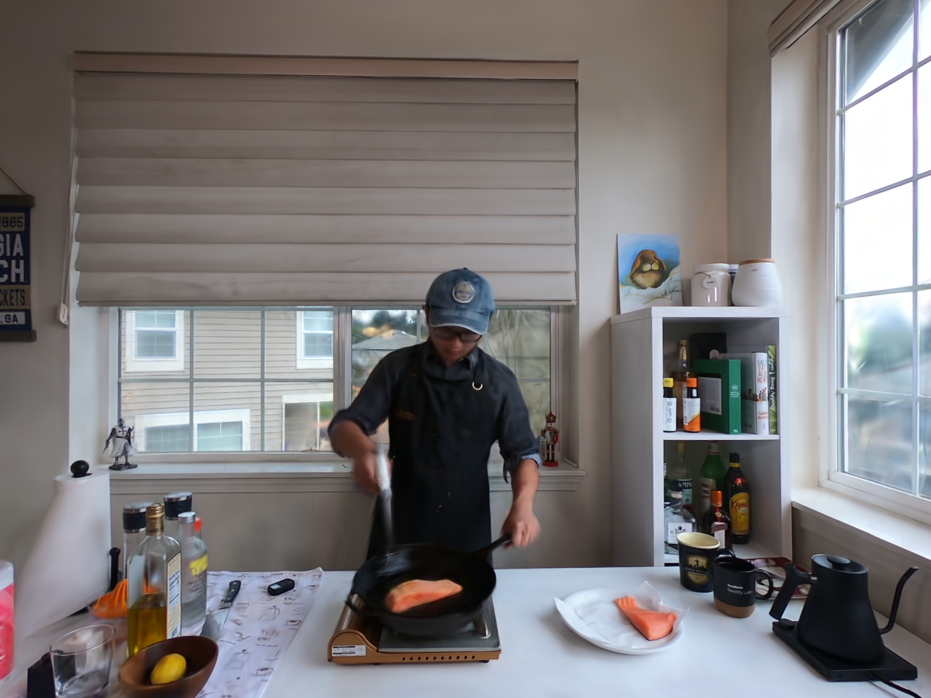
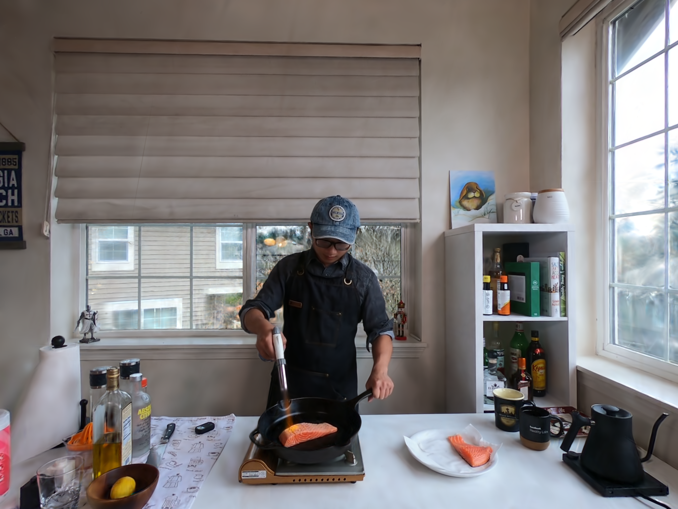
Figure 9: Subjective outputs in groups of two rows, from left to right, top to bottom: Ground truth, Dynamic-GS, 4D-GS, Ours

References

- Arthur et al. [2007] David Arthur, Sergei Vassilvitskii, et al. k-means++: The advantages of careful seeding. In Soda, volume 7, pp. 1027–1035, 2007.
- Attal et al. [2021] Benjamin Attal, Eliot Laidlaw, Aaron Gokaslan, Changil Kim, Christian Richardt, James Tompkin, and Matthew O’Toole. Törf: Time-of-flight radiance fields for dynamic scene view synthesis. Advances in neural information processing systems, 34:26289–26301, 2021.
- Barron et al. [2021] Jonathan T Barron, Ben Mildenhall, Matthew Tancik, Peter Hedman, Ricardo Martin-Brualla, and Pratul P Srinivasan. Mip-nerf: A multiscale representation for anti-aliasing neural radiance fields. In Proceedings of the IEEE/CVF International Conference on Computer Vision, pp. 5855–5864, 2021.
- Barron et al. [2022] Jonathan T Barron, Ben Mildenhall, Dor Verbin, Pratul P Srinivasan, and Peter Hedman. Mip-nerf 360: Unbounded anti-aliased neural radiance fields. In Proceedings of the IEEE/CVF Conference on Computer Vision and Pattern Recognition, pp. 5470–5479, 2022.
- Cao & Johnson [2023] Ang Cao and Justin Johnson. Hexplane: A fast representation for dynamic scenes. In Proceedings of the IEEE/CVF Conference on Computer Vision and Pattern Recognition, pp. 130–141, 2023.
- Cheng et al. [2023] Yangming Cheng, Liulei Li, Yuanyou Xu, Xiaodi Li, Zongxin Yang, Wenguan Wang, and Yi Yang. Segment and track anything. arXiv preprint arXiv:2305.06558, 2023.
- Du et al. [2021] Yilun Du, Yinan Zhang, Hong-Xing Yu, Joshua B Tenenbaum, and Jiajun Wu. Neural radiance flow for 4d view synthesis and video processing. In 2021 IEEE/CVF International Conference on Computer Vision (ICCV), pp. 14304–14314. IEEE Computer Society, 2021.
- Fang et al. [2022] Jiemin Fang, Taoran Yi, Xinggang Wang, Lingxi Xie, Xiaopeng Zhang, Wenyu Liu, Matthias Nießner, and Qi Tian. Fast dynamic radiance fields with time-aware neural voxels. In SIGGRAPH Asia 2022 Conference Papers, pp. 1–9, 2022.
- Fridovich-Keil et al. [2022] Sara Fridovich-Keil, Alex Yu, Matthew Tancik, Qinhong Chen, Benjamin Recht, and Angjoo Kanazawa. Plenoxels: Radiance fields without neural networks. In Proceedings of the IEEE/CVF Conference on Computer Vision and Pattern Recognition, pp. 5501–5510, 2022.
- Fridovich-Keil et al. [2023] Sara Fridovich-Keil, Giacomo Meanti, Frederik Rahbæk Warburg, Benjamin Recht, and Angjoo Kanazawa. K-planes: Explicit radiance fields in space, time, and appearance. In Proceedings of the IEEE/CVF Conference on Computer Vision and Pattern Recognition, pp. 12479–12488, 2023.
- Hu et al. [2024] Xu Hu, Yuxi Wang, Lue Fan, Junsong Fan, Junran Peng, Zhen Lei, Qing Li, and Zhaoxiang Zhang. Semantic anything in 3d gaussians. arXiv preprint arXiv:2401.17857, 2024.
- Huang et al. [2024] Binbin Huang, Zehao Yu, Anpei Chen, Andreas Geiger, and Shenghua Gao. 2d gaussian splatting for geometrically accurate radiance fields. arXiv preprint arXiv:2403.17888, 2024.
- Huang et al. [2023] Yi-Hua Huang, Yang-Tian Sun, Ziyi Yang, Xiaoyang Lyu, Yan-Pei Cao, and Xiaojuan Qi. Sc-gs: Sparse-controlled gaussian splatting for editable dynamic scenes. arXiv preprint arXiv:2312.14937, 2023.
- Jiang et al. [2023] Yuheng Jiang, Zhehao Shen, Penghao Wang, Zhuo Su, Yu Hong, Yingliang Zhang, Jingyi Yu, and Lan Xu. Hifi4g: High-fidelity human performance rendering via compact gaussian splatting. arXiv preprint arXiv:2312.03461, 2023.
- Joo et al. [2017] Hanbyul Joo, Tomas Simon, Xulong Li, Hao Liu, Lei Tan, Lin Gui, Sean Banerjee, Timothy Scott Godisart, Bart Nabbe, Iain Matthews, Takeo Kanade, Shohei Nobuhara, and Yaser Sheikh. Panoptic studio: A massively multiview system for social interaction capture. IEEE Transactions on Pattern Analysis and Machine Intelligence, 2017.
- Kerbl et al. [2023] Bernhard Kerbl, Georgios Kopanas, Thomas Leimkühler, and George Drettakis. 3d gaussian splatting for real-time radiance field rendering. ACM Transactions on Graphics, 42(4):1–14, 2023.
- Kingma & Ba [2014] Diederik P Kingma and Jimmy Ba. Adam: A method for stochastic optimization. arXiv preprint arXiv:1412.6980, 2014.
- Krishna & Murty [1999] K Krishna and M Narasimha Murty. Genetic k-means algorithm. IEEE Transactions on Systems, Man, and Cybernetics, Part B (Cybernetics), 29(3):433–439, 1999.
- Kroeger et al. [2016] Till Kroeger, Radu Timofte, Dengxin Dai, and Luc Van Gool. Fast optical flow using dense inverse search. In Computer Vision–ECCV 2016: 14th European Conference, Amsterdam, The Netherlands, October 11–14, 2016, Proceedings, Part IV 14, pp. 471–488. Springer, 2016.
- Li et al. [2021] Zhengqi Li, Simon Niklaus, Noah Snavely, and Oliver Wang. Neural scene flow fields for space-time view synthesis of dynamic scenes. In Proceedings of the IEEE/CVF Conference on Computer Vision and Pattern Recognition, pp. 6498–6508, 2021.
- Li et al. [2023] Zhengqi Li, Qianqian Wang, Forrester Cole, Richard Tucker, and Noah Snavely. Dynibar: Neural dynamic image-based rendering. In Proceedings of the IEEE/CVF Conference on Computer Vision and Pattern Recognition, pp. 4273–4284, 2023.
- Lin et al. [2022] Haotong Lin, Sida Peng, Zhen Xu, Yunzhi Yan, Qing Shuai, Hujun Bao, and Xiaowei Zhou. Efficient neural radiance fields for interactive free-viewpoint video. In SIGGRAPH Asia 2022 Conference Papers, pp. 1–9, 2022.
- Lin et al. [2023a] Haotong Lin, Sida Peng, Zhen Xu, Tao Xie, Xingyi He, Hujun Bao, and Xiaowei Zhou. Im4d: High-fidelity and real-time novel view synthesis for dynamic scenes. arXiv preprint arXiv:2310.08585, 2023a.
- Lin et al. [2023b] Youtian Lin, Zuozhuo Dai, Siyu Zhu, and Yao Yao. Gaussian-flow: 4d reconstruction with dynamic 3d gaussian particle. arXiv preprint arXiv:2312.03431, 2023b.
- Lin et al. [2024] Youtian Lin, Zuozhuo Dai, Siyu Zhu, and Yao Yao. Gaussian-flow: 4d reconstruction with dynamic 3d gaussian particle. In Proceedings of the IEEE/CVF Conference on Computer Vision and Pattern Recognition, pp. 21136–21145, 2024.
- Liu et al. [2022] Jia-Wei Liu, Yan-Pei Cao, Weijia Mao, Wenqiao Zhang, David Junhao Zhang, Jussi Keppo, Ying Shan, Xiaohu Qie, and Mike Zheng Shou. Devrf: Fast deformable voxel radiance fields for dynamic scenes. Advances in Neural Information Processing Systems, 35:36762–36775, 2022.
- Liu et al. [2023] Yu-Lun Liu, Chen Gao, Andreas Meuleman, Hung-Yu Tseng, Ayush Saraf, Changil Kim, Yung-Yu Chuang, Johannes Kopf, and Jia-Bin Huang. Robust dynamic radiance fields. In Proceedings of the IEEE/CVF Conference on Computer Vision and Pattern Recognition, pp. 13–23, 2023.
- Luiten et al. [2023] Jonathon Luiten, Georgios Kopanas, Bastian Leibe, and Deva Ramanan. Dynamic 3d gaussians: Tracking by persistent dynamic view synthesis. arXiv preprint arXiv:2308.09713, 2023.
- Mildenhall et al. [2021] Ben Mildenhall, Pratul P Srinivasan, Matthew Tancik, Jonathan T Barron, Ravi Ramamoorthi, and Ren Ng. Nerf: Representing scenes as neural radiance fields for view synthesis. Communications of the ACM, 65(1):99–106, 2021.
- Müller et al. [2022] Thomas Müller, Alex Evans, Christoph Schied, and Alexander Keller. Instant neural graphics primitives with a multiresolution hash encoding. ACM transactions on graphics (TOG), 41(4):1–15, 2022.
- Park et al. [2021a] Keunhong Park, Utkarsh Sinha, Jonathan T Barron, Sofien Bouaziz, Dan B Goldman, Steven M Seitz, and Ricardo Martin-Brualla. Nerfies: Deformable neural radiance fields. In Proceedings of the IEEE/CVF International Conference on Computer Vision, pp. 5865–5874, 2021a.
- Park et al. [2021b] Keunhong Park, Utkarsh Sinha, Peter Hedman, Jonathan T Barron, Sofien Bouaziz, Dan B Goldman, Ricardo Martin-Brualla, and Steven M Seitz. Hypernerf: A higher-dimensional representation for topologically varying neural radiance fields. arXiv preprint arXiv:2106.13228, 2021b.
- Paszke et al. [2019] Adam Paszke, Sam Gross, Francisco Massa, Adam Lerer, James Bradbury, Gregory Chanan, Trevor Killeen, Zeming Lin, Natalia Gimelshein, Luca Antiga, et al. Pytorch: An imperative style, high-performance deep learning library. Advances in neural information processing systems, 32, 2019.
- Pumarola et al. [2021] Albert Pumarola, Enric Corona, Gerard Pons-Moll, and Francesc Moreno-Noguer. D-nerf: Neural radiance fields for dynamic scenes. In Proceedings of the IEEE/CVF Conference on Computer Vision and Pattern Recognition, pp. 10318–10327, 2021.
- Ranjan & Black [2017] Anurag Ranjan and Michael J Black. Optical flow estimation using a spatial pyramid network. In Proceedings of the IEEE conference on computer vision and pattern recognition, pp. 4161–4170, 2017.
- Schönberger & Frahm [2016] Johannes Lutz Schönberger and Jan-Michael Frahm. Structure-from-motion revisited. In Conference on Computer Vision and Pattern Recognition (CVPR), 2016.
- Schönberger et al. [2016] Johannes Lutz Schönberger, Enliang Zheng, Marc Pollefeys, and Jan-Michael Frahm. Pixelwise view selection for unstructured multi-view stereo. In European Conference on Computer Vision (ECCV), 2016.
- Shao et al. [2023] Ruizhi Shao, Zerong Zheng, Hanzhang Tu, Boning Liu, Hongwen Zhang, and Yebin Liu. Tensor4d: Efficient neural 4d decomposition for high-fidelity dynamic reconstruction and rendering. In Proceedings of the IEEE/CVF Conference on Computer Vision and Pattern Recognition, pp. 16632–16642, 2023.
- Sinaga & Yang [2020] Kristina P Sinaga and Miin-Shen Yang. Unsupervised k-means clustering algorithm. IEEE access, 8:80716–80727, 2020.
- Song et al. [2023] Liangchen Song, Anpei Chen, Zhong Li, Zhang Chen, Lele Chen, Junsong Yuan, Yi Xu, and Andreas Geiger. Nerfplayer: A streamable dynamic scene representation with decomposed neural radiance fields. IEEE Transactions on Visualization and Computer Graphics, 29(5):2732–2742, 2023.
- Sorkine [2005] Olga Sorkine. Laplacian mesh processing. Eurographics (State of the Art Reports), 4(4):1, 2005.
- Sumner et al. [2007] Robert W Sumner, Johannes Schmid, and Mark Pauly. Embedded deformation for shape manipulation. In ACM siggraph 2007 papers, pp. 80–es. 2007.
- Sun et al. [2018] Deqing Sun, Xiaodong Yang, Ming-Yu Liu, and Jan Kautz. Pwc-net: Cnns for optical flow using pyramid, warping, and cost volume. In Proceedings of the IEEE conference on computer vision and pattern recognition, pp. 8934–8943, 2018.
- Sze et al. [2014] Vivienne Sze, Madhukar Budagavi, and Gary J Sullivan. High efficiency video coding (hevc). In Integrated circuit and systems, algorithms and architectures, volume 39, pp. 40. Springer, 2014.
- Takikawa et al. [2022] Towaki Takikawa, Alex Evans, Jonathan Tremblay, Thomas Müller, Morgan McGuire, Alec Jacobson, and Sanja Fidler. Variable bitrate neural fields. In ACM SIGGRAPH 2022 Conference Proceedings, pp. 1–9, 2022.
- Teed & Deng [2020] Zachary Teed and Jia Deng. Raft: Recurrent all-pairs field transforms for optical flow. In Computer Vision–ECCV 2020: 16th European Conference, Glasgow, UK, August 23–28, 2020, Proceedings, Part II 16, pp. 402–419. Springer, 2020.
- Vedula et al. [1999] Sundar Vedula, Simon Baker, Peter Rander, Robert Collins, and Takeo Kanade. Three-dimensional scene flow. In Proceedings of the Seventh IEEE International Conference on Computer Vision, volume 2, pp. 722–729. IEEE, 1999.
- Wang et al. [2021] Chaoyang Wang, Ben Eckart, Simon Lucey, and Orazio Gallo. Neural trajectory fields for dynamic novel view synthesis. arXiv preprint arXiv:2105.05994, 2021.
- Wang et al. [2023a] Chaoyang Wang, Lachlan Ewen MacDonald, Laszlo A Jeni, and Simon Lucey. Flow supervision for deformable nerf. In Proceedings of the IEEE/CVF Conference on Computer Vision and Pattern Recognition, pp. 21128–21137, 2023a.
- Wang et al. [2023b] Feng Wang, Sinan Tan, Xinghang Li, Zeyue Tian, Yafei Song, and Huaping Liu. Mixed neural voxels for fast multi-view video synthesis. In Proceedings of the IEEE/CVF International Conference on Computer Vision, pp. 19706–19716, 2023b.
- Wang et al. [2022] Liao Wang, Jiakai Zhang, Xinhang Liu, Fuqiang Zhao, Yanshun Zhang, Yingliang Zhang, Minye Wu, Jingyi Yu, and Lan Xu. Fourier plenoctrees for dynamic radiance field rendering in real-time. In Proceedings of the IEEE/CVF Conference on Computer Vision and Pattern Recognition, pp. 13524–13534, 2022.
- Wang et al. [2023c] Peng Wang, Yuan Liu, Zhaoxi Chen, Lingjie Liu, Ziwei Liu, Taku Komura, Christian Theobalt, and Wenping Wang. F2-nerf: Fast neural radiance field training with free camera trajectories. In Proceedings of the IEEE/CVF Conference on Computer Vision and Pattern Recognition, pp. 4150–4159, 2023c.
- Wang et al. [2023d] Yiming Wang, Qin Han, Marc Habermann, Kostas Daniilidis, Christian Theobalt, and Lingjie Liu. Neus2: Fast learning of neural implicit surfaces for multi-view reconstruction. In Proceedings of the IEEE/CVF International Conference on Computer Vision, pp. 3295–3306, 2023d.
- Wiegand et al. [2003] Thomas Wiegand, Gary J Sullivan, Gisle Bjontegaard, and Ajay Luthra. Overview of the h. 264/avc video coding standard. IEEE Transactions on circuits and systems for video technology, 13(7):560–576, 2003.
- Wu et al. [2023] Guanjun Wu, Taoran Yi, Jiemin Fang, Lingxi Xie, Xiaopeng Zhang, Wei Wei, Wenyu Liu, Qi Tian, and Xinggang Wang. 4d gaussian splatting for real-time dynamic scene rendering. arXiv preprint arXiv:2310.08528, 2023.
- Xian et al. [2021] Wenqi Xian, Jia-Bin Huang, Johannes Kopf, and Changil Kim. Space-time neural irradiance fields for free-viewpoint video. In Proceedings of the IEEE/CVF Conference on Computer Vision and Pattern Recognition, pp. 9421–9431, 2021.
- Yang et al. [2023a] Zeyu Yang, Hongye Yang, Zijie Pan, Xiatian Zhu, and Li Zhang. Real-time photorealistic dynamic scene representation and rendering with 4d gaussian splatting. arXiv preprint arXiv:2310.10642, 2023a.
- Yang et al. [2023b] Ziyi Yang, Xinyu Gao, Wen Zhou, Shaohui Jiao, Yuqing Zhang, and Xiaogang Jin. Deformable 3d gaussians for high-fidelity monocular dynamic scene reconstruction. arXiv preprint arXiv:2309.13101, 2023b.
- Yu et al. [2021] Alex Yu, Ruilong Li, Matthew Tancik, Hao Li, Ren Ng, and Angjoo Kanazawa. Plenoctrees for real-time rendering of neural radiance fields. In Proceedings of the IEEE/CVF International Conference on Computer Vision, pp. 5752–5761, 2021.
- Yu et al. [2004] Yizhou Yu, Kun Zhou, Dong Xu, Xiaohan Shi, Hujun Bao, Baining Guo, and Heung-Yeung Shum. Mesh editing with poisson-based gradient field manipulation. In ACM SIGGRAPH 2004 Papers, pp. 644–651. 2004.