The Frame-Dragging effect on the excitation rate of atoms

Abstract

The frame-dragging phenomenon in gravitational fields is revisited to explore the geometric effects induced by spacetime curvature. We quantize a massless scalar field in the spacetime of a rotating sphere, incorporating the frame-dragging frequency into the field modes. The excitation rate for an atom undergoing uniform circular motion and interacting with the scalar field is calculated. Our results reveal that the time-dependent excitation rates of atoms following different trajectories exhibit a common envelope, from which the frame-dragging frequency can be effectively extracted. This discovery leads us to propose a novel detection scheme for measuring the frame-dragging frequency caused by rotating celestial bodies, eliminating the need for traditional starlight calibration methods.

I Introduction

Since the establishment of General Relativity (GR) , its verification has always been an important subject. LIGO have directly detected gravitational waves for the first time, confirming Einstein’s significant prediction about gravitational waves in GR [1]. Besides, there have been experimental programs known as Gravity Probe A and Gravity Probe B. The former aims to test the gravitational redshift effect [2], while the latter is designed to examine the frame-dragging effect [3].However, the two are not equally well-known. Gravity Probe A is more widely recognized, while Gravity Probe B is relatively less known and less frequently discussed.

The studies in this paper consider Gravity Probe B . NASA launched the Gravity Probe B satellite with the goal of verifying Einstein’s GR by detecting the the precession of the gyroscope in curved spacetime. This project is based on a experimental method proposed by L.I. Schiff in 1960 to test GR [4]. Schiff pointed out that a gyroscope orbiting around the rotating Earth would experience precession. This precession is caused by Thomas precession and the frame-dragging effect, the latter of which implies that the local inertial frame around a rotating object would rotate relative to the entire universe. Experimentally, the measurement of the gyroscope’s precession angular velocity is achieved by installing gyroscopic rotors in the satellite and measuring the gyroscope’s deviation relative to a guide star. The experimental detection results for the gyroscope’s drift rate are in agreement with the predicted values from GR. However, the Gravity Probe B experiment (and other experiments with similar objectives [5, 6]) has its limitations. The measurement of the precession angular velocity always requires calibration using the starlight of the guide star (or rely on another reference object), but about 40 percent of the time, the satellite orbiting the Earth is obstructed by the Earth itself, blocking the starlight. Moreover, the starlight itself is not truly stationary due to its own drift and factors like annual parallax. These limitations are inherent in the fact that General Relativity is a classical, local theory, meaning that we can only indirectly determine the relative angular velocity between the local inertial frame and the inertial frame at infinity. However, it is well known that quantum field theory in curved spacetime is a non-local theory, which inspires us to discuss the quantum effects influenced by gravitational frame-dragging.

In quantum field theory in curved spacetime, a well-known result is the Unruh effect (1976) [7], which shows that an atom undergoing uniform acceleration in a vacuum will be excited, and its excitation rate spectrum is equivalent to immersing the atom in a thermal bath. Subsequently, Letaw and Pfautsch (1980) discovered that an atom undergoing uniform circular motion in a vacuum will also be excited, but its excitation rate does not correspond to any thermal spectrum [8]. They also found that the energy level difference $\epsilon_{Max}$, which maximizes the atom’s excitation rate, seems to depend solely on the torsion $\Omega$ of the atom’s world line. Thus, in the case of uniform circular motion, the atom’s excitation rate contains information about the rotational velocity.

In this paper, we aim to understand whether the angular frequency of gravitational frame-dragging can also be reflected in the excitation rate of an atom. It is known that in a Schwarzschild spacetime, an atom at rest would be excited by Hawking radiation due to the mixing of positive and negative frequency modes of the field caused by the presence of the horizon [9]. The excitation rate of the atom contains information about the surface gravity $\kappa$ of the horizon. In Kerr spacetime, there exists a phenomenon known as superradiance, where a rotating black hole scatters incoming waves with frequency $\omega$ lower than $m\Omega_{h}$ to higher energy, losing angular momentum in the process. This process also contains information about the frame-dragging frequency $\Omega_{h}$ at the black hole’s horizon [10, 11, 12, 13, 14]. However, in axisymmetric spacetimes without horizons and singularities, such as the spacetime formed by an ordinary rotating body containing only the exterior solution of the Kerr metric, an atom at rest would not be excited due to the absence of a horizon.

To extract information about the frame-dragging frequency $\Omega$, we note that a rotating reference frame shares many similarities with Kerr spacetime. Therefore, we consider the case of an atom undergoing uniform circular motion in such a spacetime. We first quantize the massless scalar field in a spacetime containing a rotating sphere. We approximate the field modes of the massless scalar field under this metric. These approximations are reasonable, and we show that under these approximations, the internal structure of the sphere no longer needs to be considered, making the discussion broadly applicable to various celestial bodies in the universe. We then discuss the coupling between the quantized scalar field and the atom, considering the case where the atom undergoes uniform circular motion in the locally dragged reference frame, where the atom can be excited. This excitation mechanism is similar to the excitation mechanism of an atom in a rotating coordinate system, as the rotation allows the atom to resonate with the original positive frequency modes of the field. We then calculate the excitation rate of the atom and find that in this case, the excitation rate curves for atoms with different rotational speeds form an envelope with a platform whose height has a simple correspondence with the frame-dragging frequency $\Omega$.

Inspired by this, we further propose a detection scheme that can measure the frame-dragging frequency of the local reference frame through this quantum effect, without relying on stellar calibration.

Unless otherwise stated, we use natural units where $c=\hbar=1$, and the metric signature $(-,+,+,+)$ in this paper.

II QUANTIZATION OF SCALAR FIELDS IN THE SPACETIME OF A ROTATING SPHERE

For a slowly rotating isotropic sphere, the spacetime line element is approximately written as  [15, 16]:

$$ds^{2}=-f(r)dt^{2}+f(r)^{-1}dr^{2}+r^{2}d\theta^{2}+r^{2}\sin^{2}\theta\left(d\phi-\Omega(r)dt\right)^{2}$$ (1)

where $f(r)$ and $\Omega(r)$ are piecewise continuous functions, respectively.

$$f(r)=\begin{cases}1-\frac{2GM}{r}&,r\geq R\\ \textrm{A smooth increasing function}&,0\leq r<R\end{cases}$$ (2)

and

$$\Omega(r)=\begin{cases}\frac{2GJ}{r^{3}}&,r\geq R\\ \textrm{A smooth decreasing function}&,0\leq r<R\end{cases}$$ (3)

Here, $J$ is the angular momentum of the sphere (where the direction of increasing $\phi$ is taken as the positive direction of angular momentum), and $M$ represents the mass of the sphere. Outside the sphere, the spacetime metric is the same as the Kerr metric. Then we assume the sphere is rotating slowly, the Kerr metric in this approximation can be written as a replacement of the Schwarzschild metric $\phi\to\phi-\Omega(r)t$. This means that $\Omega(r)$ physically represents the frame-dragging frequency of spacetime, and the frame-dragging frequency outside the sphere is similar to the magnetic field of a magnetic dipole, which has been widely discussed in gravitomagnetism. Inside the sphere, since we do not know the internal structure of the sphere, we only assume that the metric is continuous and smooth. Thus, we only require that $f(r)$ and $\Omega(r)$ are continuous and smooth inside the sphere and maintain the same trend as the external metric. This requires the former to be an increasing function and the latter to be a decreasing function. As will be discussed later, the specific forms of these two functions do not affect our calculations.

To quantize the massless scalar field $\Psi$ in the above spacetime, we next solve the field equation of the massless scalar field.

$$\frac{1}{\sqrt{-g}}\partial_{\mu}\left(\sqrt{-g}g^{\mu\nu}\partial_{\nu}\Psi\right)=0$$ (4)

where $g$ is the determinant of the metric. Considering that our spacetime is axisymmetric, we may assume that the scalar field $\Psi$ can be separated into variables, i.e.,

$$\Psi_{\omega lm}(t,r,\theta,\phi)=e^{-i\omega t}R_{lm}(r)Y_{lm}(\theta,\phi)$$ (5)

For the metric in Eq.(1) and the field equation in Eq.(4), the radial equation is written as

$$\small\frac{f(r)}{r^{2}}\frac{d}{dr}\left(r^{2}f(r)\frac{d}{dr}R\right)+\left[\left(\omega-m\Omega(r)\right)^{2}-\frac{f(r)l(l+1)}{r^{2}}\right]R=0$$ (6)

We now consider some physical conditions, such as the weak field condition, to appropriately handle the above equation. First, we perform a coordinate transformation $r^{\prime}=r/\sqrt{f(r)}$. In order to simplify Eq.(6), we hope the following approximation condition holds as follow:

$$\frac{d}{dr}\approx\frac{1}{\sqrt{f(r)}}\frac{d}{dr^{\prime}}$$ (7)

This approximation is equivalent to make an assumption $rf^{\prime}(r)\ll 1$. We can estimate $rf^{\prime}(r)$ under weak field conditions. Using the Killing vector field $\xi^{\mu}$ in spacetime, the redshift factor is defined as [17]

$$N=|\xi^{\mu}|=\sqrt{-\xi^{\mu}\xi_{\mu}}$$ (8)

Suppose that an observer moves along the direction of the Killing vector, their acceleration is given by

$$a^{b}=\left(\xi^{a}/N\right)\nabla_{a}\left(\xi^{b}/N\right)$$ (9)

Using the Killing equation $\nabla_{a}\xi_{b}-\nabla_{b}\xi_{a}=0$, the 4-acceleration of the observer’s worldline is expressed as

$$a^{b}=-\nabla^{b}\ln N$$ (10)

In comparison to Newtonian theory, we know that the Newtonian potential $V$ is

$$V=\ln N=\frac{1}{2}\ln\left(-\xi^{a}\xi_{a}\right)$$ (11)

For a slowly rotating sphere, where $\Omega(r)\ll 1$, the redshift factor $N$ is approximated by $\sqrt{f(r)}$. Specifically, in the weak field limit, the function $f(r)$ is expressed in terms of the Newtonian potential $V(r)$ as

$$f(r)=e^{2V(r)}$$ (12)

Without loss of generality, we consider the example of a uniform sphere, for which the Newtonian potential is given by

$$V(r)=\begin{cases}-\frac{GM}{r}&,r\geq R\\ -\frac{3GM}{2R}+\frac{GM}{2R^{3}}r^{2}&,r<R\end{cases}$$ (13)

Based on this, the approximation condition $rf^{\prime}(r)$ is calculated as

$$rf^{\prime}(r)=\begin{cases}\frac{2GM}{r}\left(1-\frac{2GM}{r}\right)&,r\geq R\\ \frac{2GM}{R}e^{-\frac{3GM}{R}}\frac{r^{2}}{R^{2}}e^{\frac{GM}{R}\frac{r^{2}}{R^{2}}}&,r<R\end{cases}$$ (14)

It is easy to see that the weak field condition $GM/r\ll 1$ always ensures that $rf^{\prime}(r)\ll 1$ holds. Therefore, we are effectively assuming a condition weaker than the weak field condition.

Using Eq.(7), the radial equation (6) becomes

$$\frac{d^{2}}{dr^{\prime 2}}R+\frac{2}{r^{\prime}}\frac{d}{dr^{\prime}}R+\left[\left(\omega-m\Omega(r)\right)^{2}-\frac{l(l+1)}{r^{\prime 2}}\right]R=0$$ (15)

We have neglected terms related to $d\sqrt{f(r)}/dr$. This is because we have already assumed $rf^{\prime}(r)\ll 1$, making this term small compared to the term involving $2/r^{\prime}$. Note that Eq.(15) is a spherical Bessel equation with a varying constant. Its first-order solution is a spherical Bessel function $j_{l}(x)$. Higher-order terms involve the first derivative of $\Omega(r)$. Given the slowly rotating condition and the weak field condition we have chosen, only the first-order term is retained. Ultimately, the approximate analytical form of the radial function is obtained as

$$R(r)\approx j_{l}\left(\frac{1}{\sqrt{f(r)}}\left|\omega-m\Omega(r)\right|r\right)$$ (16)

Under the chosen appropriate physical conditions, we find that the approximate expression of the radial function can be obtained without knowing the specific forms of $f(r)$ and $\Omega(r)$, which is beneficial.

Then, we write out the quantized scalar field operator as

$$\hat{\Psi}(t,r,\theta,\phi)=\sum_{|m|\leq l}\int_{0}^{+\infty}d\omega\left(\psi_{\omega lm}e^{-i\omega t}\hat{a}_{\omega lm}+h.c.\right)$$ (17)

where

$$\psi_{\omega lm}=\sqrt{\frac{\omega}{\pi}}Y_{lm}(\theta,\phi)j_{l}\left(\frac{1}{\sqrt{f(r)}}\left|\omega-m\Omega(r)\right|r\right)$$ (18)

is the mode function, $\hat{a}_{\omega lm}$ and $\hat{a}_{\omega lm}^{\dagger}$ are the annihilation and creation operators of the field, respectively, and they satisfy the following commutation relations:

$$\left[\hat{a}_{\omega lm},\hat{a}_{\omega^{\prime}l^{\prime}m^{\prime}}^{\dagger}\right]=\delta_{ll^{\prime}}\delta_{mm^{\prime}}\delta(\omega-\omega^{\prime})$$ (19)

$$\left[\hat{a}_{\omega lm},\hat{a}_{\omega^{\prime}l^{\prime}m^{\prime}}\right]=\left[\hat{a}_{\omega lm}^{\dagger},\hat{a}_{\omega^{\prime}l^{\prime}m^{\prime}}^{\dagger}\right]=0$$ (20)

The coefficient $\sqrt{\omega/\pi}$ in $\psi_{\omega lm}$ arises from normalizing the field modes using the Klein-Gordon inner product.

As expected, since the spacetime in question has no horizon, there is no mode mixing in the field operators. This means that positive norm modes correspond to positive frequency modes, and negative norm modes correspond to negative frequency modes. In the next section, we will see that this implies an atom at rest in the vacuum will not be excited.

It is worth noting that in the aforementioned quantization scheme, we actually considered that the scalar field does not interact directly with the rotating sphere. The interaction between the scalar field and the sphere is only reflected in the fact that the sphere curves spacetime, and the scalar field is influenced by this curved spacetime, with the two interacting indirectly through the background spacetime.

III INTERACTION BETWEEN SCALAR FIELD AND ATOM

III.1 Unruh-DeWitt Detector

Unruh and DeWitt once proposed a detector model to explain why a uniformly accelerated observer would experience a thermal bath [7, 18]. This model can be simplified as follows: consider a two-level atom coupled with a scalar field $\hat{\Psi}$, and the interaction Hamiltonian was written as [19]

$$H_{int}(\tau)=\lambda\left(\sigma^{+}e^{i\epsilon\tau}+\sigma^{-}e^{-i\epsilon\tau}\right)\hat{\Psi}[x^{\mu}(\tau)]$$ (21)

where $\lambda$ is the coupling constant between the atom and the field, $\sigma^{\pm}$ are the raising and lowering operators of the two-level atom, $\epsilon$ represents the energy difference of the atom, $\hat{\Psi}$ is the field operator, and $x^{\mu}(\tau)$ is the trajectory of the atom. The probability amplitude for the system to transition from the vacuum state of the field and the ground state of the atom $|0,g\rangle$ to the $k$-mode of the field and the excited state of the atom $|1_{k},e\rangle$ can be calculated as

$$\begin{split}A_{|0,g\rangle\to|1_{k},e\rangle}&=-i\int_{-\infty}^{+\infty}d\tau\langle 1_{k},e|H_{int}(\tau)|0,g\rangle\\ &=-i\lambda\int_{-\infty}^{+\infty}d\tau e^{i\epsilon\tau}\langle 1_{k}|\widehat{\phi}[x^{\mu}(\tau)]|0\rangle\end{split}$$ (22)

By summing over the modulus squared of the probability amplitude, the probability of the atom transitioning from the ground state to the excited state is obtained as:

$$\small\begin{split}P_{|g\rangle\to|e\rangle}&=\sum_{k}\left|A_{|0,g\rangle\to|1_{k},e\rangle}\right|^{2}\\ &=|\lambda|^{2}\int_{-\infty}^{+\infty}d\tau\int_{-\infty}^{+\infty}d(\Delta\tau)e^{-i\epsilon\Delta\tau}\langle 0|\hat{\Psi}^{\dagger}(\tau+\Delta\tau)\hat{\Psi}(\tau)|0\rangle\\ &=|\lambda|^{2}\int_{-\infty}^{+\infty}d\tau\tilde{G}^{+}(\epsilon)\end{split}$$ (23)

Here, $\tilde{G}^{+}(\epsilon)$ denotes the Fourier transform of the positive frequency Wightman function $G^{+}(\Delta\tau)=\langle 0|\hat{\Psi}^{\dagger}(\tau+\Delta\tau)\hat{\Psi}(\tau)|0\rangle$. It follows from Eq.(23) that the excitation probability per unit proper time is

$$\Gamma^{exc}(\epsilon)=|\lambda|^{2}\tilde{G}^{+}(\epsilon)$$ (24)

For the case where the atom undergoes uniform acceleration with acceleration $a$, it is calculated that $\tilde{G}^{+}(\epsilon)=(\epsilon/2\pi)(\mathrm{e}^{2\pi\epsilon/k_{B}a}-1)^{-1}$, which indicates that the atom will be excited. Furthermore, the excitation rate is the same as that of an atom immersed in a thermal bath at temperature $T=a/2\pi$. This is an interpretation of the Unruh effect.

III.2 Interaction of an Atom with a Scalar Field around a Rotating Sphere

When the time dependence of the field mode $\hat{\Psi}(\tau)$ in Eq.(23) is simply exponential, the excitation rate $\Gamma^{exc}$ of the atom per unit proper time results in the form of Fermi’s golden rule:

$$\Gamma^{exc}(\epsilon)=2\pi|\lambda|^{2}\sum_{n}\left|\psi_{n}\right|^{2}\delta(\epsilon+\omega_{n})$$ (25)

Where we take the Fourier transform of the positive frequency Wightman function $G^{+}(\Delta\tau)$, and $\psi_{n}$ is the time independent mode of $\hat{\Psi}(\tau)$:

$$\hat{\Psi}(\tau)=\sum_{n}\psi_{n}e^{-i\omega_{n}\tau}\hat{a}_{n}+h.c.$$ (26)

It follows from Eq.(25) that when the field operator does not mix frequencies and the atom is at rest, i.e., $\omega_{n}>0$, the factor $\delta(\epsilon+\omega_{n})$ ensures no atom excitation. This situation applies when the atom is at rest in flat spacetime or at rest near a slowly rotating sphere.

A meaningful situation arises when the atom is moving around the sphere. Now, imagine that the atom is performing uniform circular motion near the pole around the rotation axis of the sphere (as shown in Fig.1) with an angular frequency of $\tilde{\Omega}$ (taking the rotation direction of the sphere as positive). Without loss of generality, we assume that the distance from the atom to the center of the sphere is the radius $R$ of the sphere, and the radius of the atom’s motion is $R\sin\theta_{0}$. To obtain the field operator $\hat{\Psi}(\tau)$ experienced by the atom at this time, we take $\phi=\tilde{\Omega}t,\ r=R$, and note that the relationship between the atom’s proper time $\tau$ and the coordinate time $t$ is $d\tau=\sqrt{f(R)-R^{2}\sin^{2}\theta(\tilde{\Omega}-\Omega)^{2}}\,dt\equiv\gamma^{-1}dt$, thus obtaining

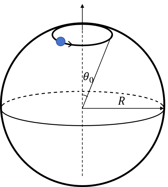
Figure 1: The atom’s trajectory outside the sphere

$$\hat{\Psi}(\tau)=\sum_{|m|\leq l}\int_{0}^{+\infty}d\omega\left(\psi_{\omega lm}^{R}e^{-i(\omega-m\tilde{\Omega})\gamma\tau}\hat{a}_{\omega lm}+h.c.\right)$$ (27)

where

$$\psi_{\omega lm}^{R}=\sqrt{\frac{\omega}{\pi}}Y_{lm}(\theta_{0},0)j_{l}\left(\frac{1}{\sqrt{f(R)}}\left|\omega-m\Omega(R)\right|R\right)$$ (28)

By applying the Fermi’s golden rule (25) here, the excitation rate of the atom is obtained as

$$\begin{split}\Gamma^{exc}(\epsilon)&=2|\lambda|^{2}\sum_{|m|\leq l}\int_{0}^{+\infty}d\omega\omega|Y_{lm}(\theta_{0},0)|^{2}j_{l}^{2}\left(\frac{1}{\sqrt{f(R)}}\left|\omega-m\Omega(R)\right|R\right)\delta\left[\epsilon+(\omega-m\tilde{\Omega})\gamma\right]\\ &=2|\lambda|^{2}\gamma^{-1}\sum_{|m|\leq l}\left(m\tilde{\Omega}-\gamma^{-1}\epsilon\right)\theta\left(m\tilde{\Omega}-\gamma^{-1}\epsilon\right)|Y_{lm}(\theta_{0},0)|^{2}j_{l}^{2}\left(\frac{1}{\sqrt{f(R)}}\left|m(\tilde{\Omega}-\Omega(R))-\gamma^{-1}\epsilon\right|R\right)\end{split}$$ (29)

Here, $\theta\left(m\tilde{\Omega}-\gamma^{-1}\epsilon\right)$ is the Heaviside function, used to filter out the modes that resonate with the atom. Eq.(29) is a function of $\epsilon$ with $\tilde{\Omega}$ as a parameter. We have plotted the atomic excitation rate function $\Gamma^{exc}(\epsilon)$ corresponding to different atomic orbital frequencies $\tilde{\Omega}$ in Fig.2 through numerical calculations. It is noted that an envelope line parameterized by $\tilde{\Omega}$ is formed in Fig.2, represented by a red dashed line. This envelope line is approximately written as

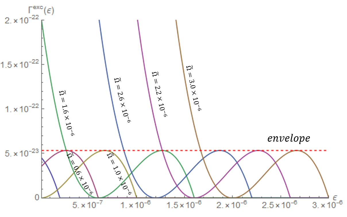
Figure 2: The excitation rate of atoms under different $\tilde{\Omega}$. The dimensionless parameters selected for this figure are $\lambda=1,GM=5\times 10^{-5},\theta_{0}=0.05,\Omega=10^{-6}$. The curves of different colors in the figure form an envelope (red dashed line).

$$\Gamma_{env}^{exc}=\frac{|\lambda|^{2}}{81\pi\sqrt{f(R)}}\Omega^{3}R^{2}\sin^{2}\theta$$ (30)

We set a physical situation $\sqrt{f(R)}\approx 1$, and $R\sin\theta\equiv r_{0}$ is the orbital radius of the atom. Then, Eq.(30) is fully simplified as

$$\Gamma_{env}^{exc}=\frac{|\lambda|^{2}}{81\pi}\Omega^{3}r_{0}^{2}$$ (31)

It is surprising that the non-thermal excitation spectrum of atoms shown in Eq.(29) can have such a simple characteristic associated with the background spacetime.

IV THE QUANTUM DETECTOR OF FRAME-DRAGGING EFFECT

In the previous section, we see that the height of the envelope line has a very simple dependence on the frame-dragging frequency and the orbital radius. Therefore, it can be captured as a useful feature of frame-dragging. Then we designed a detection scheme to measure the frame-dragging frequency caused by celestial bodies.

The basic structure of this detector is the same as discussed in Sec.III.2. As shown in Fig3, a ring of a radius $r_{0}$ rotates in the frame-dragging direction with an angular velocity $\tilde{\Omega}$. Unlike the previous section, we now use a large number of atoms instead of a single atom. This is because the atomic excitation rate calculated in Eq.(29) for single partical is too small to detect. In this regard, we adopt the idea from the Dicke model, utilizing coherent enhancement through a large number of atoms to excite the field [20]. Suppose there exist $N$ atoms placed in a box, where each atom is coupled with the scalar field, and the distance between atoms is sufficiently large so that there is no interaction between atoms. The Hamiltonian for the interaction between such a device and the scalar field read as

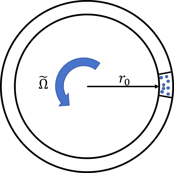
Figure 3: A quantum detector for the frame-dragging effect consists of a ring structure, on which a box filled with atomic gas is mounted, rotating in a circular motion along with the ring.

$$H_{int}(\tau)=\lambda\sum_{i=1}^{N}\left(\sigma_{i}^{+}e^{i\epsilon\tau}+\sigma_{i}^{-}e^{-i\epsilon\tau}\right)\hat{\Psi}(\tau)$$ (32)

To clearly see the relationship between the excitation rate of this system and the number of atoms $N$, we introduce the collective operator of large spin [21]

$$\hat{B}=\frac{1}{\sqrt{N}}\sum_{i=1}^{N}\sigma_{i}^{-},\ \ \hat{B}^{\dagger}=\frac{1}{\sqrt{N}}\sum_{i=1}^{N}\sigma_{i}^{+}$$ (33)

In large $N$ limit, $\hat{B}$ behave as a bosonic operator, with

$$\lim_{N\to+\infty}[\hat{B},\hat{B}^{\dagger}]\to 1.$$ (34)

Therefore, the Hamiltonian in Eq.(32) becomes:

$$H_{int}(\tau)=\sqrt{N}\lambda\left(\hat{B}^{\dagger}e^{i\epsilon\tau}+\hat{B}e^{-i\epsilon\tau}\right)\hat{\Psi}(\tau)$$ (35)

It follows from Eq.(35) that the coupling coefficient $\lambda$ is amplified by a factor of $\sqrt{N}$. Suppose we prepare $N$ particles in the ground state, denoted as $|G\rangle\equiv|g_{1},\cdots,g_{N}\rangle$, and $|1_{B}\rangle\equiv\hat{B}^{\dagger}|G\rangle$. Then the transition rate of the system from $|G\rangle$ to $|1_{B}\rangle$ is essentially the same as that in Eq.(29), with the coupling coefficient $\lambda$ replaced by $\sqrt{N}\lambda$. In other words, the excitation rate is amplified by a factor of $N$. Consequently, for about one mole ($10^{23}$) of atoms, the excitation rate can be increased to a measurable level. By varying the rotating frequency $\tilde{\Omega}$ of the ring, we can obtain the envelope of the excitation rate. Let the height of this envelope be denoted as $\Gamma_{\text{env}}^{\text{exc}}$. Then, the frame-dragging frequency can be inferred from the known parameters of the detector as

$$\Omega=\sqrt[3]{\frac{81\pi\Gamma_{env}^{exc}}{N|\lambda|^{2}r_{0}^{2}}}$$ (36)

Since $N$ is proportional to $\Gamma_{env}^{exc}$, the measured value of $\Omega$ will not be affected by $N$. In some cases, the coupling constant $\lambda$ may be constrained by the particle number $N$, causing $\sqrt{N}\lambda$ to approach a finite value in large $N$ limit.

V CONCLUSION

According to the predictions of General Relativity, a rotating object drags the surrounding spacetime, causing the local inertial frame to exhibit a relative rotational frequency with respect to infinity. In this paper, we have investigated the quantum effects induced by this frame-dragging phenomenon. Our findings demonstrate that the frame-dragging effect generates a distinct excitation rate for atoms undergoing circular motion. Specifically, a group of atoms rotating at different speeds produces a family of excitation rate curves that form an envelope. The height of this envelope is proportional to the cube of the frame-dragging frequency and the square of the radius of motion.

While the thermal spectrum of atoms and its connection to the background spacetime has been well documented, we have shown a specific case where the non-thermal excitation spectrum of atoms can also be directly linked to the background spacetime.

Based on our analysis, we proposed a detection scheme to measure the frame-dragging frequency. This scheme leverages the coherent enhancement resulting from the interaction between a large number of atoms and a scalar field, thereby improving the detection efficiency. Unlike traditional measurement methods, our approach utilizes the non-local properties of quantum field theory, enabling measurements without relying on stellar calibration. Our study offers a novel perspective on investigating the frame-dragging effect.

References

- Abbott et al. [2016] B. P. Abbott, R. Abbott, T. Abbott, M. Abernathy, F. Acernese, K. Ackley, C. Adams, T. Adams, P. Addesso, R. X. Adhikari, et al., Observation of gravitational waves from a binary black hole merger, Physical review letters 116, 061102 (2016).
- Vessot et al. [1980] R. F. Vessot, M. W. Levine, E. M. Mattison, E. Blomberg, T. Hoffman, G. Nystrom, B. Farrel, R. Decher, P. B. Eby, C. Baugher, et al., Test of relativistic gravitation with a space-borne hydrogen maser, Physical Review Letters 45, 2081 (1980).
- Everitt et al. [2011] C. F. Everitt, D. DeBra, B. Parkinson, J. Turneaure, J. Conklin, M. Heifetz, G. Keiser, A. Silbergleit, T. Holmes, J. Kolodziejczak, et al., Gravity probe b: final results of a space experiment to test general relativity, Physical Review Letters 106, 221101 (2011).
- Schiff [1960] L. I. Schiff, Possible new experimental test of general relativity theory, Physical Review Letters 4, 215 (1960).
- Lanzagorta and Salgado [2016] M. Lanzagorta and M. Salgado, Detection of gravitational frame dragging using orbiting qubits, Classical and Quantum Gravity 33, 105013 (2016).
- Di Virgilio et al. [2010] A. Di Virgilio, K. Schreiber, A. Gebauer, J.-P. Wells, A. Tartaglia, J. Belfi, N. Beverini, and A. Ortolan, A laser gyroscope system to detect the gravito-magnetic effect on earth, International Journal of Modern Physics D 19, 2331 (2010).
- Unruh [1976] W. G. Unruh, Notes on black-hole evaporation, Physical Review D 14, 870 (1976).
- Letaw and Pfautsch [1980] J. R. Letaw and J. D. Pfautsch, Quantized scalar field in rotating coordinates, Physical Review D 22, 1345 (1980).
- Hawking [1974] S. W. Hawking, Black hole explosions?, Nature 248, 30 (1974).
- Zel’dovich [1972] Y. B. Zel’dovich, Pis’ ma zh. eksp. teor. fiz. 14, 270 (1971)[jetp lett. 14, 180 (1971)], Zh. Eksp. Teor. Fiz 62, 2076 (1972).
- Misner [1972] C. Misner, Stability of kerr black holes against scalar perturbations, Bulletin of the American Physical Society 17, 472 (1972).
- Ford [1975] L. H. Ford, Quantization of a scalar field in the kerr spacetime, Physical Review D 12, 2963 (1975).
- Unruh [1974] W. G. Unruh, Second quantization in the kerr metric, Physical Review D 10, 3194 (1974).
- Menezes [2017] G. Menezes, Spontaneous excitation of an atom in a kerr spacetime, Physical Review D 95, 065015 (2017).
- Ng et al. [2016] K. K. Ng, R. B. Mann, and E. Martin-Martinez, Equivalence principle and qft: Can a particle detector tell if we live inside a hollow shell?, Physical Review D 94, 104041 (2016).
- Cong et al. [2021] W. Cong, J. Bičák, D. Kubizňák, and R. B. Mann, Quantum detection of inertial frame dragging, Physical Review D 103, 024027 (2021).
- Wald [1984] R. M. Wald, General relativity university of chicago press, chicago 1984, Google Scholar (1984).
- Hawking and Israel [2010] S. Hawking and W. Israel, General relativity: an einstein centenary survey, General relativity: an Einstein centenary survey (2010).
- Crispino et al. [2008] L. C. Crispino, A. Higuchi, and G. E. Matsas, The unruh effect and its applications, Reviews of Modern Physics 80, 787 (2008).
- Dicke [1954] R. H. Dicke, Coherence in spontaneous radiation processes, Physical review 93, 99 (1954).
- Arecchi et al. [1972] F. T. Arecchi, E. Courtens, R. Gilmore, and H. Thomas, Atomic coherent states in quantum optics, Physical Review A 6, 2211 (1972).