Measuring Variable Importance in Individual Treatment Effect Estimation with High Dimensional Data
Abstract
Causal machine learning (ML) promises to provide powerful tools for estimating individual treatment effects. Although causal ML methods are now well established, they still face the significant challenge of interpretability, which is crucial for medical applications. In this work, we propose a new algorithm based on the Conditional Permutation Importance (CPI) method for statistically rigorous variable importance assessment in the context of Conditional Average Treatment Effect (CATE) estimation. Our method termed PermuCATE is agnostic to both the meta-learner and the ML model used. Through theoretical analysis and empirical studies, we show that this approach provides a reliable measure of variable importance and exhibits lower variance compared to the standard Leave-One-Covariate-Out (LOCO) method. We illustrate how this property leads to increased statistical power, which is crucial for the application of explainable ML in small sample sizes or high-dimensional settings. We empirically demonstrate the benefits of our approach in various simulation scenarios, including previously proposed benchmarks as well as more complex settings with high-dimensional and correlated variables that require advanced CATE estimators.
Introduction
The ever growing volume of high-dimensional biomedical data holds promise to facilitate the discovery of novel biomarkers that can predict individual treatment success or risk of adverse events (Pang et al. 2023; Wu et al. 2020; Kong et al. 2022). Transforming complex biological signals into actionable variables, therefore, plays a crucial role for increasing the efficiency of biomedical research and development (Frank and Hargreaves 2003; Hartl et al. 2021). Machine Learning (ML) promises to improve the prediction of biomedical and clinical outcomes from high-dimensional, high-throughput data in various biomedical applications due to its ability to learn complex functions and representations from heterogeneous and correlated data, such as those encountered in e.g. imaging, genomics or transcriptomics data (Le Goallec et al. 2022; Parrish et al. 2024; DeGroat et al. 2023). Regardless, their notorious lack of interpretability hinders the applicability of machine-learning models for generating scientific and clinical insights, motivating efforts for new methods for estimating variable importance within the field of interpretable ML (Molnar 2020; Biecek and Burzykowski 2021). While the results have been promising, most studies have focused on classical ML models like random forests (Strobl et al. 2008), which are well-suited for tabular data with few variables (Grinsztajn, Oyallon, and Varoquaux 2022). A more recent line of work, exposed to complex life-science data, has therefore emphasised the importance of high-capacity ML algorithms and proposed methods combining high-capacity ML algorithms with inference algorithms backed by statistical guarantees. (Mi et al. 2021; Williamson et al. 2023; Lei et al. 2018; Chamma, Thirion, and Engemann 2024).
Despite significant efforts and advances on methods for interpretability, the utility of ML models remains limited as biomedical data are often of interventional nature. Therefore, such datasets are typically analyzed using biostatistical methods appropriate for causal inference and accepted by regulatory agencies. Over the past decade, findings from the causal inference and potential outcomes literature (Imbens and Rubin 2015) have been adapted to propose the estimand framework (Akacha, Bretz, and Ruberg 2017; Ratitch et al. 2020), a flexible statistical-modelling framework useful for analysing clinical data. This development provides formal concepts and notations to separate the quantity of interest from the estimation method. Importantly, this provides a formal language that can bridge the gap between classical biostatistics and ML, hence, pave the way for causal machine learning in biomedical applications (Feuerriegel et al. 2024; Sanchez et al. 2022; Doutreligne and Varoquaux 2023). However, when studying heterogeneity of drug-treatment effects using machine-learning, explainability with statistical guarantees is crucial for uncovering useful predictive biomarkers as ad-hoc methodology may increase the risk of missing important variables or the false positives rate.
Taken together, in the context of present and future biomedical applications, ML methods must address both the complexity of multimodal high-dimensional biological data and support the research questions that arise from interventional studies with estimands such as average treatment effects (ATE) and conditional average treatment effects (CATE). In this context, it is a matter of high priority whether, in the causal setting beyond empirical risk minimization, strategies for variable importance ranking and statistical inference can be applied with intact statistical guarantees.
Contributions. In this work we study algorithms for estimating the importance of variables with statistical guarantees in the context of interventional data and CATE.
- •
-
•
We develop a theoretical analysis of the finite sample variance for both PermuCATE and LOCO, focusing on the impact of estimation error in finite samples.
-
•
Through simulation experiments, we illustrate the differences between these methods in the pre-asymptotic regime, highlighting a larger estimation error for LOCO, which results in higher variance and decreased statistical power.
-
•
We propose a high-dimensional simulation experiment with nonlinear CATE functions to study the scaling behavior of both approaches. This investigation reveals an intensification of the observed trends in more complex scenarios, showing lower variance for PermuCATE.
-
•
Methods are validated using feasible causal risks. Additional analyses show that both PermuCATE and LOCO are insensitive to the choice of feasible causal risk.
The rest of the article unfolds with a review of the related work on variable importance and its rare applications to CATE. The proposed algorithm is then presented and followed by a comparison with the LOCO method on simulation experiments. We finally discuss the implications and limitation of this work.
Related Work
We will now provide an overview of prior art to develop the scientific question addressed by this study. Previous works have analysed (Verdinelli and Wasserman 2023) and benchmarked (Chamma, Engemann, and Thirion 2023) a wealth of procedures and statistical methods for variable importance estimation (Strobl et al. 2008; Liu et al. 2022; Gao et al. 2022; Nguyen, Thirion, and Arlot 2022; Lei et al. 2018; Watson and Wright 2021; Covert, Lundberg, and Lee 2020; Candes et al. 2018; Louppe et al. 2013; Chipman, George, and McCulloch 2010). Out of those approaches, LOCO (Williamson et al. 2023) and CPI (Chamma, Engemann, and Thirion 2023) satisfied the requirements of being model-agnostic (therefore compatible with high-capacity prediction models), offering statistical guarantees for controlling type-1 error, having a realistic computation cost and being interpretable (Chamma, Engemann, and Thirion 2023).
Prior research also studied the problem of variable importance in the case of causal forest estimators (Bénard and Josse 2023) or Bayesian Additive Trees (BART) (Chipman, George, and McCulloch 2010). For biomarker detection in the CATE context, Sechidis, Kormaksson, and Ohlssen (2021) have investigated knock-off procedures with LASSO models and causal forests, which showed good empirical performance on tabular types of medical data but do not offer explicit theoretical guarantees. Moreover, both approaches may encounter intrinsic limits when it comes to high-dimensional data with high correlations and nonlinear functions. Hines, Diaz-Ordaz, and Vansteelandt (2022) have developed a LOCO procedure in concert with the potential-outcomes feasible risk, hence, extending a statistically grounded variable-importance method to the CATE context.
As pointed out by previous work (Chamma, Engemann, and Thirion 2023; Chamma, Thirion, and Engemann 2024), other than permutation methods, LOCO is a refitting procedure requiring a full model fit per variable of interest. The required amount of computation can be expected to be higher in the CATE context, depending on the meta-learner and the choice of feasible risk. It is therefore a question of interest if CPI can be further developed to support variable importance in CATE estimation. Finally a neglected aspect of previous studies of LOCO and CPI is the impact of estimation error that stems from the refitting and the covariate estimation, respectively.
The following sections present a formal treatment of the related work and prepare the ground for our contributions.
Problem setting:
Capital letters denote random variables, and lowercase letters denote their realizations. We consider the potential-outcomes framework with a set of observations . Here, denotes the set of covariates for subject , indicates a binary treatment assignment, and represents the observed outcome. We focus on the estimation of the Conditional Average Treatment Effect , which captures the expected difference between the outcome under treatment () and control () for a subject with covariates . Unlike classical Machine Learning (ML) problems, this function depends on potential outcomes, which are unobserved data since, in general, each subject is assigned to either the treatment or control group. This peculiarity leads to challenges in the estimation procedure of this function as well as in scoring the candidate estimate since the ground truth is not readily available. For a background on CATE estimation and feasible risks, we recommend the work by Kennedy (2023) and by Doutreligne and Varoquaux (2023), respectively.
Leave-One-Covariate-Out (LOCO) for CATE:
Unlike most efforts centered on the estimation of the CATE, in this work, we focus on measuring the importance of the different covariates for CATE prediction. In their work on variable importance for general ML problems, (Williamson et al. 2023) analysed in detail the Leave-One-Covariate-Out (LOCO) approach for estimating the importance of a variable (or group of variables) as the decrease in performance between an estimator fitted on the full set of covariates and the subset of covariates excluding the , that we denote . This approach was then adapted to the causal framework (Hines, Diaz-Ordaz, and Vansteelandt 2022), providing a variable importance measure (VIM) given a risk that measures the predictiveness of a CATE estimator,
| (1) |
where being the CATE estimator fitted on the subset of covariates. In practice, CATE estimators are fitted on a training set, and is evaluated on a disjoint test set.
Feasible Risks for Causal Inference:
The initial formulation of the variable importance measure by Williamson et al. 2023 allows for the choice of different metrics to evaluate the estimator. However, the extension of this framework to causality encounters a fundamental problem in causal inference: the oracle CATE function is not accessible in practice (Holland 1986). Thus, applying ML metrics commonly used for empirical risk minimization in prediction tasks, such as the precision of estimating heterogeneous effects (PEHE), which is the Mean-Squared Error (MSE) in estimating the CATE, is unrealistic. To overcome this hurdle, a feasible risk that can be computed from factual data should be employed to provide practical methods. Hines, Diaz-Ordaz, and Vansteelandt 2022 for instance used the mean squared error between the CATE prediction and the potential-outcome given by
| (2) |
where and denote the response functions: and is the propensity score. Alternatively, a recent review of causal risks (Doutreligne and Varoquaux 2023) for model selection in causal inference suggested using the R-risk given by,
| (3) |
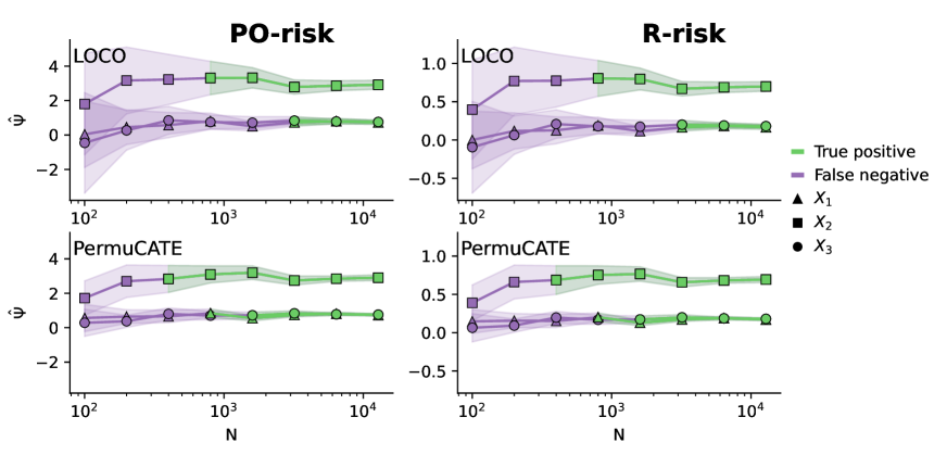
where . This presents greater consistency with the oracle PEHE. We show (cf supplementary materials) that in expectation, both risks can be expressed as a combination of a -MSE and a residual error term weighed by coefficient that involve the propensity score (see supplementary materials). Preliminary experiments presented in the supplementary materials revealed that, for variable importance, both risks yield the same results. Given that the PO-risk is easily comparable to the oracle PEHE, has been used in previous publication and is easy to compute, it is used in the rest of this work.
Conditional Permutation Importance (CPI):
Another line of work on VIM extended this framework by introducing the Conditional Permutation Importance (CPI) measure (Chamma, Engemann, and Thirion 2023). Instead of re-fitting the estimator on a subset of covariates, this method involves shuffling the residual part of a covariate that cannot be inferred from the other covariates. This provides a second estimator of variable importance, denoted described in the case of CATE in equation 4. Similar to LOCO , this approach provides confidence intervals, is model-agnostic, and controls type-1 error. Finally, both approaches present many similarities, among which, in a simplified setup, . A re-scaled therefore leads to values equivalent to the LOCO counterpart.
Computational efficiency:
Other than LOCO, CPI reuses the same estimator when predicting from the perturbed set of covariates. This reduces the computational cost and reduces the error that can be introduced by stochastic optimization of models. It is worth noting that in the work from Hines, Diaz-Ordaz, and Vansteelandt 2022 adapting LOCO for CATE estimation, the full DR-learner is not re-fitted for each covariate subset . Instead, the subset of covariates is projected onto the pseudo-outcomes computed from the full set of covariates . Bypassing the intermediate estimation of the nuisance functions, this trick mitigates the extra computational cost incurred by LOCO when applied to causal estimators as opposed to regular ML problems and avoids violating the unconfoundedness assumption when estimating the CATE with missing covariates. However, in complex scenarios where this final estimation step requires complex models, such as super-learners (Laan, Polley, and Hubbard 2007) or deep neural networks (Curth and Schaar 2021) the computational burden can become intractable.
PermuCATE algorithm
The method presented in this section aims at identifying important variable for CATE prediction. While similarly to LOCO, it is agnostic to the meta-learning approach used to estimated the CATE, we used the DR-learner (Kennedy 2023). This choice is motivated by its favorable convergence properties and the fact that the scoring step requires deriving the pseudo-outcomes, which limits the computational benefits of simpler and more direct meta-learning approaches such as the S- or T-learner.
Input: two independent sets of observations
Parameter: Response functions: ; Propensity: ; CATE: ; Covariate predictor: , feasible risk: , Number of permutations:
Output: Importance estimate
LOCO estimates the importance of a given variable by refitting a model on a subset of covariates, whereas permutation-based approaches reuse the same model to predict from a perturbed design matrix. In the traditional permutation importance approach (Breiman 2001), the perturbed matrix differs from the original by a permutation of the studied covariate. That approach is naive in the sense that it does not account for correlation leading to an increase in type-1 error; CPI, a refined version mitigates this issue (Chamma, Engemann, and Thirion 2023). The key idea is to first predict the covariate (j) from the other covariates, thereby estimating . Then, the residual information can be derived. Afterwards, a perturbed version of the covariate is constructed where is a permutation of the residual. Adapting this idea to the context of CATE estimation allows to obtain, given a causal risk , the following measure of variable importance:
| (4) |
where . PermuCATE (Algorithm 1) describes the procedure to obtain . As suggested in previous work on variable importance, Wald-type statistics can be obtained by using a cross-fitting approach and repeating the algorithm with different data splits (Verdinelli and Wasserman 2023; Chamma, Engemann, and Thirion 2023).
Properties
The following paragraphs compare the properties of the LOCO and PermuCATE estimators in a simplified linear scenario without correlation, to highlight error terms due to finite sample estimations that induce variance. The following section explores experimental results in non-linear scenarios with correlated variables. Previous studies have shown that conditional permutation importance controls for type-1 error and provides statistical guarantees for identifying important variables. Additionally, it can be shown that the importance measured by this method converges to twice the importance measured by the LOCO counterpart. Consequently, defining a re-scaled version of PermuCATE provides an estimator consistent with LOCO, enjoying desirable properties such as linear agreement: in a linear scenario the importance is equal to (Verdinelli and Wasserman 2023). For the remainder of the paper, PermuCATE () will refer to the re-scaled estimator defined in equation (4). A key advantage of this approach is that it allows using an expressive model for the main function estimation, such as a deep neural network, without incurring a heavy cost for refitting the full model, provided a lighter model is used for the covariate prediction. However, in finite sample regimes, this covariate prediction introduces a noise term captured by . In a simplified linear setting (detailed proof in the supplementary materials), when considering a finite training sample and an infinitely large testing sample this estimation error affects the variance of the PermuCATE estimator,
| (5) |
where and are estimated on the finite training set. Similarly, in the LOCO approach, the iterative refitting of the model on the subsets of covariates leads to fluctuations in the estimation of the coefficients . We denote by the difference between the coefficients estimated on the full set of covariates and the coefficient of the model fitted on the subset of covariates. The finite sample variance of the LOCO estimator is then,
| (6) |
It can be seen that in the variance of both estimators converges to the same value, , in the asymptotic case. Moreover, the implied degrees of freedom of the variance terms differ between the two approaches (the norm over a -dimensional vector for LOCO). Consequently, potential difference between the two approaches will only manifest themselves in the finite sample regime.
Therefore, we investigated the variance behavior of both approaches using finite-sample simulations. The results in the following section will show empirically that the error term in LOCO can lead to increased variance and reduced statistical power.
Simulation experiments
Datasets:
This work studies three different simulation scenarios.
-
•
The Low Dimensional (LD) dataset is the data generating process 3 from the work of Hines, Diaz-Ordaz, and Vansteelandt 2022. It is used as a benchmark to compare the proposed approach to their baseline method. It consists of six covariates, each pair being correlated (). Three of these covariates () are linked to the nuisance functions and CATE through linear functions. The analytical importance for these variables is respectively .
-
•
The High Dimensional Linear (HL) dataset is an extension of the work by Doutreligne and Varoquaux 2023 to high dimensional settings. It consists of covariates, 10 of which are linked to the nuisance functions and CATE by a linear function. The loading of each important covariate is drawn from a Rademacher distribution.
-
•
The High Dimensional Polynomial (HP) dataset is similar to HL but uses a linear combination of polynomial features of degree three, including interaction terms.
Further details are provided in the supplementary materials.
Variable importance in low dimensional dataset
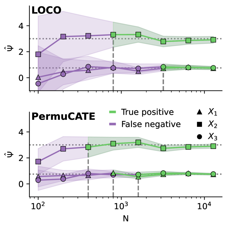
We first compared both approaches using the previously proposed LD benchmark (Hines, Diaz-Ordaz, and Vansteelandt 2022). Out of six covariates, the first three were important for the CATE prediction. To estimate the CATE, we used a DR-learner (Kennedy 2023) with regularized linear models for nuisances functions and the final regression step. For PermuCATE, we used the same regularized linear model for covariate prediction and used 50 permutations. The importance of variables was estimated using a nested cross-fitting scheme. In a first split, of the data was left out for the importance estimation. The remaining was used to fit the DR-learner using the cross-validation scheme presented in the work from Kennedy (2023). We used a five-fold cross-fitting strategy for both loops. Additionally, for each sample size, we repeated these computations on 10 different random samples. The Wald-type statistics where computed over the different folds and random samples by dividing the mean of the distribution by its standard deviation. True positives and false negative were defined with respect to a significance level of . As presented in Figure 1, both methods asymptotically converged to the analytical importance score represented by dotted lines. However, it can be seen that for PermuCATE, the standard deviation was smaller (represented by shaded areas). This larger variance of the LOCO estimator translated into decreased statistical power, as revealed by the minimum sample size needed to identify each of the truly important variables represented by vertical dashed lines.
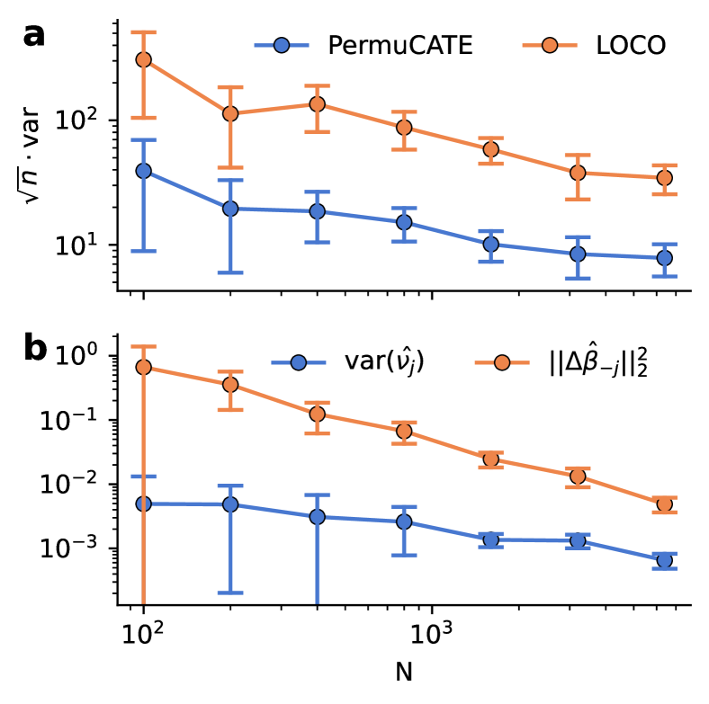
To further investigate the behavior of both methods, we studied how their variance scaled with sample size. Figure 2a represents the variance of both estimators of the importance of the variable , measured over five folds, as a function of sample size. For each sample size, the error bars represent one standard deviation measured over 10 randomly drawn samples. In addition, Figure 2b shows the evolution of the error terms that stem from finite sample fitting. For the LOCO method, as shown in (6), this term corresponds to the variations of the coefficients , while for the CPI approach it corresponds to . Note that to exemplify this behavior, the correlation structure of the LD scenario was removed for this experiment, such that the ground truth was and . This is not the case for correlated scenarios, where non null values of and capture the fact that part of the information of the covariate can be recovered from correlated variables. This second plot reveals that the error term introduced by the refitting in LOCO was orders of magnitude larger than the one introduced by PermuCATE while both converge to the expected value of 0. This was exemplified in this simple linear and low-dimensional scenario. However, as shown in the supplementary materials (Figure 5), the error term becomes even more problematic with growing dimensionality of the problem. The following experiment aimed at studying its impact in more complex and high-dimensional settings.
Variable importance in high dimensional settings
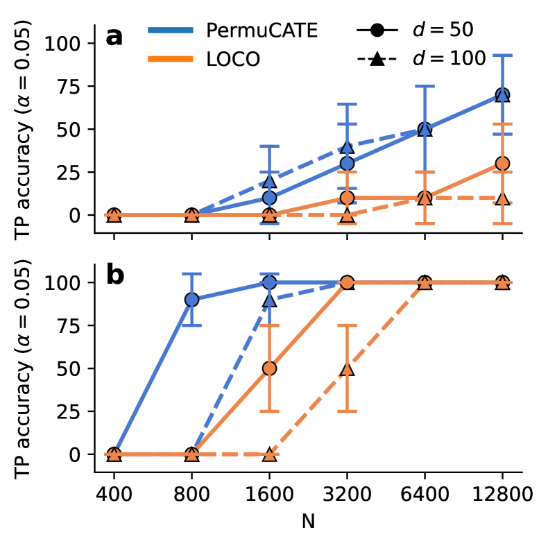
To study the scaling behavior of both methods, we evaluated their capacity to identify important variables in datasets with higher dimensions. We compared their True Positive (TP) accuracy, defined as the proportion of important variables identified as such at a significance level of . We used two simulation scenarios, HL and HP, which respectively use linear and polynomial link functions between the covariates and the different nuisance functions and CATE. For each scenario, two different versions with and covariates were tested. For this more complex setting, the different nuisances and CATE are estimated using a more expressive model, drawing inspiration from the popular Super Learner method (Laan, Polley, and Hubbard 2007). It consists of a stacking of gradient boosting trees and regularize linear model for which a range of hyper-parameters are optimized via cross-validation. All implementations come from scikit-learn (Pedregosa et al. 2011) and additional hyper-parameters are provided in the supplementary materials. Figure 3a presents the TP accuracy, on the HP dataset for different sample size. Besides the superiority of PermuCATE over LOCO for identifying important variables at all sample sizes, it is remarkable that PermuCATE did not suffer from the increase of dimension as opposed to LOCO which identifies less important variable in the case where . This observation likely stems from the fact that the error in scales with the dimension (as shown in Figure 5) while the error term does not. Although not represented on that plot, both methods demonstrated a good control type-1 error. Figure 3b shows the same as (a) but in the linear scenario (HL). Here again, PermuCATE appeared to benefit from increased statistical power, leading to a better identification of important variables in small sample sizes.
Discussion
In this work, we studied two estimators of variable importance in the context of CATE estimation: the LOCO approach (Hines, Diaz-Ordaz, and Vansteelandt 2022) and the proposed PermuCATE algorithm. Our study focused on the pre-asymptotic finite-sample regime, aiming at providing insights on how to select variable importance methods for real-world use cases. The high priority for practical methods also motivated our comparisons of feasible risks for causal methods. Through theoretical analysis and simulation studies covering a wide range of scenarios, we unveiled how noise originating from the finite sample model fitting impacts both algorithms in specific ways through their respective variance terms. We wish to emphasize that this consequential aspect was neglected by most previous work analysing variable importance estimation, which focused more on type-1 error whereas our findings concern type-2 error. Our results imply that the finite-sample-variance behavior could have a critical impact in real-world applications with small- to medium-sized datasets as is characteristic in the biomedical field. For practical applications, we would, thus, recommend PermuCATE over LOCO as both methods enjoys the same statistical guarantees for type-1 error control (as established previously by Chamma, Engemann, and Thirion 2023) while PermuCATE combines shorter computation times with higher power for detecting important variables for predicting treatment success. In the context of exploratory clinical trials in early drug development, this could determine whether informative signals are detected.
Importantly, the present work focused on the application to CATE estimation, however, the theoretical analysis is not limited to the estimation of CATE and also covers variable-importance estimation in the setting of empirical-risk minimization. In other words, we would expect similar results when comparing LOCO algorithm by Williamson et al. (2023) with CPI (Chamma, Engemann, and Thirion 2023) for standard machine-learning problems.
Likewise, this work was motivated to respond to two current trends within the field of life science and health-care research & development: (1) the need for interpretable machine-learning methods for multimodal correlated biomedical data (beyond tabular data and (2) CATE estimation with machine learning in the context of interventional clinical studies for e.g. discovery of predictive biomarkers. While this has shaped the perspective and scope of the present work, it is important to emphasize that the theoretical foundation of our study renders our results general beyond life-science and medical context such as policy-impact, educational or economic applications.
Limitations and future work
The different proofs of the theoretical analysis were limited to a simplified linear case. However, the observations in more complex scenarios, presented in Figure 5 and Figure 3a reveal a similar behaviour as for the linear cases. An extension of the theoretical results to a more general case could therefore be an interesting future contribution.
While the question validating variable importance methods on real-world data is hard in the absence of a known ground truth, previous efforts have focused on semi-synthetic datasets with for instance ACIC 2016 (Dorie et al. 2017) or ACIC 2018 (Shimoni et al. 2018). Such datasets use real covariates and simulated treatment effects and were designed as benchmarks for CATE estimation and not for benchmarks of variable importance estimation within CATE models. As a consequence, the complexity of the function used to simulate the treatment effect is typically provided, but these dataset do not provide the data generating process that would allow to identify the important variables, needed to validate the studied variable importance methods. Having access to this information would allow to benchmark more systematically variable importance methods on established datasets and may foster their development.
It is important to point out that the simulation scenarios studied did not cover extreme correlation (e.g. present in multimodal datasets of medical images and physiological signals) which are known to be problematic, and can potentially lead to both false positives and false negatives. To overcome this hurdle, previous work (Chamma, Thirion, and Engemann 2024) suggested to use block-based approach (i.e. removing or permuting a block of covariates for LOCO or CPI, respectively). We would argue, that in the context of CATE estimation, future work could extend the theoretical analysis and algorithms to cover blocks of correlated variables the same way block-based methods have generalized single-variable methods for standard prediction problems.
Finally, the experiments revealed that LOCO suffers from an increased variance, due to estimation error, when the CATE estimator is a DR-learner using linear models or an adapted version of the super-learner. We argue that this trend should intensify when using more complex CATE estimators, for instance based on neural networks (Curth and Schaar 2021) because of the stochastic optimization, which is an important topic for future research.
References
- Akacha, Bretz, and Ruberg (2017) Akacha, M.; Bretz, F.; and Ruberg, S. 2017. Estimands in clinical trials–broadening the perspective. Statistics in medicine, 36(1): 5–19.
- Biecek and Burzykowski (2021) Biecek, P.; and Burzykowski, T. 2021. Explanatory model analysis: explore, explain, and examine predictive models. Chapman and Hall/CRC.
- Breiman (2001) Breiman, L. 2001. Random forests. Machine learning, 45: 5–32.
- Bénard and Josse (2023) Bénard, C.; and Josse, J. 2023. Variable importance for causal forests: breaking down the heterogeneity of treatment effects. arXiv.
- Candes et al. (2018) Candes, E.; Fan, Y.; Janson, L.; and Lv, J. 2018. Panning for gold:‘model-X’knockoffs for high dimensional controlled variable selection. Journal of the Royal Statistical Society Series B: Statistical Methodology, 80(3): 551–577.
- Chamma, Engemann, and Thirion (2023) Chamma, A.; Engemann, D. A.; and Thirion, B. 2023. Statistically Valid Variable Importance Assessment through Conditional Permutations. Advances in Neural Information Processing Systems.
- Chamma, Thirion, and Engemann (2024) Chamma, A.; Thirion, B.; and Engemann, D. 2024. Variable importance in high-dimensional settings requires grouping. In Proceedings of the AAAI Conference on Artificial Intelligence, volume 38, 11195–11203.
- Chipman, George, and McCulloch (2010) Chipman, H. A.; George, E. I.; and McCulloch, R. E. 2010. BART: Bayesian additive regression trees.
- Covert, Lundberg, and Lee (2020) Covert, I.; Lundberg, S. M.; and Lee, S.-I. 2020. Understanding global feature contributions with additive importance measures. Advances in Neural Information Processing Systems, 33: 17212–17223.
- Curth and Schaar (2021) Curth, A.; and Schaar, M. v. d. 2021. Nonparametric Estimation of Heterogeneous Treatment Effects: From Theory to Learning Algorithms. Advances in Neural Information Processing Systems.
- DeGroat et al. (2023) DeGroat, W.; Mendhe, D.; Bhusari, A.; Abdelhalim, H.; Zeeshan, S.; and Ahmed, Z. 2023. IntelliGenes: a novel machine learning pipeline for biomarker discovery and predictive analysis using multi-genomic profiles. Bioinformatics, 39(12): btad755.
- Dorie et al. (2017) Dorie, V.; Hill, J.; Shalit, U.; Scott, M.; and Cervone, D. 2017. Automated versus do-it-yourself methods for causal inference: Lessons learned from a data analysis competition. arXiv.
- Doutreligne and Varoquaux (2023) Doutreligne, M.; and Varoquaux, G. 2023. How to select predictive models for causal inference? arXiv.
- Feuerriegel et al. (2024) Feuerriegel, S.; Frauen, D.; Melnychuk, V.; Schweisthal, J.; Hess, K.; Curth, A.; Bauer, S.; Kilbertus, N.; Kohane, I. S.; and van der Schaar, M. 2024. Causal machine learning for predicting treatment outcomes. Nature Medicine, 30(4): 958–968.
- Frank and Hargreaves (2003) Frank, R.; and Hargreaves, R. 2003. Clinical biomarkers in drug discovery and development. Nature reviews Drug discovery, 2(7): 566–580.
- Gao et al. (2022) Gao, Y.; Stevens, A.; Raskutti, G.; and Willett, R. 2022. Lazy Estimation of Variable Importance for Large Neural Networks. In International Conference on Machine Learning, 7122–7143. PMLR.
- Grinsztajn, Oyallon, and Varoquaux (2022) Grinsztajn, L.; Oyallon, E.; and Varoquaux, G. 2022. Why do tree-based models still outperform deep learning on typical tabular data? Advances in neural information processing systems, 35: 507–520.
- Hartl et al. (2021) Hartl, D.; de Luca, V.; Kostikova, A.; Laramie, J.; Kennedy, S.; Ferrero, E.; Siegel, R.; Fink, M.; Ahmed, S.; Millholland, J.; et al. 2021. Translational precision medicine: an industry perspective. Journal of translational medicine, 19(1): 245.
- Hines, Diaz-Ordaz, and Vansteelandt (2022) Hines, O.; Diaz-Ordaz, K.; and Vansteelandt, S. 2022. Variable importance measures for heterogeneous causal effects. arXiv.
- Holland (1986) Holland, P. W. 1986. Statistics and Causal Inference. Journal of the American Statistical Association, 81(396): 945.
- Imbens and Rubin (2015) Imbens, G. W.; and Rubin, D. B. 2015. Causal inference in statistics, social, and biomedical sciences. Cambridge university press.
- Kennedy (2023) Kennedy, E. H. 2023. Towards optimal doubly robust estimation of heterogeneous causal effects. Electronic Journal of Statistics.
- Kong et al. (2022) Kong, J.; Ha, D.; Lee, J.; Kim, I.; Park, M.; Im, S.-H.; Shin, K.; and Kim, S. 2022. Network-based machine learning approach to predict immunotherapy response in cancer patients. Nature communications, 13(1): 3703.
- Laan, Polley, and Hubbard (2007) Laan, M. J. v. d.; Polley, E. C.; and Hubbard, A. E. 2007. Super Learner. Statistical Applications in Genetics and Molecular Biology.
- Le Goallec et al. (2022) Le Goallec, A.; Diai, S.; Collin, S.; Prost, J.-B.; Vincent, T.; and Patel, C. J. 2022. Using deep learning to predict abdominal age from liver and pancreas magnetic resonance images. Nature Communications, 13(1): 1979.
- Lei et al. (2018) Lei, J.; G’Sell, M.; Rinaldo, A.; Tibshirani, R. J.; and Wasserman, L. 2018. Distribution-free predictive inference for regression. Journal of the American Statistical Association, 113(523): 1094–1111.
- Liu et al. (2022) Liu, M.; Katsevich, E.; Janson, L.; and Ramdas, A. 2022. Fast and powerful conditional randomization testing via distillation. Biometrika, 109(2): 277–293.
- Louppe et al. (2013) Louppe, G.; Wehenkel, L.; Sutera, A.; and Geurts, P. 2013. Understanding variable importances in forests of randomized trees. Advances in neural information processing systems, 26.
- Mi et al. (2021) Mi, X.; Zou, B.; Zou, F.; and Hu, J. 2021. Permutation-based identification of important biomarkers for complex diseases via machine learning models. Nature communications, 12(1): 3008.
- Molnar (2020) Molnar, C. 2020. Interpretable machine learning. Lulu. com.
- Nguyen, Thirion, and Arlot (2022) Nguyen, B. T.; Thirion, B.; and Arlot, S. 2022. A conditional randomization test for sparse logistic regression in high-dimension. Advances in Neural Information Processing Systems, 35: 13691–13703.
- Pang et al. (2023) Pang, M.; Gabelle, A.; Saha‐Chaudhuri, P.; Huijbers, W.; Gafson, A.; Matthews, P. M.; Tian, L.; Rubino, I.; Hughes, R.; Moor, C. d.; Belachew, S.; and Shen, C. 2023. Precision medicine analysis of heterogeneity in individual‐level treatment response to amyloid beta removal in early Alzheimer’s disease. Alzheimer’s & Dementia.
- Parrish et al. (2024) Parrish, R. L.; Buchman, A. S.; Tasaki, S.; Wang, Y.; Avey, D.; Xu, J.; De Jager, P. L.; Bennett, D. A.; Epstein, M. P.; and Yang, J. 2024. SR-TWAS: leveraging multiple reference panels to improve transcriptome-wide association study power by ensemble machine learning. Nature Communications, 15(1): 6646.
- Pedregosa et al. (2011) Pedregosa, F.; Varoquaux, G.; Gramfort, A.; Michel, V.; Thirion, B.; Grisel, O.; Blondel, M.; Prettenhofer, P.; Weiss, R.; Dubourg, V.; Vanderplas, J.; Passos, A.; Cournapeau, D.; Brucher, M.; Perrot, M.; and Duchesnay, E. 2011. Scikit-learn: Machine Learning in Python. Journal of Machine Learning Research, 12: 2825–2830.
- Ratitch et al. (2020) Ratitch, B.; Bell, J.; Mallinckrodt, C.; Bartlett, J. W.; Goel, N.; Molenberghs, G.; O’Kelly, M.; Singh, P.; and Lipkovich, I. 2020. Choosing estimands in clinical trials: putting the ICH E9 (R1) into practice. Therapeutic innovation & regulatory science, 54: 324–341.
- Sanchez et al. (2022) Sanchez, P.; Voisey, J. P.; Xia, T.; Watson, H. I.; O’Neil, A. Q.; and Tsaftaris, S. A. 2022. Causal machine learning for healthcare and precision medicine. Royal Society Open Science, 9(8): 220638.
- Sechidis, Kormaksson, and Ohlssen (2021) Sechidis, K.; Kormaksson, M.; and Ohlssen, D. 2021. Using knockoffs for controlled predictive biomarker identification. Statistics in Medicine, 40(25): 5453–5473.
- Shimoni et al. (2018) Shimoni, Y.; Yanover, C.; Karavani, E.; and Goldschmnidt, Y. 2018. Benchmarking Framework for Performance-Evaluation of Causal Inference Analysis. arXiv.
- Strobl et al. (2008) Strobl, C.; Boulesteix, A.-L.; Kneib, T.; Augustin, T.; and Zeileis, A. 2008. Conditional variable importance for random forests. BMC bioinformatics, 9: 1–11.
- Verdinelli and Wasserman (2023) Verdinelli, I.; and Wasserman, L. 2023. Feature Importance: A Closer Look at Shapley Values and LOCO. arXiv.
- Watson and Wright (2021) Watson, D. S.; and Wright, M. N. 2021. Testing conditional independence in supervised learning algorithms. Machine Learning, 110(8): 2107–2129.
- Williamson et al. (2023) Williamson, B. D.; Gilbert, P. B.; Simon, N. R.; and Carone, M. 2023. A General Framework for Inference on Algorithm-Agnostic Variable Importance. Journal of the American Statistical Association.
- Wu et al. (2020) Wu, W.; Zhang, Y.; Jiang, J.; Lucas, M. V.; Fonzo, G. A.; Rolle, C. E.; Cooper, C.; Chin-Fatt, C.; Krepel, N.; Cornelssen, C. A.; et al. 2020. An electroencephalographic signature predicts antidepressant response in major depression. Nature biotechnology, 38(4): 439–447.
Supplementary Materials
Notations
| Covariates | |
| Treatment assignment | |
| Outcome | |
| Control response | |
| Treatment response | |
| Conditional Average Treatment Effect | |
| Propensity score | |
| Finite sample estimate of a function | |
| Set of covariates excluding covariate | |
| , Finite sample estimate of covariate from other | |
| , Residual of covariate that cannot be predicted from the others | |
| , Permuted version of the residual | |
| dimensional vector containing as entries, for , where are the coefficients of the | |
| model fitted on the full set of covariates and are the coefficients of the model fitted on the subset of covariates |
R- and pseudo-outcome-risk decomposition
In a scenario where the outcome is not deterministic: , given a CATE estimate , the expectation of the pseudo-outcome risk can be formulated as,
| (S1) |
Similarly, as shown in Doutreligne and Varoquaux 2023, , the R-risk can be re-written as,
| (S2) |
Both risks are therefore comparable in the sense that they are feasible when estimated values are used for the quantities and that they involve a combination of a -MSE and a noise term (termed Bayes error in Doutreligne and Varoquaux 2023). However, the presence of the term at the denominator in S1 makes the quantity less stable and thus desirable for CATE estimator selection. For instance, in a scenario where the propensity score is poorly fitted and can take extreme values (close to or ) a DR-learner might still provide reliable estimation of the CATE. However, the term will likely take extreme values and lead to inconsistencies between the -risk and the oracle -MSE. While this consideration holds for model selection of CATE estimators and is consistent with the findings from Doutreligne and Varoquaux 2023, as shown in 4 we did not notice any difference for the estimation of variable importance. It is likely that noise terms cancel when taking the difference in the variable importance for either LOCO or CPI. The following figure depicts the comparable experimental results up to a scaling factor for the scenario LD
Finite sample estimation of LOCO and CPI
This analysis focuses on the behavior of CPI and LOCO in the finite training sample regime. We therefore assume that is fixed which induces estimation error for the different estimators. However, we often look at the asymptotic when which removes the randomness that stems from the covariates on the testing set.
We consider the case of a linear relationship between the outcome and a set of covariates: where . We denote the function (here a linear model) estimated on a training set of samples and the function fitted on the subset of covariates . We denote by the difference between the coefficients of the linear model fitted on the full set of covariate and the coefficients obtained after fitting on the subset of covariates . In the following notation we omit the sample index in the sum for readability. These indices would affect the covariates , for CPI the covariate prediction and the residual
| (1) |
In the absence of correlation, if we assume the covariates to be normal variables, we obtain . If we additionally look at the asymptotic in , the estimation error has a limit and we get . In the presence of correlation, the re-fitting will attribute an increased loading to variables correlated with and the terms involving will lower the importance.
Regarding CPI, we denote by the estimation of the covariate given the rest of the covariates fitted on the training set.
Here, in the absence of correlation, and if its estimate is unbiased and . Consequently, and Consequently, using a re-scaled estimators provides an estimator consistent with .
Variance of the estimators
We first consider a case where covariates are uncorrelated. In that case . Here again, summation indices are omitted for readability.
From line 2 to 3, several terms that have a null expectation on the test set are omitted, knowing that the expectation on the test set and that covariates are uncorrelated.
From line 2 to 3 several terms that have a null expectation are omitted, knowing that For the variance as well, we see that in the asymptotic in , when the estimation error disappear, the re-scaled version of CPI has a variance consistent with the LOCO approach: var() = var() = var() = var()
Finite sample fitting error for LOCO in high dimension
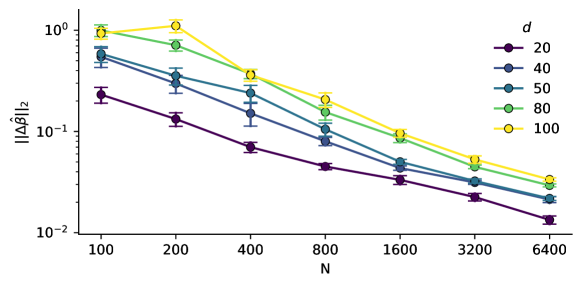
Similarly to Figure 2 we study the estimation error term in LOCO, as a function of the sample size . In this experiment, we however consider the dataset HL and look at different values of the dimension: . This result reveals that the refitting error term grows with the dimension. This trend is associated with an increase in variance that affects the statistical power of LOCO. Note that LOCO also suffers from computation time issues in such settings. Indeed, the method requires refitting the full model times. While this is feasible for simple linear models in that case, it becomes intractable for more complex ones.
Datasets
Low Dimensional (LD) dataset
Taken from the work of Hines, Diaz-Ordaz, and Vansteelandt 2022:
The High Dimensional Linear (HL) dataset
Create the sets of important variables, respectively for the functions by randomly drawing without replacement important variables from the set of possible variables. We denote the vector of covariates . Covariates follow a random normal distribution and with a correlation coefficient that can be modified.
| A Rademacher variable takes value in with equal probability. |
We then construct,
Where denotes the effect size which controls the strength of the treatment effect.
The High Dimensional Polynomial (HL) dataset
This dataset has a similar construction as HL but uses polynomial features. Consequently,
and follow a similar construction as in LD using the same polynomial features.
In addition, we also control the proportion of treated units by computing the quantile of the propensity scores that we denote in order to avoid extreme imbalances between the number of units in the treated and control group.
Hyper-parameter search
For linear models, we used the scikit learn implementation RidgeCV for regression and LogisticRegressionCV with a range of penalization strength from to with 10 logarithmically spaced values. For the gradient boosting tree we used the implementations HistGradientBoostingClassifier and HistGradientBoostingRegressor respectively for regression and classification. After using a randomized search for hyper-parameters we used a learning rate of (range explored: ) and a maximum number of leaves for each tree of (range explored: ).