Air-HOLP: Adaptive Regularized Feature Screening for High Dimensional Data

Abstract

Handling high-dimensional datasets presents substantial computational challenges, particularly when the number of features far exceeds the number of observations and when features are highly correlated. A modern approach to mitigate these issues is feature screening. In this work, the High-dimensional Ordinary Least-squares Projection (HOLP) feature screening method is advanced by employing adaptive ridge regularization. The impact of the ridge penalty on the Ridge-HOLP method is examined and Air-HOLP is proposed, a data-adaptive advance to Ridge-HOLP where the ridge-regularization parameter is selected iteratively and optimally for better feature screening performance. The proposed method addresses the challenges of penalty selection in high dimensions by offering a computationally efficient and stable alternative to traditional methods like bootstrapping and cross-validation. Air-HOLP is evaluated using simulated data and a prostate cancer genetic dataset. The empirical results demonstrate that Air-HOLP has improved performance over a large range of simulation settings. We provide R codes implementing the Air-HOLP feature screening method and integrating it into existing feature screening methods that utilize the HOLP formula.

Keywords: Dimensionality reduction, Regularization, Ridge regression, Sure screening

1 Introduction

Modern advancements in technology have enabled the collection and storage of high-dimensional datasets containing thousands of features across diverse fields such as in machine learning, tomography, tumor classification, social science, and finance (Zhu et al., 2011; Liu et al., 2022). Coping with such dimensions presents computational challenges, even for basic ordinary least square regression. Moreover, handling highly correlated features further complicates the challenge. This paper tackles the challenges associated with such datasets, specifically focusing on feature screening in high dimensional correlated settings where the number of features $p$ exceeds the sample size $n$.

We begin by defining the problem setting and notation used throughout. We consider the linear regression model

$$\boldsymbol{y}=\boldsymbol{X}\boldsymbol{\beta}+\mathbfcal{E},$$ (1)

where $\boldsymbol{y}$ is the $n\times 1$ response vector, $\boldsymbol{X}$ is the observed $n\times p$ design matrix, $\boldsymbol{\beta}$ is the true but unknown $p\times 1$ vector of regression coefficients, and $\mathbfcal{E}$ is an $n\times 1$ vector of errors. We assume that $\boldsymbol{X}$ collates $n$ realisations of the random $p\times 1$ predictor vector $\boldsymbol{x}=(x_{1},\ldots,x_{p})^{\top}$, and $\boldsymbol{y}$ collates $n$ realisations of the random response $y$ given by $y=\boldsymbol{x}^{\top}\boldsymbol{\beta}+\epsilon$, where $\epsilon$ is the error with expected value of zero. The features with non-zero corresponding true regression coefficients in Equation (1) are referred to as true features.

Feature screening is a dimensionality reduction technique that aims to efficiently eliminate numerous non-true features while retaining all true features. Feature screening is often used prior to model selection to handle the curse of dimensionality (Liu and Li, 2020; Liu et al., 2015; Fan et al., 2009). In this paper, we build on the existing High-dimensional Ordinary Least-squares Projection (HOLP) method as introduced in Wang and Leng (2016), by incorporating adaptive ridge regularization. We analyze the impact of the ridge penalty on Ridge-HOLP (Wang and Leng, 2016) and propose Air-HOLP, a method that utilizes a data-adaptive approach for selecting the ridge penalty, which shows remarkable gains in feature screening performance. Additionally, we provide R codes implementing the Air-HOLP feature screening method and integrating it into the group HOLP (Qiu and Ahn, 2020) method which utilizes the HOLP formula. The codes are made available on GitHub at https://github.com/Logic314/Air-HOLP.git.

The remainder of the paper is structured as follows: Section 2 provides background on feature screening and motivates our work. Section 3 introduces the Air-HOLP method. Section 4 evaluates the performance of Air-HOLP and of two existing methods using simulated data, while Section 5 applies Air-HOLP to a prostate cancer dataset. Section 6 evaluates the speed and computational complexity of Air-HOLP, and Section 7 concludes the paper.

2 Background

2.1 Feature Screening

The aim of feature screening is to efficiently eliminate as many non-true features as possible while retaining all true features. The sure screening property is often a desirable property of a feature screening method, i.e. the method retains all true features with a probability approaching 1 as $n\rightarrow\infty$, a concept introduce by Fan and Lv (2008). There is a rich literature on feature screening and we refer to Liu et al. (2015) and Liu and Li (2020) for a general review. Here we briefly mention the foundations of feature screening.

A popular feature screening method is Sure Independence Screening (SIS) and it ranks features based on their absolute Pearson correlation with the response. Then, a predetermined threshold is used to screen features, such as screening the top $\lceil n/\log(n)\rceil$ features (Fan and Lv, 2008). The SIS method relies on restrictive assumptions to guarantee sure screening, including the true features being independently and linearly related to the response variable, limiting its reliability in practice (Zhu et al., 2011).

Several methods have been proposed to address the linearity limitation of SIS. Examples include non-parametric model-fitting approaches such as spline regression (Hall and Miller, 2009; Fan et al., 2011, 2014) and quantile regression (Wu and Yin, 2015; Zhong et al., 2016; Chen et al., 2019), and robust correlation measures such as Distance Correlation (Li et al., 2012), Ball Correlation (Pan et al., 2018; Zhang and Chen, 2019), and Projection Correlation (Liu et al., 2022). Ultimately, these methods measure the marginal relations between the features and the response. Thus, they do not guarantee sure screening when features are marginally independent and jointly dependent on the response (Fan and Lv, 2008). Wang and Leng (2016) proposed the HOLP method to resolve this issue, where HOLP measures the joint dependence of features on the response rather than solely learning from the marginal information.

2.2 HOLP and Ridge-HOLP

The HOLP method uses the Moore-Penrose inverse of $\boldsymbol{X}$ to estimate the vector of regression coefficients in the full regression model, that is

$$\boldsymbol{\hat{\beta}}=\boldsymbol{X}^{\top}(\boldsymbol{X}\boldsymbol{X}^{\top})^{-1}\boldsymbol{y}.$$ (2)

Then, the features are ranked by the absolute values of their estimated coefficients denoted by $|\hat{\beta}_{j}|$, $j=1,\ldots,p$. Then, a predetermined threshold $m$ is used to screen the top $m$ features. Wang and Leng (2016) showed that Equation (2) suffers from instability when $\boldsymbol{X}\boldsymbol{X}^{\top}$ is close to degeneracy or when $n$ is close to $p$. To address this issue, Wang and Leng (2016) proposed Ridge-HOLP:

$$\boldsymbol{\hat{\beta}}_{r}=\boldsymbol{X}^{\top}(\boldsymbol{X}\boldsymbol{X}^{\top}+r\mathds{I}_{n})^{-1}\boldsymbol{y},$$ (3)

where $r$ is the ridge penalty parameter and $\mathds{I}_{n}$ denotes the identity matrix.

The Ridge-HOLP formula in Equation (3) is equal to the standard ridge formula but is more efficient when $p>n$ as the computational complexity of Ridge-HOLP is $O(n^{3}+n^{2}p)$, while the standard ridge formula is $O(p^{3}+p^{2}n)$. This is because Ridge-HOLP requires an ($n\times p$) by ($p\times n$) multiplication $O(n^{2}p)$ and an ($n\times n$) matrix inverse $O(n^{3})$, while standard ridge requires a ($p\times n$) by ($n\times p$) multiplication $O(p^{2}n)$ and a ($p\times p$) matrix inverse $O(p^{3})$. When $n$ is close to $p$, Wang and Leng (2016) recommend using Ridge-HOLP with a fixed penalty parameter $r=10$.

The penalty in the Ridge-HOLP formula in Equation (3) also helps to handle multicollinearity. When features are highly correlated, then estimated regression coefficients have large variances (Hoerl and Kennard, 1970), which leads to poor ranking accuracy and thus lower screening performance. The penalty in Ridge-HOLP reduces the estimation sensitivity. However, selecting an appropriate penalty parameter $r$ is crucial to balance the bias-variance trade-off and to maximize the screening performance of Ridge-HOLP.

Multiple feature screening methods have integrated the HOLP and Ridge-HOLP formulas (2) and (3) into their screening process. Examples of this include the group HOLP method of Qiu and Ahn (2020), the Dynamic Tilted Current Correlation method of Zhao et al. (2021), and the HOLP-DF method of Samat et al. (2022). In these methods, the HOLP and Ridge-HOLP formulas are an integral part of the screening process.

2.3 Challenges of Penalty Selection in High Dimensions

Several methods exist to choose the ridge penalty. Common approaches include bootstrapping (Delaney and Chatterjee, 1986), cross-validation (Allen, 1971, 1974) and generalized cross-validation (Golub et al., 1979). However, such sub-sampling in the Ridge-HOLP method is computationally expensive due to the repeated computation of the Ridge-HOLP formula. To address this, a more efficient formula called multiridge was proposed by van de Wiel et al. (2021) for applying fast cross-validation in ridge regression. The multiridge formula avoids redundant computations of the ridge formula when applied to multiple values of the penalty parameter $r$, reducing the heavy computations to be repeated only $k$ times in k-fold cross-validation. However, k-fold cross-validation is non-deterministic and can therefore introduce instability in feature screening as different data splits may lead to different screened features. Although repeated cross-validation can mitigate this instability, it comes at the cost of increased computational burden (Martinez et al., 2011).

To avoid the computational burden and instability associated with sub-sampling, an alternative approach is to use a closed-form formula for selecting the penalty parameter $r$. Examples of this alternative approach include Hura Ahmad et al. (2006); Alkhamisi and Shukur (2007); Batah et al. (2008); Dorugade and Kashid (2010); Hoerl and Kennard (1970); Hoerl et al. (1975); Lawless (1976); Kibria (2003); Nomura (1988). However, the formulas proposed in these papers require $p$ to be smaller than $n$. Cule and De Iorio (2013) addressed this limitation by extending the Hoerl et al. (1975) approach to handle $p>n$. Nevertheless, their method involves computing the matrix $\boldsymbol{X}^{\top}\boldsymbol{X}$ and its eigendecomposition, resulting in a time complexity of $O(p^{3}+p^{2}n)$.

3 The Air-HOLP method

Air-HOLP is an adaptive iterative variant of Ridge-HOLP which efficiently selects $r$ while also satisfying the sure screening property. Theorem $3$ of Wang and Leng (2016) and Wang et al. (2021) mentions that for the Ridge-HOLP to achieve sure screening, the penalty parameter $r$ must satisfy $r=o(n^{1-(5/2)\tau-\kappa})$, where $1-7.5\tau-2\kappa-\nu>0$, and $\tau,\kappa,\nu>0$. It is worth noting that any $r=cn^{a}$ where $0\leq a\leq 0.5$ and $c\geq 0$ satisfies the required condition on $r$. Thus, to ensure that we achieve the sure screening property, we confine the penalty parameter to the range $[0,c\sqrt{n}]$ for some positive constant $c$ and choose $c=1000$ if not otherwise mentioned. To balance the trade-off between bias and variance we solve

$$\hat{r}\;=\;\operatorname*{arg\,min}_{0\leq r\leq c\sqrt{n}}{\frac{1}{n}\left\|\boldsymbol{y}_{0}-\boldsymbol{\hat{y}}_{r}\right\|^{2}_{2}},$$ (4)

where $\|\cdot\|^{2}_{2}$ is the squared L2-norm, $\boldsymbol{y}_{0}=\boldsymbol{X}\boldsymbol{\beta}$ and $\boldsymbol{\hat{y}}_{r}=\boldsymbol{X}\boldsymbol{\hat{\beta}}_{r}$. Equation (4) is equivalent to

$$\hat{r}\;=\;\operatorname*{arg\,min}_{0\leq r\leq c\sqrt{n}}{\boldsymbol{\hat{y}}_{r}^{\top}\boldsymbol{\hat{y}}_{r}-2\boldsymbol{y}_{0}^{\top}\boldsymbol{\hat{y}}_{r}}.$$ (5)

To estimate the unknown expected response $\boldsymbol{y}_{0}$ in (5) we use Algorithm 1, which consists of a feature screening step and then uses the screened features to obtain the estimated expected response $\boldsymbol{\tilde{y}}_{r_{0}}$.

Algorithm 1 Estimation of the expected response vector

$\boldsymbol{X}$, $\boldsymbol{y}$, $r_{0}$, $m$

$\boldsymbol{\tilde{y}}_{r_{0}}$

Step 1: For a given initial penalty parameter $r_{0}$, compute the initial Ridge-HOLP estimator $\boldsymbol{\hat{\beta}}_{r_{0}}=\boldsymbol{X}^{\top}(\boldsymbol{X}\boldsymbol{X}^{\top}+r_{0}\mathds{I}_{n})^{-1}\boldsymbol{y}$.

Step 2: Rank the features in $\boldsymbol{X}$ by the absolute values of their estimated coefficients $|\boldsymbol{\hat{\beta}}_{r_{0}}|$. Then screen the top $m$ features.

Step 3: Fit a regression model utilizing the screened features from Step 2. Then, output $\boldsymbol{\tilde{y}}_{r_{0}}$, the fitted response by the model.

Notably, the third step in Algorithm 1 does not detail a specific method for fitting the model using the screened features from the second step. For simplicity, we employ ordinary least squares regression in our empirical research below. A given penalty parameter $r_{i}$ is updated through

$$r_{i+1}=\operatorname*{arg\,min}_{0\leq r\leq c\sqrt{n}}{\boldsymbol{\hat{y}}_{r}^{\top}\boldsymbol{\hat{y}}_{r}-2\boldsymbol{\tilde{y}}_{r_{i}}^{\top}\boldsymbol{\hat{y}}_{r}}.$$ (6)

Air-HOLP iteratively updates the penalty parameter $r$ until $|r_{i}-r_{i-1}|<\delta r_{i}$ for some small $\delta>0$, i.e. until the absolute relative error is less than $\delta$ or until a predetermined maximum number of iterations is reached.

To solve Equation (6) efficiently, we use the eigen decomposition

$$\boldsymbol{X}\boldsymbol{X}^{\top}=\boldsymbol{U}\boldsymbol{D}_{n}\boldsymbol{U}^{-1},$$ (7)

where $\boldsymbol{D}_{n}$ is a diagonal matrix and $\boldsymbol{U}\boldsymbol{U}^{\top}=\mathds{I}_{n}$. The eigen decomposition in Equation (7) allows to compute $(\boldsymbol{X}\boldsymbol{X}^{\top}+r\mathds{I}_{n})^{-1}$ by $\boldsymbol{U}(\boldsymbol{D}_{n}+r\mathds{I}_{n})^{-1}\boldsymbol{U}^{\top}$. Thus, $\boldsymbol{\hat{y}}_{r}=\boldsymbol{U}\boldsymbol{D}_{n}(\boldsymbol{D}_{n}+r\mathds{I}_{n})^{-1}\boldsymbol{U}^{\top}\boldsymbol{y}$. Substituting the eigen decomposition in Equation (6) gives

$$\begin{split}r_{i+1}=\operatorname*{arg\,min}_{0\leq r\leq c\sqrt{n}}{\boldsymbol{y}^{\top}\boldsymbol{U}\boldsymbol{D}_{n}^{2}(\boldsymbol{D}_{n}+r\mathds{I}_{n})^{-2}\boldsymbol{U}^{\top}\boldsymbol{y}-2\boldsymbol{\tilde{y}}_{r_{i}}^{\top}\boldsymbol{U}\boldsymbol{D}_{n}(\boldsymbol{D}_{n}+r\mathds{I}_{n})^{-1}\boldsymbol{U}^{\top}\boldsymbol{y}},\end{split}$$ (8)

which is solved by finding the root of its derivative by Newton’s method.

Although the focus in this paper is on Air-HOLP itself as a screening method, we expect that the implementation of Air-HOLP within group HOLP, Dynamic Tilted Current Correlation, and HOLP-DF will also lead to improvements.

4 Simulation Study

In this section, we empirically demonstrate the good performance of Air-HOLP. We primarily compare Air-HOLP’s screening performance to Ridge-HOLP with fixed penalty parameter $r=10$ as recommended by Wang and Leng (2016). While we initially also include Sure Independence Screening (SIS) in our comparison, our main focus is to showcase how Air-HOLP advances Ridge-HOLP by using an adaptive penalty parameter in the more general case when features are correlated. In all simulations, Air-HOLP is implemented with an initial penalty parameter $r_{0}=10$, selected penalty $\hat{r}\in[0,1000\sqrt{n}]$, and screening threshold $m=\lceil n/\log(n)\rceil$. The full simulation results and the code implementing Air-HOLP are both made available on GitHub at https://github.com/Logic314/Air-HOLP.git.

4.1 Simulation Setup

We generate $3200$ unique $\boldsymbol{X}$ samples across $64$ distinct simulation settings, with $50$ samples per setting. For each distinct $\boldsymbol{X}$, we generate $250$ $\boldsymbol{y}$’s across $25$ distinct simulation settings. This generates $800,000$ datasets [$\boldsymbol{y},\boldsymbol{X}$], encompassing $1,600$ distinct simulation settings, with $500$ samples per setting. The specific simulation settings employed are as follows.

We generate the design matrix $\boldsymbol{X}\in\operatorname{mat}(n,p)$ from a multivariate normal distribution with covariance matrix $\boldsymbol{\Sigma}=(1-\rho)\mathds{I}_{p}+\rho$ for varying parameters $n$, $p$, and $\rho$.

• Sample size $n$: $125,250,500,1000$

• Number of features $p$: $250,1250,5000,15000$

• Correlation between features $\rho$: $0,0.3,0.6,0.9$

We generate the response vector $\boldsymbol{y}$ by the linear regression model in (1) with varying parameters:

• Number of true features $p_{0}$: $3,6,9,12,15$

• Theoretical $R^{2}$: $0.25,0.5,0.75,0.9,0.95$

The theoretical $R^{2}$ is defined as $R^{2}=\operatorname{var}(\boldsymbol{x}^{\top}\boldsymbol{\beta})/\operatorname{var}(y)$ (Wang and Leng, 2016). The error term $\mathbfcal{E}\sim\operatorname{N}(0,\sigma^{2}\mathds{I}_{n})$ where $\sigma^{2}$ is chosen to control the theoretical $R^{2}$, that is $\sigma^{2}=(1-R^{2})/R^{2}\times\operatorname{var}(\boldsymbol{x}^{\top}\boldsymbol{\beta})$. Moreover, the non-zero regression coefficients vary randomly across the $\boldsymbol{y}$ samples and are generated by

$$\beta_{j}=(-1)^{u_{j}}(|z_{j}|+4\log(n)/\sqrt{n}),$$

where $z_{j}\sim\operatorname{Normal}(0,1)$ and $u_{j}\sim\operatorname{Bernoulli}(0.4)$ for $j=1,\ldots,p_{0}$. This formula was introduced by Fan and Lv (2008) and used by Fan et al. (2009) and Wang and Leng (2016). The $4\log(n)/\sqrt{n}$ term ensures sufficient signal to facilitate sure screening, while $|z_{j}|$ ensures sufficient variability between coefficients.

4.2 Evaluation Metrics

We compare the three methods Air-HOLP, Ridge-HOLP, and SIS using two measures of screening performance.

• Sure Screening Threshold: The minimum model size needed to guarantee the inclusion of all true features. For instance, if $p_{0}=3$ and the rankings of the true features by the SIS method are $37$, $12$, and $54$. Then, the sure screening threshold of the SIS method is $54$, because we need to screen $54$ features to include all the $3$ true features. Mathematically, the sure screening threshold is given by $\max(s_{j})$ for $j=1,\ldots,p_{0}$, where $s_{j}$ is the ranking of the $j_{th}$ true feature by the screening method.

• Sure Screening Probability: The proportion of simulation runs where all true features are successfully included. Similarly to Fan and Lv (2008), we screen the top $m=\lceil n/\log(n)\rceil$ features. Mathematically, the sure screening probability is given by

  $$\frac{1}{B}\sum_{b=1}^{B}{\mathds{1}(\max_{j}(s_{j,b})\leq\lceil n/\log(n)\rceil)},j=1,\ldots,p_{0},$$

  where $s_{j,b}$ is the ranking of the $j_{th}$ true feature in the $b_{th}$ simulation run, and $B=500$ as there are $500$ sample pairs ($\boldsymbol{X}$, $\boldsymbol{y}$) per simulation setting.

We visualize the sure screening threshold using box plots and the sure screening probability using heat maps and line plots.

4.3 Results

Here we analyze the results from all $1600$ simulation settings to assess the overall performance and comparison of the competing methods. Our analysis begins by demonstrating the effect of correlation on Air-HOLP, Ridge-HOLP, and SIS. Then, we focus on comparing Air-HOLP to Ridge-HOLP aiming to provide a fair and balanced narrative of the overall performance and comparison between them by showing results for representative settings that highlight differences but we conciously refrained from showing settings that give maximal difference between the methods.

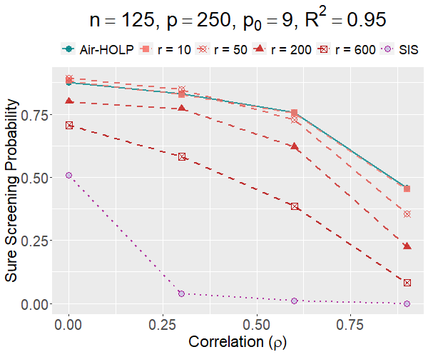
(a)

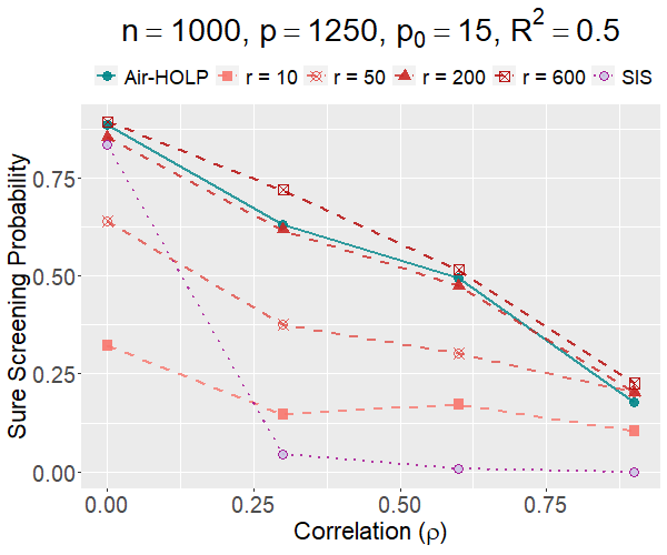
(b)

Figure 1: Line plots comparing the performances of Air-HOLP, Ridge-HOLP and SIS for different levels of correlation in two different simulation settings. For Ridge-HOLP, four values for the penalty parameter are compared: $r=10,50,200,600$.

The SIS by construction works best when features are uncorrelated but can have poor performance when features are highly correlated (Fan and Lv, 2008). In contrast, Ridge-HOLP captures joint relationships between features and the response (Wang and Leng, 2016) and is superior to SIS in highly correlated settings. We confirm this in Figure 1, which also shows the strong performance of Air-HOLP when features are correlated.

In addition, Figure 1 also demonstrates the advantage of adaptive regularization by showcasing two settings were the optimal penalty parameter differ significantly. The lower penalty parameters ($r=10$ and $r=50$) performs well in Figure 1(a) but not as well in Figure 1(b), whereas the higher penalty parameters ($r=200$ and $r=600$) show the opposite trend. Air-HOLP, on the other hand, consistently performs well in both settings.

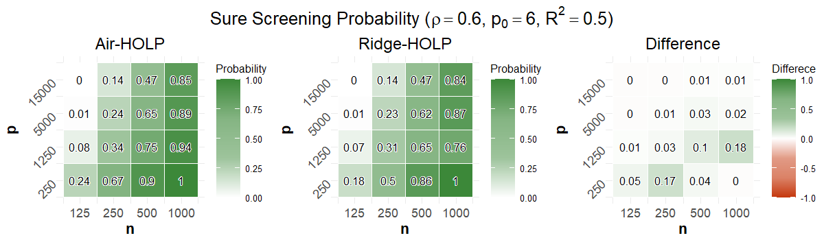
Figure 2: Sure Screening Probability Heatmaps. The left panel shows Air-HOLP, the middle panel shows Ridge-HOLP (with $r=10$), and the right panel shows the difference between Air-HOLP and Ridge-HOLP (Sure Screening Probability of Air-HOLP minus Ridge-HOLP).

We now shift the focus to comparing Air-HOLP and Ridge-HOLP with the recommended penalty parameter of $r=10$, as suggested by Wang and Leng (2016). Across all $1600$ simulation settings, the difference in sure screening probability between Air-HOLP and Ridge-HOLP ranged from $-0.02$ to $0.60$. In $47\%$ of the settings, the sure screening probabilities for Air-HOLP and Ridge-HOLP were equal, typically occurring when both probabilities were either $0$ or $1$. In $45\%$ of the settings, Air-HOLP’s sure screening probability was higher than Ridge-HOLP’s, while in $8\%$ of the settings, it was lower. To better understand the factors influencing this gap in performance, we analyze the impact of $n,p,p_{0}$, and $R^{2}$ on feature screening performance of Air-HOLP and Ridge-HOLP.

Figure 2 showcases the joint effect of the sample size $n$ and the number of features $p$ on the screening performance. The settings $\rho=0.6,p_{0}=6,R^{2}=0.5$ for the presented heat maps in Figure 2 were selected to ensure a diverse range of sure screening probabilities from $0$ to $1$ across the values of $n$ and $p$ for both Air-HOLP and Ridge-HOLP. The selected settings provide a holistic view of the joint impact of $n$ and $p$ on screening performance and comparison. Figure 2 reveals that the performance gap between Air-HOLP and Ridge-HOLP is more pronounced when $n$ is close to $p$ (e.g., when $n=1000$ and $p=1250$). However, the difference can still be significant in other settings (e.g., when $n=500$ and $p=1250$). Moreover, Figure 2 shows that for both Air-HOLP and Ridge-HOLP, a large $n$ has a strong positive impact on screening performance, while a large $p$ has a smaller negative influence. This demonstrates the strong capability of both methods to handle high-dimensional data.

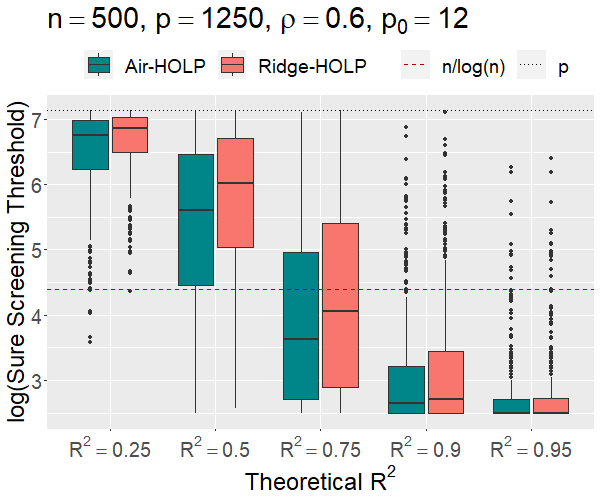
(a) The logarithm of the Sure Screening Threshold vs. Theoretical $R^{2}$.

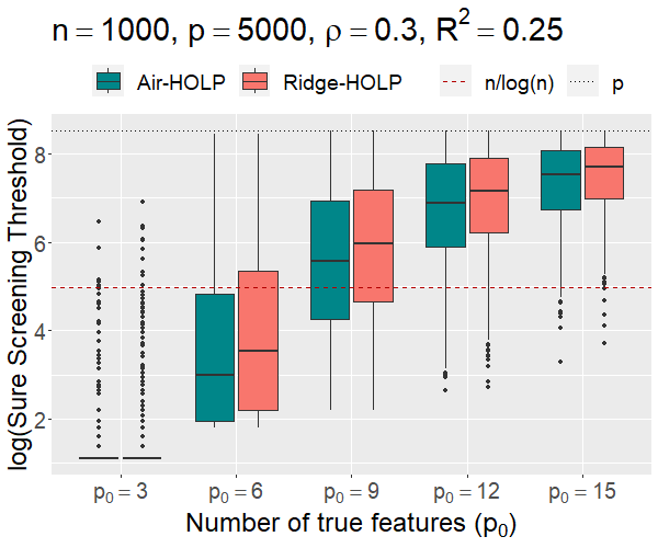
(b) The logarithm of the Sure Screening Threshold vs. the number of true features $p_{0}$.

Figure 3: Boxplots comparing Air-HOLP to Ridge-HOLP (with $r=10$) for different values of $R^{2}$ and $p_{0}$. The red line represents the screening threshold $\lceil n/\log(n)\rceil$. Values below this line indicate simulation runs where all true features are screened in.

Figure 3 showcases the effect of both the number of true features $p_{0}$ and the theoretical $R^{2}$ on the screening performance. The settings $n=500,p=1250,\rho=0.6,p_{0}=12$ for Figure 3(a) and $n=1000,p=5000,\rho=0.3,R^{2}=0.25$ for Figure 3(b) were selected to ensure a diverse range of sure screening thresholds across the values of $p_{0}$ and $R^{2}$ for both Air-HOLP and Ridge-HOLP. These settings provide a comprehensive view of the impact of $p_{0}$ and $R^{2}$ on screening performance. Figure 3(b) illustrates that the performance of both Air-HOLP and Ridge-HOLP declines as the number of true features $p_{0}$ increases. Conversely, Figure 3(a) suggests a direct relationship between the theoretical $R^{2}$, and the screening performance of both methods. Furthermore, Air-HOLP consistently outperforms Ridge-HOLP across most settings of $p_{0}$ and $R^{2}$.

In conclusion, both Air-HOLP and Ridge-HOLP outperform SIS in correlated settings. However, Air-HOLP demonstrates a consistent advantage over Ridge-HOLP across various settings of $n$, $p$, $\rho$, $p_{0}$, and $R^{2}$, achieving higher sure screening probabilities and lower sure screening thresholds as demonstrated in figures 1-3. This showcases the effectiveness of Air-HOLP’s adaptive penalty selection in enhancing feature screening performance.

5 Application to Prostate Cancer Data

We apply Air-HOLP, Ridge-HOLP and SIS to the Tomlins-V2 prostate cancer genetic data of Tomlins et al. (2006) consisting of $n=92$ samples and $p=1288$ genes. The objective of this dataset is to understand the genetic changes that occur as prostate cancer progresses through different stages. The dataset consists of genetic information collected from four stages of prostate cancer.

• Benign Epithelium: Normal, healthy prostate cells.

• Prostatic Intraepithelial Neoplasia: Early changes in cells that might become cancer.

• Prostate Cancer: Actual cancer cells.

• Metastatic Disease: Cancer cells that have spread to other body parts.

Our objective is to compare how well the feature screening methods capture the joint relations between the genes and the responses. We first screen $\lceil n/\log(n)\rceil=21$ genes for each of the four binary responses by each of the three methods. Then, we measure the joint relations between the screened features and the response through the coefficient of multiple correlation, given by

$$\text{Multiple R}=\sqrt{\frac{\|\boldsymbol{\hat{y}}-\boldsymbol{\bar{y}}\|_{2}^{2}}{\|\boldsymbol{y}-\boldsymbol{\bar{y}}\|_{2}^{2}}},$$

where $\boldsymbol{\bar{y}}$ is the mean of $\boldsymbol{y}$ and $\boldsymbol{\hat{y}}$ is the fitted response for a given set of screened features.

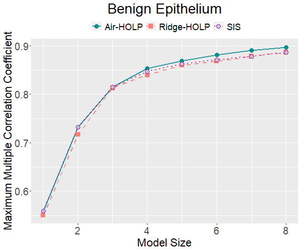
(a)

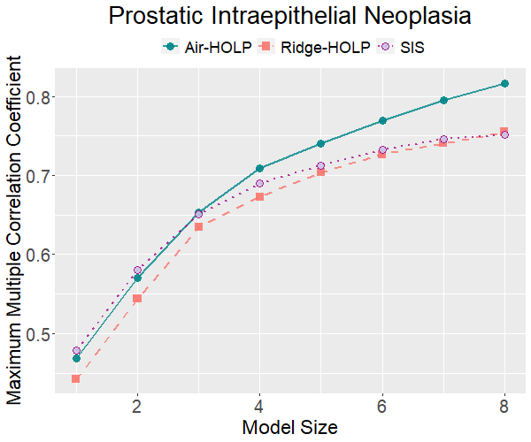
(b)

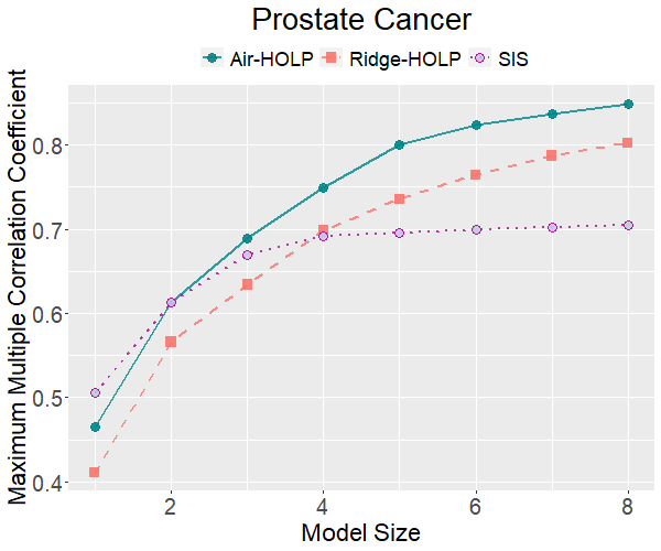
(c)

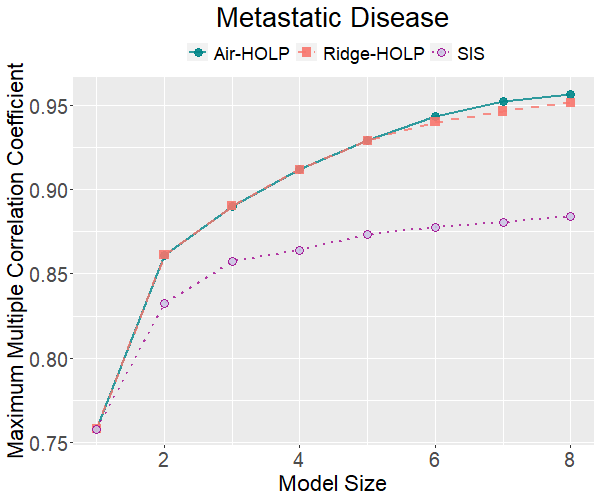
(d)

Figure 4: Maximum Multiple R vs. model size using the screened genes by the competing methods Air-HOLP, Ridge-HOLP, and SIS.

The largest Multiple R for model size $k=1,\ldots,8$ is visualised in Figure 4. This figure shows that Ridge-HOLP and Air-HOLP outperform SIS, because features are correlated in this dataset for all four stages of prostate cancer progression. The maximum Multiple R for Ridge-HOLP and Air-HOLP is higher than that of SIS, especially for larger models. We also observe that for this dataset, Air-HOLP consistently outperforms Ridge-HOLP.

6 Computational Complexity

Air-HOLP shares the same time complexity as Ridge-HOLP. However, Air-HOLP employs an iterative process to update the initial penalty parameter. We investigate how this iterative process impacts the speed of Air-HOLP.

Notably, the eigen decomposition of $\boldsymbol{X}\boldsymbol{X}^{\top}$ in Equation (7) is the only step in Air-HOLP with complexity $O(n^{2}p+n^{3})$, and this step is not repeated. The remaining operations in Air-HOLP have a complexity of $O(np+n^{2})$ or less. To empirically examine the speed and time complexity of Air-HOLP, we compare its execution time to that of Ridge-HOLP and ordinary ridge regression (Ridge-OLS). We generate samples of $\boldsymbol{X}$ and $\boldsymbol{y}$ similarly as in Section 4.1 and use a $12_{th}$ Gen Intel Core i7-1255U ($2$ P-cores, $8$ E-cores, $12$ threads, $1.70$ GHz base frequency, up to $4.70$ GHz turbo frequency). Figure 5(a) confirms that Air-HOLP has the same time complexity as Ridge-HOLP and both methods are considerably faster than Ridge-OLS in high-dimensional settings where $p>>n$. Figure 5(b) shows that Air-HOLP takes roughly twice as long as Ridge-HOLP.

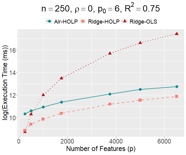
(a) The logarithm of execution time in milliseconds vs. number of features $p$.

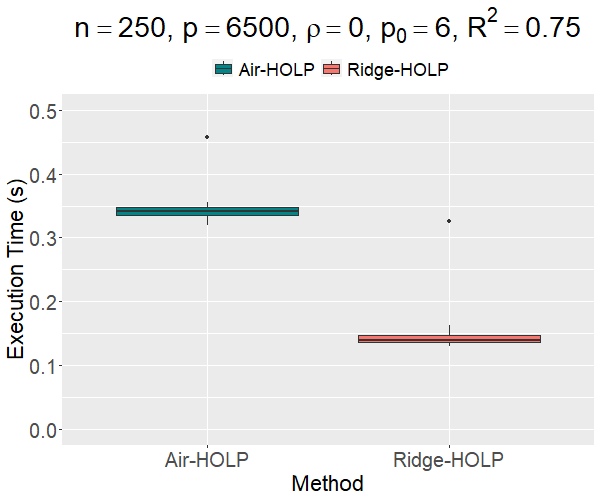
(b) Execution time of Air-HOLP vs. Ridge-HOLP in seconds.

Figure 5: Compression of the execution time between Ridge-OLS, Ridge-HOLP, and Air-HOLP. On the left, we present the trimmed mean of the logarithm of execution time in milliseconds for $10$ simulations ($10\%$ trimming). On the right, we present a boxplot of the execution time in seconds for $10$ simulations.

7 Discussion

Traditional feature screening methods such as SIS measure the marginal relations between features and the response, which can fail when features are correlated. Ridge-HOLP was developed to address this issue and we have now further built on Ridge-HOLP by the development of Air-HOLP, which incorporates adaptively selecting the ridge penalty. This adaptive selection aims to minimize prediction error, thereby effectively balancing the bias-variance trade-off and enhancing feature screening performance.

Through extensive simulation studies, we demonstrated that Air-HOLP consistently outperforms Ridge-HOLP with a fixed penalty parameter across various simulation settings. Air-HOLP achieves higher sure screening probabilities and lower sure screening thresholds. The advantage of Air-HOLP is more pronounced when the number of samples $n$ is closer to the number of features $p$. Additionally, both Air-HOLP and Ridge-HOLP outperformed SIS in correlated settings, making Air-HOLP especially useful for identifying relevant features in high-dimensional correlated data. Moreover, Air-HOLP has the same time complexity as Ridge-HOLP and also enjoys being computationally efficient. We also found that in most simulations, Air-HOLP converged as quickly as in $3$ to $6$ iterations. Therefore, we set the maximum number of iterations to be $10$ in our code.

We further applied Air-HOLP, HOLP and SIS to a prostate cancer genetic dataset. The results confirmed the good performance of Air-HOLP.

References

- Alkhamisi and Shukur (2007) Alkhamisi, M. A. and G. Shukur (2007). A monte carlo study of recent ridge parameters. Communications in Statistics - Simulation and Computation 36(3), 535–547.
- Allen (1971) Allen, D. M. (1971). Mean square error of prediction as a criterion for selecting variables. Technometrics 13(3), 469–475.
- Allen (1974) Allen, D. M. (1974). The relationship between variable selection and data agumentation and a method for prediction. Technometrics 16(1), 125–127.
- Batah et al. (2008) Batah, F. S. M., T. V. Ramanathan, and S. D. Gore (2008). The efficiency of modified jackknife and ridge type regression estimators: A comparison. Surveys in Mathematics and its Applications 3, 111–122.
- Chen et al. (2019) Chen, X., X. Chen, and Y. Liu (2019). A note on quantile feature screening via distance correlation. Statistical Papers 60, 1741–1762.
- Cule and De Iorio (2013) Cule, E. and M. De Iorio (2013). Ridge regression in prediction problems: Automatic choice of the ridge parameter. Genetic Epidemiology 37(7), 704–714.
- Delaney and Chatterjee (1986) Delaney, N. J. and S. Chatterjee (1986). Use of the bootstrap and cross-validation in ridge regression. Journal of Business & Economic Statistics 4(2), 255–262.
- Dorugade and Kashid (2010) Dorugade, A. and D. Kashid (2010). Alternative method for choosing ridge parameter for regression. Applied Mathematical Sciences 4(9), 447–456.
- Fan et al. (2011) Fan, J., Y. Feng, and R. Song (2011). Nonparametric independence screening in sparse ultra-high-dimensional additive models. Journal of the American Statistical Association 106(494), 544–557.
- Fan and Lv (2008) Fan, J. and J. Lv (2008). Sure independence screening for ultrahigh dimensional feature space. Journal of the Royal Statistical Society: Series B (Statistical Methodology) 70(5), 849–911.
- Fan et al. (2014) Fan, J., Y. Ma, and W. Dai (2014). Nonparametric independence screening in sparse ultra-high-dimensional varying coefficient models. Journal of the American Statistical Association 109(507), 1270–1284.
- Fan et al. (2009) Fan, J., R. Samworth, and Y. Wu (2009). Ultrahigh dimensional feature selection: Beyond the linear model. The Journal of Machine Learning Research 10, 2013–2038.
- Golub et al. (1979) Golub, G. H., M. Heath, and G. Wahba (1979). Generalized cross-validation as a method for choosing a good ridge parameter. Technometrics 21(2), 215–223.
- Hall and Miller (2009) Hall, P. and H. Miller (2009). Using generalized correlation to effect variable selection in very high dimensional problems. Journal of Computational and Graphical Statistics 18(3), 533–550.
- Hoerl et al. (1975) Hoerl, A. E., R. W. Kannard, and K. F. Baldwin (1975). Ridge regression: Some simulations. Communications in Statistics - Theory and Methods 4(2), 105–123.
- Hoerl and Kennard (1970) Hoerl, A. E. and R. W. Kennard (1970). Ridge regression: Biased estimation for nonorthogonal problems. Technometrics 12(1), 55–67.
- Hura Ahmad et al. (2006) Hura Ahmad, M. H., R. Adnan, and N. Adnan (2006). A comparative study on some methods for handling multicollinearity problems. MATEMATIKA: Malaysian Journal of Industrial and Applied Mathematics 22, 109–119.
- Kibria (2003) Kibria, B. G. (2003). Performance of some new ridge regression estimators. Communications in Statistics - Simulation and Computation 32(2), 419–435.
- Lawless (1976) Lawless, W. (1976). A simulation study of ridge and other regression estimators. Communications in Statistics - Theory and Methods 5(4), 307–323.
- Li et al. (2012) Li, R., W. Zhong, and L. Zhu (2012). Feature screening via distance correlation learning. Journal of the American Statistical Association 107(499), 1129–1139.
- Liu et al. (2015) Liu, J., W. Zhong, and R. Li (2015). A selective overview of feature screening for ultrahigh-dimensional data. Science China Mathematics 58(10), 1–22.
- Liu et al. (2022) Liu, W., Y. Ke, J. Liu, and R. Li (2022). Model-free feature screening and fdr control with knockoff features. Journal of the American Statistical Association 117(537), 428–443.
- Liu and Li (2020) Liu, W. and R. Li (2020). Variable Selection and Feature Screening, pp. 293–326. Springer.
- Martinez et al. (2011) Martinez, J. G., R. J. Carroll, S. Müller, J. N. Sampson, and N. Chatterjee (2011). Empirical performance of cross-validation with oracle methods in a genomics context. The American Statistician 65(4), 223–228.
- Nomura (1988) Nomura, M. (1988). On the almost unbiased ridge regression estimator. Communications in Statistics - Simulation and Computation 17(3), 729–743.
- Pan et al. (2018) Pan, W., X. Wang, W. Xiao, and H. Zhu (2018). A generic sure independence screening procedure. Journal of the American Statistical Association 114(526), 928–937.
- Qiu and Ahn (2020) Qiu, D. and J. Ahn (2020). Grouped variable screening for ultra-high dimensional data for linear model. Computational Statistics & Data Analysis 144, 106894.
- Samat et al. (2022) Samat, A., E. Li, W. Wang, S. Liu, and X. Liu (2022). Holp-df: Holp based screening ultrahigh dimensional subfeatures in deep forest for remote sensing image classification. IEEE Journal of Selected Topics in Applied Earth Observations and Remote Sensing 15, 8287–8298.
- Tomlins et al. (2006) Tomlins, S. A., R. Mehra, D. R. Rhodes, X. Cao, L. Wang, S. M. Dhanasekaran, S. Kalyana-Sundaram, J. T. Wei, M. A. Rubin, K. J. Pienta, et al. (2006). Integrative molecular concept modeling of prostate cancer progression. Nature Genetics 39(1), 41–51.
- van de Wiel et al. (2021) van de Wiel, M. A., M. M. van Nee, and A. Rauschenberger (2021). Fast cross-validation for multi-penalty high-dimensional ridge regression. Journal of Computational and Graphical Statistics 30(4), 835–847.
- Wang and Leng (2016) Wang, X. and C. Leng (2016). High dimensional ordinary least squares projection for screening variables. Journal of the Royal Statistical Society: Series B (Statistical Methodology) 78(3), 589–611.
- Wang et al. (2021) Wang, X., C. Leng, and T. Boot (2021, 07). Wang and Leng (2016), High-Dimensional Ordinary Least-Squares Projection for Screening Variables, Journal of The Royal Statistical Society Series B, 78, 589–611. Journal of the Royal Statistical Society Series B: Statistical Methodology 83(4), 880–881.
- Wu and Yin (2015) Wu, Y. and G. Yin (2015). Conditional quantile screening in ultrahigh-dimensional heterogeneous data. Biometrika 102(1), 65–76.
- Zhang and Chen (2019) Zhang, J. and X. Chen (2019). Robust sufficient dimension reduction via ball covariance. Computational Statistics & Data Analysis 140, 144–154.
- Zhao et al. (2021) Zhao, B., X. Liu, W. He, and Y. Y. Grace (2021). Dynamic tilted current correlation for high dimensional variable screening. Journal of Multivariate Analysis 182, 104693.
- Zhong et al. (2016) Zhong, W., L. Zhu, R. Li, and H. Cui (2016). Regularized quantile regression and robust feature screening for single index models. Statistica Sinica 26(1), 69.
- Zhu et al. (2011) Zhu, L.-P., L. Li, R. Li, and L.-X. Zhu (2011). Model-free feature screening for ultrahigh dimensional data. Journal of the American Statistical Association 106(496), 1464–1475.