CT scans without X-rays: parallel-beam imaging from nonlinear current flows

Abstract

Parallel-beam X-ray computed tomography (CT) and electrical impedance tomography (EIT) are two imaging modalities which stem from completely different underlying physics, and for decades have been thought to have little in common either practically or mathematically. CT is only mildly ill-posed and uses straight X-rays as measurement energy, which admits simple linear mathematics. However, CT relies on exposing targets to ionizing radiation and requires cumbersome setups with expensive equipment. In contrast, EIT uses harmless electrical currents as measurement energy and can be implemented using simple low-cost portable setups. But EIT is burdened by nonlinearity stemming from the curved paths of electrical currents, as well as extreme ill-posedness which causes characteristic low spatial resolution. In practical EIT reconstruction methods, nonlinearity and ill-posedness have been considered intertwined in a complicated fashion. In this work we demonstrate a surprising connection between CT and EIT which partly unravels the main problems of EIT and leads directly to a proposed imaging modality which we call virtual hybrid parallel-beam tomography (VHPT). We show that hidden deep within EIT data is information which possesses the same linear geometry as parallel-beam CT data. This admits a fundamental restructuring of EIT, separating ill-posedness and nonlinearity into simple modular sub-problems, and yields “virtual radiographs” and CT-like images which reveal previously concealed information. Furthermore, as proof of concept we present VHPT images of real-world objects.

Introduction

One of the marvels of scientific investigation is the occasional discovery of a deep and unexpected connection between seemingly disparate phenomena. In the 19th century, for example, Maxwell surprised the scientific world by connecting electromagnetism and wave theory [26], and Röntgen discovered by chance, while working with cathode rays, how electromagnetic waves in the form of X-rays can be used to view an object’s hidden internal structures [35]. Analogously, we describe here the discovery of an unexpected link between nonlinear electrical imaging and parallel-beam straight-line tomography. This work establishes the existence of physical and mathematical connections between two very different imaging modalities: X-ray computed tomography (CT) and electrical impedance tomography (EIT), and describes the advances these connections bring to the fields of tomographic imaging and inverse problems.

In CT imaging, a technology dating back to the 1970s [21, 5], straight X-ray beams pass through an object and the measured attenuation values are subjected to mathematical inversion, thus forming an image of internal structures. We restrict our discussion of CT to 2D “slice” imaging using parallel-beam geometry, as used by first-generation CT scanners, in which we fix the direction of parallel X-ray beams and record the attenuation of each ray as it travels through the object. After logarithmic transformation a 1D profile function is produced, revealing the total attenuation along each ray. This measurement is repeated for a dense collection of directions, and profile functions from all angles are collected as the columns of a 2D projection array known as a sinogram. Since X-rays travel along straight lines, it is possible to derive a fairly simple linear geometric reconstruction method, as in the widely-used filtered back-projection (FBP) algorithm [30] based upon mathematics formulated by Radon in 1917 [33], to transform the sinogram back to the spatial imaging domain. In the 21st century, iterative methods based on compressed sensing, such as total variation (TV) reconstruction [36], have emerged to provide edge-preserving regularization in situations with limited raw data [39].

EIT on the other hand, which emerged in the 1980s [10], is based on measuring the boundary effects of electrical current flows. We inject harmless electrical currents into a target and measure the voltages arising on electrodes placed on the target’s surface. This boundary data is used to produce an image of the internal electrical conductivity. The difficulties of EIT lie in its nonlinearity and extreme ill-posedness, which until the writing of this present work were considered to be intertwined in a complicated fashion. While X-rays travel in straight lines, this is not so for electrical current, which flows mostly through domains of highest conductivity. Thus in EIT the very structures we are attempting to image will themselves alter the travel paths of the measuring energy, leading to nonlinearity. Linear-ray reconstruction methods therefore cannot be directly applied. Further, while image formation in both CT and EIT is ill-posed in the sense that different targets may produce almost the same measurements, CT is only mildly ill-posed [30] while EIT is extremely ill-posed [2], resulting in reconstructions with characteristically low spatial resolution. Our work demonstrates that EIT data can be nonlinearly processed into a sinogram having exactly the same parallel-beam geometry as data produced by first-generation CT scanners. This is remarkable, as curved electrical current flows differ drastically from the straight paths of X-rays.

Among many EIT reconstruction approaches [28, 14], we focus here on a class of methods based on exponentially-behaving complex geometric optics (CGO) solutions, which permit insight leading to a fundamental restructuring of the EIT problem as well as VHPT imaging. We also restrict ourselves to imaging (approximately) 2D objects, but in practice it is common to produce “slice” images of 3D objects by placing electrodes around the boundary of a cross-sectional plane, thus permitting real-world imaging scenarios.

Our findings lead to both conceptual and practical advances presented in this work. Conceptually, we present an enhanced understanding of the extremely ill-posed nonlinear EIT problem. This involves a modular decomposition where ill-posedness is confined to two linear steps, and all remaining nonlinear steps allow mathematical interpretation. On the practical side, we propose an imaging modality which we call virtual hybrid parallel-beam tomography (VHPT), in which electrical measurements are processed into a sinogram which is produced “virtually,” without actual X-rays. We may then view the columns of the sinogram directly as “virtual radiographs,” or apply standard CT reconstruction techniques to produce a conductivity image.

The Method

We now provide an overview of our method, which invokes deep mathematical connections between EIT and CT, leading directly to practical VHPT imaging.

Figure 1: Method overview. An illustration of our decomposition of the EIT problem into disjoint modules, with a representation of the virtual sinogram at bottom right. Arrow type and color indicate the type of operation; red: ill-posed, black: well-posed, straight: linear, and curved: nonlinear. We flow through (A)-(G): (A) process EIT measurements into a DN map, (B) solve a boundary integral equation to yield CGO traces, (C^′)-(C^′′′) apply a windowed Fourier transform and two simple linear operations, (D) remove higher-order scattering terms through machine learning, (E) apply 1D deconvolution separately to each column, (F) apply FBP, TV, or other CT reconstruction algorithm, (G) apply a simple algebraic formula. In this work, (D) is achieved through generalization of (E). Ill-posedness is completely confined to linear steps (E) and (F), with (E) containing almost all of it. Process flows for D-bar and cost-function-based methods are included for comparison.

Mathematical Model

Let $\Omega\subset\mathbb{R}^{2}$ be the unit disc and let the electrical conductivity $\sigma:\Omega\rightarrow\mathbb{R}$ satisfy $0<c^{-1}\leq\sigma(x)\leq c,\;x\in\Omega.$ We begin by considering infinite-precision EIT measurements of the unknown conductivity $\sigma$ as described in [12]. In this ideal model called the inverse conductivity problem, one applies a voltage distribution along the boundary $\partial\Omega$ and measures the current density through the boundary. Letting $u$ denote the electric potential, the propagation of the electric field through $\Omega$, along with a known boundary voltage distribution, is modeled by the elliptic PDE $\nabla\cdot\sigma\nabla u=0$ in $\Omega,$ with Dirichlet condition $u|_{\partial\Omega}$ specified. We seek to recover $\sigma$ satisfying this boundary value problem, given knowledge of the boundary voltage-to-current map, also called the Dirichlet-to-Neumann (DN) map $\Lambda_{\sigma}:H^{1/2}(\partial\Omega)\to H^{-1/2}(\partial\Omega)$, given by $\Lambda_{\sigma}:u|_{\partial\Omega}\longmapsto\sigma\frac{\partial u}{\partial\nu}\;\mbox{on }{\partial\Omega},$ where $\nu$ is the outward unit normal vector to $\partial\Omega$.

VHPT Imaging, Step-by-Step

Here we describe the mathematical and computational steps of VHPT imaging, following the diagram given in Figure 1.

Step (A): EIT Data to DN Map

As a first step, we present an algorithm which transforms real-world data measurements into a mathematically ideal discrete DN map $\boldsymbol{\Lambda}_{\sigma}$. This method may be viewed as a practical implementation of theory developed in [17]. We assume two DN matrices computed from real-world EIT measurements: the “target” matrix $\boldsymbol{\Lambda}_{\mathrm{trg}}$ representing measurements collected at the boundary of the target object, and the “calibration” matrix $\boldsymbol{\Lambda}_{\mathrm{clb}}$ collected on a reference domain (e.g. a homogeneous tank). We further assume two simulated DN matrices corresponding to a homogeneous domain where $\sigma=1$: $\boldsymbol{\Lambda}_{1}$, computed under the mathematically ideal continuum model [13]; and $\boldsymbol{\Lambda}_{1}^{\mathrm{cem}}$, simulated using the “complete electrode model” [13] which takes into account various physical effects of electrodes, by solving the forward EIT problem using finite element methods. The final DN map is obtained via $\boldsymbol{\Lambda}_{\sigma}=(\widetilde{\boldsymbol{\Lambda}}_{\sigma}^{-1}+(\widetilde{\boldsymbol{\Lambda}}_{\sigma}^{T})^{-1})/2$, where $\widetilde{\boldsymbol{\Lambda}}_{\sigma}=(\boldsymbol{\Lambda}_{1}^{\mathrm{cem}})^{-1}\boldsymbol{\Lambda}_{\mathrm{clb}}(\boldsymbol{\Lambda}_{\mathrm{trg}})^{-1}-(\boldsymbol{\Lambda}_{1}^{\mathrm{cem}})^{-1}+(\boldsymbol{\Lambda}_{1})^{-1}.$ This is a form of difference imaging, as opposed to the absolute imaging scenario in which $\boldsymbol{\Lambda}_{\sigma}$ would be computed using only one set of experimentally collected measurements, $\boldsymbol{\Lambda}_{\mathrm{trg}}$. Difference imaging in EIT is well-known to provide significant advantages over absolute imaging in terms of robustness to noise and modeling errors [8]. Details of this calibration approach are provided in the SI Appendix.

Step (B): DN Map to CGO Traces

Next, we follow [7, 6] to solve for the traces of certain complex geometric optics (CGO) functions $\omega^{\pm}=\omega^{\pm}(x,k)$ related to the conductivity $\sigma=\sigma(x)$, where $x$ is the spatial domain variable and $k$ is an introduced complex spectral parameter. Consider solutions $f_{\pm\mu}(x,k)=e^{ikx}(1+\omega^{\pm}(x,k))$ of the Beltrami-type equation $\bar{\partial}f_{\mu}=\mu\overline{\partial f_{\mu}},$ where the Beltrami coefficient $\mu$ is given by $\mu:=\frac{1-\sigma}{1+\sigma},$ and $\partial=\frac{1}{2}(\frac{\partial}{\partial x_{1}}-i\frac{\partial}{\partial x_{2}})$ and $\overline{\partial}=\frac{1}{2}(\frac{\partial}{\partial x_{1}}+i\frac{\partial}{\partial x_{2}})$ are the complex Wirtinger derivatives. In [7] it is shown that $\omega^{\pm}|_{\partial\Omega}$ may be obtained from knowledge of $\Lambda_{\sigma}$ by solving the boundary integral equation

$${M_{\pm\mu}(\,\cdot\,,k)|_{\partial\Omega}+1=({\mathcal{P}}_{\pm\mu}^{k}+{\mathcal{P}}_{0})M_{\pm\mu}(\,\cdot\,,k)|_{\partial\Omega},}$$ (1)

where $M_{\pm\mu}(x,k):=1+\omega^{\pm}(x,k)$ and ${\mathcal{P}}_{\pm\mu}^{k}$ and ${\mathcal{P}}_{0}$ are certain projection operators computed directly from the DN map $\Lambda_{\sigma}$ (see the SI Appendix). It is further shown in [18] that the CGO solutions $\omega^{\pm}$ can be written as a scattering series $\omega^{\pm}=\sum_{j=1}^{\infty}\omega_{j}^{\pm}.$ While the leading order term $\omega_{1}^{+}$ contains relevant information of the singularities of $\mu$ and thus of the conductivity $\sigma$, in the inverse problem setting with unknown conductivity we can only compute the full series $\omega^{\pm}$ and there is no formula to solve for $\omega_{1}^{+}$. However, in [18] it is also shown that by subtracting $\omega^{-}$ from $\omega^{+}$, one eliminates all even terms $\omega_{2j}^{+}$ in the scattering series of $\omega^{+}$. We therefore denote $\omega_{\text{odd}}^{+}:=\omega^{+}-\omega^{-}$. Since in what follows we will focus on the “plus” cases $\omega_{1}^{+}$ and $\omega_{\text{odd}}^{+}$, for notational simplicity we denote these functions by $\omega_{1}$ and $\omega_{\text{odd}}$, respectively. After solving (1) twice to obtain $\omega_{\text{odd}}$ from the solutions $M_{\pm\mu}$, we integrate the functions $\omega_{\text{odd}}$ to get a scattering operator $\widetilde{T}_{\text{odd}}\mu(\tau,\varphi)$ with parameters $\tau\in{\mathbb{R}}$ and $\varphi\in[0,2\pi]$ (depicted in Figure 1):

$$\widetilde{T}_{\text{odd}}\mu(\tau,\varphi):=\frac{1}{2\pi i}\int_{\partial\Omega}\omega_{\text{odd}}(x,\tau e^{i\varphi})\mathop{}\!\mathrm{d}x.$$

Steps (C^′)–(C^′′′): CGO Traces to CGO Sinogram

Noise in the data $\boldsymbol{\Lambda}_{\sigma}$ causes inaccuracy in the solution of the boundary integral equation (1) which grows with $|\tau|$. As a low-pass filter, we apply a one-dimensional windowed Fourier transform to the scattering operator $\widetilde{T}_{\text{odd}}\mu(\tau,\varphi)$. We therefore restrict integration to an interval $[-R,R]$ and insert a Gaussian function $e^{-a\tau^{2}}$ with suitable parameter $a>0$ into the Fourier integral:

$$T_{\text{odd}}\mu(t,\varphi)=\frac{1}{2\pi i}\int_{-R}^{R}e^{-a\tau^{2}}e^{-it\tau}(\widetilde{T}_{\text{odd}}\mu(\tau,\varphi))\mathop{}\!\mathrm{d}\tau,$$ (2)

where the variable $t\in\mathbb{R}$ is called the pseudo-time. By this Fourier windowing, the noisy parts of the signal will be set to zero, but as a trade-off, the resulting complex-valued $T_{\text{odd}}\mu(t,\varphi)$ has blurring in the pseudo-time domain. In practical computations, this corresponds to blurring along the columns of the matrix approximation to $T_{\text{odd}}\mu(t,\varphi)$, as depicted in Figure 1. To compute the real-valued “projection data” function from the complex-valued version, we multiply with a complex phase factor and then integrate to get the CGO sinogram $R_{\text{odd}}\mu(s,\varphi)=\int_{-\infty}^{s}\frac{e^{-i\varphi}}{2\pi i}T_{\text{odd}}\mu(t,\varphi)\mathop{}\!\mathrm{d}t.$

Steps (D)–(E): CGO Sinogram to Sharp Sinogram

The CGO sinogram is blurred due to the necessary Fourier windowing process. Moreover, due to our unavoidable use of $\omega_{\text{odd}}$ in place of the ideal $\omega_{1}$, the quantity $R_{\text{odd}}\mu(s,\varphi)$ does not exactly match the desired theoretical framework. Based on [18], the ideal quantity $\omega_{1}$ would correspond to the Fourier integral $T_{1}\mu$ and projection data $R_{1}\mu$, as opposed to $R_{\text{odd}}\mu$. This discrepancy may be rectified by using a convolutional neural network (CNN) to remove the higher order terms of the scattering series in the projection domain, which corresponds to step (D) in Figure 1. One could follow this machine-learning process with any linear deconvolution algorithm (step (E)) to correct the blur. In our implementation, however, we found it was efficient to perform steps (D) and (E) simultaneously by training a single neural network to perform the deconvolution operation $\text{NN}_{\theta}(R_{1}\mu)\approx R\mu,$ where $\theta$ is the learned parameter vector. The training inputs are ideal CGO sinograms computed from numerically simulated functions $\omega_{1}$, given by $R_{1}\mu(s,\varphi)=\int_{-\infty}^{s}\frac{-e^{i\varphi}}{2\pi i}(g*T_{1})\mu(t,\varphi)\mathop{}\!\mathrm{d}t,$ where $g=g(t)$ is the inverse Fourier transform of $e^{-a\tau^{2}}$ and $T_{1}\mu(t,\varphi)$ is computed from $\omega_{1}$ and is analogous to (2). The ground truth $R\mu$ is the Radon transform of $\mu$, defined as $R\mu(s,\varphi)=\int_{x\cdot\varphi=s}\mu(x)dx.$ After training, the network generalizes and can be used instead with inputs given by the CGO sinograms $R_{\text{odd}}\mu$ computed from the EIT data. The network outputs sharp VHPT sinograms $S\approx R\mu$, where the higher-order scattering terms have consequently been removed. Details regarding network architecture and training are provided in the SI Appendix.

Steps (F)–(G): Sharp Sinogram to Reconstruction

Remarkably, the sharpened sinogram embodies exactly the same geometry as one expects from parallel-beam X-ray tomography, but is produced without ionizing radiation. Geometric information about the target’s interior may be extracted directly by viewing columns of the sinogram, but if desired we can transform this projection data into the spatial image domain using standard (mildly ill-posed) CT reconstruction methods. This linear inversion process (F) along with the previous linear deconvolution problem (E) together contain all ill-posedness of the VHPT chain, admitting an enhanced understanding of EIT within the framework of nonlinear ill-posed inverse problems. Application of FBP, TV, or another standard CT reconstruction method to the sinogram will yield the Beltrami coefficient $\mu$. For this work we applied TV reconstruction, as described in greater detail in the SI appendix. The conductivity $\sigma$ satisfies $\sigma=(1-\mu)/(1+\mu)$, and we apply this formula in step (G) to yield a conductivity image, thus completing the VHPT process.

Results

Conceptual Discoveries

Aside from providing a practical imaging technique, the previously described VHPT method yields a conceptual discovery which brings enhanced clarity to the EIT problem. The article [18] revealed a linear FBP framework hidden inside the nonlinear inverse problem of EIT, a breakthrough which was based on deep mathematical analysis [15, 19]. We now extend these results by presenting a fundamental restructuring of the decades-old EIT problem, as illustrated in Figure 1. Here we see the remarkable fact that the very complicated EIT problem may be modularly decomposed into a series of well-posed nonlinear problems (black arrows in Figure 1), followed by two ill-posed but linear inverse problems (red arrows). One of these ill-posed modules is the standard (mildly ill-posed) CT reconstruction problem (solvable via FBP or TV, for example), and the other is simply a compilation of classical linear one-dimensional Gaussian deconvolution problems. In addition, all but one of the well-posed nonlinear problems are mathematically explicit. The sole non-explicit step in the process (step (D) in Figure 1) can be viewed as stripping an infinite non-physical scattering series of its higher-order terms. In this work, we show that (D) and (E) may in fact be completed simultaneously using machine learning, although one can approach them as separate problems. The severely ill-posed and nonlinear processes labeled “cost-function-based methods” and “D-bar” in Figure 1 are not part of the VHPT imaging chain, but provide comparison with other common EIT reconstruction algorithms wherein ill-posedness and nonlinearity are intertwined.

Practical Reconstructions

In Figure 2 we present VHPT conductivity reconstructions (C) of real-world objects, produced by applying total variation reconstruction [9] to virtual parallel-beam sinograms (B) computed from EIT measurements. Target datasets I-III, consisting of voltage measurements taken on all electrodes for each current injection, were collected using the ACT5 EIT system at Colorado State University [38]. Current injection at peak amplitude 0.35 mA was applied on 32 electrodes according to a trigonometric basis. We constructed each target to consist of a circular tank filled with saline solution of conductivity 2.7 mS/cm, with various homogeneous agar inclusions having conductivity either 0.5 mS/cm (yellow agar) or 3.7 mS/cm (red agar). The resulting VHPT reconstructions (C) in Figure 2 depict conductivity contrasts of the target interior, ranging from lowest (black) to highest (white) conductivity as compared to background.

In Figure 3 we provide a sampling of virtual radiographs (columns of the sinogram) corresponding to virtual measurement angles (A),(B),(C). Resistive yellow inclusions correspond to peaks in the radiographs, while conductive red inclusions result in valleys. Observe that the open mouth of the Pac-Man in target III corresponds to a sharp “notch” in the radiograph, most visible for angle (B), although this sharp feature is smoothed out in the regularized TV reconstruction. This simple example provides a glimpse of the practical advantages possible with this decomposition of the EIT problem: by removing some ill-posedness from the inversion process, virtual radiographs can reveal important geometric information that may be lost during the full reconstruction process.

I

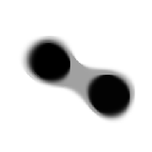
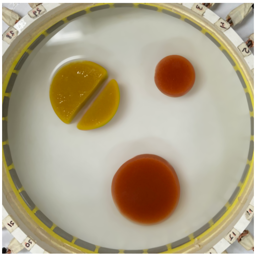
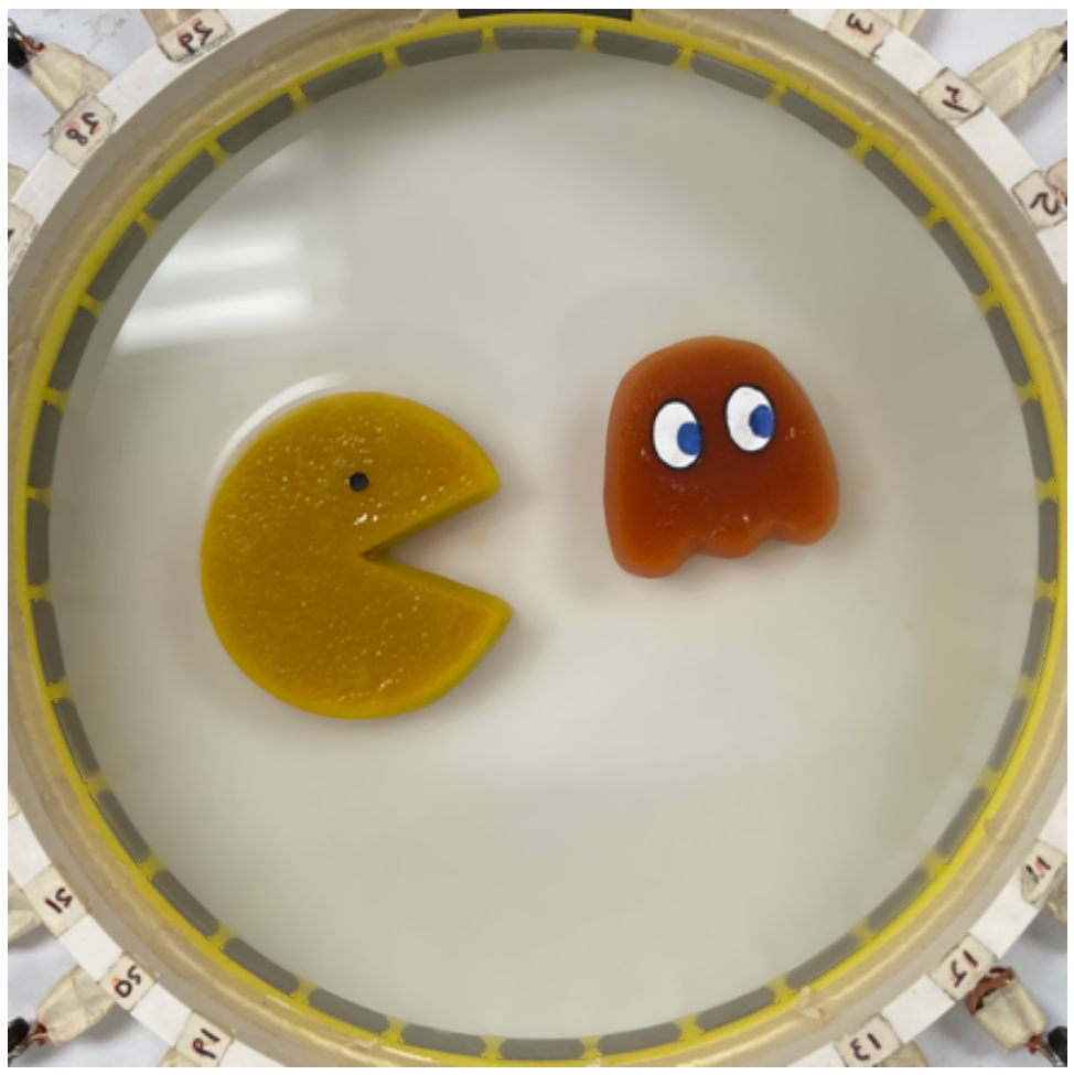
A

B

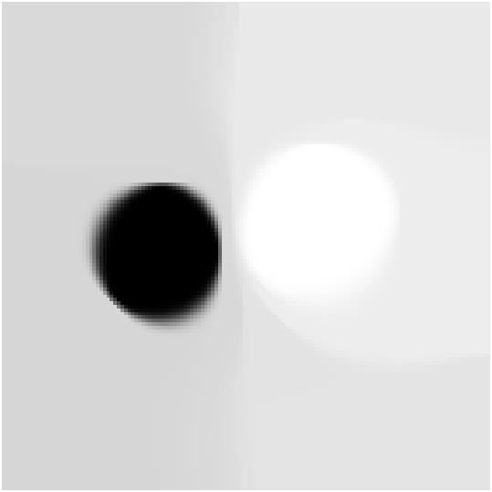
C

Figure 2: Results. (A): The experimental setup for collection of the EIT target datasets I, II, III with 32 electrodes. Yellow agar inclusions are resistive and red inclusions are conductive, as compared to background. (B): VHPT virtual (deblurred) sinogram for targets I, II, III. (C): VHPT conductivity reconstructions via total variation regularization for targets I, II, III.

II

III

I

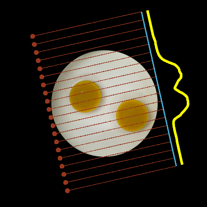
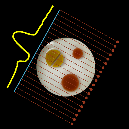
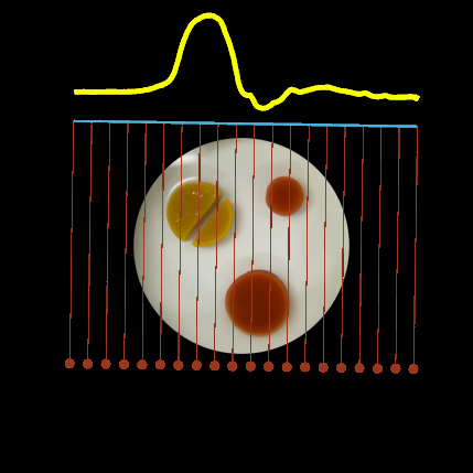
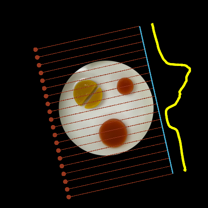
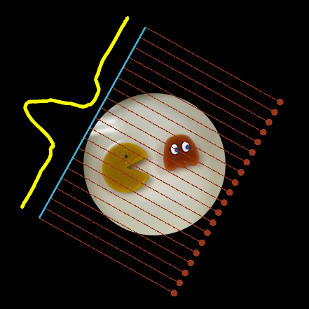
A

B

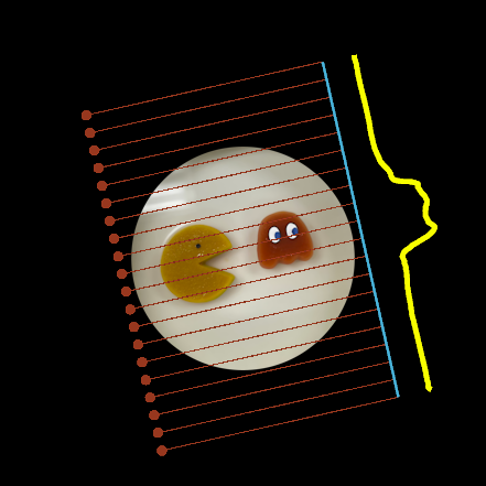
C

Figure 3: Sinogram profiles, superimposed on cropped photos from data collection, with illustrations of virtual X-ray beams. A sampling of virtual radiographs for targets I, II, III from various directions (A), (B), (C) are plotted in yellow. These are the individual columns of the VHPT sinogram, representing the attenuation of virtual parallel X-ray beams (in red). On III(B) a red arrow indicates a sharp “notch” in the radiograph corresponding to the open mouth of the Pac-Man.

II

III

Discussion

For five decades now, CT has been a standard technique for uncovering the internal structure of objects, due to its straightforward linear geometry and relatively mild ill-posedness. The EIT problem is much more challenging than that of CT, and these difficulties lead to characteristic blur in EIT images. However, EIT has advantages in its portability, low cost, and use of nonionizing measurement energy; and EIT has shown promise for example in the evaluation of lung function in cystic fibrosis patients [27], treatment and monitoring of COVID-19 patients [23, 31, 44], classification of stroke [1], and monitoring fluid flows in chemical and process engineering [32, 42].

Nachman’s 1996 study [29] paved the way for the now well-established CGO-based D-bar reconstruction method for EIT [40, 22, 28], wherein the characteristic blurriness of EIT images has been traced back to a nonlinear Fourier-domain viewpoint [25]. The exponential behavior of CGO solutions is used to define a nonlinear Fourier transform for 2D EIT, which is subjected to low-pass filtering at a cutoff frequency dependent on the signal-to-noise ratio, offering regularization but causing blur. Strategies for improving D-bar reconstructions have included the removal of nonlinear blur in a post-processing step [20], introduction of a Schur-complement based prior [37], and the inclusion of spatial priors into the nonlinear Fourier domain [3]. However, in all of these approaches, ill-posedness and nonlinearity were considered to be fundamentally linked.

In this work we invoke related ideas of custom Fourier analysis to solve the EIT problem and yield high-quality reconstructions, but we do so in a way which decouples nonlinearity and ill-posedness. One of the main benefits of the proposed approach, therefore, is enhanced interpretability. The complicated EIT problem is decomposed into a series of comparatively simple modules which isolate the most troublesome features. Ill-posedness is contained entirely within two well-understood modules, permitting application of standard linear techniques. Only the well-posed nonlinear step (D) in Figure 1 truly necessitates black-box machine learning, and this module permits clear geometric interpretation. All other nonlinear steps may be treated using explicit analytic methods. Furthermore, we anticipate scholars and engineers will find independent uses for intermediate outcomes within the imaging chain (e.g. as inputs to machine learning algorithms), as has already been demonstrated in [1].

New Directions

On top of conceptual clarity, our decomposition of the EIT problem unlocks numerous future imaging possibilities. Via the (deblurred) parallel-beam sinogram, the plethora of reconstruction methods published for linear X-ray tomography in the preceding decades becomes suddenly relevant for nonlinear EIT. Furthermore, while a conductivity image may be readily computed from the sinogram if needed, important geometric information is present in individual columns of the sinogram. These can be interpreted directly if desired, thus removing some ill-posedness from the imaging process. These “virtual radiographs” can for example reveal certain sharp features that may be lost in the regularized conductivity reconstruction, as we have demonstrated in this work.

In industrial process control for instance, one could generate virtual radiographs to monitor multiphase flow in pipes without X-ray radiation, which in current set-ups necessitates highly specialized facilities, expensive equipment, and radiation protection[32]. The proposed method could greatly reduce the complexity and size of tomographic measuring devices and eliminate risks associated with ionizing radiation. As one example, consider the problem of monitoring the flow of a mixture of opaque fluid and other substances inside a pipeline, e.g. in petroleum platforms where long risers transport a mixture of gas, petroleum, and water from the ocean floor. An inexpensive belt of electrodes attached around the pipeline would enable EIT measurements. By approximating the measurement domain as a 2D cross-section of the target, we may compute the VHPT sinogram repeatedly at an appropriate frame rate and plot the time traces of one or more fixed columns as rows in a video frame. Such rolling “virtual fluoroscopy” would offer an “X-ray” view of inhomogeneities traveling past the 2D measurement domain, without any actual X-rays.

We further anticipate the conceptual and practical advances developed here will extend analogously to other ill-posed problems, including diffuse optical tomography and electrical capacitance tomography. Such modalities have much in common with EIT, including the use of nonlinear wave phenomena as measurement energy and the recovery of an unknown PDE coefficient as image reconstruction. These possibilities, so far unexplored, may present new directions for advancement in many fields. CGO solutions have been fruitful in inverse problems related to the Helmholtz and heat equations, and we anticipate VHPT-type methods to be possible for those as well.

Data Availability and Reproducibility

All data and code necessary to reproduce the VHPT reconstructions provided in this work are available in [4].

Supplementary materials

In this Appendix we elaborate upon some technical and mathematical details behind the VHPT techniques described in the main text of our work. This material is considered optional reading for those readers who desire deeper understanding of VHPT.

Details of Computing the DN Matrix

Here, we provide details of our calibration approach for completing step (A) of the VHPT imaging chain described in the main text. This involves computing a DN matrix $\boldsymbol{\Lambda}_{\sigma}$ from real-world EIT measurements, and our approach may be thought of as a practical implementation of the ideas presented in [17]. To compute a numerical solution of the boundary integral equation

$${M_{\pm\mu}(\,\cdot\,,k)|_{\partial\Omega}+1=({\mathcal{P}}_{\pm\mu}^{k}+{\mathcal{P}}_{0})M_{\pm\mu}(\,\cdot\,,k)|_{\partial\Omega},}$$ (3)

described in the main text, we must first compute a matrix approximation $\boldsymbol{\Lambda}_{\sigma}$ of the DN map $\Lambda_{\sigma}$ associated with the continuum model

$$\nabla\cdot\sigma\nabla u =0\quad\mbox{ in }\Omega,$$ (4)

$$u =f\quad\mbox{ on }\partial\Omega.$$ (5)

In practical real-world computations, using $L$ electrodes arranged around $\partial\Omega$, we measure the voltage distribution arising from each of $L-1$ linearly independent trigonometric current patterns, applied with peak amplitude $I_{0}$. Raw current measurements are rearranged into a matrix $J$ of size $L\times(L-1)$, where the $n$th column corresponds to the basis functions

$$\phi_{n}(\theta_{\ell})=\begin{cases}\displaystyle I_{0}\cos\left(\frac{(n+1)}{2}\theta_{\ell}\right)&\quad\mbox{odd }n,\\[11.62495pt] \displaystyle I_{0}\sin\left(\frac{n}{2}\theta_{\ell}\right)&\quad\mbox{even }n,\end{cases}$$ (6)

$n=1,\dots,L-1$, where $\theta_{\ell},\;\ell=1,\dots,L$ are taken to be electrode centers.

Corresponding voltage matrices $V_{\mathrm{clb}}$ and $V_{\mathrm{trg}}$ are formed for the calibration data (e.g. a homogeneous domain) and the target data, respectively. From these current and voltage measurements we form a discrete matrix approximation $\boldsymbol{\Lambda}_{\sigma}$ to the DN map $\Lambda_{\sigma}$ via a novel calibration approach which we describe in detail later in this section.

If instead of considering the Dirichlet boundary condition (5) to the equation (4) we consider the Neumann boundary condition

$$\sigma\frac{\partial u}{\partial\nu}=\phi\quad\text{on }\partial\Omega$$

satisfying $\int_{\partial\Omega}u\,ds=0$, then the Neumann-to-Dirichlet (ND) map ${\cal R}_{\sigma}:H^{-1/2}_{\diamond}(\partial\Omega)\to H^{1/2}_{\diamond}(\partial\Omega)$ is given by

$${\cal R}_{\sigma}:\phi\longmapsto u_{|_{\partial\Omega}}.$$ (7)

Here $H^{s}_{\diamond}(\partial\Omega)$ spaces consist of functions in the standard Sobolev space $H^{s}(\partial\Omega)$ having mean value zero. Given a set of basis functions $\{\phi_{n}\}_{n>0}$ on $\partial\Omega$, an infinite discrete matrix approximation $\mathbf{R}_{\sigma}$ to the ND map (7) can be constructed by first computing $\mathcal{R}_{\sigma}\phi_{n}$, $n>0$ and then evaluating the inner products

$$\langle\phi_{m},\mathcal{R}_{\sigma}\phi_{n}\rangle=:(\mathbf{R}_{\sigma})_{mn},$$

where $\langle\cdot,\cdot\rangle$ denotes the usual inner product in $L^{2}(\partial\Omega)$. Inverting this matrix $\mathbf{R}_{\sigma}$, one has a matrix approximation $\boldsymbol{\Lambda}_{\sigma}$ of the DN map $\Lambda_{\sigma}$ restricted to the subspace of zero-mean functions.

However, in practical applications instead of continuum data one has a finite number of voltage and current measurements. The most accurate and widely used mathematical model for the electrode measurements is the complete electrode model (CEM) [41]. Let $e_{\ell}\subset\partial\Omega$, $\ell=1,\dots,L$ be disjoint open paths modeling the electrodes. The CEM is defined by the conductivity equation (4) and the following boundary conditions:

$$z_{\ell}\,\sigma\frac{\partial u}{\partial\nu}+u =V_{\ell},\quad\,\text{on }e_{\ell},\;\ell=1,\ldots,L$$ (8)

$$\frac{\partial u}{\partial\nu} =0,\quad\;\text{ on }\partial\Omega\setminus\cup_{\ell=1}^{L}e_{\ell}$$ (9)

$$\int_{e_{\ell}}\sigma\frac{\partial u}{\partial\nu}\mathop{}\!\mathrm{d}s =I_{\ell},\quad\,\,\ell=1,\dots,L,$$ (10)

where $V_{\ell}$ is the constant electric potential on electrode $e_{\ell}$, $z_{\ell}$ is the contact impedance at electrode $e_{\ell}$, and $I_{\ell}$ denotes the net current on electrode $e_{\ell}$. The absolute measurements of the CEM are modeled by the electrode current-to-voltage map ${\cal R}_{\sigma}^{\text{cem}}:{\mathbb{R}}^{L}_{\diamond}\to{\mathbb{R}}^{L}_{\diamond}$ given by

$${\cal R}_{\sigma}^{\text{cem}}:I\longmapsto V.$$

Analogously to the formation of the infinite discrete $\mathbf{R}_{\sigma}$ computed from the continuum model, we can calculate a finite matrix approximation $\mathbf{R}^{\text{cem}}_{\sigma}$ of the electrode current-to-voltage map ${\cal R}_{\sigma}^{\text{cem}}$ and then invert this matrix to compute a matrix approximation $\boldsymbol{\Lambda}^{\text{cem}}_{\sigma}$ of the DN map $\Lambda_{\sigma}$. However, in this study we follow ideas presented in [17] and use CEM data to form an approximation $\mathbf{Y}^{\text{cem}}_{\sigma}$ to the relative continuum ND map

$$\Upsilon_{\sigma}:={\cal R}_{\sigma}-{\cal R}_{1},$$

where ${\cal R}_{1}$ is the ND map corresponding to homogeneous conductivity $\sigma\equiv 1$ on $\Omega$. Then, from $\mathbf{Y}^{\text{cem}}_{\sigma}$ we compute the desired finite DN matrix $\boldsymbol{\Lambda}_{\sigma}$.

Since we take $\Omega$ to be the unit disc, we assume the center of electrode $e_{\ell}$ is given by $x_{\ell}=\text{e}^{i\theta_{\ell}}$ where ${\theta_{\ell}=\ell\frac{2\pi}{L}}$, for $\ell=1,\ldots,L$. In this study, the continuum current patterns are given by the trigonometric basis functions (6). Under the previous assumptions the numerical algorithm of the method proposed in [17] to compute a matrix approximation of the continuum DN map $\Lambda_{\sigma}$ reduces to the following steps:

• Step 1: For even $L$, take $n=1,\ldots,L-2$ and define

  $$I^{(n)}:=\frac{2\pi}{L}\left[\phi_{n}(\theta_{1}),\ldots,\phi_{n}(\theta_{L})\right]^{T}\in\mathbb{R}^{L}_{\diamond}.$$

  We discard $I^{(L-1)}$ since the CGO-based reconstruction method described in the main text requires an even number of basis functions to ensure invertibility of the matrix approximation to a tangential derivative operator used in the construction of the projection operators $\mathcal{P}^{k}_{\pm\mu}$ and $\mathcal{P}_{0}$ in equation (3) (see (11), defined later in this Appendix). If $L$ is even (as is the case with most EIT systems), then $L-1$ is odd and we must therefore eliminate this extraneous current pattern.

• Step 2: For $n=1,\ldots,L-2$, perform the measurements of CEM with $I^{(n)}$ as input current to retrieve

  $$V_{\sigma}^{(n)} ={\cal R}_{\sigma}^{\text{cem}}I^{(n)}\in{\mathbb{R}}^{L}_{\diamond}$$

  $$V_{1}^{(n)} ={\cal R}_{1}^{\text{cem}}I^{(n)}\in{\mathbb{R}}^{L}_{\diamond}.$$

  Then, define $U_{\sigma}^{(n)}=V_{\sigma}^{(n)}-V_{1}^{(n)}$ and form the matrix $\mathbf{U}=[U^{(1)}\,U^{(2)}\ldots U^{(L-2)}].$

• Step 3: Construct the matrix $\mathbf{I}=[I^{(1)}\,I^{(2)}\ldots I^{(L-2)}].$

• Step 4: Compute a matrix approximation of the relative electrode current-to-voltage map as

  $$\mathbf{Y}^{\text{cem}}_{\sigma}=\mathbf{I}^{T}\mathbf{U}.$$

• Step 5: Finally, a matrix approximation of the DN map $\Lambda_{\sigma}$ acting on the the basis (6) is given by

  $$\boldsymbol{\Lambda}^{\text{cem}}_{\sigma}=(\mathbf{Y}^{\text{cem}}_{\sigma}+\mathbf{R}_{1})^{-1},$$

  where $\mathbf{R}_{1}$ is an ideal reference ND matrix given by

  $$\mathbf{R}_{1}=\text{diag}(1,1,\frac{1}{2},\frac{1}{2},\ldots,\frac{2}{L-2},\frac{2}{L-2}).$$

This process may be thought of as a form of difference imaging, in that to compute the approximate DN map $\boldsymbol{\Lambda}^{\text{cem}}_{\sigma}$ we use the difference measurements $\mathbf{U}=\mathbf{V}_{\sigma}-\mathbf{V}_{1}$, as opposed to the absolute imaging scenario wherein we would compute and invert the finite matrix approximation $\mathbf{R}^{\text{cem}}_{\sigma}$ of the current-to-voltage map ${\cal R}_{\sigma}^{\text{cem}}$. In practical computations with experimental data, EIT difference imaging has been demonstrated to provide significant advantages over absolute imaging in terms of robustness to modeling errors and measurement noise [8].

To compute the voltage matrix $\mathbf{U}$ in Step 2 one needs a matrix approximation of ${\cal R}_{1}^{\text{cem}}$. Therefore, to directly implement the method proposed in [17] using real-world data, one needs EIT measurements corresponding to homogeneous unit conductivity, that is $\sigma=1$, but this is not always possible. However, in laboratory experiments we may collect measurements on an “empty” tank filled with homogeneous saline. Here, we present a novel calibration step that allows us to approximate ${\cal R}_{1}$ from such empty-tank measurements. Then, applying the same calibration step to the measurements collected on the target, we obtain an approximation of ${\cal R}_{\sigma}$, which subsequently yields a good matrix approximation of $\Lambda_{\sigma}$ in the spirit of the method proposed in [17]. The procedure consists of the following steps:

• Step (i): Collect EIT measurements on a tank filled with homogeneous saline solution having (assumed unknown) conductivity $\sigma_{\text{clb}}$, using applied currents $I^{(n)}$ to obtain corresponding calibration voltages $V_{\text{clb}}^{(n)}$. Then, form the matrix $\mathbf{R}_{\text{clb}}=\mathbf{I}^{T}\mathbf{V}_{\text{clb}}$, where $\mathbf{V}_{\text{clb}}=[V_{\text{clb}}^{(1)}\,V_{\text{clb}}^{(2)}\ldots V_{\text{clb}}^{(L-2)}].$

• Step (ii): Compute the calibration matrix $\mathbf{C}$ such that

  $$\mathbf{C}\mathbf{R}_{\text{clb}}=\mathbf{R}_{1}^{\text{cem}}.$$

  This matrix is given by $\mathbf{C}=\mathbf{R}_{1}^{\text{cem}}(\mathbf{R}_{\text{clb}})^{-1}$, where $\mathbf{R}_{1}^{\text{cem}}=\mathbf{I}^{T}\mathbf{V}_{1}$, and $\mathbf{V}_{1}=[V_{1}^{(1)}\,V_{1}^{(2)}\ldots V_{1}^{(L-2)}]$ is a matrix of numerically simulated boundary voltage measurements corresponding to $\sigma\equiv 1$ in $\Omega$, computed by forward-solving (4) subject to (8)-(10) using finite element methods (FEM).

• Step (iii): Perform real-world electrical measurements at the boundary of the target object using applied currents $I^{(n)}$ to obtain the corresponding target voltages $V_{\text{trg}}^{(n)}$. Then, form the matrix $\mathbf{R}_{\text{trg}}=\mathbf{I}^{T}\mathbf{V}_{\text{trg}}$, where $\mathbf{V}_{\text{trg}}=[V_{\text{trg}}^{(1)}\,V_{\text{trg}}^{(2)}\ldots V_{\text{trg}}^{(L-2)}],$ and apply the calibration matrix $\mathbf{C}$ to obtain the modified version

  $$\mathbf{C}\mathbf{R}_{\text{trg}}=\mathbf{R}_{1}^{\text{cem}}(\mathbf{R}_{\text{clb}})^{-1}\mathbf{R}_{\text{trg}}.$$

• Step (iv): Compute the matrix approximation of the relative electrode current-to-voltage map as

  $$\mathbf{Y}_{\text{trg}}=\mathbf{C}(\mathbf{R}_{\text{trg}}-\mathbf{R}_{\text{clb}})=\mathbf{C}\mathbf{R}_{\text{trg}}-\mathbf{R}_{1}^{\text{cem}}.$$

• Step (v): Finally, a (non-symmetric) matrix approximation of the DN map $\Lambda_{\sigma}$ is given by

  $$\widetilde{\boldsymbol{\Lambda}}_{\sigma}=(\mathbf{Y}_{\text{trg}}+\mathbf{R}_{1})^{-1}=(\mathbf{C}\mathbf{R}_{\text{trg}}-\mathbf{R}_{1}^{\text{cem}}+\mathbf{R}_{1})^{-1}.$$

  However, since $\Lambda_{\sigma}$ is a symmetric linear operator, we enforce this condition by defining

  $$\boldsymbol{\Lambda}_{\sigma}=\frac{1}{2}(\widetilde{\boldsymbol{\Lambda}}_{\sigma}+\widetilde{\boldsymbol{\Lambda}}_{\sigma}^{T}).$$

Details on the Projection Operators for the BIE

The DN map $\Lambda_{\sigma}$ is needed to compute the projection operators ${\mathcal{P}}_{\pm\mu}^{k}$ and $\mathcal{P}_{0}$ used in (3), which in VHPT imaging must be solved twice to obtain the needed CGO solutions $M_{\pm\mu}$. Here, for completeness, we provide the definitions of these projection operators. See [7] for further details.

Consider solutions $f_{\pm\mu}(x,k)=e^{ikx}(1+\omega^{\pm}(x,k))$ of the Beltrami equation

$$\overline{\partial}_{x}f_{\mu}(x,k)=\mu(x)\,\overline{\partial_{x}f_{\mu}(x,k)},\quad x\in\mathbb{R}^{2}$$

where the Beltrami parameter is related to the conductivity via $\mu(x)=\frac{1-\sigma(x)}{1+\sigma(x)}.$ Let $u$ and $v$ denote the real and imaginary parts of $f_{\mu}$, respectively. The $\mu$-Hilbert transform $\mathcal{H}_{\mu}:H^{1/2}(\partial\Omega)\to H^{1/2}(\partial\Omega)$ is then defined by

$$\mathcal{H}_{\mu}u:=v,$$

and for real-valued $g\in H^{1/2}(\partial\Omega)$ the operator $\mathcal{H}_{\mu}$ is directly related to the DN map via the formula

$$\partial_{T}\mathcal{H}_{\mu}g=\Lambda_{\sigma}g,$$ (11)

where $\partial_{T}$ denotes the tangential derivative along the boundary. Then we may define the projection operators conjugated with multiplications by complex exponential functions:

$$\mathcal{P}^{k}_{\mu}:=e^{-ikx}\mathcal{P}_{\mu}e^{ikx},$$ (12)

where the un-conjugated operator is given by

$$\mathcal{P}_{\mu}g=\frac{1}{2}(I+i\mathcal{H}_{\mu})g+\frac{1}{4\pi}\int_{\partial\Omega}g\;ds.$$

The operator $\mathcal{P}_{0}$ is the special case of (12) corresponding to the DN map $\Lambda_{1}$ for the constant-conductivity case $\sigma=1$ in $\Omega$. Using these definitions of $\mathcal{P}^{k}_{\mu}$ and $\mathcal{P}_{0}$, in [7] it is shown that the boundary integral equation (3) holds. For details of the numerical formulation of the projection operators and numerical solution of (3), see [6].

Neural Network Details

As described in the main text, we use machine learning to simultaneously complete steps (D) and (E) in the VHPT imaging chain. Our network is a convolutional autoencoder with skip connections, that is, the commonly used U-net architecture [34]. We used $3\times 3$ convolution kernels and ReLU activation functions in all layers except the output layer. The final layer used $1\times 1$ convolution kernels and a sigmoid activation function. Batch normalization was used before performing each downsampling and upsampling, and the encoder and decoder sides of the network were concatenated using skip connections. See Figure 4 for an illustration of the network architecture.

For training, we used 7000 training pairs of sinograms, from which 1400 pairs were left for validation purposes. We used mean squared error (MSE) as the loss function, and Adam optimization [24] with a learning rate of 0.001. Satisfactory learning results were obtained after 40 epochs of training.

Figure 4: Neural network architecture. The size of the feature maps and number of channels is reported for each layer. BN stands for batch normalization.

Details of Reconstruction from a Sharp Sinogram

Here we elaborate upon the final step (G) of the VHPT process. Given the sharp sinogram $S$ as described in the main text, one may view the columns of $S$ directly to gain geometric information from these “virtual radiographs,” thus avoiding some ill-posedness present in the full reconstruction process. If desired however, any standard parallel-beam CT reconstruction algorithm may be applied to transform the sinogram to the spatial imaging domain, thus adding one additional mildly ill-posed step. The simplest option is to use the traditional filtered back-projection (FBP) formula to reconstruct the Beltrami coefficient $\mu$:

$$\mu(x)=\frac{1}{2}\mathcal{F}^{-1}\Big{(}b(\xi)\,\mathcal{F}(R^{*}R\mu)\Big{)}(x),\quad b(\xi)=|\xi|,$$

where we use $R\mu\approx S$, the back-projection operator (adjoint of the Radon transform) is denoted by $R^{*}$, $\mathcal{F}$ is the 2D Fourier transform and $\mathcal{F}^{-1}$ its inverse. If a regularized reconstruction is desired, one may use (for example) total variation (TV) regularization [36, 28]. Using TV reconstruction, we take $\mu$ to be the solution to the minimization problem

$$\mu=\mathop{\mathrm{arg\,min}}_{\mu^{\prime}}\bigg{\{}\frac{1}{2}\|R\mu^{\prime}-S\|_{2}^{2}+\alpha\textrm{TV}(\mu^{\prime})\bigg{\}},$$

where $R\mu^{\prime}$ denotes the Radon transform of the parameter $\mu^{\prime}$, $\alpha>0$ is the regularization parameter and $\textrm{TV}(\mu^{\prime})$ is the TV regularization term over the domain $\Omega$, given informally by

$$\textrm{TV}(\mu^{\prime})=\int_{\Omega}|\nabla\mu^{\prime}|\mathop{}\!\mathrm{d}x.$$

The regularization parameter values for the reconstructions presented in Figure 2 are the following: $\alpha_{\text{I}}=0.009$, $\alpha_{\text{II}}=0.006$, and $\alpha_{\text{III}}=0.02$. Once we have a reconstruction of the Beltrami coefficient $\mu$ using any desired method, the conductivity $\sigma$ is obtained by the simple nonlinear transformation $\mu:=\frac{1-\sigma}{1+\sigma}.$ This completes the VHPT imaging chain.

Mathematical Background of VHPT

How is it mathematically possible to convert the information from measurements of curved electric flow into straight-line tomography? Let us discuss the mathematical framework of the previous work [18], for those interested in a deeper analysis.

Connecting the Wave Equation and the Conductivity Equation

Consider the linear wave equation $(\frac{1}{c^{2}}\partial_{t}^{2}-\nabla\cdot\nabla)W(x,t)=0$, where $c$ is wave speed and $\nabla=(\partial_{x_{1}},\partial_{x_{2}})$. Let $\theta\in\mathbb{R}^{2}$ be a unit vector. Then the wavefront of a plane wave traveling in direction $\theta$ is given by the solution of the wave equation,

$$W(x,t)=\delta(t-\frac{\theta}{c}\cdot x),$$ (13)

where $\delta$ is Dirac’s delta function. The solution (13) is useful for modeling electromagnetic waves such as X-rays, and below we will connect it to virtual X-rays arising from EIT.

The main idea of CGO solutions is that their leading-order behavior is exponential, enabling the use of Fourier transform techniques. For example, the complex exponential $u_{0}(x)=e^{i\tau\theta\cdot x-\tau\theta^{\perp}\cdot x}$ solves the constant conductivity equation $\nabla\cdot\nabla u_{0}=0$. Here $\theta^{\perp}\in\mathbb{R}^{2}$ is a unit vector perpendicular to $\theta$. The parameter $\tau\in\mathbb{R}$ sets both the frequency of spatial oscillations and the rate of exponential decay (or growth) in a half-plane. Note that we can write $u_{0}(x)=e^{ik\cdot x}$, where $k=\tau\eta$ is a complexified wave vector with generalized direction $\eta=\theta+i\theta^{\perp}\in\mathbb{C}^{2}$. Such non-physical complexification was introduced by Faddeev [16] and later made rigorous in [43].

When the conductivity is not constant, we write the electric potential as $u(x)=u_{0}(x)w(x)$, where $w=1+w_{sc}$ is the scaled electric potential that satisfies the scaled conductivity equation $(\nabla+i\tau\eta)\cdot\sigma(\nabla+i\tau\eta)w=0$. The function $w_{sc}$ can be considered a perturbation caused by the changes of the conductivity $\sigma(x)$ inside the target. To connect EIT to X-ray imaging, we fix the direction $\theta$ and consider the scaled electric potential $w(x,\tau)$ as a function of $x\in\mathbb{R}^{2}$ and $\tau\in\mathbb{R}$. Fourier transformation with respect to the spatial frequency variable $\tau$ yields a function $\widehat{w}(x,t)$ satisfying the complex principal-type equation

$$(\nabla+\eta\partial_{t})\cdot\sigma(\nabla+\eta\partial_{t})\widehat{w}=0.$$ (14)

The Fourier variable $t\in\mathbb{R}$ is called pseudo-time.

Now in a homogeneous medium, since $\eta\cdot\eta=0$, equation (14) takes the form

$$(\nabla+2\eta\partial_{t})\cdot\nabla\widehat{w}_{0}(x,t)=0,$$

which allows two interesting solutions. The first is $\delta(t-2\theta\cdot x)$, analogous to a plane wave of the form (13) traveling in pseudo-spacetime with wave speed $c=1/2$. The second solution $\delta(t-C)$ with constant $C\in\mathbb{R}$ is parallel to the $x$-plane and it can be considered a plane wave that travels with an infinite speed. The latter wave is very useful for VHPT because it carries information about conductivity changes to the boundary, which can be detected and processed. In particular as the wave $\delta(t-C)$ travels with infinite speed, it carries information about the (pseudo-)time at which the incident wave $\delta(t-2\theta\cdot x)$ has interacted with the discontinuities of the conductivity $\sigma$. Note that the unit vector $\theta$ determines the direction of the virtual X-rays. Any fixed $\theta$ produces one column in the VHPT sinogram.

Multiple scattering of virtual waves in pseudo-spacetime produces complicated features in the total wave $\widehat{w}$. However, rigorous analysis of multiple reflections shows that the reflected waves propagate only along planes of the forms $\delta(t-2\theta\cdot x-C)$ or $\delta(t-C)$. While this results in an infinite ladder of signals scattered multiple times, the structure is still so systematic that we can extract first-order scattering using a relatively shallow neural network. (Curiously, rectifying the effect of multiple reflections is more complicated for the classical wave equation but can be done using the scattering control method [11].) See Figure 5 for an illustration of the reflection and propagation of singularities in pseudo-spacetime.

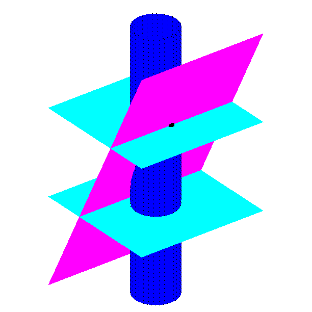
Figure 5: Illustration of the propagation and reflection of singularities in pseudo-spacetime. Consider the conductivity $\sigma(x)=1+\chi_{B(0,r_{0})}(x)$. The dark blue pillar is a vertical cylinder whose base is the singular support of $\mu$, here $\partial B(0,r_{0})$. For fixed $\varphi$, the map $(x,t)\mapsto\widehat{v}_{1}(x,t,e^{i\varphi})$ is singular on three planes. The magenta plane is the singular support of the incident wave $\rho_{\varphi}(x,t)=c\delta^{\prime}(t+2\text{Re}\,(e^{i\varphi}x))$. We have $\widehat{v}_{1}(x,t,e^{i\varphi})=\overline{\partial}^{-1}_{x}(\mu\,\cdotp\rho_{\varphi})$ where $\overline{\partial}^{-1}_{x}$ propagates the singularities of the product $\mu\,\cdotp\rho_{\varphi}$ in the light-blue horizontal planes $t=2r_{0}$ and $t=-2r_{0}$.

Connecting the Radon Transform and the Conductivity Equation

The propagation of certain types of oscillations in the solutions of the conductivity equation is analyzed in detail in [18] using microlocal analysis and so-called complex principal-type operators, introduced by Duistermaat and Hörmander [15]. More precisely, it is shown in Greenleaf et al. [18] that the conductivity equation may be transformed to an equation of which the principal part is the complex derivative $\overline{\partial}_{x}$, by conjugating the equation with (i) operators of multiplication by a complex exponential function, and (ii) appropriate Fourier integral operators. This implies that the oscillations in the solutions of the conductivity equation propagate along two-dimensional spaces in the suitable phase space and satisfy a relation involving the two-dimensional Radon transform. Below we will derive the relationship between the Radon transform and the conductivity equation in a simpler way, using only elementary complex analysis and the properties of the Fourier transform. To introduce the complex formulation of the conductivity equation we identify the real-valued coordinates $x=(x_{1},x_{2})\in{\mathbb{R}}^{2}$ with complex-valued points $x=x_{1}+ix_{2}\in{\mathbb{C}}$. We recall that the complex Wirtinger derivatives are

$$\overline{\partial}_{x}=\frac{1}{2}(\frac{\partial}{\partial x_{1}}+i\frac{\partial}{\partial x_{2}}),\quad\partial_{x}=\frac{1}{2}(\frac{\partial}{\partial x_{1}}-i\frac{\partial}{\partial x_{2}}),\quad x\in{\mathbb{C}}.$$

Let $k\in{\mathbb{C}}$ be the complex wave number, factored as $k=\tau\theta$ where $\tau\in{\mathbb{R}}$ and $\theta\in{\mathbb{C}}$, $|\theta|=1$. We call $\tau$ the complex frequency, and later we will introduce the pseudo-time variable $t$, which is the Fourier-domain variable corresponding to $\tau$.

The solution $u$ of the conductivity equation (4) can be written as

$$u(x)=\text{Re}\,\,(f_{\mu}(x))$$ (15)

where $f_{\mu}(x)$ is the solution of the Beltrami equation

$$\overline{\partial}_{x}f_{\mu}(x)=\mu(x)\,\overline{\partial_{x}f_{\mu}(x)},\quad x\in\mathbb{C}.$$

Until otherwise stated, we treat $x$ as a complex number $x=x_{1}+ix_{2}$. The representation (15) is analogous to the fact that any harmonic function can be written as the real part of an analytic function.

Moreover, Astala and Päivärinta [7] constructed unique complex geometrical optics (CGO) solutions for the Beltrami equation with specific asymptotics at infinity,

$$\overline{\partial}_{x}f_{\mu}(x,k) =\mu(x)\,\overline{\partial_{x}f_{\mu}(x,k)},\quad x\in{\mathbb{C}},$$ (16)

$$f_{\mu}(x,k) =e^{ikx}(1+{\mathcal{O}}(|x|^{-1}))\hbox{ as }|x|\to\infty,$$ (17)

which depend on ${x}$ and a complex wave number $k\in{\mathbb{C}}$. When $\sigma({x})$ is equal to 1 in the complement of the domain $\Omega$ and $0<c_{1}\leq\sigma({x})\leq c_{2}$, the Beltrami coefficient $\mu$ is supported in $\Omega$ and satisfies $\|\mu\|_{L^{\infty}({\mathbb{C}})}<1$. Using such solutions of the Beltrami equations, we will below consider the function

$$u(x,k)=\text{Re}\,\,(f_{\mu}(x,k))$$ (18)

which satisfies $\nabla_{x}\,\cdotp\sigma({x})\nabla_{x}u({x},k)=0$. It is shown in [7] that the map $\Lambda_{\sigma}:u|_{\partial\Omega}\to n\cdot\sigma\nabla u|_{\partial\Omega}$ determines the function $f_{\mu}(x,k)$ for $x\in{\mathbb{C}}\setminus\Omega$ and $k\in{\mathbb{C}}$. Let us write the CGO solutions of (16) in the form

$${f_{\mu}(x,k)=e^{ikx}v(x,k),}$$

$$v(x,k)=1+{v_{sc}(x,k),}$$

$$v_{sc}(x,k)={\mathcal{O}}(|x|^{-1}),\quad\hbox{as }x\to\infty.$$

Then, (16) yields

$$\overline{\partial}_{x}v_{sc}-e_{-k}\mu(\overline{\partial_{x}v_{sc}-ikv_{sc}})=-i\overline{k}e_{-k}\mu.$$

The solid Cauchy transform $\overline{\partial}_{x}^{-1}$ is the operator

$$\overline{\partial}_{x}^{-1}f(x) = \frac{1}{\pi}\int_{\mathbb{C}}\frac{1}{x-x^{\prime}}f(x^{\prime})\,d^{2}x^{\prime},$$ (19)

where $d^{2}x^{\prime}=dm(x^{\prime})$ is the Lebesgue measure of ${\mathbb{C}}={\mathbb{R}}^{2}$. Then, we see that $v_{sc}(x,k)$ satisfies

$$\big{(}I-\mathcal{A}\big{)}v_{sc}=-i\overline{k}\,\overline{\partial}_{x}^{-1}(e_{-k}\mu),$$

where $\mathcal{A}$ is the real-linear operator

$$\mathcal{A}:v\to\overline{\partial}_{x}^{-1}(e_{k}\mu\rho(\partial_{x}+ik)v)$$

and $\rho(f):=\overline{f}$ denotes complex conjugation. Using the equation $\big{(}I-\mathcal{A}\big{)}v_{sc}=-i\overline{k}\,\overline{\partial}_{x}^{-1}(e_{-k}\mu)$ and the Neumann series for $(I-\mathcal{A})^{-1}$, we can write formally (the discussion on the precise sense in which this series converges is omitted in this paper, see [18] for detailed analysis)

$$v_{sc}\sim\sum_{n=1}^{\infty}v_{n},\quad v_{1}=-i\overline{k}\,\overline{\partial}_{x}^{-1}(e_{-k}\mu),\quad v_{n+1}=\mathcal{A}v_{n}.$$ (20)

Next we consider the term corresponding to single scattering,

$${v_{1}=-i\overline{k}\,\overline{\partial}_{x}^{-1}(e_{-k}\mu).}$$

The Dirichlet-to-Neumann map $\Lambda_{\sigma}$ determines $v_{sc}(x,k)$ for ${x\in\partial\Omega}$. However, below we consider the properties of the first term $v_{1}(x,k)|_{x\in\partial\Omega}$ in the series (20). The higher-order terms $v_{n}(x,k)|_{x\in\partial\Omega,}\,n\geq 2$ contribute “multiple scattering,” which explain artifacts in numerics.

Next, we analyze the term $v_{1}(x,k)$ corresponding to the single-order scattering in the pseudo-time domain. To do this we decompose the complex wave number $k$ as $k=\tau\theta,$ where $\theta=e^{i\varphi}$. We use the Fourier transform of the function $w(x,\tau)$, that is,

$$\widehat{w}(x,t)={\cal F}_{\tau\to t}w(x,t)=\int_{\mathbb{R}}e^{-it\tau}w(x,\tau)\,d\tau.$$

For a function $f(x,t)$ that depends on the $x$ and $t$ variables, the formula (19) implies

$$\overline{\partial}_{x}^{-1}f(x,t) =\frac{1}{\pi}\int_{\mathbb{C}}\frac{1}{x-x^{\prime}}f(x^{\prime},t)\,d^{2}x^{\prime}$$

$$=\frac{1}{\pi}\int_{\mathbb{R}}\int_{\mathbb{C}}\delta(t-t^{\prime})\frac{1}{x-x^{\prime}}f(x^{\prime},t^{\prime})\,d^{2}x^{\prime}dt^{\prime}.$$

This means that $f(x,t)\to\overline{\partial}_{x}^{-1}f(x,t)$ operates in each $t=$constant plane independently of the values of $f(x,t)$ in the other planes.

Using the polar coordinates $k=\tau e^{i\varphi}$, we see for $w=w(x,\tau),$

$$e_{-k}w=e^{-2i\text{Re}\,(kx)}w(x,\tau)=e^{-2i\tau\text{Re}\,(e^{i\varphi}x)}w(x,\tau).$$

Thus, it holds for the Fourier transform that

$$\widehat{\varepsilon_{-k}w}(x,t) = {\cal F}_{\tau\to t}(e_{-k}w)(x,t)$$

$$= \int_{\mathbb{R}}e^{-it\tau}e^{-2i\tau\text{Re}\,(e^{i\varphi}x)}w(x,\tau)\,d\tau$$

$$= \widehat{w}(x,t+2\text{Re}\,(e^{i\varphi}x)).$$

This can we viewed as ‘tilting’ the $\{t=0\}$ plane in the space ${\mathbb{C}}\times{\mathbb{R}}$, having the coordinates $(x,\tau)$, by using the operation $(x,\tau)\to(x,t+2\text{Re}\,(e^{i\varphi}x)).$

As the Fourier transform of $\mu(x,\tau)=\mu(x)=\mu(x){\bf 1}(\tau)$ is $\widehat{\mu}(x,t)=\mu(x)\delta(\tau)$, we see that

$${\cal F}_{\tau\to t}(e_{-k}\mu)(x,t) = \delta(t+2\text{Re}\,(e^{i\varphi}x))\mu(x).$$

Thus, the Fourier transform of the single scattering term

$$v_{1}(x,t,e^{i\varphi})=-i\overline{k}\,\overline{\partial}_{x}^{-1}(e_{-k}\mu)$$

is equal to

$$\widehat{v}_{1}(x,t,e^{i\varphi})=2e^{-i\varphi}\int_{{\mathbb{C}}}\frac{1}{x-x^{\prime}}\,{\delta^{\prime}(t+2\text{Re}\,(e^{i\varphi}x^{\prime}))}\mu(x^{\prime})\,d^{2}x^{\prime}.$$

Due to this, we define the linear operator $T_{1}$ that maps a compactly supported function $\mu(x^{\prime})$ in $\Omega$ to the corresponding single scattering term $\widehat{v}_{1}$,

$$\mu(x^{\prime})\mapsto(T_{1}\mu)(x,t,e^{i\varphi})=\widehat{v}_{1}(x,t,e^{i\varphi}).$$

The Schwartz kernel of $T_{1}$ is

$$K_{1}(x,t,e^{i\varphi},x^{\prime})=\Big{(}\frac{2e^{-i\varphi}}{x-x^{\prime}}\Big{)}\delta^{\prime}(t+2\text{Re}\,(e^{i\varphi}x^{\prime})),$$

that is,

$$(T_{1}\mu)(x,t,e^{i\varphi})=\frac{\partial}{\partial t}\int_{\mathbb{C}}\frac{2e^{-i\varphi}}{x-x^{\prime}}\delta(t+2\text{Re}\,(e^{i\varphi}x^{\prime}))\mu(x^{\prime})d^{2}x^{\prime}.$$

Next, we aim to introduce a filtered back-projection formula. To this end, let us consider the ‘complex average’ of $\widehat{v}_{1}(x,t,e^{i\varphi})$ over $x\in\partial\Omega$,

$$\widehat{v}_{1}^{a}(t,e^{i\varphi})=\frac{1}{2\pi i}\int_{\partial\Omega}\widehat{v}_{1}(x,t,e^{i\varphi}){dx.}$$

Let $T_{1}^{a}$ be the linear operator $T_{1}^{a}:\mu\mapsto\widehat{v}_{1}^{a}$. That is,

$$(T_{1}^{a}\mu)(t,e^{i\varphi})=\frac{\partial}{\partial t}\int_{\mathbb{C}}2e^{-i\varphi}\delta(t+2\text{Re}\,(e^{i\varphi}x^{\prime}))\mu(x^{\prime})d^{2}x^{\prime},$$

which we obtain by using the Cauchy theorem and the fact that that $x^{\prime}\in\Omega$, so that

$$\frac{1}{2\pi i}\int_{\partial\Omega}\frac{2}{x-x^{\prime}}dx=\frac{1}{2\pi i}\int_{\partial\Omega}\frac{2}{\frac{x}{x^{\prime}}-1}\frac{1}{x^{\prime}}dx=\frac{1}{2\pi i}\int_{\{x^{\prime\prime}=x/x^{\prime}:\ x\in\partial\Omega\}}\frac{2}{x^{\prime\prime}-1}dx^{\prime\prime}=2.$$

We observe that $T_{1}^{a}$ is a generalized Radon transform: When we denote $n_{\varphi}=(\cos({\varphi}),\sin({\varphi}))\in{\mathbb{R}}^{2}$ we have

$$\text{Re}\,(e^{i\varphi}x)=n_{-\varphi}\cdot{x},$$ (21)

with $x=x_{1}+ix_{2}$ in the left hand side and $x=(x_{1},x_{2})$ in the right hand side. In what follows, we continue to consider $x$ as a vector in ${\mathbb{R}}^{2}$. Then

$$(T_{1}^{a}\mu)(t,e^{i\varphi})=2e^{-i\varphi}\frac{\partial}{\partial t}\int_{{\mathbb{R}}^{2}}\delta(t+2n_{-\varphi}\cdot{x})\mu({x})d{x}=e^{-i\varphi}\frac{\partial}{\partial t}{\mathcal{R}}\mu({-\varphi},\frac{1}{2}t),$$

where

$${\mathcal{R}}\mu({\varphi},s)=\int_{n_{\varphi}\cdot{x}=s}\mu({x})d\ell({x})$$

is the 2-dimensional Radon transform of the function $\mu$ and $d\ell$ is the length measure on a line.

The filtered back-projection formula in [30] for the inverse Radon transform leads to the following theorem (for a detailed proof, see [18]).

Theorem 0.1.

The operator $(T_{1}^{a})^{*}T_{1}^{a}$ is a pseudo-differential operator of order $1$ with

$$\sigma_{\mbox{\tiny prin}}((T_{1}^{a})^{*}T_{1}^{a})(x,\zeta)=2\pi^{2}|\zeta|,\quad x\in\Omega,\ \zeta\in{\mathbb{R}}^{2}\setminus 0,$$

where $\sigma_{\mbox{\tiny prin}}$ stands for the principal symbol, and

$$\frac{1}{2\pi^{2}}(-\Delta)^{-\frac{1}{2}}(T_{1}^{a})^{*}T_{1}^{a}=I+K,$$ (22)

where $K$ is a smoothing integral operator (a pseudo-differential operator of order $-1$).

Formula (22) provides a reconstruction formula for the function $\mu$, and therefore for $\sigma$, which is analogous to the filtered back-projection formula for the Radon transform.

References

- [1] Juan Pablo Agnelli, Aynur Cöl, Matti Lassas, Rashmi Murthy, Matteo Santacesaria, and Samuli Siltanen. Classification of stroke using neural networks in electrical impedance tomography. Inverse Problems, 36(11):115008, 2020.
- [2] Giovanni Alessandrini. Stable determination of conductivity by boundary measurements. Applicable Analysis, 27(1-3):153–172, 1988.
- [3] Melody Alsaker and Jennifer L Mueller. A d-bar algorithm with a priori information for 2-dimensional electrical impedance tomography. SIAM Journal on Imaging Sciences, 9(4):1619–1654, 2016.
- [4] Melody Alsaker, Siiri Rautio, and Samuli Siltanen. VHPT with TV reconstruction: a software package for regularized virtual hybrid parallel-beam tomography (v1.0), Zenodo. https://zenodo.org/records/12581354, 2024.
- [5] James Ambrose. Computerized transverse axial scanning (tomography): Part 2. clinical application. The British journal of radiology, 46(552):1023–1047, 1973.
- [6] Kari Astala, Jennifer L Mueller, Lassi Päivärinta, Allan Perämäki, and Samuli Siltanen. Direct electrical impedance tomography for nonsmooth conductivities. Inverse Problems and Imaging, 5(3):531–549, 2011.
- [7] Kari Astala and Lassi Päivärinta. A boundary integral equation for calderón’s inverse conductivity problem. Collectanea Mathematica, page 127–139, 2006.
- [8] Benoit Brazey, Yassine Haddab, and Nabil Zemiti. Robust imaging using electrical impedance tomography: review of current tools. Proceedings of the Royal Society A, 478(2258):20210713, 2022.
- [9] Kristian Bredies. Recovering piecewise smooth multichannel images by minimization of convex functionals with total generalized variation penalty. In Efficient Algorithms for Global Optimization Methods in Computer Vision: International Dagstuhl Seminar, Dagstuhl Castle, Germany, November 20-25, 2011, Revised Selected Papers, page 44–77. Springer, 2014.
- [10] Brian H Brown and Andrew D Seagar. The sheffield data collection system. Clinical physics and physiological measurement, 8(4A):91–97, 1987.
- [11] Peter Caday, Maarten V. de Hoop, Vitaly Katsnelson, and Gunther Uhlmann. Scattering control for the wave equation with unknown wave speed. Arch. Ration. Mech. Anal., 231(1):409–464, 2019.
- [12] A.-P. Calderón. On an inverse boundary value problem. In Seminar on Numerical Analysis and its Applications to Continuum Physics (Rio de Janeiro, 1980), page 65–73. Soc. Brasil. Mat., Rio de Janeiro, 1980.
- [13] Kuo-Sheng Cheng, David Isaacson, JC Newell, and David G Gisser. Electrode models for electric current computed tomography. IEEE Transactions on Biomedical Engineering, 36(9):918–924, 1989.
- [14] Thiago de Castro Martins, André Kubagawa Sato, Fernando Silva de Moura, Erick Dario León Bueno de Camargo, Olavo Luppi Silva, Talles Batista Rattis Santos, Zhanqi Zhao, Knut Möeller, Marcelo Brito Passos Amato, Jennifer L. Mueller, Raul Gonzalez Lima, and Marcos de Sales Guerra Tsuzuki. A review of electrical impedance tomography in lung applications: Theory and algorithms for absolute images. Annual Reviews in Control, 48:442–471, 2019.
- [15] J. J. Duistermaat and L. Hörmander. Fourier integral operators. II. Acta Math., 128(3-4):183–269, 1972.
- [16] L. D. Faddeev. Increasing solutions of the Schrödinger equation. Soviet Physics Doklady, 10:1033–1035, 1966.
- [17] Henrik Garde and Nuutti Hyvönen. Mimicking relative continuum measurements by electrode data in two-dimensional electrical impedance tomography. Numerische Mathematik, 147:579–609, 2021.
- [18] Allan Greenleaf, Matti Lassas, Matteo Santacesaria, Samuli Siltanen, and Gunther Uhlmann. Propagation and recovery of singularities in the inverse conductivity problem. Analysis & PDE, 11(8):1901–1943, 2018.
- [19] Allan Greenleaf and Gunther Uhlmann. Nonlocal inversion formulas for the X-ray transform. Duke Math. J., 58(1):205–240, 1989.
- [20] S. J. Hamilton and A. Hauptmann. Deep d-bar: Real-time electrical impedance tomography imaging with deep neural networks. IEEE Transactions on Medical Imaging, 37(10):2367–2377, 2018.
- [21] Godfrey N Hounsfield. Computerized transverse axial scanning (tomography): Part 1. description of system. The British journal of radiology, 46(552):1016–1022, 1973.
- [22] David Isaacson, Jennifer L Mueller, Jonathan C Newell, and Samuli Siltanen. Reconstructions of chest phantoms by the d-bar method for electrical impedance tomography. IEEE Transactions on medical imaging, 23(7):821–828, 2004.
- [23] Annemijn H. Jonkman, Glasiele C. Alcala, Bertrand Pavlovsky, Oriol Roca, Savino Spadaro, Gaetano Scaramuzzo, Lu Chen, Jose Dianti, Mayson L. de A. Sousa, Michael C. Sklar, Thomas Piraino, Huiqing Ge, Guang-Qiang Chen, Jian-Xin Zhou, Jie Li, Ewan C. Goligher, Eduardo Costa, Jordi Mancebo, Tommaso Mauri, Marcelo Amato, Laurent J. Brochard, Tobias Becher, Giacomo Bellani, Francois Beloncle, Gilda Cinnella, Carla Fornari, Inéz Frerichs, Claude Guerin, Ahmed Mady, Fabiana Madotto, Alain Mercat, Ibrahim Nagwa, Stefano Nava, Paolo Navalesi, Elena Spinelli, and Daniel Talmor. Lung recruitment assessed by electrical impedance tomography (recruit): A multicenter study of covid-19 acute respiratory distress syndrome. American Journal of Respiratory and Critical Care Medicine, 208(1):25–38, 2023.
- [24] Diederik P Kingma and Jimmy Ba. Adam: A method for stochastic optimization. arXiv preprint arXiv:1412.6980, 2014.
- [25] Kim Knudsen, Matti Lassas, Jennifer L Mueller, and Samuli Siltanen. Regularized d-bar method for the inverse conductivity problem. Inverse Problems and Imaging, 35(4):599–624, 2009.
- [26] James Clerk Maxwell. Viii. a dynamical theory of the electromagnetic field. Philosophical transactions of the Royal Society of London, 155:459–512, 1865.
- [27] Jennifer L Mueller. Evaluation of pulmonary structure and function in patients with cystic fibrosis from electrical impedance tomography data. Biomedical Engineering Technologies: Volume 1, 1:733–750, 2022.
- [28] Jennifer L Mueller and Samuli Siltanen. Linear and nonlinear inverse problems with practical applications. SIAM, 2012.
- [29] Adrian I. Nachman. Global uniqueness for a two-dimensional inverse boundary value problem. Annals of Mathematics, 143(1):71–96, 1996.
- [30] Frank Natterer. Computerized tomography. Springer, 1986.
- [31] François Perier, Samuel Tuffet, Tommaso Maraffi, Glasiele Alcala, Marcus Victor, Anne-Fleur Haudebourg, Keyvan Razazi, Nicolas De Prost, Marcelo Amato, Guillaume Carteaux, et al. Electrical impedance tomography to titrate positive end-expiratory pressure in covid-19 acute respiratory distress syndrome. Critical Care, 24:1–9, 2020.
- [32] Robert L Powell. Experimental techniques for multiphase flows. Physics of fluids, 20(4), 2008.
- [33] Johann Radon. Uber die bestimmung von funktionen durch ihre integralwerte langs gewissez mannigfaltigheiten, ber. Verh. Sachs. Akad. Wiss. Leipzig, Math Phys Klass, 69, 1917.
- [34] Olaf Ronneberger, Philipp Fischer, and Thomas Brox. U-net: Convolutional networks for biomedical image segmentation. In Medical Image Computing and Computer-Assisted Intervention–MICCAI 2015: 18th International Conference, Munich, Germany, October 5-9, 2015, Proceedings, Part III 18, page 234–241. Springer, 2015.
- [35] Wilhelm Conrad Röntgen. On a new kind of rays. Science, 3(59):227–231, 1896.
- [36] Leonid I Rudin, Stanley Osher, and Emad Fatemi. Nonlinear total variation based noise removal algorithms. Physica D: nonlinear phenomena, 60(1-4):259–268, 1992.
- [37] Talles Batista Rattis Santos, Rafael Mikio Nakanishi, Jari P Kaipio, Jennifer L Mueller, and Raul Gonzalez Lima. Introduction of sample based prior into the d-bar method through a schur complement property. IEEE transactions on medical imaging, 39(12):4085–4093, 2020.
- [38] Omid Rajabi Shishvan, Ahmed Abdelwahab, Nilton Barbosa da Rosa, Gary J. Saulnier, Jennifer L. Mueller, Jonathan C. Newell, and David Isaacson. Act5 electrical impedance tomography system. IEEE Transactions on Biomedical Engineering, 71(1):227–236, 2024.
- [39] Emil Y Sidky and Xiaochuan Pan. Image reconstruction in circular cone-beam computed tomography by constrained, total-variation minimization. Physics in Medicine & Biology, 53(17):4777–4807, 2008.
- [40] Samuli Siltanen, Jennifer Mueller, and David Isaacson. An implementation of the reconstruction algorithm of a nachman for the 2d inverse conductivity problem. Inverse Problems, 16(3):681–699, 2000.
- [41] Erkki Somersalo, Margaret Cheney, and David Isaacson. Existence and uniqueness for electrode models for electric current computed tomography. SIAM Journal on Applied Mathematics, 52(4):1023–1040, 1992.
- [42] DR Stephenson, R Mann, and TA York. The sensitivity of reconstructed images and process engineering metrics to key choices in practical electrical impedance tomography. Measurement Science and Technology, 19(9):094013, 2008.
- [43] John Sylvester and Gunther Uhlmann. A global uniqueness theorem for an inverse boundary value problem. Annals of mathematics, page 153–169, 1987.
- [44] Philip van der Zee, Peter Somhorst, Henrik Endeman, and Diederik Gommers. Electrical impedance tomography for positive end-expiratory pressure titration in covid-19–related acute respiratory distress syndrome. American Journal of Respiratory and Critical Care Medicine, 202(2):280–284, 2020.