SUMO: Search-Based Uncertainty Estimation for Model-Based Offline Reinforcement Learning

Abstract

The performance of offline reinforcement learning (RL) suffers from the limited size and quality of static datasets. Model-based offline RL addresses this issue by generating synthetic samples through a dynamics model to enhance overall performance. To evaluate the reliability of the generated samples, uncertainty estimation methods are often employed. However, model ensemble, the most commonly used uncertainty estimation method, is not always the best choice. In this paper, we propose a Search-based Uncertainty estimation method for Model-based Offline RL (SUMO) as an alternative. SUMO characterizes the uncertainty of synthetic samples by measuring their cross entropy against the in-distribution dataset samples, and uses an efficient search-based method for implementation. In this way, SUMO can achieve trustworthy uncertainty estimation. We integrate SUMO into several model-based offline RL algorithms including MOPO and Adapted MOReL (AMOReL), and provide theoretical analysis for them. Extensive experimental results on D4RL datasets demonstrate that SUMO can provide more accurate uncertainty estimation and boost the performance of base algorithms. These indicate that SUMO could be a better uncertainty estimator for model-based offline RL when used in either reward penalty or trajectory truncation. Our code is available and will be open-source for further research and development.

Introduction

Offline reinforcement learning (RL) (Levine et al. 2020; Prudencio, Maximo, and Colombini 2023) aims to learn the optimal policy from a static dataset collected in advance, avoiding the risks and costs associated with environmental interaction in typical RL (Sutton and Barto 2018). Nevertheless, since the datasets cannot cover the entire state-action space, the offline agent cannot accurately estimate the Q-value for out-of-distribution (OOD) samples, ultimately leading to a degradation in the agent’s performance.

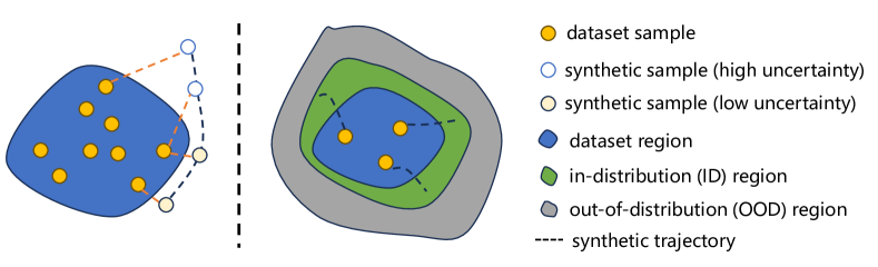
Figure 1: Left: The key idea of SUMO. For a synthetic sample, we calculate its KNN distance within the dataset as the uncertainty estimation. Right: An example of combining SUMO with AMOReL for trajectory truncation. Thanks to the accurate uncertainty estimation provided by SUMO, the agent can explore ID regions while avoiding OOD regions.

Model-based offline RL (Yu et al. 2020, 2021; Kidambi et al. 2020) employs a promising idea to address OOD issues. By leveraging an environmental dynamics model obtained by supervised learning, the agent can collect samples within the dynamics model and train the policy using these samples. This significantly enhances the performance and generalization of the agent. However, synthetic samples generated by the dynamics model may not be reliable (Lyu, Li, and Lu 2022), as the dynamics model’s reliability in OOD regions is not guaranteed. Training the policy with unreliable samples can lead to a performance decline. Therefore, evaluating the reliability of generated samples is critical. It is common to assess the reliability with uncertainty estimation (Lockwood and Si 2022; An et al. 2021). Current model-based offline RL methods often employ model ensemble-based techniques for uncertainty estimation, such as max aleatoric (Yu et al. 2020) and max pairwise diff (Kidambi et al. 2020). Subsequently, the estimated uncertainty can be used for trajectory truncation (Kidambi et al. 2020; Zhang et al. 2023b) or reward penalties (Yu et al. 2020) to mitigate OOD issues. However, model ensemble-based uncertainty estimation methods may be unreliable (Yu et al. 2021) because the models can be poorly learned, making their uncertainty estimation questionable. We wonder: Can we design a better uncertainty estimation method for model-based offline RL?

In this paper, we propose a Search-based Uncertainty estimation method for Model-based Offline RL (SUMO). SUMO characterizes the uncertainty of synthetic samples as the cross entropy between model dynamics and true dynamics, which can be shown as a more reasonable uncertainty estimation than model ensemble-based estimation. Moreover, the estimated uncertainty for a given sample does not involve extra training of neural networks. In contrast, the uncertainty estimated by model ensemble methods is correlated with the training process and training data distribution since they need to train dynamics models parameterized by neural networks. To estimate the cross entropy practically, we employ a particle-based entropy estimator (Singh et al. 2003), transforming the problem into a $k$-nearest neighbor (KNN) search problem, as shown in Figure 1 (left), that is the reason we call SUMO a search-based method. Furthermore, given the large search space and high data dimensionality, we employ FAISS (Johnson, Douze, and Jégou 2019) to ensure efficient KNN search. We note that SUMO is algorithm-agnostic, allowing us to integrate it with any model-based offline RL algorithm which needs uncertainty estimation. For instance, it can be combined with MOPO (Yu et al. 2020) or with Adapted MOReL (Kidambi et al. 2020) (AMOReL, which we discuss in later sections), as shown in Figure 1 (right).

We integrate SUMO with several off-the-shelf model-based offline RL algorithms like MOPO and AMOReL and theoretically analyze their performance bounds after introducing SUMO. Empirically, we conduct extensive experiments on the D4RL (Fu et al. 2020) benchmark, and the experimental results indicate that SUMO can significantly enhance the performance of base algorithms. We also show that SUMO can provide more accurate uncertainty estimation than commonly used model ensemble-based methods. Our contributions can be summarized as follows:

• We propose a novel search-based uncertainty estimation method for model-based offline RL, SUMO.

• We combine SUMO with AMOReL and MOPO, and provide theoretical performance bounds.

• We empirically demonstrate that SUMO incurs accurate uncertainty estimation and can bring significant performance improvement over the base algorithms on numerous D4RL datasets.

Background

Reinforcement Learning (RL). We consider a Markov Decision Process (MDP) (Garcia and Rachelson 2013) modeled by $\mathcal{M}=\langle S,A,r,P,\rho,\gamma\rangle$, where $S$ is the state space, $A$ is the action space, $r$ is the reward function: $S\times A\rightarrow\mathbb{R}$, $P$ is the transition dynamics: $S\times A\times S\rightarrow[0,1]$, $\rho$ is the initial state distribution, and $\gamma\in[0,1)$ is the discount factor. RL aims to get a policy $\pi_{\theta}(a|s)$ that maximizes the cumulative expected discounted return: $J_{\rho}(\pi,\mathcal{M})=\max_{\pi_{\theta}}\mathbb{E}_{\pi_{\theta}}\left[\sum_{t=0}^{\infty}\gamma^{t}r(s_{t},a_{t})|s_{0}\sim\rho\right]$. We specify $\mathcal{M}$ to stress that $J_{\rho}(\pi,\mathcal{M})$ is obtained in the MDP $\mathcal{M}$.

Offline RL. In offline RL, the agent aims to learn the optimal batch-constraint policy based on a static dataset $\mathcal{D}=\{(s_{i},a_{i},r_{i},s_{i+1})\}_{i=1}^{N}$, where the samples are collected by a (unknown) behavior policy $\mu$, without accessing the environment. Since the dataset can not cover the entire state-action space, the performance of offline RL is often limited.

Model-based Offline RL. Model-based offline RL leverages the learned dynamics model $P_{\widehat{\mathcal{M}}}(\cdot|s,a)$ to generate synthetic samples. This allows us to train the policy using both dataset transitions and samples generated by the dynamics model. We denote the model MDP as $\widehat{\mathcal{M}}$, the state distribution probability at timestep $t$ following policy $\pi$ and dynamics $P_{\widehat{\mathcal{M}}}$ as $\mathbb{P}_{\widehat{\mathcal{M}},t}^{\pi}(s)$, and discounted occupancy measure of $\pi$ under dynamics $P_{\widehat{\mathcal{M}}}$ as $\hat{\rho}^{\pi}(s,a):=\pi(a|s)\sum_{t=0}^{\infty}\gamma^{t}\mathbb{P}_{\widehat{\mathcal{M}},t}^{\pi}(s)$.

Related Work

Model-free Offline RL. Model-free offline RL aims to train an agent merely on a static dataset without a dynamics model. The major challenge for model-free offline RL is extrapolation error (Fujimoto, Meger, and Precup 2019; Kumar et al. 2020; Lyu et al. 2022) of the Q-function due to the inability to explore. Existing methods introduce conservatism to the policy (Fujimoto and Gu 2021; Kumar et al. 2019; Fujimoto, Meger, and Precup 2019) or Q-function (Kumar et al. 2020; Lyu et al. 2022; An et al. 2021; Yang et al. 2024) to tackle the issue. However, the involvement of conservatism restricts the generalization ability of the policy.

Model-based Offline RL. Model-based offline RL leverages a dynamics model to extend the dataset and enhance the generalization ability. Since the dynamics model may not be accurate on all transitions, conservatism is still necessary for learning a good policy. Some works (Yu et al. 2020; Kidambi et al. 2020) incorporate conservatism into the generated samples, while other works (Yu et al. 2021; Rigter, Lacerda, and Hawes 2022; Liu et al. 2023) introduce conservatism to Q-function.

Uncertainty Estimation in offline RL. In model-free offline RL, uncertainty measures the distance of samples from the dataset distribution. EDAC (An et al. 2021) leverages an ensemble of Q-networks to estimate the uncertainty. DARL (Zhang et al. 2023a) computes the KNN distances between the samples and the dataset as uncertainty estimation. In model-based offline RL, uncertainty measures the discrepancy between the simulated dynamics and the true dynamics. MOPO (Yu et al. 2020) and MOReL (Kidambi et al. 2020) estimate the uncertainty by model ensemble. MOBILE (Sun et al. 2023) quantifies the uncertainty through model-bellman inconsistency. All of these uncertainty estimation methods rely on model ensemble, while our method does not. Some other uncertainty estimation methods (Kim and Oh 2023; Tennenholtz and Mannor 2022) suffer from heavy computational burden and complex implementation, while our method is both efficient and easy to implement.

Methodology

Search-based method for Uncertainty Estimation

In this part, we formally present our search-based uncertainty estimation method for model-based offline RL. Firstly, we outline how we model the uncertainty estimation problem as an estimation of cross entropy. Subsequently, we employ a particle-based entropy estimator, which approximates the calculation of cross entropy as a search problem.

We characterize the uncertainty of the model dynamics as its cross entropy against the true dynamics: $\mathcal{H}(P_{\widehat{\mathcal{M}}}(\cdot|s,a),P(\cdot|s,a))=-\sum P_{\widehat{\mathcal{M}}}(\cdot|s,a)\log P(\cdot|s,a)$, where $P_{\widehat{\mathcal{M}}}(\cdot|s,a)$ and $P(\cdot|s,a)$ are the model dynamics and the true dynamics, respectively. It is hard to calculate $\mathcal{H}(P_{\widehat{\mathcal{M}}}(\cdot|s,a),P(\cdot|s,a))$ since we have no knowledge about the true dynamics $P(\cdot|s,a)$. We therefore compute the cross entropy between the model dynamics and the dataset dynamics: $\mathcal{H}(P_{\widehat{\mathcal{M}}}(\cdot|s,a),P_{d}(\cdot|s,a))=-\sum P_{\widehat{\mathcal{M}}}(\cdot|s,a)\log P_{d}(\cdot|s,a)$, where $P_{d}(\cdot|s,a)$ denotes the dataset transition dynamics of dataset MDP, which is formally defined below.

Definition 1 (dataset MDP).

The dataset MDP is defined by the tuple $\hat{\mathcal{M}_{d}}=(S,A,r,P_{d},\rho_{d},\gamma)$, where $S$, $A$, $r$ and $\gamma$ are the same as the original MDP. The dataset transition dynamics $P_{d}$ is defined as:

$$P_{d}(\cdot|s,a)=\begin{cases}P(\cdot|s,a),\qquad\mathrm{if}\,(s,a)\in\mathcal{D},\\ 0,\qquad\qquad\qquad\mathrm{otherwise,}\end{cases}$$ (1)

and $\rho_{d}$ is the state distribution of the dataset.

Remark: Intuitively, $P_{d}$ only accounts for transitions that lie in the dataset; we set the probability for transitions not in the dataset to be zero. Note that the summation of $P_{d}$ for a given state-action pair $(s,a)$ may be not 1, we can scale $P_{d}$ accordingly to make it a valid probability density function.

Then based on the definition of cross entropy, we have $\mathcal{H}(P_{\widehat{\mathcal{M}}},P_{d})=-\frac{1}{n}\sum_{i=1}^{n}\log P_{d}(x_{i})$, where $\{x_{i}\}_{i=1}^{n}\sim P_{\widehat{\mathcal{M}}}$. According to the particle-based entropy estimator (Singh et al. 2003), given a dataset $\{y_{j}\}_{j=1}^{m}\sim P_{d}$, we have $P_{d}(x_{i})=\frac{k\Gamma(d/2+1)}{m\pi^{d/2}R_{i,k,m}^{d}}$, where $d$ is the dimension of $x_{i}$, $\Gamma$ is the Gamma function, and $R_{i,k,m}^{d}=\|x_{i}-x_{i}^{k,m}\|_{2}^{d}$ represents the distance between $x_{i}$ and the $k$-nearest neighbor of $x_{i}$ in $\{y_{j}\}_{j=1}^{m}$. Then, we can compute the cross entropy as:

$$\begin{split}\mathcal{H}(P_{\widehat{\mathcal{M}}},P_{d})&=-\frac{1}{n}\sum_{i=1}^{n}\log\frac{k\Gamma(d/2+1)}{m\pi^{d/2}R_{i,k,m}^{d}}\\ &\propto\frac{1}{n}\sum_{i=1}^{n}\log\|x_{i}-x_{i}^{k,m}\|_{2}\end{split}$$ (2)

Notice that Equation (2) is an uncertainty estimation of the model dynamics. To estimate the uncertainty of a sample $x_{i}$ generated by the dynamics model, we can assume $P_{\widehat{\mathcal{M}}}$ is a delta distribution, where $P_{\widehat{\mathcal{M}}}(x_{i})=\infty$, $P_{\widehat{\mathcal{M}}}(x)=0$ for any $x\neq x_{i}$. Thus, we transform the problem of estimating the uncertainty of synthetic samples into a KNN search problem. To be specific, given an offline dataset $\mathcal{D}=\{(s_{i},a_{i},r_{i},s_{i+1})\}_{i=1}^{N}$ and a synthetic sample $(\hat{s},\hat{a},\hat{r},\hat{s}^{\prime})$, we can estimate the uncertainty of the synthetic sample as:

$$u(\hat{s},\hat{a},\hat{s}^{\prime})=\log\left(\|(\hat{s}\oplus\hat{a}\oplus\hat{s}^{\prime})-(\hat{s}\oplus\hat{a}\oplus\hat{s}^{\prime})^{k,N}\|_{2}\right)$$ (3)

where $\oplus$ is the vector concatenation operator, $(\hat{s}\oplus\hat{a}\oplus\hat{s}^{\prime})^{k,N}$ returns the nearest neighbor of the query sample $(\hat{s},\hat{a},\hat{r},\hat{s}^{\prime})$ in the offline dataset, $k$ is the number of neighbors for KNN search, and $N$ is the number of samples in the dataset. To ensure the estimated uncertainty is non-negative, we practically compute the uncertainty as:

$$u(\hat{s},\hat{a},\hat{s}^{\prime})=\log\left(\|(\hat{s}\oplus\hat{a}\oplus\hat{s}^{\prime})-(\hat{s}\oplus\hat{a}\oplus\hat{s}^{\prime})^{k,N}\|_{2}+1\right)$$ (4)

Note that one can also involve the rewards in Equation (4) for computing the uncertainty, which we empirically do not find obvious performance difference in Appendix D.3. To ensure time efficiency, we employ FAISS (Johnson, Douze, and Jégou 2019), an efficient GPU-based KNN search method to estimate the uncertainty. Note that using KNN search to calculate distances between given samples and datasets is a widely used approach in model-free offline RL (Zhang et al. 2023a; Ran et al. 2023; Lyu et al. 2024). However, they often rely on constraining the distance between the learned policy and the behavior policy, and the concatenated vector only includes dimensions of $s$ and $a$. In contrast, for model-based offline RL, what matters is the discrepancy between the model dynamics and the true dynamics. Therefore, we need to consider the influence of $s^{\prime}$.

We then discuss the advantage of SUMO compared with model ensemble-based methods. First, SUMO estimates the uncertainty in an unsupervised learning manner, meaning that the estimated uncertainty is stable and not correlated with the training process. Second, model ensemble-based uncertainty estimation is an empirical approximation. A mismatch can be observed in theoretical analysis of prior works, e.g., $D_{TV}(P_{\widehat{\mathcal{M}}}(\cdot|s,a),P(\cdot|s,a))\leq\alpha$ is required in MOReL, where $D_{TV}$ is the total variation distance and $\alpha$ is the threshold. Model ensemble-based uncertainty estimation can only practically approximate the bound of $D_{TV}$ with $u$. In contrast, SUMO provides an unbiased estimate of cross entropy, relationships between $u$ and $D_{TV}$ can be established using Pinsker’s inequality (Csiszár and Körner 2011), as shown in Appendix A.2.

Integrating SUMO into Existing Methods

As an uncertainty estimation method, SUMO is compatible with any model-based offline RL algorithm that requires an estimation of uncertainty. There are two typical ways of using uncertainty in model-based offline RL, using the uncertainty as the reward penalty, e.g., MOPO (Yu et al. 2020), and using the uncertainty to truncate synthetic trajectories from the learned model, e.g., MOReL (Kidambi et al. 2020). In this part, we introduce the procedure of combining SUMO with MOPO and Adapted MOReL, respectively.

MOPO with SUMO

MOPO adopts the uncertainty as the reward penalty, and we can simply replace the uncertainty estimator as the SUMO estimator. The detailed pseudocode of MOPO+SUMO can be found in Appendix B, and the detailed process can summarized as:

Step1: Learning the Environmental Dynamics Model: We first construct an environmental dynamics model to simulate the true dynamics. Following previous works (Yu et al. 2020; Kidambi et al. 2020), we model the dynamics model as a multi-layer neural network which outputs a Gaussian distribution over the next state and reward: $\hat{P}_{\psi}(s^{\prime},r|s,a)=\mathcal{N}\left(\mu_{\psi}(s,a),\Sigma_{\psi}(s,a)\right)$. We use an ensemble dynamics model which consists of $N$ ensemble members: $\hat{P}_{\psi}=\{\hat{P}_{\psi_{i}}\}_{i=1}^{N}$. Note that we use the ensemble dynamics model solely to reduce the error in model predictions, not for estimating the uncertainty. Then we can train each ensemble member via maximum log-likelihood:

$$\mathcal{L}_{\psi_{i}}=\mathbb{E}_{(s,a,r,s^{\prime})\sim\mathcal{D}}\left[-\log\hat{P}_{\psi_{i}}(s^{\prime},r|s,a)\right]$$ (5)

Step2: Reward Penalty Calculation with SUMO: We utilize the current policy $\pi$ and the dynamics model $\hat{P}_{\psi}$ to generate synthetic samples. For each generated sample $(s,a,s^{\prime})$, we first calculate its unnormalized uncertainty with SUMO via Equation (4). We assume that the reward function satisfies: $0\leq r(s,a)\leq r_{max},\forall(s,a)$. This is easy to achieve in practice. Then we normalize $u(s,a,s^{\prime})$ to the range $[0,r_{max}]$:

$$\hat{u}(s,a,s^{\prime})=\frac{u(s,a,s^{\prime})}{\max_{(s,a,s^{\prime})}u(s,a,s^{\prime})}\times r_{max}$$ (6)

We adopt $\hat{u}$ to penalize the rewards, $\hat{r}=r-\lambda\hat{u}$, where $\lambda$ is a hyperparameter that controls the magnitude of the penalty. We can then add the synthetic samples with reward penalty to the synthetic dataset $\mathcal{D}_{model}$.

Step 3: Model-based Policy Optimization: We then follow MOPO to train SAC (Haarnoja et al. 2018) agent with samples drawn from the offline dataset $\mathcal{D}$ and synthetic dataset $\mathcal{D}_{model}$. Typically, we set a sampling coefficient $\eta\in[0,1]$, sampling a proportion of $\eta\mathcal{B}$ from the offline dataset $\mathcal{D}$, and a proportion of $(1-\eta)\mathcal{B}$ from the synthetic dataset $\mathcal{D}_{model}$ given the batch size $\mathcal{B}$.

Adapted MOReL with SUMO

MOReL calculates model ensemble discrepancy as an uncertainty estimation to determine whether a state-action pair $(s,a)$ is within a known region and penalizes samples from unknown regions. We can simply replace the uncertainty estimation method with SUMO to determine whether a transition $(s,a,s^{\prime})$ is reliable. In our practical implementation, we make slight modifications to MOReL. Specifically, when encountering unreliable samples, we directly truncate the trajectory instead of applying a constant penalty. This ensures the reliability of the samples used for training. And we update the policy via SAC (Haarnoja et al. 2018) instead of planning. We refer to this modified version as Adapted MOReL (AMOReL), and divide the process of SUMO with AMOReL into three steps:

Step 1: Constructing the Environmental Dynamics Model: Following the same procedure of MOPO+SUMO, we train an ensemble dynamics model $\hat{P}_{\psi}=\{\hat{P}_{\psi_{i}}\}_{i=1}^{N}$.

Step 2: Trajectory Truncation with SUMO: We then utilize the current policy $\pi$ and dynamics model $\hat{P}_{\psi}$ to generate synthetic samples. We use SUMO to measure the uncertainty of the samples and truncate the synthetic trajectory accordingly. In specific, in the process of generating synthetic trajectories, we apply Equation (4) to estimate the uncertainty of each generated sample $(\hat{s},\hat{a},\hat{s}^{\prime})$ and set a truncating threshold $\epsilon$. If the uncertainty of any sample exceeds this threshold, we consider the sample unreliable and stop generating the trajectory, adding the generated trajectory to the synthetic dataset $\mathcal{D}_{model}$. In this way, we ensure using only reliable samples for training. It is important to decide how to choose the truncating threshold $\epsilon$, we can choose to set the threshold as a constant; however, since data distributions and dimensions may vary across different datasets, setting it as a constant might not be the optimal choice. Therefore, we set the threshold to be the maximum uncertainty among all the dataset samples. In specific, for a dataset $\mathcal{D}$, we compute the KNN distances for each sample in $\mathcal{D}$ to other samples. We take the maximum uncertainty value as the truncating threshold. For flexibility, we can also multiply the threshold $\epsilon$ by a coefficient $\alpha$ for adjustment:

$$\epsilon=\alpha\cdot\max_{(s,a,s^{\prime})\in\mathcal{D}}\log\left(\|(s\oplus a\oplus s^{\prime})-(s\oplus a\oplus s^{\prime})^{k,N}\|_{2}+1\right)$$ (7)

where $\alpha$ is a hyperparameter, a larger $\alpha$ makes the algorithm more optimistic, using more synthetic samples for training.

Step 3: Model-based Policy Optimization: We then draw samples from $\mathcal{D}\cup\mathcal{D}_{model}$ with a sampling coefficient $\eta$ to train an SAC agent following Step 3 of MOPO+SUMO.

We summarize the full pseudocode of AMOReL+SUMO in Appendix B.

Theoretical Analysis

In this part, we provide theoretical analysis for SUMO. Due to space limit, missing proofs are deferred to Appendix A.

We first provide theoretical analysis when leveraging SUMO for penalizing rewards in MOPO. We show that the policy learned by the MOPO+SUMO has a performance guarantee as follows:

Theorem 1 (Informal).

Denote the behavior policy of the dataset as $\mu$, the uncertainty estimator $u(s,a,s^{\prime})$ defined in Equation (4), then under some mild assumptions, MOPO+SUMO incurs the policy $\pi$ that satisfies:

$$J_{\rho}(\pi)\geq J_{\rho}(\mu)-2\lambda\mathbb{E}_{\hat{\rho}^{\pi}}[u(s,a,s^{\prime})],$$

where $\lambda\in\mathbb{R}$ is the penalty coefficient term in MOPO, $\hat{\rho}^{\pi}$ is the discounted occupancy measure of policy $\pi$. This theorem states that in the original MDP $\mathcal{M}$, the policy induced by MOPO+SUMO can be at least as good as the behavior policy if the uncertainty is small.

We then present theoretical guarantees when using SUMO for trajectory truncation in AMOReL. We first define the $\epsilon$-Model MDP:

Definition 2 ($\epsilon$-Model MDP).

$\epsilon$-Model MDP is defined by the tuple $\widehat{\mathcal{M}}_{\epsilon}=\langle S,A,r,\hat{P}_{\epsilon},\hat{\rho}_{\epsilon},\gamma\rangle$, where $S$, $A$, $r$ and $\gamma$ are the same as the original MDP, $\hat{\rho}_{\epsilon}$ is the state distribution of the learned dynamics model. The transition dynamics $\hat{P}_{\epsilon}$ is defined as:

$$\hat{P}_{\epsilon}(s^{\prime}|s,a)=\begin{cases}P_{\widehat{\mathcal{M}}}(s^{\prime}|s,a),\qquad\mathrm{if}\,u(s,a,s^{\prime})<\epsilon,\\ 0,\qquad\qquad\qquad\mathrm{otherwise,}\end{cases}$$ (8)

Intuitively, $\widehat{\mathcal{M}}_{\epsilon}$ only contains transitions satisfying $u(s,a,s^{\prime})<\epsilon$. In this way, we ensure the reliability of synthetic samples for training. Then we present our theoretical results of performance bounds for $\epsilon$-Model MDP.

Theorem 2 (Performance bounds).

Denote $\rho_{d}$ as the state distribution of the dataset. For any policy $\pi$, its return in the $\epsilon$-Model MDP $\widehat{\mathcal{M}}_{\epsilon}$ and the original MDP $\mathcal{M}$ (with state distribution $\rho$) satisfies:

$$\begin{split}J_{\hat{\rho}_{\epsilon}}(\pi,\widehat{\mathcal{M}}_{\epsilon})\geq&J_{\rho}(\pi,\mathcal{M})-\frac{r_{max}}{1-\gamma}(1+\sqrt{\frac{\epsilon}{2}}+2D_{TV}(\rho,\rho_{d})\\ &+2D_{TV}(\hat{\rho}_{\epsilon},\rho_{d})),\end{split}$$

$$\begin{split}J_{\hat{\rho}_{\epsilon}}(\pi,\widehat{\mathcal{M}}_{\epsilon})\leq&J_{\rho}(\pi,\mathcal{M})+\frac{r_{max}}{1-\gamma}(\sqrt{\frac{\epsilon}{2}}+2D_{TV}(\rho,\rho_{d})\\ &+2D_{TV}(\hat{\rho}_{\epsilon},\rho_{d}))\end{split}$$

Remark: Theorem 2 states that the performance difference for any policy $\pi$ in $\epsilon$-Model MDP and the original MDP is related to three factors: (1) the truncation threshold $\epsilon$, which determines the synthetic samples for training. (2) the total variance distance between the true and dataset state distribution $D_{TV}(\rho,\rho_{d})$. (3) the total variance distance between $\epsilon$-Model and dataset state distribution $D_{TV}(\hat{\rho}_{\epsilon},\rho_{d})$.

Table 1: Normalized average score comparison between vanilla base algorithms and the version with SUMO, on top of MOPO, AMOReL, MOReL and MOBILE on 15 D4RL MuJoCo datasets, and the version of datasets we use is ”-v2”. We abbreviate ”halfcheetah” as ”half”, ”random” as ”r”, ”medium” as ”m”, ”medium-replay” as ”m-r”, ”medium-expert” as ”m-e” and ”expert” as ”e”. We run each algorithm for 1M gradient steps with 5 random seeds. We report the final average performance and $\pm$ captures the standard deviation. Bold numbers with a green background represent the best average scores within each group.

Task Name	MOPO		AMOReL		MOReL		MOBILE
	SUMO	Base	SUMO	Base	SUMO	Base	SUMO	Base
half-r	37.2$\pm$1.9	34.9$\pm$1.4	44.2$\pm$2.1	31.8$\pm$2.4	37.3$\pm$2.1	29.8$\pm$1.2	34.9$\pm$2.1	37.8$\pm$2.9
hopper-r	24.5$\pm$0.9	19.4$\pm$0.7	29.7$\pm$0.6	32.4$\pm 1.2$	33.2$\pm$0.7	30.1$\pm$1.0	30.8$\pm$0.9	32.6 $\pm$ 1.2
walker2d-r	11.4$\pm$1.3	13.1$\pm$1.1	20.3$\pm$0.2	21.0$\pm$0.3	17.8$\pm$0.6	19.4$\pm$0.3	27.9$\pm$2.0	16.3$\pm$ 4.6
half-m-r	73.1$\pm$2.1	65.0$\pm$3.3	76.8$\pm$2.7	49.6$\pm$2.3	67.9$\pm$2.5	51.2$\pm$1.9	76.2$\pm$1.3	67.9$\pm$2.0
hopper-m-r	65.4$\pm$3.2	38.8$\pm$2.4	88.7$\pm$1.3	80.5$\pm$1.0	83.9$\pm$1.3	76.3$\pm$1.0	109.9$\pm$1.4	104.9$\pm$0.9
walker2d-m-r	70.3$\pm$0.6	74.8$\pm$1.5	65.3$\pm$2.7	46.0$\pm$1.9	61.3$\pm$3.1	48.1$\pm$4.2	78.2$\pm$1.5	83.9$\pm$1.3
half-m	68.9$\pm$2.3	73.1$\pm$2.7	82.1$\pm$2.8	69.2$\pm$1.2	57.9$\pm$1.2	62.4$\pm$1.3	84.3$\pm$2.4	75.1$\pm$1.5
hopper-m	74.6$\pm$1.9	45.6$\pm$2.5	95.0$\pm$2.1	87.2$\pm$3.4	82.1$\pm$1.4	84.7$\pm$3.1	104.8$\pm$2.1	102.9$\pm$1.9
walker2d-m	57.3$\pm$1.6	42.3$\pm$0.8	67.4$\pm$0.9	71.2$\pm$1.3	77.1$\pm$3.5	67.6$\pm$2.2	94.1$\pm$2.5	89.1$\pm$1.0
half-m-e	84.1$\pm$1.4	76.6$\pm$1.0	99.4$\pm$3.6	90.6$\pm$2.1	98.6$\pm$3.5	92.3$\pm$4.6	106.6$\pm$2.4	109.2$\pm$3.8
hopper-m-e	88.1$\pm$1.9	69.1$\pm$1.2	101.5$\pm$0.4	106.2$\pm$1.5	105.8$\pm$1.4	102.4$\pm$0.9	107.8$\pm$0.7	110.1$\pm$1.3
walker2d-m-e	81.9$\pm$1.6	75.4$\pm$1.1	109.6$\pm$0.7	92.3$\pm$0.9	86.1$\pm$1.8	90.4$\pm$1.4	122.8$\pm$0.4	115.9$\pm$0.8
half-e	87.1$\pm$1.2	88.7$\pm$1.6	112.3$\pm$2.5	103.2$\pm$1.9	109.9$\pm$2.1	105.8$\pm$1.6	111.5$\pm$1.5	113.1$\pm$2.1
hopper-e	101.2$\pm$ 1.8	83.9$\pm$0.7	105.4$\pm$0.6	94.5$\pm$0.3	101.8$\pm$1.9	92.5$\pm$1.0	115.9 $\pm$ 2.9	112.4$\pm$3.5
walker2d-e	114.4$\pm$1.1	95.3$\pm$3.4	106.3$\pm$1.3	107.2$\pm$1.0	106.2$\pm$1.5	108.3$\pm$2.1	116.3$\pm$1.5	113.7$\pm$1.1
Average score	69.3	59.7	80.3	72.2	75.1	70.7	88.2	85.6

Experiment

In our experimental part, we empirically evaluate our method, SUMO. We aim to answer the following questions: (1) How much performance gain can SUMO bring to off-the-shelf model-based offline RL algorithms? (2) Can SUMO provide more accurate uncertainty estimation compared to model ensemble-based methods? (3) How different design choices affect the performance of SUMO? (4) How sensitive is SUMO to the introduced hyperparameters?

For evaluation, we use the D4RL MuJoCo datasets which includes three tasks: halfcheetah, hopper and walker2d. Each task provides five types of offline datasets: random, medium, medium-replay, medium-expert and expert. We conduct experiments on 15 D4RL MuJoCo datasets to comprehensively evaluate the performance of SUMO across various tasks and datasets of different qualities.

Experimental Results on the D4RL Benchmark

SUMO is an uncertainty estimation method designed for model-based offline RL, it can be seamlessly combined with any model-based offline RL algorithm which needs uncertainty estimation. In this part, we combine SUMO with several model-based offline RL algorithms, including MOPO, AMOReL, MOReL and MOBILE (Sun et al. 2023). We conduct extensive experiments on widely used D4RL MuJoCo datasets and examine whether SUMO can bring performance improvement to these base algorithms. We run all experiments with 5 different random seeds.

We summarize the experimental results in Table 1, where we observe that SUMO significantly boosts the performance of base algorithms. Notably, MOPO+SUMO outperforms vanilla MOPO in 11 out of 15 tasks, AMOReL+SUMO and MOReL+SUMO surpasses the original AMOReL and MOReL in 10 out of 15 tasks, MOBILE+SUMO achieves a higher score than MOBILE in 9 out of 15 tasks. Regarding the average score on all 15 tasks, SUMO brings an overall performance improvement for all four base algorithms, indicating the versatility of SUMO. We include more comparison with model-based methods without uncertainty estimation such as COMBO (Yu et al. 2021) and RAMBO (Rigter, Lacerda, and Hawes 2022) in Appendix D.5.

We also evaluate our methods on D4RL Antmaze tasks, which are challenging for model-based offline RL methods (Wang et al. 2021). Due to space limit, we present the results in Appendix D.1. We find that base model-based RL algorithms all struggle to perform well in the Antmaze domains. When combined with SUMO, the performance of base algorithms has been improved. We believe these further demonstrate the strengths of SUMO.

Comparison with other Uncertainty Estimators

Table 2: Spearman rank ($\rho$) and Pearson bivariate ($r$) correlations comparison of SUMO against Max Aleatoric, Max Pairwise Diff and LOO KL Divergence. We choose these two metrics following (Lu et al. 2021). The closer $\rho$ and $r$ are to 1, the better the uncertainty estimation. Each method is evaluated by 5 runs and we report the average $\rho$ and $r$. Bolded numbers with a green background represent the method with the highest average $\rho$, and bolded numbers with a yellow background represent the method with the highest $r$ on each dataset.

Task Name	Max Aleatoric		Max Pairwise Diff		LOO KL Divergence		SUMO(Ours)
	$\mathbf{\rho}$	$r$	$\mathbf{\rho}$	$r$	$\mathbf{\rho}$	$r$	$\mathbf{\rho}$	$r$
halfcheetah-random-v2	0.63	0.58	0.58	0.47	0.10	0.06	0.84	0.83
hopper-random-v2	0.76	0.71	0.85	0.77	0.13	0.09	0.82	0.74
walker2d-random-v2	0.75	0.62	0.71	0.58	0.14	0.10	0.73	0.70
halfcheetah-medium-replay-v2	0.70	0.65	0.73	0.67	0.21	0.16	0.82	0.68
hopper-medium-replay-v2	0.73	0.70	0.79	0.67	0.18	0.08	0.87	0.80
walker2d-medium-replay-v2	0.66	0.54	0.65	0.59	0.09	0.06	0.88	0.86
halfcheetah-medium-v2	0.69	0.59	0.65	0.57	0.15	0.11	0.84	0.77
hopper-medium-v2	0.74	0.66	0.70	0.63	0.11	0.05	0.86	0.79
walker2d-medium-v2	0.68	0.56	0.74	0.73	0.11	0.08	0.82	0.71
halfcheetah-medium-expert-v2	0.67	0.63	0.70	0.68	0.13	0.07	0.88	0.81
hopper-medium-expert-v2	0.71	0.68	0.78	0.72	0.22	0.14	0.75	0.68
walker2d-medium-expert-v2	0.62	0.59	0.65	0.60	0.08	0.06	0.84	0.80
halfcheetah-expert-v2	0.79	0.75	0.69	0.67	0.12	0.10	0.76	0.68
hopper-expert-v2	0.73	0.64	0.76	0.67	0.17	0.14	0.86	0.80
walker2d-expert-v2	0.63	0.57	0.65	0.58	0.09	0.05	0.83	0.76

In this section, we aim to demonstrate the superiority of SUMO in a more intuitive manner, i.e., whether SUMO can provide more accurate uncertainty estimation compared to widely used model ensemble-based uncertainty estimation methods. This is crucial and necessary for validating our central claim in this paper.

For model ensemble-based uncertainty estimation methods, the core idea is to measure the uncertainty of generated samples by leveraging the diverse predictions of ensemble members regarding the environmental dynamics. We choose the following model ensemble-based uncertainty estimation methods for comparison, which come from recent literature in both offline and online model-based RL:

Max Aleatoric: It measures the sample uncertainty as: $u(s,a)=\max_{i=1,...,N}\left\|\Sigma_{\psi_{i}}(s,a)\right\|_{F}$, where $\Sigma_{\psi_{i}}$ is the covariance matrix predicted by the $i$-th ensemble member, and $\left\|\cdot\right\|_{F}$ denotes the Frobenius norm. This uncertainty heuristic is used in MOPO and is related to the aleatoric uncertainty.

Max Pairwise Diff: It measures the sample uncertainty as: $u(s,a)=\max_{i,j}\left\|\mu_{\psi_{i}}(s,a)-\mu_{\psi_{j}}(s,a)\right\|_{2}$, $\mu_{\psi_{i}}$ is the mean vector predicted by the $i$-th ensemble member. This uncertainty heuristic is used in MOReL and measures the maximum pairwise difference between ensemble predictions.

LOO (Leave-One-Out) KL Divergence: It measures the uncertainty as: $u(s,a)=D_{KL}(\hat{P}_{\psi_{i}}(\cdot|s,a)||\hat{P}_{\psi_{-i}}(\cdot|s,a))$ where $\hat{P}_{\psi_{-i}}(\cdot|s,a)$ represents the aggregated Gaussian distribution of all ensemble members except the $i$-th member. It is used in M2AC (Pan et al. 2020).

We then compare the ability of these four methods in detecting out-of-distribution (OOD) samples. In offline RL, OOD samples refer to state-action pairs that lie out of the sample distribution of the dataset. It is difficult to decide whether a transition is truly OOD. Nevertheless, things are easier in model-based offline RL, mainly due to the fact that it involves learning an environmental dynamics model. The difference between the simulated environmental dynamics and the real environmental dynamics can be a signal for detecting OOD samples. In practice, we start from the tuple $(s,a)$ sampled from the offline dataset and generate its next state $\hat{s}^{\prime}$ via the learned dynamics model. We deem that the transition $(s,a,\hat{s}^{\prime})$ is OOD if $\hat{s}^{\prime}$ significantly differs from the dynamics of the real environment. A good uncertainty estimation method should be sensitive to unrealistic environmental dynamics. In other words, when there is a large error in the predicted environmental dynamics, it should provide a higher uncertainty estimate, and when the error is small, it should have a lower uncertainty estimate.

Empirically, we conduct experiments on the 9 datasets from D4RL MuJoCo tasks. On each dataset, we first train an ensemble dynamics model via supervised learning. Then we train a policy inside the model following the process of MOPO, without adding any penalty. To generate synthetic samples, we randomly select 100 states from the dataset as initial states. For each initial state, we use the trained policy to perform rollouts in the dynamics model. To ensure the generation of OOD samples, we set the rollout horizon to be 100 (the dynamics model tends to output bad transitions under larger rollout horizon due to compounding error). In total, we obtain 10,000 synthetic transitions for each dataset. For any synthetic transition $(s,a,\hat{s}^{\prime})$, we can replay the state-action pair $(s,a)$ in the real environment to obtain the true next state $s^{\prime}$. Then we can calculate the L2-norm error between $s^{\prime}$ and $\hat{s}^{\prime}$: $\left\|s^{\prime}-\hat{s}^{\prime}\right\|_{2}$, and this can reflect the difference between the true environmental dynamics and the simulated dynamics. We can then use the aforementioned methods to estimate the uncertainty of the synthetic transition. For a good uncertainty estimation method, we expect a strong correlation between the estimated uncertainty and the L2-norm error of the next state. The remaining question is how to measure the correlation. Following previous work (Lu et al. 2021), we use Spearman rank ($\rho$) and Pearson bivariate ($r$) correlations, where $\rho$ captures the rank correlations and $r$ measures the linear correlations.

For each dataset, we calculate $\rho$ and $r$ on the synthesized 10,000 transitions and present the results in Table 2. It is evident that the advantages of SUMO are significant. SUMO achieves the best $\rho$ or $r$ metrics in 12 out of 15 datasets compared with other model ensemble-based methods. We then conclude that SUMO incurs a better uncertainty estimation.

Ablation Study & Parameter Study

In this part, we examine different design choices of SUMO and investigate the sensitivity of SUMO to the introduced hyperparameters. For the design choices of SUMO, we mainly focus on two aspects: (a) the components included in the search vector; and (b) the choice of distance measure.

Table 3: Spearman rank ($\rho$) and Pearson bivariate ($r$) correlations comparison of SUMO with different search vectors. We run each experiment by 5 different random seeds and report the average $\rho$ and $r$.

Task Name	$s\oplus s^{\prime}$		$s\oplus a$		$s\oplus a\oplus s^{\prime}$
	$\mathbf{\rho}$	$r$	$\mathbf{\rho}$	$r$	$\mathbf{\rho}$	$r$
half-m	0.51	0.44	0.62	0.58	0.84	0.77
hopper-m	0.50	0.48	0.55	0.52	0.86	0.79
walker2d-m	0.64	0.49	0.59	0.51	0.82	0.71
half-m-e	0.57	0.54	0.63	0.61	0.88	0.81
hopper-m-e	0.60	0.57	0.69	0.63	0.75	0.68
walker2d-m-e	0.52	0.46	0.67	0.59	0.84	0.80
Mean	0.56	0.50	0.63	0.57	0.83	0.76

The Choice of Search Vector: Recall that in Equation (4), we use $(s\oplus a\oplus s^{\prime})$ as the search vector for KNN search because this reflects the difference between simulated dynamics and real dynamics. What if we replace the search vector with $(s\oplus s^{\prime})$ or $(s\oplus a)$?

We design experiments to investigate the effectiveness of these three choices of search vectors. We follow the experimental settings in Section Experiment and conduct experiments with these search vectors on 6 D4RL MuJoCo datasets. We also use $\rho$ and $r$ as evaluation metrics. We present the experimental results in Table 3. It is evident that using $(s\oplus a\oplus s^{\prime})$ as the search vector is superior to using $(s\oplus s^{\prime})$, or $(s\oplus a)$. The scores in terms of $\rho$ and $r$ on all six datasets are the highest when using $(s\oplus a\oplus s^{\prime})$ among the three choices. It turns out that it is vital to include the action $a$ for measuring uncertainty. The inclusion of the next state is also necessary because the learned dynamics model is responsible for predicting the next state given $(s,a)$.

The Choice of Distance Measure: Different distance measure for KNN search can induce different uncertainty estimation. To examine whether SUMO is sensitive to different distance measure, we change the default Euclidean distance we use to Manhattan distance and Cosine similarity, and conduct experiments on six MuJoCo datasets, based on MOPO+SUMO. The results are presented in Table 4. We can observe using Euclidean distance is slightly better than other two distance measure, but there is no obvious performance distinction, so we can simply use Euclidean distance as distance measure.

Table 4: Performance comparison of MOPO+SUMO between difference distance measure. Each experiment is run with 5 seeds.

Task Name	Euclidean	Manhattan	Cosine
half-m	68.9	67.4	68.0
hopper-m	74.6	72.9	73.8
walker2d-m	57.3	59.1	56.2
half-m-e	84.1	83.9	82.1
hopper-m-e	88.1	90.4	88.6
walker2d-m-e	81.9	79.4	77.2
Average Score	75.8	75.5	74.3

Table 5: Spearman rank ($\rho$) and Pearson bivariate ($r$) correlations comparison of SUMO with different values of $k$. We run each experiment by 5 different seeds and report the average $\rho$ and $r$.

Task Name	$k=1$		$k=5$		$k=10$
	$\mathbf{\rho}$	$r$	$\mathbf{\rho}$	$r$	$\mathbf{\rho}$	$r$
half-m	0.84	0.77	0.81	0.75	0.86	0.78
hopper-m	0.86	0.79	0.84	0.81	0.84	0.80
walker2d-m	0.82	0.71	0.85	0.73	0.81	0.70
half-m-e	0.88	0.81	0.86	0.77	0.84	0.79
hopper-m-e	0.75	0.68	0.77	0.71	0.74	0.73
walker2d-m-e	0.84	0.80	0.82	0.76	0.80	0.77
Mean	0.83	0.76	0.82	0.76	0.81	0.77

Number of Neighbors $k$: The main hyperparameter in SUMO is the number of nearest neighbors $k$ in KNN search. To examine its influence on the uncertainty estimation, we sweep $k$ across $\{1,5,10\}$ and run experiments on selected MuJoCo datasets. We use metrics of $\rho$ and $r$. The results are shown in Table 5. We find that SUMO is robust to $k$.

Conclusion

In this paper, we propose SUMO, a novel search-based uncertainty estimation method for model-based offline RL. SUMO characterizes the uncertainty as the cross entropy between simulated dynamics and true dynamics, and employ a practical KNN search method for implementation. We show that SUMO can provide a better uncertainty estimation than model ensemble-based methods and boost the performance of a variety of base algorithms. One major limitation of SUMO is the heavy computational overhead for KNN search with increasing data dimension and dataset size. A possible solution for this can be using a distance-preserving randomized neural network (Zhang et al. 2023a; Van Amersfoort et al. 2021) to map the original space to a low-dimensional hidden space, and we leave it for future work.

Reproducibility Checklist

1. Clarification

2. This paper:

   • Includes a conceptual outline and/or pseudocode description of AI methods introduced   Yes

   • Clearly delineates statements that are opinions, hypothesis, and speculation from objective facts and results   Yes

   • Provides well marked pedagogical references for less-familiare readers to gain background necessary to replicate the paper   Yes

3. Theoretical contributions

4. Does this paper make theoretical contributions?   Yes

5. If yes, please complete the list below.

   • All assumptions and restrictions are stated clearly and formally.   Yes

   • All novel claims are stated formally (e.g., in theorem statements).   Yes

   • Proofs of all novel claims are included.   Yes

   • Proof sketches or intuitions are given for complex and/or novel results.   Yes

   • Appropriate citations to theoretical tools used are given.   Yes

   • All theoretical claims are demonstrated empirically to hold.   NA

   • All experimental code used to eliminate or disprove claims is included.   NA

6. Datasets

7. Does this paper rely on one or more datasets?   Yes

8. If yes, please complete the list below.

   • A motivation is given for why the experiments are conducted on the selected datasets.   Yes

   • All novel datasets introduced in this paper are included in a data appendix.   NA

   • All novel datasets introduced in this paper will be made publicly available upon publication of the paper with a license that allows free usage for research purposes.   NA

   • All datasets drawn from the existing literature (potentially including authors’ own previously published work) are accompanied by appropriate citations.   Yes

   • All datasets drawn from the existing literature (potentially including authors’ own previously published work) are publicly available.   Yes

   • All datasets that are not publicly available are described in detail, with explanation why publicly available alternatives are not scientifically satisficing.   NA

9. Experimental setting

10. Does this paper include computational experiments?   Yes

11. If yes, complete the list below.

    • Any code required for pre-processing data is included in the appendix.   Yes

    • All source code required for conducting and analyzing the experiments is included in a code appendix.   Yes

    • All source code required for conducting and analyzing the experiments will be made publicly available upon publication of the paper with a license that allows free usage for research purposes.   Yes

    • All source code implementing new methods have comments detailing the implementation, with references to the paper where each step comes from   Yes

    • If an algorithm depends on randomness, then the method used for setting seeds is described in a way sufficient to allow replication of results.   Yes

    • This paper specifies the computing infrastructure used for running experiments (hardware and software), including GPU/CPU models; amount of memory; operating system; names and versions of relevant software libraries and frameworks.   Yes

    • This paper formally describes evaluation metrics used and explains the motivation for choosing these metrics.   Yes

    • This paper states the number of algorithm runs used to compute each reported result.   Yes

    • Analysis of experiments goes beyond single-dimensional summaries of performance (e.g., average; median) to include measures of variation, confidence, or other distributional information.   Yes

    • The significance of any improvement or decrease in performance is judged using appropriate statistical tests (e.g., Wilcoxon signed-rank).   Yes

    • This paper lists all final (hyper-)parameters used for each model/algorithm in the paper’s experiments.   Yes

    • This paper states the number and range of values tried per (hyper-) parameter during development of the paper, along with the criterion used for selecting the final parameter setting.   Yes

Appendix A A. Missing Proofs

A.1. Proof of Theorem 1

To prove theorem 1, we introduce the conclusion which is taken directly from the MOPO paper, with some extra necessary backgrounds and definitions.

Lemma 1.

Let $\mathcal{F}$ be the set of functions mapping from $S$ to $\mathbb{R}$ that contain the value function $V^{\pi}_{\mathcal{M}}:=\mathbb{E}_{\pi}[\sum_{t=0}^{\infty}\gamma^{t}r(s_{t},a_{t})|s_{0}\sim\rho]$. We denote $d_{\mathcal{F}}$ as the integral probability metric (IPM) defined by $\mathcal{F}$. Suppose that for all $\pi$, $V_{\mathcal{M}}^{\pi}\in c\mathcal{F}$, where $c\in\mathbb{R}$ is a constant. We say $u:S\times A\rightarrow\mathbb{R}$ is an admissible error estimator for $\widehat{\mathcal{M}}$ if $d_{\mathcal{F}}(P_{\widehat{\mathcal{M}}}(\cdot|s,a),P(\cdot|s,a))\leq u(s,a),\forall\,s,a$. Denote $\lambda:=\gamma c$, and $\epsilon_{u}(\pi)=\mathbb{E}_{\hat{\rho}^{\pi}}[u(s,a)]$. Then the learned policy given by MOPO satisfies,

$$J_{\rho}(\hat{\pi})\geq J_{\rho}(\pi)-2\lambda\epsilon_{u}(\pi).$$ (9)

Proof.

Please see the proof of Theorem 4.4 in the MOPO paper for details. ∎

Now, we present the formal Theorem 1 here.

Theorem 3 (Theorem 1 Formal).

Let $\mathcal{F}$ be the set of functions mapping from $S$ to $\mathbb{R}$ that contain the value function $V^{\pi}_{\mathcal{M}}:=\mathbb{E}_{\pi}[\sum_{t=0}^{\infty}\gamma^{t}r(s_{t},a_{t})|s_{0}\sim\rho]$. We denote $d_{\mathcal{F}}$ as the integral probability metric (IPM) defined by $\mathcal{F}$. Suppose that for all $\pi$, $V_{\mathcal{M}}^{\pi}\in c\mathcal{F}$, where $c\in\mathbb{R}$ is a constant. We say $u:S\times A\rightarrow\mathbb{R}$ is an admissible error estimator for $\widehat{\mathcal{M}}$ if $d_{\mathcal{F}}(P_{\widehat{\mathcal{M}}}(\cdot|s,a),P(\cdot|s,a))\leq u(s,a),\forall\,s,a$. Denote $\lambda:=\gamma c$, the behavior policy of the dataset as $\mu$, the SUMO uncertainty estimator $u(s,a,s^{\prime})$ defined in Equation (4), then MOPO+SUMO incurs the policy $\pi$ that satisfies:

$$J_{\rho}(\pi)\geq J_{\rho}(\mu)-2\lambda\mathbb{E}_{\hat{\rho}^{\pi}}[u(s,a,s^{\prime})],$$

Proof.

Note that Theorem 1 is applicable to any reasonable uncertainty estimator $u(s,a)$, i.e.,

$$J_{\rho}(\pi)\geq J_{\rho}(\mu)-2\lambda\mathbb{E}_{\hat{\rho}^{\pi}}[u(s,a)],$$ (10)

We choose $u(s,a)$ to be the following form:

$$u(s,a)=\log\left(\|(\hat{s}\oplus\hat{a})-(\hat{s}\oplus\hat{a})^{k,N}\|_{2}+1\right).$$ (11)

Compared to Equation (4), no next state information is included in it. Now we use a simple example to derive an important conclusion. Suppose that $(s_{0},a_{0},s^{\prime}_{0})=(\hat{s}\oplus\hat{a}\oplus\hat{s}^{\prime})^{1,N}$, i.e., we set $k=1$ here. We also suppose that the nearest neighbor of $(\hat{s}\oplus\hat{a})$ is $(s_{1},a_{1})$, i.e., $(s_{1},a_{1})=(\hat{s}\oplus\hat{a})^{1,N}$. It is not difficult to find that $\|(\hat{s}\oplus\hat{a}\oplus\hat{s}^{\prime})-(\hat{s}\oplus\hat{a}\oplus\hat{s}^{\prime})^{1,N}\|_{2}\geq\|(\hat{s}\oplus\hat{a})-(\hat{s}\oplus\hat{a})^{1,N}\|$ because,

$$\|(\hat{s}\oplus\hat{a}\oplus\hat{s}^{\prime})-(\hat{s}\oplus\hat{a}\oplus\hat{s}^{\prime})^{1,N}\|_{2}$$ (12)

$$\qquad\qquad=\sqrt{(\hat{s}-s_{0})^{2}+(\hat{a}-a_{0})^{2}+(\hat{s}^{\prime}-s^{\prime}_{0})^{2}}$$

$$\qquad\qquad\geq\sqrt{(\hat{s}-s_{0})^{2}+(\hat{a}-a_{0})^{2}}$$

$$\qquad\qquad\geq\sqrt{(\hat{s}-s_{1})^{2}+(\hat{a}-a_{1})^{2}}$$

$$\qquad\qquad=\|(\hat{s}\oplus\hat{a})-(\hat{s}\oplus\hat{a})^{1,N}\|_{2},$$

where the last inequality holds because $(s_{1},a_{1})$ is the nearest neighbor of $(\hat{s},\hat{a})$. That being said, $\sqrt{(\hat{s}-s_{1})^{2}+(\hat{a}-a_{1})^{2}}$ should be the smaller than $\sqrt{(\hat{s}-s_{0})^{2}+(\hat{a}-a_{0})^{2}}$, otherwise $(s_{0},a_{0})$ will become the nearest neighbor. This conclusion also holds for $k\geq 2$ by using induction and following a similar way of the above proof. We then have

$$\|(\hat{s}\oplus\hat{a})-(\hat{s}\oplus\hat{a})^{k,N}\|_{2}\leq\|(\hat{s}\oplus\hat{a}\oplus\hat{s}^{\prime})-(\hat{s}\oplus\hat{a}\oplus\hat{s}^{\prime})^{k,N}\|_{2}.$$ (13)

Then, it is natural to have

$$u(s,a) =\log\left(\|(\hat{s}\oplus\hat{a})-(\hat{s}\oplus\hat{a})^{k,N}\|_{2}+1\right)$$

$$\leq\log\left(\|(\hat{s}\oplus\hat{a}\oplus\hat{s}^{\prime})-(\hat{s}\oplus\hat{a}\oplus\hat{s}^{\prime})^{k,N}\|_{2}+1\right)$$

$$=u(s,a,s^{\prime}).$$

Combining the above results into Equation (10), we have

$$J_{\rho}(\pi)\geq J_{\rho}(\mu)-2\lambda\mathbb{E}_{\hat{\rho}^{\pi}}[u(s,a)]\geq J_{\rho}(\mu)-2\lambda\mathbb{E}_{\hat{\rho}^{\pi}}[u(s,a,s^{\prime})],$$ (14)

This concludes the proof. ∎

A.2. Proof of Theorem 2

To prove theorem 2, we introduce the following lemmas.

Lemma 2 (Pinsker’s Inequality).

If $P$ and $Q$ are two probablity distributions on a measurable space $(X,\Sigma)$, then we have:

$$D_{TV}(P,Q)\leq\sqrt{\frac{D_{KL}(P\|Q)}{2}}$$

where $D_{TV}(P,Q)$ is the total variance distance between $P$ and $Q$, and $D_{KL}(P\|Q)$ is the Kullback–Leibler divergence of $P$ from $Q$.

Proof.

Please refer to (Csiszár and Körner 2011) for the proof. ∎

Lemma 3.

For $P$ and $Q$ in Lemma 2, we have:

$$D_{TV}(P,Q)\leq\sqrt{\frac{\mathcal{H}(P,Q)}{2}}$$

where $\mathcal{H}(P,Q)$ is the cross entropy between $P$ and $Q$.

Proof.

Notice that $D_{KL}(P\|Q)=\mathcal{H}(P,Q)-\mathcal{H}(P)$, using Lemma 2, we have:

$$D_{TV}(P,Q) \leq\sqrt{\frac{D_{KL}(P\|Q)}{2}}$$

$$\leq\sqrt{\frac{\mathcal{H}(P,Q)-\mathcal{H}(P)}{2}}$$

$$\leq\sqrt{\frac{\mathcal{H}(P,Q)}{2}}$$

∎

Lemma 4.

Given the $\epsilon$-Model MDP $\widehat{\mathcal{M}}_{\epsilon}$ and the dataset MDP $\mathcal{M}_{d}$, the return difference for any policy $\pi$ in $\widehat{\mathcal{M}}_{\epsilon}$ and $\mathcal{M}_{d}$ satisfies:

$$\left|J_{\hat{\rho}_{\epsilon}}(\pi,\widehat{\mathcal{M}_{\epsilon}})-J_{\rho_{d}}(\pi,\mathcal{M}_{d})\right|\leq\frac{r_{max}}{1-\gamma}\left(\sqrt{\frac{\epsilon}{2}}+2D_{TV}(\hat{\rho}_{\epsilon},\rho_{d})\right)$$

Proof.

It’s easy to have:

$$\left|J_{\hat{\rho}_{\epsilon}}(\pi,\widehat{\mathcal{M}}_{\epsilon})-J_{\rho_{d}}(\pi,\mathcal{M}_{d})\right|$$

$$=\left|J_{\hat{\rho}_{\epsilon}}(\pi,\widehat{\mathcal{M}}_{\epsilon})-J_{\hat{\rho}_{\epsilon}}(\pi,\mathcal{M}_{d})+J_{\hat{\rho}_{\epsilon}}(\pi,\mathcal{M}_{d})-J_{\rho_{d}}(\pi,\mathcal{M}_{d})\right|$$

$$\leq\underbrace{\left|J_{\hat{\rho}_{\epsilon}}(\pi,\widehat{\mathcal{M}}_{\epsilon})-J_{\hat{\rho}_{\epsilon}}(\pi,\mathcal{M}_{d})\right|}_{L_{1}}+\underbrace{\left|J_{\hat{\rho}_{\epsilon}}(\pi,\mathcal{M}_{d})-J_{\rho_{d}}(\pi,\mathcal{M}_{d})\right|}_{L_{2}}$$

For $L_{1}$, we have:

$$L_{1}=\left|J_{\hat{\rho}_{\epsilon}}(\pi,\widehat{\mathcal{M}}_{\epsilon})-J_{\hat{\rho}_{\epsilon}}(\pi,\mathcal{M}_{d})\right|$$

$$=\left|\mathbb{E}_{\hat{\rho}_{\epsilon}}\mathbb{E}_{\pi}\mathbb{E}_{\hat{P}_{\epsilon}}\left[\sum_{t=0}^{\infty}\gamma^{t}r(s_{t},a_{t})\right]-\mathbb{E}_{\hat{\rho}_{\epsilon}}\mathbb{E}_{\pi}\mathbb{E}_{P_{d}}\left[\sum_{t=0}^{\infty}\gamma^{t}r(s_{t},a_{t})\right]\right|$$

$$=\left|\sum\hat{\rho}_{\epsilon}\sum_{t}\sum_{a_{t}}\pi(a_{t}|s_{t})\left(\hat{P}_{\epsilon}(\cdot|s_{t},a_{t})-P_{d}(\cdot|s_{t},a_{t})\right)\gamma^{t}r(s_{t},a_{t})\right|$$

$$\leq r_{max}\cdot\left|\sum\hat{\rho}_{\epsilon}\right|\cdot\left|\sum_{t}\sum_{a_{t}}\pi(a_{t}|s_{t})\left|\hat{P}_{\epsilon}(\cdot|s_{t},a_{t})-P_{d}(\cdot|s_{t},a_{t})\right|\gamma^{t}\right|$$

$$\leq r_{max}\cdot\left|\sum_{t}\sum_{a_{t}}\pi(a_{t}|s_{t})D_{TV}\left(\hat{P}_{\epsilon}(\cdot|s_{t},a_{t}),P_{d}(\cdot|s_{t},a_{t})\right)\gamma^{t}\right|$$

Notice that in the $\epsilon$-Model MDP, we require that for any $(s,a)$, $\mathcal{H}\left(\hat{P}_{\epsilon}(\cdot|s,a),P_{d}(\cdot|s,a)\right)\leq\epsilon$. Using Lemma 3, we have $D_{TV}\left(\hat{P}_{\epsilon}(\cdot|s,a),P_{d}(\cdot|s,a)\right)\leq\sqrt{\frac{\epsilon}{2}}.$Therefore, we have:

$$L_{1} \leq r_{max}\cdot\sqrt{\frac{\epsilon}{2}}\cdot\left|\sum_{t}\sum_{a_{t}}\pi(a_{t}|s_{t})\gamma^{t}\right|$$

$$=\frac{r_{max}}{1-\gamma}\cdot\sqrt{\frac{\epsilon}{2}}$$

For $L_{2}$, we have:

$$L_{2}=\left|J_{\hat{\rho}_{\epsilon}}(\pi,\mathcal{M}_{d})-J_{\rho_{d}}(\pi,\mathcal{M}_{d})\right|$$

$$=\left|\mathbb{E}_{\hat{\rho}_{\epsilon}}\mathbb{E}_{\pi}\mathbb{E}_{P_{d}}\left[\sum_{t=0}^{\infty}\gamma^{t}r(s_{t},a_{t})\right]-\mathbb{E}_{\rho_{d}}\mathbb{E}_{\pi}\mathbb{E}_{P_{d}}\left[\sum_{t=0}^{\infty}\gamma^{t}r(s_{t},a_{t})\right]\right|$$

$$=\left|\sum(\hat{\rho}_{\epsilon}-\rho_{d})\sum_{t}\sum_{a_{t}}\pi(a_{t}|s_{t})P_{d}(\cdot|s_{t},a_{t})\gamma^{t}r(s_{t},a_{t})\right|$$

$$\leq r_{max}\cdot\left|\sum(\hat{\rho_{\epsilon}}-\rho_{d})\right|\cdot\left|\sum_{t}\sum_{a_{t}}\pi(a_{t}|s_{t})\gamma^{t}\right|$$

$$\leq\frac{r_{max}}{1-\gamma}\cdot\left(\sum\left|\hat{\rho}_{\epsilon}-\rho_{d}\right|\right)$$

$$=\frac{2r_{max}}{1-\gamma}\cdot D_{TV}(\hat{\rho}_{\epsilon},\rho_{d})$$

Given the upper bounds of $L_{1}$ and $L_{2}$, it’s easy to have:

$$\left|J_{\hat{\rho}_{\epsilon}}(\pi,\hat{\mathcal{M}_{\epsilon}})-J_{\rho_{d}}(\pi,\mathcal{M}_{d})\right|\leq\frac{r_{max}}{1-\gamma}\left(\sqrt{\frac{\epsilon}{2}}+2D_{TV}(\hat{\rho}_{\epsilon},\rho_{d})\right)$$

Then we conclude the proof. ∎

Lemma 5.

Given the dataset MDP $\mathcal{M}_{d}$ and the true MDP $\mathcal{M}$, the return difference for any policy $\pi$ in $\mathcal{M}_{d}$ and $\mathcal{M}$ satisfies:

$$J_{\rho_{d}}(\pi,\mathcal{M}_{d})-J_{\rho}(\pi,\mathcal{M}) \geq-\frac{r_{max}}{1-\gamma}\left(1+2D_{TV}(\rho_{d},\rho)\right)$$

$$J_{\rho_{d}}(\pi,\mathcal{M}_{d})-J_{\rho}(\pi,\mathcal{M}) \leq\frac{2r_{max}}{1-\gamma}D_{TV}(\rho_{d},\rho)$$

Proof.

It’s easy to have:

$$J_{\rho_{d}}(\pi,\mathcal{M}_{d})-J_{\rho}(\pi,\mathcal{M})$$

$$= \underbrace{J_{\rho_{d}}(\pi,\mathcal{M}_{d})-J_{\rho_{d}}(\pi,\mathcal{M})}_{L_{1}}+\underbrace{J_{\rho_{d}}(\pi,\mathcal{M})-J_{\rho}(\pi,\mathcal{M})}_{L_{2}}$$

For $L_{1}$, we have:

$$\quad L_{1} =J_{\rho_{d}}(\pi,\mathcal{M}_{d})-J_{\rho_{d}}(\pi,\mathcal{M})$$

$$=\mathbb{E}_{\rho_{d}}\mathbb{E}_{\pi}\mathbb{E}_{P_{d}}\left[\sum_{t=0}^{\infty}\gamma^{t}r(s_{t},a_{t})\right]-\mathbb{E}_{\rho_{d}}\mathbb{E}_{\pi}\mathbb{E}_{P}\left[\sum_{t=0}^{\infty}\gamma^{t}r(s_{t},a_{t})\right]$$

$$=\sum\rho_{d}\sum_{t}\sum_{a_{t}}\pi(a_{t}|s_{t})\left(P_{d}(\cdot|s_{t},a_{t})-P(\cdot|s_{t},a_{t})\right)\gamma^{t}r(s_{t},a_{t})$$

For transitions $(s,a,r,s^{\prime})$ within the dataset, we have $P_{d}(\cdot|s,a)-P(\cdot|s,a)=0$. For those not present in the datset, we have $P_{d}(\cdot|s,a)=0$, so $P_{d}(\cdot|s,a)-P(\cdot|s,a)<0$. As a result, we can have $P_{d}(\cdot|s,a)-P(\cdot|s,a)\leq 0$. Also, considering $r(s,a)\geq 0$, it’s easy to have $L_{1}\leq 0$.

To obtain the lower bound for $L_{1}$, we have:

$$\left|L_{1}\right| =\left|\sum\rho_{d}\sum_{t}\sum_{a_{t}}\pi(a_{t}|s_{t})\left(P_{d}(\cdot|s_{t},a_{t})-P(\cdot|s_{t},a_{t})\right)\gamma^{t}r(s_{t},a_{t})\right|$$

$$\leq r_{max}\cdot\left|\sum\rho_{d}\right|\cdot\left|\sum_{t}\sum_{a_{t}}\left|P(\cdot|s_{t},a_{t})\right|\gamma^{t}\right|$$

$$\leq\frac{r_{max}}{1-\gamma}$$

So we can have $L_{1}\geq-\frac{r_{max}}{1-\gamma}$. As a result, we have $-\frac{r_{max}}{1-\gamma}\leq L_{1}\leq 0$.

For $L_{2}$, we have:

$$\left|L_{2}\right| =\left|J_{\rho_{d}}(\pi,\mathcal{M})-J_{\rho}(\pi,\mathcal{M})\right|$$

$$=\left|\mathbb{E}_{\rho_{d}}\mathbb{E}_{\pi}\mathbb{E}_{P}\left[\sum_{t=0}^{\infty}\gamma^{t}r(s_{t},a_{t})\right]-\mathbb{E}_{\rho}\mathbb{E}_{\pi}\mathbb{E}_{P}\left[\sum_{t=0}^{\infty}\gamma^{t}r(s_{t},a_{t})\right]\right|$$

$$=\left|\sum(\rho_{d}-\rho)\sum_{t}\sum_{a_{t}}\pi(a_{t}|s_{t})P(\cdot|s_{t},a_{t})\gamma^{t}r(s_{t},a_{t})\right|$$

$$\leq r_{max}\cdot\left|\sum(\rho_{d}-\rho)\right|\cdot\left|\sum_{t}\sum_{a_{t}}\pi(a_{t}|s_{t})\gamma^{t}\right|$$

$$\leq\frac{2r_{max}}{1-\gamma}D_{TV}(\rho_{d},\rho)$$

Given the bounds of $L_{1}$ and $L_{2}$, we can have the desired results.

∎

Then we can prove Theorem 2. We restate it as follows:

Theorem 4 (Performance bounds).

For any policy $\pi$, the return of $\pi$ in $\epsilon$-Model MDP $\widehat{\mathcal{M}}_{\epsilon}$ and the original MDP $\mathcal{M}$ satisfies:

$$\begin{split}J_{\hat{\rho}_{\epsilon}}(\pi,\widehat{\mathcal{M}}_{\epsilon})\geq&J_{\rho}(\pi,\mathcal{M})-\frac{r_{max}}{1-\gamma}(1+\sqrt{\frac{\epsilon}{2}}+2D_{TV}(\rho,\rho_{d})\\ &+2D_{TV}(\hat{\rho}_{\epsilon},\rho_{d}))\end{split}$$

$$\begin{split}J_{\hat{\rho}_{\epsilon}}(\pi,\widehat{\mathcal{M}}_{\epsilon})\leq&J_{\rho}(\pi,\mathcal{M})+\frac{r_{max}}{1-\gamma}(\sqrt{\frac{\epsilon}{2}}+2D_{TV}(\rho,\rho_{d})\\ &+2D_{TV}(\hat{\rho}_{\epsilon},\rho_{d}))\end{split}$$

Proof.

It’s easy to notice:

$$J_{\hat{\rho}_{\epsilon}}(\pi,\widehat{\mathcal{M}}_{\epsilon})-J_{\rho}(\pi,\mathcal{M}) =\underbrace{J_{\hat{\rho}_{\epsilon}}(\pi,\widehat{\mathcal{M}}_{\epsilon})-J_{\rho_{d}}(\pi,\mathcal{M}_{d})}_{L_{1}}$$

$$+\underbrace{J_{\rho_{d}}(\pi,\mathcal{M}_{d})-J_{\rho}(\pi,\mathcal{M})}_{L_{2}}$$

According to Lemma 4 and Lemma 5, we have

$$-\frac{r_{max}}{1-\gamma}\left(\sqrt{\frac{\epsilon}{2}}+2D_{TV}(\hat{\rho}_{\epsilon},\rho_{d})\right)\leq L_{1} \leq\frac{r_{max}}{1-\gamma}(\sqrt{\frac{\epsilon}{2}}+$$

$$2D_{TV}(\hat{\rho}_{\epsilon},\rho_{d}))$$

$$-\frac{r_{max}}{1-\gamma}\left(1+2D_{TV}(\rho_{d},\rho)\right)\leq L_{2}\leq\frac{2r_{max}}{1-\gamma}D_{TV}(\rho_{d},\rho)$$

Then we can easily get the performance bounds, which conclude the proof.

∎

Appendix B B. Detailed Pesudo-codes

In this section, we provide the full pseudocodes for MOPO+SUMO and MOReL+SUMO in Algorithm 1 and Algorithm 2, respectively.

Algorithm 1 MOPO+SUMO

1:  Require: Offline dataset $\mathcal{D}$, number of epochs $N$, maximum trajectory length $H$, penalty coefficient $\lambda$, initial policy $\pi_{\theta}$

2:  Initialize synthetic dataset $\mathcal{D}_{\rm model}\leftarrow\emptyset$

3:  Train the ensemble dynamics model $\{\hat{P}_{\psi_{i}}(s^{\prime}|s,a)=\mathcal{N}(\mu_{\psi_{i}}(s,a),\Sigma_{\psi_{i}}(s,a))\}_{i=1}^{N}$ on $\mathcal{D}$

4:  for epoch from 1 to $N$ do

5:     Sample an initial state $s_{0}$ from dataset $\mathcal{D}$

6:     for $h$ in 1 to $H$ do

7:        Sample an action $a_{h}\sim\pi_{\theta}(\cdot|s_{h})$

8:        Randomly pick an ensemble member $\hat{P}$ from $\{\hat{P}_{\psi_{i}}\}_{i=1}^{N}$ and sample next state $s_{h+1}\sim\hat{P}(s_{h+1}|s_{h},a_{h})$

9:        Calculate the reward penalty $\hat{u}$ using Equation (6)

10:        Calculate the new reward as $r_{h}=r_{h}-\lambda\hat{u}$

11:        Add the synthetic transition $(s_{h},a_{h},r_{h},s_{h+1})$ to the synthetic dataset $\mathcal{D}_{model}$

12:        Sample a batch of transitions from $\mathcal{D}\cup\mathcal{D}_{model}$ and optimize the policy $\pi_{\theta}$ via the base RL algorithm such as SAC

13:     end for

14:  end for

Algorithm 2 AMOReL+SUMO

1:  Require: Offline dataset $\mathcal{D}$, number of epochs $N$, maximum trajectory length $H$, initial policy $\pi_{\theta}$

2:  Initialize synthetic dataset $\mathcal{D}_{\rm model}\leftarrow\emptyset$

3:  Train the ensemble dynamics model $\{\hat{P}_{\psi_{i}}(s^{\prime}|s,a)=\mathcal{N}(\mu_{\psi_{i}}(s,a),\Sigma_{\psi_{i}}(s,a))\}_{i=1}^{N}$ on $\mathcal{D}$ using Equation (5)

4:  Calculate the truncating threshold $\epsilon$ using Equation (7)

5:  for epoch from 1 to $N$ do

6:     Sample an initial state $s_{0}$ from dataset $\mathcal{D}$

7:     for $h$ in 1 to $H$ do

8:        Sample an action $a_{h}\sim\pi_{\theta}(\cdot|s_{h})$

9:        Randomly pick an ensemble member $\hat{P}$ from $\{\hat{P}_{\psi_{i}}\}_{i=1}^{N}$ and sample next state $s_{h+1}\sim\hat{P}(s_{h+1}|s_{h},a_{h})$

10:        Calculate the sample uncertainty $u_{h}=\log\left(\left\|(s_{h}\oplus a_{h}\oplus s_{h+1})-(s_{h}\oplus a_{h}\oplus s_{h+1})^{k,N}\right\|_{2}+1\right)$ by FAISS

11:        if $u_{h}\leq\epsilon$ then

12:           Add the synthetic transition $(s_{h},a_{h},r_{h},s_{h+1})$ to the synthetic dataset $\mathcal{D}_{model}$

13:           Sample a batch of transitions from $\mathcal{D}\cup\mathcal{D}_{model}$ and optimize the policy $\pi_{\theta}$ via the base RL algorithm such as SAC

14:        else

15:           break   // Truncate the synthetic trajectory

16:        end if

17:     end for

18:  end for

Appendix C C. More Details on the Experimental Setup

In this work, we primarily utilize MuJoCo datasets from D4RL to evaluate our method. Additionally, we also conduct experiments on Antmaze datasets. So we first introduce the two datasets used in our work.

C.1. MuJoCo Datasets from D4RL

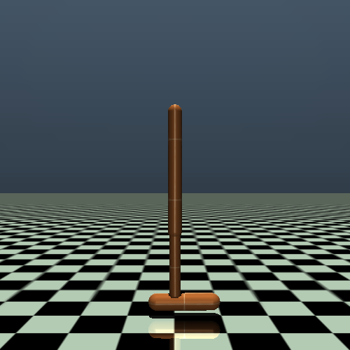
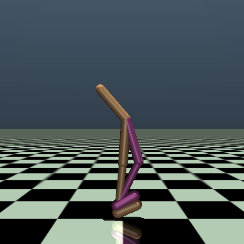
Figure 2: D4RL MuJoCo domains. From left to right, halfcheetah, hopper, walker2d.

MuJoCo datasets from D4RL are collected from three tasks of MuJoCo: Halfcheetah, Hopper and Walker2d, as illustrated in Figure 2. The quality of the datasets is categorized into the following types: random: samples from a randomly initialized policy. medium: 1M samples from an early-stopped SAC policy. medium-replay: 1M samples gathered from the replay buffer of a policy trained up to the performance of the medium agent. medium-expert: 50-50 split of medium-level data and expert-level data. expert: 1M samples from a logged expert policy.

The metric we use to evaluate the agent’s performance on MuJoCo datasets is the normalized score (NS). For a given MuJoCo dataset, NS is computed as:

$$NS=\frac{J_{\pi}-J_{random}}{J_{expert}-J_{random}}\times 100.$$

where $J_{\pi}$ is the performance of the policy under evaluation, $J_{random}$ is the performance of the random policy, and $J_{expert}$ is the performance of the expert policy.

C.2. Antmaze Datasets from D4RL

The Antmaze domain is a navigation task requiring an 8-DOF ”Ant” quadraped robot to reach a goal location. Due to the sparse reward setting of Antmaze, it is usually more challenging than MuJoCo domain. The Antmaze datasets contain three maze layouts: ”umaze”, ”medium” and ”large”, as shown in Figure 3. The datasets are collected in three flavors: (1) the robot is commanded to reach a specified goal from a fixed start point (antmaze-umaze-v0). (2) the robot is commanded to reach a random goal from a random start point (the ”diverse” datasets). (3) the robot is commanded to reach specific locations from a different set of specific start locations (the ”play” datasets). In our experiment, we use the six datasets to evaluate our method: antmaze-umaze-v0, antmaze-umaze-diverse-v0, antmaze-medium-diverse-v0, antmaze-medium-play-v0, antmaze-large-diverse-v0, antmaze-large-play-v0. When evaluating the performance of a policy on the Antmaze datasets, we use the success rate of reaching the goal as the metric.

Figure 3: D4RL Antmaze domains. From left to right, umaze, medium, large.

C.3. Implementation Details

We introduce the implementation of the baseline algorithms used in our work. For MOPO, we use the codebase re-implemented in Pytorch. For MOReL, we use the author-provided implementation. For MOBILE and RAMBO, we use the official implementation. For COMBO, we build the code based on MOPO. For the implementation of AMOReL and SUMO, we have included the code in the supplementary materials.

We then introduce the hyperparameter setup in our experiments. We present the main hyperparameter setup for AMOReL+SUMO and MOPO+SUMO in Table 6. For other baseline algorithms, we use the default hyperparameters suggested in original papers.

Table 6: Hyperparameter setup for AMOReL+SUMO and MOPO+SUMO.

Hyperparameter	Value
SUMO
$k$	1
Search vector	$s\oplus a\oplus s^{\prime}$
Distance measure	Euclidean distance
AMOReL
Model ensemble size	7
Model hidden layer	$(400,400,400,400)$
Actor and Critic hidden layer	$(256,256,256)$
Batch size	256
Optimizer	Adam (Kingma and Ba 2014)
Actor learning rate	$3\times 10^{-4}$
Critic learning rate	$3\times 10^{-4}$
$\alpha$	5
$\eta$	0.9
MOPO
Model ensemble size	7
Model hidden layer	$(400,400,400,400)$
Actor and Critic hidden layer	$(256,256,256)$
Batch size	256
Optimizer	Adam
Actor learning rate	$3\times 10^{-4}$
Critic learning rate	$3\times 10^{-4}$
$\lambda$	1
$\eta$	0.9

C.4. Compute Infrastructure

We list our hardware specifications as follows:

• GPU: NVIDIA RTX 3090 ($\times$8)

• CPU: AMD EPYC 7452

We also list our software specifications as follows:

• Python: 3.8.18

• Pytorch: 1.12.1+cu113

• Gym: 0.22.0

• MuJoCo: 2.0

• D4RL: 1.1

Table 7: Average training time comparison between base algorithms and their version with SUMO added on 15 MuJoCo datasets. The training steps are set to 1M.

	MOPO	AMOReL
Base	7h23m	8h46m
+SUMO	6h41m	8h03m

C.5. Time Cost

Given that SUMO involves KNN search which may be time consuming in large and high-dimensional datasets, it is essential to examine the time cost incurred by SUMO compared to model ensemble-based methods. We conduct experiments on all 15 MuJoCo datasets and compare the average training time cost of MOPO+SUMO and MOReL+SUMO against their base algorithms, with a total of 1M training steps. The results are shown in Table 7. The results indicate that SUMO does not bring more time cost than model ensemble-based methods, and even less, thanks to the efficient implementation of FAISS.

Appendix D D. More Experimental Results

D.1. Experimental Results on Antmaze Datasets

Table 8: Comparison of MOPO+SUMO and AMOReL+SUMO against MOPO and AMOReL on Antmaze ”-v0” domains. We run each algorithm for 1M gradient steps with 5 random seeds.

Task Name	MOPO		AMOReL
	SUMO	Base	SUMO	Base
Umaze	23.0	0.0	12.2	0.0
Umaze-Diverse	0.0	0.0	0.0	0.0
Medium-Play	13.4	0.0	0.0	0.0
Medium-Diverse	19.0	0.0	7.7	0.0
Large-Play	0.0	0.0	0.0	0.0
Large-Diverse	0.0	0.0	0.0	0.0
Average Score	9.2	0.0	3.3	0.0

Compared with MuJoCo datasets used and evaluated in the main text, Antmaze datasets from D4RL benchmark are much more challenging for model-based offline RL algorithms. To examine whether SUMO can also benefit base algorithms in Antmaze tasks, we conduct extensive experiments on top of MOPO and AMOReL on 6 Antmaze datasets: antmaze-umaze, antmaze-umaze-diverse, antmaze-medium-diverse, antmaze-medium-play, antmaze-large-diverse, antmaze-large-play, and compare the final performance between base algorithms and with SUMO added. The version of Antmaze datasets we use is v0.

The experimental results are presented in Table 8. It is clear that MOPO and AMOReL both struggle in all Antmaze tasks, achieving a score of zero. After integrating with SUMO, the performance of MOPO and AMOReL on some datasets has raised, indicating the agent learns a meaningful policy. This shows the efficacy of SUMO in challenging Antmaze domains.

D.2. More Comparison with Other Uncertainty Estimation Methods

In the main text, we show the superiority of SUMO over common model ensemble-based methods. In this part, we further compare SUMO with other uncertainty estimation methods for model-based offline RL from more recent literatures. We list our baselines as follows:

Count-based Estimation (CE). The method used by (Kim and Oh 2023), which utilizes the count estimates of state-action pairs to quantify the model uncertainty.

Riemannian Pullback Metric (RPM). The method used by (Tennenholtz and Mannor 2022). It estimates the sample uncertainty by computing its KNN distance to the data in the dataset using the Riemannian pullback metric.

We follow the experimental setup in Section Experiment of the main text, and compare SUMO with CE and RPM on D4RL datasets, using $\rho$ and $r$ as evaluating metrics. The comparison results are listed in Table 9. The results reveal that SUMO is comparable to CE and RPM in detecting OOD samples. However, using CE or RPM will bring heavy computational burden and cumbersome algorithmic procedures.

Table 9: Spearman rank ($\rho$) and Pearson bivariate ($r$) correlations comparison of SUMO with CE and RPM. We run each experiment by 5 different seeds and report the average $\rho$ and $r$.

Task Name	CE		RPM		SUMO
	$\mathbf{\rho}$	$r$	$\mathbf{\rho}$	$r$	$\mathbf{\rho}$	$r$
half-m	0.87	0.79	0.80	0.74	0.84	0.77
hopper-m	0.81	0.72	0.83	0.78	0.86	0.79
walker2d-m	0.86	0.77	0.79	0.76	0.82	0.71
half-m-e	0.85	0.74	0.76	0.70	0.88	0.81
hopper-m-e	0.77	0.63	0.70	0.65	0.75	0.68
walker2d-m-e	0.83	0.81	0.77	0.72	0.84	0.80
Mean	0.83	0.74	0.78	0.73	0.83	0.76

D.3. More Ablation Study Results

Table 10: Normalized average score comparison of MOPO+SUMO and AMOReL+SUMO w/ and w/o the reward dimension in the search vector. w/ $r$ means including the reward dimension, and w/o $r$ means excluding the reward dimension. Each experiment is run with 5 random seeds.

Task Name	MOPO+SUMO		AMOReL+SUMO
	w/ $r$	w/o $r$	w/ $r$	w/o $r$
half-r	37.1	37.2	43.9	44.2
hopper-r	24.9	24.5	32.2	32.4
walker2d-r	13.3	13.1	19.8	21.0
half-m-r	73.2	73.1	76.7	76.8
hopper-m-r	64.2	65.4	88.1	88.7
walker2d-m-r	68.9	70.3	67.8	65.3
half-m	66.2	68.9	84.2	82.1
hopper-m	76.7	74.6	94.3	95.0
walker2d-m	56.9	57.3	66.3	67.4
half-m-e	84.3	84.1	99.6	99.4
hopper-m-e	88.5	88.1	100.7	101.5
walker2d-m-e	82.2	81.9	113.4	112.3
half-e	87.8	87.1	110.2	112.3
hopper-e	101.9	101.2	106.5	105.4
walker2d-e	115.2	114.4	105.9	106.3
Average Score	69.4	69.4	80.6	80.7

In this part, we supplement the ablation study results over whether including the reward dimension into the search vector affects the performance of SUMO. We choose $(s\oplus a\oplus s^{\prime})$ as the base search vector and examine whether including the reward into the search vector, i.e., $(s\oplus a\oplus r\oplus s^{\prime})$ can incur a distinct performance for SUMO.

The base algorithms we choose are MOPO+SUMO and AMOReL+SUMO, we use $(s\oplus a\oplus s^{\prime})$ and $(s\oplus a\oplus r\oplus s^{\prime})$ as the search vector and conduct experiments on D4RL MuJoCo datasets. The results are shown in Table 10. We can see almost no difference on algorithm performance between these two search vectors, indicating that whether including the reward dimension for KNN search has alomost no effect on the efficacy of SUMO. Therefore, we can simply drop the reward dimension for KNN search.

D.4. More Parameter Study Results

In the main text, we conduct the parameter study for $k$ value of SUMO. In this part, we provide more parameter study results for AMOReL+SUMO and MOPO+SUMO.

For AMOReL+SUMO, we focus on the threshold coefficient $\alpha$. For MOPO+SUMO, we focus on the penalty coefficient $\lambda$ and the sampling coefficient $\eta$. We conduct experiments on MuJoCo datasets from D4RL.

For AMOReL+SUMO:

• Sampling coefficient $\eta$: $\eta$ determines the proportion of dataset samples used for training. A larger $\eta$ means more real samples for training, while a smaller $\eta$ means more synthetic samples for training. We vary the value of $\eta$ to $\{0.05,0.5,0.9\}$, and conduct experiments on halfcheetah-medium-expert-v2. The results are shown in Figure 4 Left. We find that a better performance is achieved when using more real samples for training, for example, $\eta=0.9$. Therefore, in this work, we set $\eta$ to 0.9.

• Threshold coefficient $\alpha$: $\alpha$ controls the size of the trajectory truncation threshold. A larger $\alpha$ results in a larger threshold, allowing more synthetic samples to be used for training. A smaller $\alpha$ leads to a smaller threshold, allowing fewer synthetic samples for training. We use halfcheetah-medium-expert for experiments, with different $\alpha\in\{1,5,10\}$. The results are shown in Figure 4 Right. We find that both too large and too small values for $\alpha$ do not perform well. An appropriate value for $\alpha$, such as $\alpha=5$, leads to better performance.

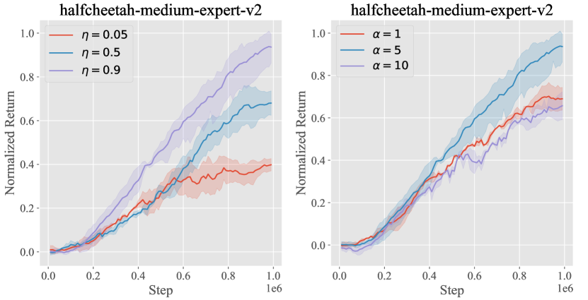
Figure 4: Parameter study on $\alpha$ of AMOReL+SUMO. We run each experiment with 5 random seeds. The shaded region denotes the standard deviation.

Figure 5: Left: Parameter study on $\eta$ of MOPO+SUMO. Right: Parameter study on $\lambda$ of MOPO+SUMO. We run each experiment with 5 random seeds and the shaded region captures the standard deviation.

For MOPO+SUMO:

• Sampling coefficient $\eta$: Similar to AMOREL+SUMO, $\eta$ controls the proportion of real samples for training. We conduct experiments on halfcheetah-medium-expert-v2, with different $\eta\in\{0.05,0.5,0.9\}$, and present the experimental results in Figure 5 Left. We find that using larger $\eta$ leads to a better performance.

• Penalty coefficient $\lambda$: $\lambda$ determines the degree of reward penalty. A larger $\lambda$ means a greater penalty for synthetic samples. We vary $\lambda$ to $\{1,5,10\}$, and conduct experiments on halfcheetah-medium-expert-v2. The results are shown in Figure 5 Right. We find that MOPO-SUMO is robust to the value of $\lambda$. Therefore, in this work, we set $\lambda=1$.

D.5. Full Comparison with More Baselines

In the main text, we have compared the performance of base algorithms with and without applying SUMO for uncertainty estimation. These base algorithms (MOPO, AMOReL, MOReL and MOBILE) all need to estimate and utilize uncertainty. In this part, we add more baselines which discard uncertainty estimation for comparison. We choose COMBO and RAMBO as baselines and conduct experiments on 15 D4RL MuJoCo datasets. The full experimental results are listed in Table 11. We can see SUMO can bring performance bonus to base algorithms, surpassing the compared baselines. Especially, the average score of AMOReL is lower than that of COMBO and RAMBO, but AMOReL+SUMO shows a superior performance to COMBO and RAMBO.

Table 11: Normalized average score comparison of different base algorithms with and without SUMO, as well as other model-based offline algorithms including COMBO and RAMBO on 15 D4RL MuJoCo datasets, and the version of datasets we use is ”-v2”. We abbreviate ”halfcheetah” as ”half”, ”random” as ”r”, ”medium” as ”m”, ”medium-replay” as ”m-r”, ”medium-expert” as ”m-e” and ”expert” as ”e”. We run each algorithm for 1M gradient steps with 5 random seeds. We report the final average performance and $\pm$ captures the standard deviation. Bold numbers with a green background represent the best average scores within each group.

Task Name	MOPO		AMOReL		MOReL		MOBILE		COMBO	RAMBO
	SUMO	Base	SUMO	Base	SUMO	Base	SUMO	Base
half-r	37.2$\pm$1.9	34.9$\pm$1.4	44.2$\pm$2.1	31.8$\pm$2.4	37.3$\pm$2.1	29.8$\pm$1.2	34.9$\pm$2.1	37.8$\pm$2.9	34.3$\pm$1.9	39.7$\pm$1.9
hopper-r	24.5$\pm$0.9	19.4$\pm$0.7	29.7$\pm$0.6	32.4$\pm 1.2$	33.2$\pm$0.7	30.1$\pm$1.0	30.8$\pm$0.9	32.6 $\pm$ 1.2	25.6$\pm$0.8	21.6$\pm$6.9
walker2d-r	11.4$\pm$1.3	13.1$\pm$1.1	20.3$\pm$0.2	21.0$\pm$0.3	17.8$\pm$0.6	19.4$\pm$0.3	27.9$\pm$2.0	16.3$\pm$ 4.6	11.3$\pm$0.8	13.4$\pm$5.4
half-m-r	73.1$\pm$2.1	65.0$\pm$3.3	76.8$\pm$2.7	49.6$\pm$2.3	67.9$\pm$2.5	51.2$\pm$1.9	76.2$\pm$1.3	67.9$\pm$2.0	51.0$\pm$2.3	67.1$\pm$1.2
hopper-m-r	65.4$\pm$3.2	38.8$\pm$2.4	88.7$\pm$1.3	80.5$\pm$1.0	83.9$\pm$1.3	76.3$\pm$1.0	109.9$\pm$1.4	104.9$\pm$0.9	82.2$\pm$2.1	92.6$\pm$4.5
walker2d-m-r	70.3$\pm$0.6	74.8$\pm$1.5	65.3$\pm$2.7	46.0$\pm$1.9	61.3$\pm$3.1	48.1$\pm$4.2	78.2$\pm$1.5	83.9$\pm$1.3	83.8$\pm$1.1	83.4$\pm$9.7
half-m	68.9$\pm$2.3	73.1$\pm$2.7	82.1$\pm$2.8	69.2$\pm$1.2	57.9$\pm$1.2	62.4$\pm$1.3	84.3$\pm$2.4	75.1$\pm$1.5	59.5$\pm$0.9	75.1$\pm$0.8
hopper-m	74.6$\pm$1.9	45.6$\pm$2.5	95.0$\pm$2.1	87.2$\pm$3.4	82.1$\pm$1.4	84.7$\pm$3.1	104.8$\pm$2.1	102.9$\pm$1.9	83.6$\pm$2.4	92.4$\pm$6.7
walker2d-m	57.3$\pm$1.6	42.3$\pm$0.8	67.4$\pm$0.9	71.2$\pm$1.3	77.1$\pm$3.5	67.6$\pm$2.2	94.1$\pm$2.5	89.1$\pm$1.0	89.8$\pm$1.8	87.7$\pm$2.1
half-m-e	84.1$\pm$1.4	76.6$\pm$1.0	99.4$\pm$3.6	90.6$\pm$2.1	98.6$\pm$3.5	92.3$\pm$4.6	106.6$\pm$2.4	109.2$\pm$3.8	84.0$\pm$1.2	92.1$\pm$3.5
hopper-m-e	88.1$\pm$1.9	69.1$\pm$1.2	101.5$\pm$0.4	106.2$\pm$1.5	105.8$\pm$1.4	102.4$\pm$0.9	107.8$\pm$0.7	110.1$\pm$1.3	104.6$\pm$3.4	83.1$\pm$7.8
walker2d-m-e	81.9$\pm$1.6	75.4$\pm$1.1	109.6$\pm$0.7	92.3$\pm$0.9	86.1$\pm$1.8	90.4$\pm$1.4	122.8$\pm$0.4	115.9$\pm$0.8	98.1$\pm$0.4	62.1$\pm$13.4
half-e	87.1$\pm$1.2	88.7$\pm$1.6	112.3$\pm$2.5	103.2$\pm$1.9	109.9$\pm$2.1	105.8$\pm$1.6	111.5$\pm$1.5	113.1$\pm$2.1	100.4$\pm$0.2	107.5 $\pm$ 11.6
hopper-e	101.2$\pm$ 1.8	83.9$\pm$0.7	105.4$\pm$0.6	94.5$\pm$0.3	101.8$\pm$1.9	92.5$\pm$1.0	115.9 $\pm$ 2.9	112.4$\pm$3.5	111.4$\pm$1.5	114.2$\pm$17.9
walker2d-e	114.4$\pm$1.1	95.3$\pm$3.4	106.3$\pm$1.3	107.2$\pm$1.0	106.2$\pm$1.5	108.3$\pm$2.1	116.3$\pm$1.5	113.7$\pm$1.1	108.2$\pm$2.0	102.3$\pm$3.1
Average score	69.3	59.7	80.3	72.2	75.1	70.7	88.2	85.6	73.7	75.6

References

- An et al. (2021) An, G.; Moon, S.; Kim, J.-H.; and Song, H. O. 2021. Uncertainty-based offline reinforcement learning with diversified q-ensemble. Advances in Neural Information Processing Systems, 34: 7436–7447.
- Csiszár and Körner (2011) Csiszár, I.; and Körner, J. 2011. Information theory: coding theorems for discrete memoryless systems. Cambridge University Press.
- Fu et al. (2020) Fu, J.; Kumar, A.; Nachum, O.; Tucker, G.; and Levine, S. 2020. D4rl: Datasets for deep data-driven reinforcement learning. arXiv preprint arXiv:2004.07219.
- Fujimoto and Gu (2021) Fujimoto, S.; and Gu, S. S. 2021. A minimalist approach to offline reinforcement learning.
- Fujimoto, Meger, and Precup (2019) Fujimoto, S.; Meger, D.; and Precup, D. 2019. Off-policy deep reinforcement learning without exploration. In International Conference on Machine Learning, 2052–2062. PMLR.
- Garcia and Rachelson (2013) Garcia, F.; and Rachelson, E. 2013. Markov decision processes. Markov Decision Processes in Artificial Intelligence, 1–38.
- Haarnoja et al. (2018) Haarnoja, T.; Zhou, A.; Abbeel, P.; and Levine, S. 2018. Soft actor-critic: Off-policy maximum entropy deep reinforcement learning with a stochastic actor. In International conference on machine learning, 1861–1870. PMLR.
- Johnson, Douze, and Jégou (2019) Johnson, J.; Douze, M.; and Jégou, H. 2019. Billion-scale similarity search with gpus. IEEE Transactions on Big Data, 7(3): 535–547.
- Kidambi et al. (2020) Kidambi, R.; Rajeswaran, A.; Netrapalli, P.; and Joachims, T. 2020. Morel: Model-based offline reinforcement learning. Advances in Neural Information Processing Systems, 33: 21810–21823.
- Kim and Oh (2023) Kim, B.; and Oh, M.-h. 2023. Model-based offline reinforcement learning with count-based conservatism. In International Conference on Machine Learning, 16728–16746. PMLR.
- Kingma and Ba (2014) Kingma, D. P.; and Ba, J. 2014. Adam: A method for stochastic optimization. arXiv preprint arXiv:1412.6980.
- Kumar et al. (2019) Kumar, A.; Fu, J.; Soh, M.; Tucker, G.; and Levine, S. 2019. Stabilizing off-policy q-learning via bootstrapping error reduction. Advances in Neural Information Processing Systems, 32.
- Kumar et al. (2020) Kumar, A.; Zhou, A.; Tucker, G.; and Levine, S. 2020. Conservative q-learning for offline reinforcement learning. Advances in Neural Information Processing Systems, 33: 1179–1191.
- Levine et al. (2020) Levine, S.; Kumar, A.; Tucker, G.; and Fu, J. 2020. Offline reinforcement learning: Tutorial, review, and perspectives on open problems. arXiv preprint arXiv:2005.01643.
- Liu et al. (2023) Liu, X.-Y.; Zhou, X.-H.; Xie, X.-L.; Liu, S.-Q.; Feng, Z.-Q.; Li, H.; Gui, M.-J.; Xiang, T.-Y.; Huang, D.-X.; and Hou, Z.-G. 2023. DOMAIN: MilDly COnservative Model-BAsed OfflINe Reinforcement Learning. arXiv preprint arXiv:2309.08925.
- Lockwood and Si (2022) Lockwood, O.; and Si, M. 2022. A review of uncertainty for deep reinforcement learning. In Proceedings of the AAAI Conference on Artificial Intelligence and Interactive Digital Entertainment.
- Lu et al. (2021) Lu, C.; Ball, P. J.; Parker-Holder, J.; Osborne, M. A.; and Roberts, S. J. 2021. Revisiting Design Choices in Offline Model-Based Reinforcement Learning. arXiv preprint arXiv:2110.04135.
- Lyu, Li, and Lu (2022) Lyu, J.; Li, X.; and Lu, Z. 2022. Double Check Your State Before Trusting It: Confidence-Aware Bidirectional Offline Model-Based Imagination. In Neural Information Processing Systems.
- Lyu et al. (2022) Lyu, J.; Ma, X.; Li, X.; and Lu, Z. 2022. Mildly conservative Q-learning for offline reinforcement learning. Advances in Neural Information Processing Systems, 35: 1711–1724.
- Lyu et al. (2024) Lyu, J.; Ma, X.; Wan, L.; Liu, R.; Li, X.; ; and Lu, Z. 2024. SEABO: A Simple Search-Based Method for Offline Imitation Learning. In International Conference on Learning Representations.
- Pan et al. (2020) Pan, F.; He, J.; Tu, D.; and He, Q. 2020. Trust the model when it is confident: Masked model-based actor-critic. Advances in Neural Information Processing Systems, 33: 10537–10546.
- Prudencio, Maximo, and Colombini (2023) Prudencio, R. F.; Maximo, M. R.; and Colombini, E. L. 2023. A survey on offline reinforcement learning: Taxonomy, review, and open problems. IEEE Transactions on Neural Networks and Learning Systems.
- Ran et al. (2023) Ran, Y.; Li, Y.-C.; Zhang, F.; Zhang, Z.; and Yu, Y. 2023. Policy Regularization with Dataset Constraint for Offline Reinforcement Learning. arXiv preprint arXiv:2306.06569.
- Rigter, Lacerda, and Hawes (2022) Rigter, M.; Lacerda, B.; and Hawes, N. 2022. Rambo-rl: Robust adversarial model-based offline reinforcement learning. Advances in neural information processing systems, 35: 16082–16097.
- Singh et al. (2003) Singh, H.; Misra, N.; Hnizdo, V.; Fedorowicz, A.; and Demchuk, E. 2003. Nearest neighbor estimates of entropy. American journal of mathematical and management sciences, 23(3-4): 301–321.
- Sun et al. (2023) Sun, Y.; Zhang, J.; Jia, C.; Lin, H.; Ye, J.; and Yu, Y. 2023. Model-Bellman inconsistency for model-based offline reinforcement learning. In International Conference on Machine Learning.
- Sutton and Barto (2018) Sutton, R. S.; and Barto, A. G. 2018. Reinforcement learning: An introduction. MIT press.
- Tennenholtz and Mannor (2022) Tennenholtz, G.; and Mannor, S. 2022. Uncertainty estimation using riemannian model dynamics for offline reinforcement learning. Advances in Neural Information Processing Systems, 35: 19008–19021.
- Van Amersfoort et al. (2021) Van Amersfoort, J.; Smith, L.; Jesson, A.; Key, O.; and Gal, Y. 2021. On feature collapse and deep kernel learning for single forward pass uncertainty. arXiv preprint arXiv:2102.11409.
- Wang et al. (2021) Wang, J.; Li, W.; Jiang, H.; Zhu, G.; Li, S.; and Zhang, C. 2021. Offline reinforcement learning with reverse model-based imagination. Advances in Neural Information Processing Systems, 34: 29420–29432.
- Yang et al. (2024) Yang, K.; Tao, J.; Lyu, J.; and Li, X. 2024. Exploration and Anti-Exploration with Distributional Random Network Distillation. ArXiv, abs/2401.09750.
- Yu et al. (2021) Yu, T.; Kumar, A.; Rafailov, R.; Rajeswaran, A.; Levine, S.; and Finn, C. 2021. Combo: Conservative offline model-based policy optimization. Neural Information Processing Systems, 34: 28954–28967.
- Yu et al. (2020) Yu, T.; Thomas, G.; Yu, L.; Ermon, S.; Zou, J. Y.; Levine, S.; Finn, C.; and Ma, T. 2020. Mopo: Model-based offline policy optimization. Advances in Neural Information Processing Systems, 33: 14129–14142.
- Zhang et al. (2023a) Zhang, H.; Shao, J.; He, S.; Jiang, Y.; and Ji, X. 2023a. DARL: distance-aware uncertainty estimation for offline reinforcement learning. In Proceedings of the AAAI Conference on Artificial Intelligence.
- Zhang et al. (2023b) Zhang, J.; Lyu, J.; Ma, X.; Yan, J.; Yang, J.; Wan, L.; and Li, X. 2023b. Uncertainty-Driven Trajectory Truncation for Data Augmentation in Offline Reinforcement Learning. In ECAI 2023, 3018–3025. IOS Press.