TIT/HEP-703

August, 2024

Integrals of motion in conformal field theory with $W$-symmetry and the ODE/IM correspondence
Katsushi Ito, Mingshuo Zhu
Department of Physics,
Tokyo Institute of Technology
Tokyo, 152-8551, Japan

We study the ODE/IM correspondence between two-dimensional $WA_{r}$/$WD_{r}$-type conformal field theories and the higher-order ordinary differential equations (ODEs) obtained from the affine Toda field theories associated with $A_{r}^{(1)}/D_{r}^{(1)}$-type affine Lie algebras. We calculate the period integrals of the WKB solution to the ODE along the Pochhammer contour, where the WKB expansions correspond to the classical conserved currents of the Drinfeld-Sokolov integrable hierarchies. We also compute the integrals of motion for $WA_{r}$($WD_{r}$) algebras on a cylinder. Their eigenvalues on the vacuum state are confirmed to agree with the period integrals up to the sixth order. These results generalize the ODE/IM correspondence to higher-order ODEs and can be used to predict higher-order integrals of motion.

1 Introduction

In two-dimensional conformal field theory (CFT), Integrals of motion (IoMs) play an important role in understanding the dynamics and symmetries of the system[1]. There is an infinite number of IoMs due to integrability; hence, their construction is a fundamental problem in CFT. In the minimal model of CFT [2], an explicit form of the IoMs and their eigenvalues in the vacuum state is obtained in terms of the energy-momentum (EM) tensor up to spin eight [1, 3]. So far, it has been generalized to the $WA_{2}$ model[4], a CFT with a spin 3 field, in [5, 6]. However, explicit construction of IoMs in higher spin $W\mathfrak{g}$ algebra is still an open question. We also note that IoMs play a crucial role in studying thermal correlators in CFT [7, 8, 9].

The IoMs in CFT with $W$-symmetry are defined as mutually commuting conserved quantities constructed from the energy-momentum tensor and $W$ currents[5]. On the complex plane, their commutation relations are obtained from the operator product expansions (OPEs) among the currents[10, 11, 12]. The computation of the OPE with the $W$-currents can be simplified by the free-field realization [4, 13]. Another interesting approach to finding the IoMs in CFT is to use the ODE/IM correspondence, which is the main subject of this paper.

The ODE/IM correspondence [14, 15] describes the relation between the spectral analysis of ordinary differential equations (ODEs) and the functional approach of two-dimensional quantum integrable models (IMs). For the Schrödinger type second-order ODE, the correspondence shows that the connection coefficients between the asymptotic solutions of the ODE around the singularities define the $Q$-, $T$-, and $Y$- functions of the quantum integrable model, or more precisely, the CFT. For example, the Q-function, which connects the basis of the solutions around the origin and infinity, satisfy the non-linear integral equations [16]. The zeros of the Q-functions determine the roots of the Bethe ansatz equations. The Y-functions that satisfy the thermodynamic Bethe ansatz (TBA) equations in the integrable theories correspond to the Borel resummation of the WKB period of the solutions of the ODE [17]. Both the integral equations provide the effective central charge of the CFT, which is characterized by the lowest conformal dimension of the primary field.

The IoMs and their eigenvalues on the vacuum state provide much information about CFT with extended symmetry. The local IoMs are obtained by the T-functions expanded in the power of the spectral parameter. For the Schrödinger equation with monomial potential, the IoMs of the minimal models [1] are shown to coincide with higher-order corrections to the specific WKB period for the ODE (see also [17]). A generalization to ${\cal N}=1$ supersymmetric minimal models has been studied in [18].

It is interesting to study a correspondence between the higher-order IoM and the WKB period for higher-order ODE. The ODE/IM correspondence for higher-order ODEs has been studied in [19, 20, 21, 22, 23, 24, 25, 26] based on integral equations, which provide a relation to CFT with $W$ currents. In particular, the $W\mathfrak{g}$ CFT corresponds to the linear differential system associated with the $\hat{\mathfrak{g}}^{\vee}$ affine Toda field equations modified by some conformal transformation. Such conformal transformation is necessary to produce the appropriate correction to the potential term in the ODE. So far, the correspondence between the IoMs in CFT with $W$ symmetry and the WKB periods has been observed for the $WA_{2}$ algebra [15, 9].

In the previous paper[27], we studied the WKB expansion of the solutions to the linear differential equations associated with classical affine Lie algebras. The linear differential equation can be diagonalized by the gauge transformation, which reduces to a set of first-order linear differential equations. The diagonalized connection in the fundamental representation is a generating function of the conserved currents of the integrable hierarchy in the Drinfeld-Sokolov reduction[28]. Moreover, the diagonalized connection satisfies the Riccati equation of the adjoint ODE, which is also satisfied by the top component of the solution to the adjoint linear problem. The WKB periods can be regarded as the conserved charges of the classical integrable hierarchy, which implies that the ODE/IM correspondence shows a nontrivial relation between classical and quantum theories.

The purpose of this paper is to find the IoMs in CFT with the $WA_{r}$ or $WD_{r}$ symmetry and explore the correspondence between them and the WKB integrals of the classical conserved charges of the $A_{r}^{(1)}$ and $D_{r}^{(1)}$ adjoint linear systems. These two adjoint linear systems are the same as their own ones, whose WKB solution is equivalent to the one for the higher-order ODE satisfied by the top component of the solution of the linear problem.

This paper is organized as follows. In section 2, we first carry out the WKB analysis on the $A_{r}^{(1)}$- and $D_{r}^{(1)}$-type higher-order ODEs given in [29, 24, 27]. Both can be obtained from the linear system of the modified affine Toda field equations. We then compute their WKB integrals along the Pochhammer contour up to the 8th order for general rank $r$. In section 3, we first define the CFT on a complex plane and present the EM tensor, $W$ currents, and their OPEs. Then, we introduce the free-field realization in $WA_{r}$ and $WD_{r}$ algebras and calculate the IoMs on the complex plane up to order six for some lower ranks. Finally, we define the IoMs on a cylinder and compute their eigenvalues on the vacuum state. In section 4, we compare the WKB integrals and the eigenvalue of the IoMs and confirm the ODE/IM correspondence for the linear problem associated with the $A_{r}^{(1)}$ and $D_{r}^{(1)}$ -types affine Lie algebras.

2 Modified affine Toda field equations and the linear system

In this section, we first define the linear problem for affine Toda field theories modified by a conformal transformation based on [30, 31, 24, 32, 33, 35]. We introduce the higher-order ODE satisfied by the top component of the solution to the linear problem and their WKB solutions. The WKB solutions correspond to the classical conserved currents of the Drinfeld-Sokolov reduction of the soliton hierarchy based on affine Lie algebras [28]. We then compute the integrals of the WKB solutions along the Pochhammer contour. These classical quantities will be compared with the conserved charges of the quantum IoMs in the CFT with $W$ symmetry, which are computed in the next section.

2.1 The WKB analysis of linear problem

We now introduce the affine Toda field theories in $2d$ Euclidean space with local holomorphic coordinates $z$ and $\bar{z}$. The action for affine Toda theory with rank-$r$ affine Lie algebra $\hat{\mathfrak{g}}$ is defined by

$$S[\phi]=\int\mathrm{d}^{2}z\left[\frac{1}{2}\partial_{z}\phi\cdot\partial_{\bar{z}}\phi+\left(\frac{m^{2}}{\beta}\right)\left(\sum_{i=1}^{r}\exp\left(\beta\alpha_{i}\cdot\phi\right)+\exp\left(\beta\alpha_{0}\cdot\phi\right)\right)\right],$$ (2.1)

where $\phi(z)=\left(\phi_{1}(z),\ldots,\phi_{r}(z)\right)$ is a vector of $r$ free bosons, $m$ is the mass parameter and $\beta$ is the coupling constant. $\alpha_{i}(\alpha_{0})$ $(i=1,\dots,r)$ are the simple(affine) roots normalized whose squared length is two. We denote the coroots of $\alpha_{i}$ by $\alpha^{\vee}_{i}=2\alpha_{i}/|\alpha_{i}|^{2}$. If one removes the potential term including $\alpha_{0}$, the action will reduce to the one of non-affine Toda field theory. The equation of motion for the action (2.1) is given by

$$\partial_{\bar{z}}\partial_{z}\phi(z,\bar{z})-\Big{(}\frac{m^{2}}{\beta}\Big{)}\left[\sum_{i=1}^{r}\alpha_{i}\exp\big(\beta\alpha_{i}\cdot\phi\big{missing})+\alpha_{0}\exp\big(\beta\alpha_{0}\cdot\phi\big{missing})\right]=0.$$ (2.2)

Under the conformal transformation:

$$z\rightarrow w(z),\quad\bar{z}\rightarrow\bar{w}(\bar{z}),\quad\phi(z,\bar{z})\rightarrow\hat{\phi}(z,\bar{z})=\phi(w,\bar{w})+\frac{\rho^{\vee}}{\beta}\log(\partial_{z}w\partial_{\bar{z}}\bar{w}),$$ (2.3)

the equation (2.2) written in terms of $(w,\bar{w})$ coordinates becomes

$$\partial_{\bar{z}}\partial_{z}\phi(z,\bar{z})-\left(\frac{m^{2}}{\beta}\right)\left[\sum_{i=1}^{r}\alpha_{i}\exp\big(\beta\alpha_{i}\cdot\phi\big{missing})+p(z)\bar{p}(\bar{z})\alpha_{0}\exp\big(\beta\alpha_{0}\cdot\phi\big{missing})\right]=0$$ (2.4)

with

$$p(z)=(\partial_{z}w)^{h},\quad\bar{p}(\bar{z})=(\partial_{\bar{z}}\bar{w})^{h}.$$ (2.5)

In Eq.(2.3), the Weyl(co-Weyl) vectors $\rho(\rho^{\vee})$ is the sum of the fundamental(co-fundamental) weights

$$\rho=\sum_{i=1}^{r}\omega_{i},\quad\rho^{\vee}=\sum_{i=1}^{r}\omega^{\vee}_{i},$$ (2.6)

and the fundamental(co-fundamental) weights $\omega_{i}(\omega_{i}^{\vee})$ are the vectors dual to roots(coroots) $\alpha_{i}(\alpha_{i}^{\vee})$

$$\omega_{i}\cdot\alpha_{j}^{\vee}=\omega_{i}^{\vee}\cdot\alpha_{j}=\delta_{ij},\quad(1\leq i\leq r)$$ (2.7)

Finally, the Coxeter number $h$ is given by $h=r+1$ for $A_{r}$, and $2r-2$ for $D_{r}$ in Eq.(2.5). There is an important relation between the Weyl vector $\rho$ and the dual Coxter number $h^{\vee}$ that is equal to $h$ for a simply-laced Lie algebra $\mathfrak{g}$:

$$\rho^{2}=\frac{h^{\vee}\;\text{dim}(\mathfrak{g})}{12}.$$ (2.8)

The modified affine Toda field equation (2.4) can be rewritten as the integrability condition for a pair of linear systems

$${\cal L}\Psi=\bar{\cal L}\Psi=0,$$ (2.9)

where ${\cal L}$ and $\bar{\cal L}$ denote the Lax operators

$$\begin{split}&\mathcal{L}=\partial_{z}+\sum_{i=1}^{r}\beta\partial_{z}\phi_{i}(z)H_{i}+\lambda\left(\sum_{i=1}^{r}E_{\alpha_{i}}+p(z)E_{\alpha_{0}}\right),\\ &\bar{\mathcal{L}}=\partial_{\bar{z}}+\lambda^{-1}e^{-\beta\sum_{i=1}^{r}\phi_{i}H_{i}}\left(\sum_{i=1}^{r}E_{-\alpha_{i}}+\bar{p}(\bar{z})E_{-\alpha_{0}}\right)e^{\beta\sum_{i=1}^{r}\phi_{i}H_{i}}.\end{split}$$ (2.10)

Here $E_{\pm\alpha_{0}}$, $E_{\pm\alpha_{i}}$ and $H_{i}=\alpha^{\vee}_{i}\cdot H$ ($i=1,\dots,r$) are the Chevalley generators of affine Lie algebra $\hat{\mathfrak{g}}$, and $\lambda$ is the spectral parameter.

We will take the light-cone limit and the conformal limit of the linear system (2.9). First, we set

$$p(z)=z^{hM}-s^{hM},$$ (2.11)

where $h$ is the Coxeter number, $M$ is a positive real number with $M>(1/h-1)$ and $s$ is an arbitrary parameter. The function $p(z)$ determines the behaviour of $\phi(z)$ at infinity [30, 24], while at the origin, we impose the boundary condition for $\phi(z)$ as [30]

$$\phi(z)=\frac{l}{\beta}\log(z)+\mathcal{O}(1),$$ (2.12)

with $l$ an $r$-dimensional vector. We first take the light-cone limit $\bar{z}\rightarrow 0$ and the conformal limit $\lambda\rightarrow\infty$

$$z=\lambda^{-\frac{1}{1+M}}x,\quad s^{hM}=\lambda^{-\frac{hM}{1+M}}E$$ (2.13)

with $x$ and $E$ finite. In these limits, the linear problem reduces to a single holomorphic linear differential equation. Further rescaling $x$ and $E$ as

$$x\rightarrow\epsilon^{\frac{1}{1+M}}x,\quad E\rightarrow\epsilon^{\frac{hM}{1+M}},$$ (2.14)

and making the gauge transformation as [26], the holomorphic linear problem (2.9) becomes the first-order linear differential equation

$$\begin{split}&\epsilon\partial_{x}\Psi+\epsilon\frac{1}{x}(l\cdot H)\Psi+\left(\sum_{i=1}^{r}E_{\alpha_{i}}+p(x)E_{\alpha_{0}}\right)\Psi=0\\ \end{split}$$ (2.15)

with $p(x)=x^{hM}-1$. We will consider the WKB solution of the linear problem (2.15) for $\hat{\mathfrak{g}}=A_{r}^{(1)}$ and $D_{r}^{(1)}$.

The WKB analysis of the $A_{r}^{(1)}$ type

Now we focus on the linear problem (2.15) in the $(r+1)$-dimensional fundamental representation of $A_{r}$. Let $\left\{\epsilon_{1},\ldots,\epsilon_{r+1}\right\}$ be the weights of this representation. They satisfy the conditions:

$$\begin{split}&\epsilon_{i}\cdot\epsilon_{j}=\delta_{ij}-\frac{1}{r+1},\quad\sum_{i=1}^{r+1}\epsilon_{i}=0,\\ &\sum_{i<j}\epsilon_{i}\otimes\epsilon_{j}=-\frac{1}{2}\mathbb{1},\quad\sum_{i=1}^{r+1}i\epsilon_{i}=-\rho^{\vee}.\end{split}$$ (2.16)

The simple roots of $A_{r}$ are given by $\alpha_{i}=\epsilon_{i}-\epsilon_{i+1}$ $(i=1,\dots,r$). The linear equation for $\Psi$ (2.15) in the representation reduces to the $(r+1)$-th order ODE for the first component $\psi$ of $\Psi$ [23, 27].

$$\left[\epsilon^{r+1}\left(\partial_{x}-\frac{l_{1}}{x}\right)\left(\partial_{x}-\frac{l_{2}}{x}\right)\dots\left(\partial_{x}-\frac{l_{r}}{x}\right)\left(\partial_{x}-\frac{l_{r+1}}{x}\right)+(-1)^{r}p(x)\right]\psi(x,\epsilon)=0$$ (2.17)

with $l_{i}=\epsilon_{i}\cdot l$ and $h=r+1$ for $A_{r}^{(1)}$. This ODE is the same as that appears in the ODE/IM correspondence [14, 22]. To find the WKB solution, it is convenient to expand the first term in (2.17) and rewrite it in the form

$$\left[(\epsilon\partial_{x})^{h}+\sum_{i=2}^{h}\epsilon^{i}\frac{L_{i}}{x^{i}}(\epsilon\partial_{x})^{h-i}+(-1)^{r}p(x)\right]\psi(x,\epsilon)=0$$ (2.18)

with the coefficients $L_{i}$ some functions of $l$. In particular, they are expressed in terms of the the elementary symmetric polynomials of $(\epsilon_{i},l+\rho)$:

$$s_{k}=\sum_{1\leq i_{1}<i_{2}<\dots<i_{k}\leq r+1}(\epsilon_{i_{1}},l+\rho)(\epsilon_{i_{2}},l+\rho)\dots(\epsilon_{i_{k}},l+\rho).$$

The first five coefficients are found to be

$$\begin{split}L_{2}&=s_{2}+\frac{1}{24}r(r+1)(r+2),\\ L_{3}&=-s_{3}-(r-1)L_{2},\\ L_{4}&=s_{4}+\frac{3}{2}(r-2)s_{3}+\frac{1}{24}(r+24)(r-1)(r-2)s_{2}\\ &+\frac{1}{5760}(5r+228)(r+2)(r+1)r(r-1)(r-2),\\ L_{5}&=-s_{5}-2(r-3)s_{4}-\frac{1}{24}(r-3)(r-2)(r+44)s_{3}\\ &-\frac{1}{12}(r-3)(r-2)(r-1)(r+12)s_{2}\\ &-\frac{1}{2880}(r-3)(r-2)(r-1)r(r+1)(r+2)(5r+108),\end{split}$$ (2.19)

and the 6th, 7th, and 8th orders are listed in Appendix A.

We now study the WKB solution of (2.18). Let us consider the WKB expansion of $\psi(x,\epsilon)$, where $\epsilon$ is an expansion parameter:

$$\psi(x,\epsilon) =\exp(\frac{1}{\epsilon}\int^{x}dx\,S(x,\epsilon)),$$ (2.20)

$$S(x,\epsilon) =\sum_{i=0}^{\infty}\epsilon^{i}S_{i}(x).$$ (2.21)

Substituting Eq.(2.20) into Eq.(2.18), one obtains the Riccati equation for $S(x,\epsilon)$:

$$(\epsilon\partial_{x}+S)^{r}S+\sum_{i=2}^{r+1}\frac{L_{i}}{x^{i}}(\epsilon\partial_{x}+S)^{r-i}S+(-1)^{r}p(x)=0,$$ (2.22)

where we define $(\epsilon\partial_{x}+S)^{-1}S=1$ in the summation. Then we expand $S(x,\epsilon)$ as Eq.(2.21) and solve the equation (2.22) recursively. Here the first two terms of order $\epsilon^{n}$ $(n=0,1)$ are

$$\begin{split}\epsilon^{0}:\;\;(-1)^{r}p(x)+S_{0}^{r+1}=0,\quad\epsilon^{1}:\;\;\frac{1}{2}(r+1)S_{0}^{r-1}\left(rS_{0}^{\prime}+2S_{0}S_{1}\right)=0.\end{split}$$ (2.23)

The higher-order terms can be determined similarly. Their solutions are given by

$$\begin{split}S_{0}(x)&=-p(x)^{\frac{1}{h}},\\ S_{1}(x)&=\frac{h-1}{2h}\partial_{x}\log(p),\\ S_{2}(x)&=\frac{L_{2}}{h}p^{-\frac{1}{h}}x^{-2}-\frac{(h-1)(h+1)M(hM-1)}{12}p^{-\frac{1}{h}-1}x^{hM-2}\\ \;\;\;\;\;\;\;&+\frac{(h-1)(h+1)(2h+1)M^{2}}{24}p^{-\frac{1}{h}-2}x^{2hM-2},\\ \dots{}\end{split}$$ (2.24)

Note that $S_{0}(x)$ has $(r+1)$ solutions with phases given by $(r+1)$-th root of unity. Following the convention in [27], we choose the $-$ sign. It has been shown that all the $(1+hk)$-th terms ($k\geq 0$) in $S_{i}$ becomes total derivatives [36, 27] and hence the corresponding WKB period integral vanishes. The WKB series of these ordinary differential equations become the classical conserved currents in $A_{r}^{(1)}$-type affine Toda field theories [27].

Next, we consider the period integral of the coefficient $S_{i}(x)$ in the WKB expansion along the cycle $C$. Here we choose $C$ as the Pochhammer contour which starts from $\infty\cdot e^{+i0}$ to $x=1$, goes around $x=1$ and finally ends with $\infty\cdot e^{-i0}$ as in Fig.2.1. We define the period integral of $S_{i}(x)$ as

$$Q_{i}=\oint_{\mathcal{C}}dx\;S_{i}(x).$$ (2.25)

For $r=1$, $Q_{i}$ corresponds to the holomorphic part of the highest-weight quantum conserved charges for the quantum Sinh-Gordon model [30].

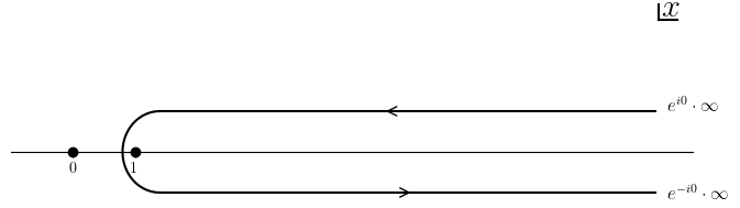
Figure 2.1: Integral contour $C$

Now we evaluate the integral (2.25) for $A_{r}^{(1)}$ with general $r$. Let us compute the first nontrivial term $Q_{2}(x)$. Since there appear integrants of the form $p(x)^{a}x^{b}$ frequently, it is convenient to introduce the symbol $J(a,b)$:

$$J(a,b)\equiv\int_{C}\left(x^{hM}-1\right)^{a}x^{b}dx=-\frac{e^{\pi ia}2\pi i}{hM}\frac{\Gamma\left(-a-\frac{b+1}{hM}\right)}{\Gamma(-a)\Gamma\left(1-\frac{b+1}{hM}\right)},$$ (2.26)

where $\Gamma$ is the Gamma function. Using the formula $\Gamma(x+1)=x\Gamma(x)$, the integral satisfies the recurrence relation:

$$J(a+m,b+(hM)n)=e^{i\pi m}\frac{(\frac{b+1}{hM}+n)!(a+m+1)!(a+\frac{b+1}{hM}+1)!}{(a+m+\frac{b+1}{hM}+n+1)!(\frac{b+1}{hM})!(a+1)!}J(a,b,h;M).$$ (2.27)

After evaluating the integral of $S_{2}(x)$ in Eq.(2.24), there are three integrals. According to the recurrence relation (2.26), they are combined into the following form.

$$Q_{2}= \frac{L_{2}}{h}J(-\frac{1}{h},-2)-\frac{(h^{2}-1)M(hM-1)}{12}J(-\frac{1}{h}-1,-2+hM)$$

$$+ \frac{(h^{2}-1)(2h+1)M^{2}}{24}J(-\frac{1}{h}-2,-2+2hM)$$

$$= \frac{1}{h}J(-\frac{1}{h},-2)\Big{(}L_{2}+\frac{1}{24}(h-1)h(hM-1)\Big{)}.$$

This construction rule can be applied to higher orders. For general $Q_{i}(x)$ case, there are $J(a+m,b+(hM)n)$ contained with two integers $0\leq m,n\leq i$. Thanks to the recurrence relation and the construction rule above, it is possible to design an algorithm to compute general $Q_{i}$. Let us list the first five nontrivial terms here, and the $6\text{th}$, $7\text{th}$ and $8\text{th}$ terms in Appendix A.

$$\begin{split}Q_{2}&=\frac{1}{h}J_{1,2}\Big{(}L_{2}+\frac{1}{24}(h-1)h(hM-1)\Big{)},\\ Q_{3}&=\frac{1}{h}J_{2,3}\Big{(}-L_{3}-(h-2)L_{2}\Big{)},\\ Q_{4}&=\frac{1}{h}J_{3,4}\Big{(}L_{4}+(h-3)\{-\frac{1}{2h}L_{2}^{2}+\frac{3}{2}L_{3}-\frac{1}{8}[h(M-4)+9]L_{2}\\ &\quad+\frac{1}{1920}(h-1)[hM-3][hM-1][2h(M+1)-1]\}\Big{)},\\ Q_{5}&=\frac{1}{h}J_{4,5}\Big{(}-L_{5}+\frac{1}{3h}(h-4)\{3L_{2}L_{3}+3(h-2)L_{2}^{2}-6L_{4}\\ &\quad+[h(M-3)+11]L_{3}+(h-2)(hM+2)L_{2}\}\Big{)},\end{split}$$ (2.28)

where $L_{k}$ vanishes when $k>h$ and $J(-n/h,m)$ are abbreviated to $J_{n,m}$ for convenience. We can check that $Q_{(1+hk)}$ ($k\in\mathbf{Z}$) becomes zero, which is consistent with the WKB analysis.

The WKB analysis of the $D_{r}^{(1)}$ type

We want to generalize the WKB analysis for $A_{r}^{(1)}$-type linear problem to that associated with the $\hat{\mathfrak{g}}$-type affine Toda field equations has been studied by diagonalization via gauge transformation in [27]. This subsection focuses on the $D_{r}^{(1)}$-type equation, and other types will be studied in a separate paper. Let us consider the $D_{r}^{(1)}$-type linear problem with (2.10) for the vector representation. The weight vector of the representation are $\epsilon_{1},\dots,\epsilon_{r},-\epsilon_{r},\dots,-\epsilon_{1}$, where $\epsilon_{i}$ are orthonormal basis with $\epsilon_{i}\cdot\epsilon_{j}=\delta_{ij}$. The simple roots are $\alpha_{i}=\epsilon_{1}-\epsilon_{i+1}$ ($i=1,\dots,r-1$) and $\alpha_{r}=\epsilon_{r}+\epsilon_{r-1}$. The Weyl vector $\rho=\sum_{i=1}^{r}(r-i)\epsilon_{i}$.

The linear problem reduces to the single differential equation for the component $\psi$ corresponding to the highest weight $\epsilon_{1}$ [29]:

$$\epsilon^{2r-2}\left(\partial_{x}-\frac{l_{1}}{x}\right)\cdots\left(\partial_{x}-\frac{l_{r}}{x}\right)\partial_{x}^{-1}\left(\partial_{x}+\frac{l_{r}}{x}\right)\cdots\left(\partial_{x}+\frac{l_{1}}{x}\right)\psi=4\sqrt{p(x)}\partial_{x}\sqrt{p(x)}\psi,$$ (2.29)

with $l_{k}=\epsilon_{k}\cdot l$ and $h=2r-2$ in $D_{r}^{(1)}$.

The ODE (2.29) is difficult to solve directly with the WKB method due to the existence of a pseudo-differential operator. However, when we start from the equivalent linear problem (2.15), its WKB solution is found by the diagonalization with gauge transformation [28]. Especially for the $D_{r}^{(1)}$-type linear problem in the vector representation, the diagonalized connection is characterized by the two functions: $f(x,\epsilon)$ and $K(x,\epsilon)$ [27]. The Riccati equations for $f(x,\epsilon)$ and $K(x,\epsilon)$ determine the WKB solution of the linear problem. Based on this diagonalization method, the WKB solutions to the $D_{3}^{(1)}$ and $D_{4}^{(1)}$ linear problems were found. The diagonalization method supports the following prescription to obtain the WKB series $f(x,\epsilon)$ based on an embedding of $B_{r-1}^{(1)}$ into $D_{r}^{(1)}$.

First, we set $l_{r}$ to be zero, by which the pseudo-ODE (2.29) reduces to the $B_{r-1}^{(r)}$-type ODE:

$$\epsilon^{2r-2} \left(\partial_{x}-\frac{l_{1}}{x}\right)\cdots\left(\partial_{x}-\frac{l_{r-1}}{x}\right)\partial_{x}\left(\partial_{x}+\frac{l_{r-1}}{x}\right)\cdots\left(\partial_{x}+\frac{l_{1}}{x}\right)\psi(x)$$

$$-4\sqrt{p(x)}\partial_{x}\sqrt{p(x)}\psi(x)=0.$$ (2.30)

The WKB expansion of this ODE can be studied as in the $A_{r}^{(1)}$ case. Expanding the differential operator in (2.1) such as

$$\left(\partial_{x}-\frac{l_{1}}{x}\right)\cdots\left(\partial_{x}-\frac{l_{r-1}}{x}\right)\partial_{x}\left(\partial_{x}+\frac{l_{r-1}}{x}\right)\cdots\left(\partial_{x}+\frac{l_{1}}{x}\right) =\partial^{2r-1}_{x}+\sum_{k=2}^{2r-1}\frac{L^{\prime}_{k}}{x^{k}}\partial^{2r-1-k}_{x},$$ (2.31)

and substituting (2.20) into (2.1), we obtain the Riccati equation:

$$(\epsilon\partial_{x}+S)^{2r-2}S+\sum_{i=2}^{2r-1}\frac{L^{\prime}_{i}}{x^{i}}(\epsilon\partial_{x}+S)^{2r-2-i}S-4\sqrt{p(z)}\partial_{z}\sqrt{p(z)}=0.$$ (2.32)

The Riccati equation can be solved recursively as

$$S_{0}(x) =2^{\frac{2}{h}}p(x)^{\frac{1}{h}},$$

$$S_{1}(x) =-\frac{1}{2}\partial_{x}\log(p),$$

$$S_{2}(x) =-4^{-1/h}\frac{L^{\prime}_{2}}{h}p^{-\frac{1}{h}}x^{-2}-2^{-\frac{2}{h}-3}\frac{(h+1)(h+2)(2h+1)M^{2}}{3}p^{-\frac{1}{h}-2}x^{-2+2hM}$$

$$+\frac{4^{-\frac{h+1}{h}}(h+1)(h+2)(hM-1)M}{3h}p^{-\frac{1}{h}-1}x^{-2+hM},$$ (2.33)

where $h=2r-2$. The parameters $L^{\prime}_{k}$ in (2.31) are shown to be symmetric polynomials of $(\epsilon_{1},l+\rho)^{2},\dots,(\epsilon_{r-1},l+\rho)^{2}$. It is observed that the WKB expansion $f(x,\epsilon)$ for $D_{r}^{(1)}$ can be obtained by promoting $L_{k}^{\prime}$ to the symmetric polynomial of the same order by adding $(\epsilon_{r},l+\rho)^{2}$. Explicitly, the first five $L^{\prime}_{k}$ for $D_{r}^{(1)}$ are given by

$$\begin{split}L^{\prime}_{2}=&-s_{1}+\frac{1}{12}(2r-1)r(2r-2),\\ L^{\prime}_{3}=&-(2r-3)L^{\prime}_{2},\\ L^{\prime}_{4}=&s_{2}-\frac{1}{6}(r-2)(r+11)(2r-3)s_{1}\\ +&\frac{1}{360}(r-2)(r-1)r(2r-3)(2r-1)(5r+109),\\ L^{\prime}_{5}=&(10-4r)L^{\prime}_{4}+2(r-2)(2r-5)(2r-3)L^{\prime}_{2},\\ L^{\prime}_{6}=&-s_{3}+\frac{1}{6}(r-3)(r+34)(2r-5)s_{2}\\ -&\frac{1}{360}(r-3)(r-2)(2r-5)(2r-3)(5r^{2}+339r+1096)s_{1}\\ +&\frac{1}{45360}(r-3)(r-2)(r-1)r(2r-1)(2r-3)(2r-5)(35r^{2}+3549r+22306),\end{split}$$ (2.34)

and $s_{k}$ is defined by

$$s_{k}=\sum_{1\leq i_{1}<i_{2}<\dots<i_{k}\leq r}(\epsilon_{i_{1}},l+\rho)^{2}(\epsilon_{i_{2}},l+\rho)^{2}\dots(\epsilon_{i_{k}},l+\rho)^{2}.$$

The diagonal element $K(x,\epsilon)$ provides another WKB solution whose leading term is given by $2p^{-\frac{1}{2}}x^{-r}K_{r}$ where

$$K_{r}:=x^{r}\left(\partial_{x}-\frac{l_{1}}{x}\right)\cdots\left(\partial_{x}-\frac{l_{r}}{x}\right)\cdot 1=(\epsilon_{1},l+\rho)\cdots(\epsilon_{r},l+\rho).$$ (2.35)

Note that $s_{1},\dots,s_{r-1},K_{r}$ characterize the Casimir invariants of $D_{r}$. After substituting these diagonal elements into Eq.(2.25), we can obtain the first five ($Q_{6}$ can be found in the Appendix A) and the extra WKB integrals:

$$\begin{split}Q_{2}&=-\frac{2^{-\frac{2}{h}}}{h}J_{1,2}\left(L^{\prime}_{2}+\frac{1}{24}h(h+2)(hM-1)\right),\\ Q_{3}&=-\frac{2^{-\frac{4}{h}}}{h}J_{2,3}\left[L^{\prime}_{3}+(2r-3)L^{\prime}_{2}\right]=0,\\ Q_{4}&=-\frac{2^{-\frac{6}{h}}}{h}J_{3,4}\bigg{[}L^{\prime}_{4}-\frac{h-3}{2h}L_{2}^{{}^{\prime}2}+\frac{3(h-2)}{2}L^{\prime}_{3}\\ &-\frac{1}{8}\left[(M-4)h^{2}-(6M-9)h-6\right]L^{\prime}_{2}\\ &+\frac{1}{1920}h(h-6)(h+2)(Mh-3)(Mh-1)(2(M+1)h-1)\bigg{]},\\ Q_{5}&=-\frac{2^{-\frac{8}{h}}}{h}J_{4,5}\bigg{[}L^{\prime}_{5}+\frac{4}{h}L^{\prime}_{2}L^{\prime}_{3}+2(h-3)L^{\prime}_{4}-\frac{(h-4)(h-1)}{h}L_{2}^{{}^{\prime}2}\\ &+\frac{1}{6}\left(40-28h+6h^{2}+(11-2h)hM\right)L^{\prime}_{3}\\ &-\frac{1}{6}(h-1)\left((2h-11)hM-2(h+2)\right)L^{\prime}_{2}\bigg{]},\\ Q^{\prime}_{r}&=2J(-\frac{1}{2},-r)(\epsilon_{1},l_{1}+\rho)\cdots(\epsilon_{1},l_{r}+\rho),\\ \end{split}$$ (2.36)

where $L^{\prime}_{k}$ also vanishes when $k>h$.

Above all, we have obtained the period integrals of the WKB solutions or charges of the classical conserved currents in modified affine Toda field theories. In the next section, we compute the quantum IoMs in CFT with $W$-symmetry.

3 Conformal field theory with $W$ symmetry

In this section, we will review two-dimensional CFT with $W$-symmetry and its free field representation. For more details about the $W$ algebra, see a review [13]. We will then compute the quantum IoMs on the cylinder.

We first consider CFT on a complex plane. Let $(z,\bar{z})$ be a complex coordinate on the complex plane. A CFT is completely characterized by a set of operators and their operator product expansions (OPE). An operator $A(z,\bar{z})$ in CFT is decomposed into the holomorphic part $A(z)$ and the anti-holomorphic part $\bar{A}(\bar{z})$. We focus on the holomorphic part.

Conformal transformation is generated by the energy-momentum tensor $T(z)$, whose OPE is given by

$$T(z)T(w)=\frac{c/2}{(z-w)^{4}}+\frac{2T(w)}{(z-w)^{2}}+\frac{\partial_{w}T(w)}{z-w}+\cdots,$$ (3.1)

where $c$ is the central charge. The term $\dots$ denotes the regular terms. The primary field $\Phi(z)$ with conformal dimension $\Delta$ is defined by the OPE

$$T(z)\Phi(w)=\frac{\Delta\Phi(w)}{(z-w)^{2}}+\frac{\partial_{w}\Phi_{(}w)}{z-w}+\cdots,$$ (3.2)

The symmetry algebra of a CFT can be extended by adding currents. In particular, the algebra generated by higher spin currents is called the $W$ algebra. Let $W_{s}(z)$ denote the spin $s$ current. Note that $T(z)$ is a spin 2 current: $W_{2}(z)=T(z)$.

Let $A(z)$ and $B(z)$ be two symmetry generators with conformal dimension $\Delta_{A}$ and $\Delta_{B}$, respectively. The operator product expansion takes the form

$$A(z)B(w)=\sum_{1\leq k\leq\Delta_{A}+\Delta_{b}}\frac{\{AB\}_{k}(w)}{(z-w)^{k}}+\savestack\Tmp{\raisebox{-0.7pt}{$\ensurestackMath{\stackon[0.5ex]{\circ}{\circ}}$}}\Tmpcontent=\Tmpcontent-.7pt\mathrel{\scalerel*{\Tmp}{:}}AB\savestack\Tmp{\raisebox{-0.7pt}{$\ensurestackMath{\stackon[0.5ex]{\circ}{\circ}}$}}\Tmpcontent=\Tmpcontent-.7pt\mathrel{\scalerel*{\Tmp}{:}}(w)+O(z-w).$$ (3.3)

Here $\savestack\Tmp{\raisebox{-0.7pt}{$\ensurestackMath{\stackon[0.5ex]{\circ}{\circ}}$}}\Tmpcontent=\Tmpcontent-.7pt\mathrel{\scalerel*{\Tmp}{:}}AB\savestack\Tmp{\raisebox{-0.7pt}{$\ensurestackMath{\stackon[0.5ex]{\circ}{\circ}}$}}\Tmpcontent=\Tmpcontent-.7pt\mathrel{\scalerel*{\Tmp}{:}}(w)$ is the normal ordered product on the complex plane defined by the radial ordered product:

$$\savestack\Tmp{\raisebox{-0.7pt}{$\ensurestackMath{\stackon[0.5ex]{\circ}{\circ}}$}}\Tmpcontent=\Tmpcontent-.7pt\mathrel{\scalerel*{\Tmp}{:}}AB\savestack\Tmp{\raisebox{-0.7pt}{$\ensurestackMath{\stackon[0.5ex]{\circ}{\circ}}$}}\Tmpcontent=\Tmpcontent-.7pt\mathrel{\scalerel*{\Tmp}{:}}(w)={1\over 2\pi i}\oint dz{R(A(z)B(w))\over z-w}.$$ (3.4)

3.1 Free field realization of W-algebras

We will define the $W$-algebra by the free field realizations. For $A_{r}$ and $D_{r}$ type $W$-algebras, their free field realization can be obtained by the quantum Miura transformation [37, 38]. The EM tensor and higher spin $W$ currents are obtained from polynomials of the scalar field $\phi(z)$ and their derivatives. These are also regarded as quantized symmetry of non-affine Toda field theories of (2.1). The OPE of $\phi_{i}(z)$ is defined by

$$\phi_{i}(z)\phi_{j}(w)=-\delta_{ij}\log(z-w)+\cdots.$$ (3.5)

The mode expansion of $\partial\phi_{j}(z)$

$$i\partial\phi_{j}(z) =\sum_{n\in{\mathbb{Z}}}a_{n}^{j}z^{-n-1},$$ (3.6)

leads to the commutation relations of $a^{j}_{n}$: $[a^{i}_{n},a^{j}_{m}]=n\delta_{n+m,0}\delta^{ij}$. The EM tensor in the $W{\mathfrak{g}}$-algebra with simply-laced Lie algebra ${\mathfrak{g}}$ is defined by

$$T(z) =-{1\over 2}\savestack\Tmp{\raisebox{-0.7pt}{$\ensurestackMath{\stackon[0.5ex]{\circ}{\circ}}$}}\Tmpcontent=\Tmpcontent-.7pt\mathrel{\scalerel*{\Tmp}{:}}(\partial_{z}\phi)^{2}(z)\savestack\Tmp{\raisebox{-0.7pt}{$\ensurestackMath{\stackon[0.5ex]{\circ}{\circ}}$}}\Tmpcontent=\Tmpcontent-.7pt\mathrel{\scalerel*{\Tmp}{:}}-i\alpha_{0}\rho\cdot\partial^{2}_{z}\phi(z),$$ (3.7)

whose central charge is given by

$$c =r-12\alpha_{0}^{2}\rho^{2}.$$ (3.8)

We also define a vertex operator

$$V_{\Lambda}(z)=\savestack\Tmp{\raisebox{-0.7pt}{$\ensurestackMath{\stackon[0.5ex]{\circ}{\circ}}$}}\Tmpcontent=\Tmpcontent-.7pt\mathrel{\scalerel*{\Tmp}{:}}e^{i\Lambda\cdot\phi(z)}\savestack\Tmp{\raisebox{-0.7pt}{$\ensurestackMath{\stackon[0.5ex]{\circ}{\circ}}$}}\Tmpcontent=\Tmpcontent-.7pt\mathrel{\scalerel*{\Tmp}{:}}\;,$$ (3.9)

which is a primary field with conformal weight $\Delta_{\Lambda}={1\over 2}\Lambda(\Lambda+2\alpha_{0}\rho)$.

Free field realization of $WA_{r}$ algebra

The $WA_{r}$ algebra is generated by spin $2,\dots,r+1$ currents. The quantum Miura transformation [37] is a method to obtain their free field realization:

$$(\alpha_{0}\partial_{z})^{r+1}-\sum_{k=2}^{r+1}\tilde{W}_{k}(z)\left(\alpha_{0}\partial_{z}\right)^{h-k}=\savestack\Tmp{\raisebox{-0.7pt}{$\ensurestackMath{\stackon[0.5ex]{\circ}{\circ}}$}}\Tmpcontent=\Tmpcontent-.7pt\mathrel{\scalerel*{\Tmp}{:}}\left(\alpha_{0}\partial_{z}-\epsilon_{1}\cdot i\partial_{z}\phi\right)\ldots\left(\alpha_{0}\partial_{z}-\epsilon_{r+1}\cdot i\partial_{z}\phi\right)\savestack\Tmp{\raisebox{-0.7pt}{$\ensurestackMath{\stackon[0.5ex]{\circ}{\circ}}$}}\Tmpcontent=\Tmpcontent-.7pt\mathrel{\scalerel*{\Tmp}{:}}(z)\;.$$ (3.10)

Here spin 2 and 3 $W$ currents are given as

$$\begin{split}\tilde{W}_{2}(z)&=-\frac{1}{2}\savestack\Tmp{\raisebox{-0.7pt}{$\ensurestackMath{\stackon[0.5ex]{\circ}{\circ}}$}}\Tmpcontent=\Tmpcontent-.7pt\mathrel{\scalerel*{\Tmp}{:}}(\partial_{z}\phi\cdot\partial_{z}\phi)\savestack\Tmp{\raisebox{-0.7pt}{$\ensurestackMath{\stackon[0.5ex]{\circ}{\circ}}$}}\Tmpcontent=\Tmpcontent-.7pt\mathrel{\scalerel*{\Tmp}{:}}(z)-i\alpha_{0}\rho\cdot\partial_{z}^{2}\phi(z),\\ \tilde{W}_{3}(z)&=\sum_{i<j<k}\savestack\Tmp{\raisebox{-0.7pt}{$\ensurestackMath{\stackon[0.5ex]{\circ}{\circ}}$}}\Tmpcontent=\Tmpcontent-.7pt\mathrel{\scalerel*{\Tmp}{:}}\left(\epsilon_{i}\cdot i\partial_{z}\phi\right)\left(\epsilon_{j}\cdot i\partial_{z}\phi\right)\left(\epsilon_{k}\cdot i\partial_{z}\phi\right)\savestack\Tmp{\raisebox{-0.7pt}{$\ensurestackMath{\stackon[0.5ex]{\circ}{\circ}}$}}\Tmpcontent=\Tmpcontent-.7pt\mathrel{\scalerel*{\Tmp}{:}}(z)\\ -&\alpha_{0}\sum_{i<j}(i-1)\partial_{z}\savestack\Tmp{\raisebox{-0.7pt}{$\ensurestackMath{\stackon[0.5ex]{\circ}{\circ}}$}}\Tmpcontent=\Tmpcontent-.7pt\mathrel{\scalerel*{\Tmp}{:}}\left(\epsilon_{i}\cdot i\partial_{z}\phi\right)\left(\epsilon_{j}\cdot i\partial_{z}\phi\right)\savestack\Tmp{\raisebox{-0.7pt}{$\ensurestackMath{\stackon[0.5ex]{\circ}{\circ}}$}}\Tmpcontent=\Tmpcontent-.7pt\mathrel{\scalerel*{\Tmp}{:}}(z)\\ -&\alpha_{0}\sum_{i<j}(j-i-1)\savestack\Tmp{\raisebox{-0.7pt}{$\ensurestackMath{\stackon[0.5ex]{\circ}{\circ}}$}}\Tmpcontent=\Tmpcontent-.7pt\mathrel{\scalerel*{\Tmp}{:}}\left(\epsilon_{i}\cdot i\partial_{z}\phi\right)\left(\epsilon_{j}\cdot i\partial_{z}^{2}\phi\right)\savestack\Tmp{\raisebox{-0.7pt}{$\ensurestackMath{\stackon[0.5ex]{\circ}{\circ}}$}}\Tmpcontent=\Tmpcontent-.7pt\mathrel{\scalerel*{\Tmp}{:}}(z)+\frac{1}{2}\alpha_{0}^{2}\sum_{i}(i-1)(i-2)\left(\epsilon_{i}\cdot i\partial_{z}^{3}\phi\right)(z).\end{split}$$ (3.11)

Here $h=r+1$ and $\rho=\sum_{i=1}^{r}(r+1-i)\epsilon_{i}$. The current $\tilde{W}_{2}(z)$ is nothing but the energy-momentum tensor $T(z)$, which leads to the central charge

$$c =r-r(r+1)(r+2)\alpha_{0}^{2}.$$ (3.12)

Their OPE can be computed from the OPE (3.5). In general, the spin $k$ current $\tilde{W}_{k}(z)$ is not the primary field. But we can redefine these fields into primary fields denoted by $W_{k}(z)$. Computing the OPEs in lower rank $WA_{r}$-algebras, it is possible to infer the primary $W$-currents:

$$\begin{split}&T(z)=\tilde{W}_{2}(z),\\ &W_{3}(z)=\tilde{W}_{3}(z)-\frac{h-2}{2}\alpha_{0}\partial_{z}T(z),\\ &W_{4}(z)=\tilde{W}_{4}(z)+(h-3)\left(x_{1}\savestack\Tmp{\raisebox{-0.7pt}{$\ensurestackMath{\stackon[0.5ex]{\circ}{\circ}}$}}\Tmpcontent=\Tmpcontent-.7pt\mathrel{\scalerel*{\Tmp}{:}}TT\savestack\Tmp{\raisebox{-0.7pt}{$\ensurestackMath{\stackon[0.5ex]{\circ}{\circ}}$}}\Tmpcontent=\Tmpcontent-.7pt\mathrel{\scalerel*{\Tmp}{:}}(z)-\frac{1}{2}\alpha_{0}\partial_{z}\tilde{W}_{3}(z)-x_{2}\partial_{z}^{2}T(z)\right),\\ &W_{5}(z)=\tilde{W}_{5}(z)-{r-3\over 2}\alpha_{0}\partial_{z}\tilde{W}_{4}(z)+y_{1}\savestack\Tmp{\raisebox{-0.7pt}{$\ensurestackMath{\stackon[0.5ex]{\circ}{\circ}}$}}\Tmpcontent=\Tmpcontent-.7pt\mathrel{\scalerel*{\Tmp}{:}}TW_{3}\savestack\Tmp{\raisebox{-0.7pt}{$\ensurestackMath{\stackon[0.5ex]{\circ}{\circ}}$}}\Tmpcontent=\Tmpcontent-.7pt\mathrel{\scalerel*{\Tmp}{:}}(z)+y_{2}\partial_{z}^{2}W_{3}(z)+y_{3}\alpha_{0}\partial_{z}^{3}T(z),\end{split}$$ (3.13)

with

$$\begin{split}&x_{1}=\frac{(h-2)((5h+7)c-2h+2)}{2(5c+22)h\left(h+1\right)\left(h-1\right)},\quad x_{2}=\frac{(h-2)(2c^{2}+(h+15)c-10(h-1))}{4(5c+22)h\left(h+1\right)\left(h-1\right)},\\ &y_{1}=\frac{(h-4)(h-3)((7h+13)c-6h+6)}{(7c+114)h\left(h+1\right)\left(h-1\right)},\\ &y_{2}=-\frac{3(h-4)(h-3)(c^{2}+(h+21)c-18(h-1))}{4(7c+114)h\left(h+1\right)\left(h-1\right)},\\ &y_{3}=\frac{(h-4)(h-3)\left((32-7h)c^{2}+(7h^{2}-117h+620)c+6(h-1)(19h-92)\right)}{24(7c+114)h\left(h+1\right)\left(h-1\right)}.\end{split}$$ (3.14)

Applying the differential operator (3.10) to the vertex operator $V_{\Lambda}(z)$, one obtains the formula for conformal weight of $\tilde{W}_{k}(z)$ [4]:

$$\tilde{\Delta}_{k} =(-1)^{k-1}\sum_{i_{1}<i_{2}<\dots<i_{k}}\prod_{j=1}^{k}\left[p_{i_{j}}+\left((k-j)-\frac{1}{2}(r+2-2i_{j})\right)\alpha_{0}\right],$$ (3.15)

where the new parameter $p$ is given by a shift of $\Lambda$

$$\quad p=\Lambda+\alpha_{0}\rho^{\vee},\quad p_{i}=(\epsilon_{i},p).$$ (3.16)

The conformal weights $\tilde{\Delta}_{i}$ for $i=2,3,4$ and 5 are given by

$$\begin{split}\tilde{\Delta}_{2}&=-\sigma_{2}-\frac{1}{4}\binom{n+2}{3}\alpha_{0}^{2},\\ \tilde{\Delta}_{3}&=\sigma_{3}+(r-1)\alpha_{0}\sigma_{2}+\binom{r+2}{4}\alpha_{0}^{3},\\ \tilde{\Delta}_{4}&=-\sigma_{4}-\frac{3}{2}\left(r-2\right)\alpha_{0}\sigma_{3}-\frac{1}{24}(r-2)(r-1)(r+24)\alpha_{0}^{2}\sigma_{2}\\ &\quad-\frac{1}{5760}(r-2)(r-1)r(r+1)(r+2)(5r+228)\alpha_{0}^{4},\\ \tilde{\Delta}_{5}&=\sigma_{5}+2(r-3)\alpha_{0}\sigma_{4}+\frac{1}{24}(r-3)(r-2)(r+44)\alpha_{0}^{2}\sigma_{3}\\ &\quad+\frac{1}{12}(r-3)(r-2)(r-1)(r+12)\alpha_{0}^{3}\sigma_{2}\\ &\quad+\frac{1}{2880}(r-3)(r-2)(r-1)r(r+1)(r+2)(5r+108)\alpha_{0}^{5},\end{split}$$ (3.17)

where we define

$$\sigma_{k}=\sum_{1\leq i_{1}<i_{2}<\dots<i_{k}\leq r+1}p_{i_{1}}p_{i_{2}}\dots p_{i_{k}}.$$ (3.18)

The relations between conformal weights $\Delta_{i}$ of primary $W_{k}(z)$ and $\tilde{\Delta}_{i}$ can be derived from Eq.(3.13). One finds that

$$\begin{split}\Delta_{2}&=\tilde{\Delta}_{2},\\ \Delta_{3}&=\tilde{\Delta}_{3}+(h-2)\alpha_{0}\Delta_{2},\\ \Delta_{4}&=\tilde{\Delta}_{4}+(h-3)\left(c_{4}^{(1)}\Delta_{2}^{2}+\frac{3}{2}\alpha_{0}\tilde{\Delta}_{3}+c_{4}^{(2)}\Delta_{2}\right),\\ \Delta_{5}&=\tilde{\Delta}_{5}+(h-4)\left(c_{5}^{(1)}\Delta_{2}\Delta_{3}+2\alpha_{0}\tilde{\Delta}_{4}+c_{5}^{(2)}\Delta_{3}-(h-3)(h-2)\alpha_{0}^{2}\Delta_{2}\right)\end{split}$$ (3.19)

with the coefficients

$$\begin{split}&c_{4}^{(1)}=\frac{(h-2)[(5h+7)c-2h+2]}{2(5c+22)h\left(h+1\right)\left(h-1\right)},\quad c_{4}^{(2)}=-\frac{(h-2)[6c^{2}-(7h-31)c-26(h-1)]}{2(5c+22)h\left(h+1\right)\left(h-1\right)},\\ &c_{5}^{(1)}=\frac{(h-3)[(7h+13)c-6h+6]}{(7c+114)h\left(h+1\right)\left(h-1\right)},\quad c_{5}^{(2)}=-\frac{3(h-3)\left[3c^{2}-4(c+12)h+50c+48\right]}{(7c+114)h\left(h+1\right)\left(h-1\right)}.\end{split}$$

Free field realization of $WD_{r}$ algebra

The $WD_{r}$ algebra contains spin $2,4,\dots,2r-2$ currents $\{W_{2},W_{4},\dots,W_{2r-2}\}$ and the spin $r$ current $R_{r}$. The free field realization of the spin $r$ current is defined by [38]:

$$R_{r}(z)=\savestack\Tmp{\raisebox{-0.7pt}{$\ensurestackMath{\stackon[0.5ex]{\circ}{\circ}}$}}\Tmpcontent=\Tmpcontent-.7pt\mathrel{\scalerel*{\Tmp}{:}}\left(\alpha_{0}\partial_{z}-i\epsilon_{1}\cdot\partial_{z}\phi(z)\right)\ldots\left(\alpha_{0}\partial_{z}-i\epsilon_{n}\cdot\partial_{z}\phi(z)\right)\savestack\Tmp{\raisebox{-0.7pt}{$\ensurestackMath{\stackon[0.5ex]{\circ}{\circ}}$}}\Tmpcontent=\Tmpcontent-.7pt\mathrel{\scalerel*{\Tmp}{:}}\cdot 1.$$ (3.20)

Here $\epsilon_{1},\dots,\epsilon_{r}$ are the orthonormal basis of ${\mathbb{R}}^{r}$. The other $W$ currents are determined by the OPE of $R_{r}$:

$$R_{r}(z)R_{r}(w)=\frac{A_{r}}{(z-w)^{2r}}+\sum_{k=1}^{r-1}\frac{A_{r-k}}{(z-w)^{2(r-k)}}\left(\tilde{W}_{2k}(z)+\tilde{W}_{2k}(w)\right),$$ (3.21)

where

$$A_{k}=\prod_{j=1}^{k-1}(1-2j(2j+1)\alpha_{0}^{2}).$$ (3.22)

The energy-momentum tensor $T(z)$ is given by $\tilde{W}_{2}(z)$:

$$\tilde{W}_{2}(z) =-{1\over 2}\savestack\Tmp{\raisebox{-0.7pt}{$\ensurestackMath{\stackon[0.5ex]{\circ}{\circ}}$}}\Tmpcontent=\Tmpcontent-.7pt\mathrel{\scalerel*{\Tmp}{:}}(\partial_{z}\phi\cdot\partial_{z}\phi)\savestack\Tmp{\raisebox{-0.7pt}{$\ensurestackMath{\stackon[0.5ex]{\circ}{\circ}}$}}\Tmpcontent=\Tmpcontent-.7pt\mathrel{\scalerel*{\Tmp}{:}}(z)-i\alpha_{0}\rho\cdot\partial_{z}^{2}\phi(z)$$ (3.23)

with $\rho=\sum_{i=1}^{r}(r-i)\epsilon_{i}$. The central charge is

$$c =r-r(2r-1)(2r-2)\alpha_{0}^{2}.$$ (3.24)

The free field realization of $\tilde{W}_{2k}$ can also be obtained from (3.21), which are non-primary, while $R_{r}$ is a primary field. Here we will construct $\tilde{W}_{4}$ and $\tilde{W}_{6}$ recursively as follows. First, we note that $WD_{r}$ CFT is obtained by adding a free boson to $WD_{r-1}$:

$$WD_{r}=\{\tilde{\phi}_{r}\}\oplus WD_{r-1}$$ (3.25)

with $\tilde{\phi}_{i}=\epsilon_{r+1-i}\cdot\phi$. Let $W_{2}^{(r)},\dots,W^{(r)}_{2r-2},R^{(r)}_{r}$ be generators of the $WD_{r}$ algebra. Then $R_{r}^{(r)}$ is related to $R^{(r-1)}_{r-1}$ via

$$R^{(r)}_{r}=-\savestack\Tmp{\raisebox{-0.7pt}{$\ensurestackMath{\stackon[0.5ex]{\circ}{\circ}}$}}\Tmpcontent=\Tmpcontent-.7pt\mathrel{\scalerel*{\Tmp}{:}}\tilde{p}_{r}R^{(r-1)}_{r-1}\savestack\Tmp{\raisebox{-0.7pt}{$\ensurestackMath{\stackon[0.5ex]{\circ}{\circ}}$}}\Tmpcontent=\Tmpcontent-.7pt\mathrel{\scalerel*{\Tmp}{:}}+\alpha_{0}\partial R_{r-1}^{(r-1)},\quad\tilde{p}_{r}=-i\partial\tilde{\phi}_{r}.$$ (3.26)

This implies that the OPE $R_{r}^{(r)}(z)R_{r}^{(r)}(w)$ is obtained from $R_{r-1}^{(r-1)}(z)R^{(r-1)}_{r-1}(w)$, which leads to the recursion relations for $W_{2k}^{(r)}$. An explicit calculation is shown in the Appendix B. Thus we obtain the non-primary $W$-currents $\tilde{W}_{4}$. The primary $W_{4}$ current is given by

$$\begin{split}W_{4}(z)&=\tilde{W}_{4}(z)+a_{1}\savestack\Tmp{\raisebox{-0.7pt}{$\ensurestackMath{\stackon[0.5ex]{\circ}{\circ}}$}}\Tmpcontent=\Tmpcontent-.7pt\mathrel{\scalerel*{\Tmp}{:}}TT\savestack\Tmp{\raisebox{-0.7pt}{$\ensurestackMath{\stackon[0.5ex]{\circ}{\circ}}$}}\Tmpcontent=\Tmpcontent-.7pt\mathrel{\scalerel*{\Tmp}{:}}(z)+a_{2}\partial_{z}^{2}T(z)\end{split}$$ (3.27)

with the coefficients

$$a_{1} =-{5r+1\over 22+5c}\left(1-2(r-2)(2r-3)\alpha_{0}^{2}\right),$$

$$a_{2} ={1\over 22+5c}\left(1-2(r-2)(2r-3)\alpha_{0}^{2}\right)\left({4r+5\over 2}-r(r-1)(2r-1)\alpha_{0}^{2}\right).$$ (3.28)

There is no explicit formula for conformal weight $\Delta_{i}$ in $WD_{r}$ algebras[38], but we can still summarize some lowest-order ones as follows:

$$\tilde{\Delta}_{2} ={1\over 2}\sigma_{1}-{r(2r-2)(2r-1)\over 24}\alpha_{0}^{2},$$ (3.29)

$$\tilde{\Delta}_{4} ={1\over 2}\sigma_{2}-\left({1\over 12}(r-7)(r-2)(2r-3)\alpha_{0}^{2}+{1\over 4}\right)\sigma_{1}+{r(2r-1)(r-1)\over 24}\alpha_{0}^{2}$$

$$+{1\over 720}(r-2)(r-1)r(2r-3)(2r-1)(5r-71)\alpha_{0}^{4},$$ (3.30)

where $\sigma_{i}$ is defined by

$$\sigma_{k}=\sum_{1\leq i_{1}<i_{2}<\dots<i_{k}\leq r}p_{i_{1}}^{2}p_{i_{2}}^{2}\dots p_{i_{k}}^{2}.$$ (3.31)

The relation between $\Delta_{4}$ of the primary $W_{4}(z)$ and $\tilde{\Delta}_{4}$ is expressed as

$$\Delta_{4}=\tilde{\Delta}_{4}+a_{1}\Delta_{2}^{2}+2(a_{1}+3a_{2})\Delta_{2},$$ (3.32)

where $a_{1}$ and $a_{2}$ is given in (3.28). Finally, the conformal weight for the extra generator $R_{r}$ is

$$\Delta^{\prime}_{r}=p_{1}p_{2}\cdots p_{r}.$$ (3.33)

For $\Delta_{6}$, so far, we can only give its value in $WD_{4}$ algebra. The primary spin 6 current $W_{6}$ is given by

$$\begin{split}W_{6}&=\tilde{W}_{6}-{1\over 3}\savestack\Tmp{\raisebox{-0.7pt}{$\ensurestackMath{\stackon[0.5ex]{\circ}{\circ}}$}}\Tmpcontent=\Tmpcontent-.7pt\mathrel{\scalerel*{\Tmp}{:}}T\tilde{W}_{4}\savestack\Tmp{\raisebox{-0.7pt}{$\ensurestackMath{\stackon[0.5ex]{\circ}{\circ}}$}}\Tmpcontent=\Tmpcontent-.7pt\mathrel{\scalerel*{\Tmp}{:}}-{-13+1388\alpha_{0}^{2}-22560\alpha_{0}^{4}\over 84(4-241\alpha_{0}^{2}+2352\alpha_{0}^{4})}\savestack\Tmp{\raisebox{-0.7pt}{$\ensurestackMath{\stackon[0.5ex]{\circ}{\circ}}$}}\Tmpcontent=\Tmpcontent-.7pt\mathrel{\scalerel*{\Tmp}{:}}T(\savestack\Tmp{\raisebox{-0.7pt}{$\ensurestackMath{\stackon[0.5ex]{\circ}{\circ}}$}}\Tmpcontent=\Tmpcontent-.7pt\mathrel{\scalerel*{\Tmp}{:}}TT\savestack\Tmp{\raisebox{-0.7pt}{$\ensurestackMath{\stackon[0.5ex]{\circ}{\circ}}$}}\Tmpcontent=\Tmpcontent-.7pt\mathrel{\scalerel*{\Tmp}{:}})\savestack\Tmp{\raisebox{-0.7pt}{$\ensurestackMath{\stackon[0.5ex]{\circ}{\circ}}$}}\Tmpcontent=\Tmpcontent-.7pt\mathrel{\scalerel*{\Tmp}{:}}\\ &-{9-2992\alpha_{0}^{2}+70688\alpha_{0}^{4}-288960\alpha_{0}^{6}\over 168(4-241\alpha_{0}^{2}+2352\alpha_{0}^{4})}\savestack\Tmp{\raisebox{-0.7pt}{$\ensurestackMath{\stackon[0.5ex]{\circ}{\circ}}$}}\Tmpcontent=\Tmpcontent-.7pt\mathrel{\scalerel*{\Tmp}{:}}T\partial_{z}^{2}T\savestack\Tmp{\raisebox{-0.7pt}{$\ensurestackMath{\stackon[0.5ex]{\circ}{\circ}}$}}\Tmpcontent=\Tmpcontent-.7pt\mathrel{\scalerel*{\Tmp}{:}}\\ &-{23-815\alpha_{0}^{2}+6302\alpha_{0}^{4}+15960\alpha_{0}^{6}\over 84(4-241\alpha_{0}^{2}+2352\alpha_{0}^{4})}\savestack\Tmp{\raisebox{-0.7pt}{$\ensurestackMath{\stackon[0.5ex]{\circ}{\circ}}$}}\Tmpcontent=\Tmpcontent-.7pt\mathrel{\scalerel*{\Tmp}{:}}\partial T\partial T\savestack\Tmp{\raisebox{-0.7pt}{$\ensurestackMath{\stackon[0.5ex]{\circ}{\circ}}$}}\Tmpcontent=\Tmpcontent-.7pt\mathrel{\scalerel*{\Tmp}{:}}\\ &+{1-4\alpha_{0}^{2}\over 6}\partial^{2}\tilde{W}_{4}-{-2+425\alpha_{0}^{2}-10274\alpha_{0}^{4}+53496\alpha_{0}^{6}-40320\alpha_{0}^{8}\over 144(4-241\alpha_{0}^{2}+2352\alpha_{0}^{4})}\partial^{4}T,\\ \Delta_{6}&=\tilde{\Delta}_{6}-{1\over 3}\Delta_{2}\tilde{\Delta}_{4}+t_{3}\Delta_{2}^{3}+t_{4}\tilde{\Delta}_{4}+t_{5}\Delta_{2}^{2}+t_{6}\Delta_{2},\end{split}$$ (3.34)

with

$$t_{3} ={13-1388\alpha_{0}^{2}+22560\alpha_{0}^{4}\over 84(4-241\alpha_{0}^{2}+2352\alpha_{0}^{4})},$$

$$t_{4} =2-{40\alpha_{0}^{3}\over 3},$$

$$t_{5} ={-41+3908\alpha_{0}^{2}-101912\alpha_{0}^{4}+803040\alpha_{0}^{6}\over 84(4-241\alpha_{0}^{2}+2352\alpha_{0}^{4})},$$

$$t_{6} ={-1-30\alpha_{0}^{2}+6796\alpha_{0}^{4}-186480\alpha_{0}^{6}+1411200\alpha_{0}^{8}\over 42(4-241\alpha_{0}^{2}+2352\alpha_{0}^{4})}.$$

The expansion of $\tilde{\Delta}_{6}$ in terms of momentum becomes

$$\Delta_{6} ={1\over 2}\sigma_{3}+(-1+{11\over 2}\alpha_{0}^{2})\sigma_{2}+({1\over 2}-8a^{2}+{61\over 2}\alpha_{0}^{4})\sigma_{1}-7\alpha_{0}^{2}+161\alpha_{0}^{4}-{1429\alpha_{0}^{6}\over 2}.$$

3.2 Integrals of motion on a complex plane

The IoMs for relevant perturbation around CFT were studied in [11, 10, 12, 40]. The conserved currents that correspond to the generalized KdV flows are constructed by the OPE between the $W$-currents [5]. Toda field theories, as integrable models, possess an infinite number of IoMs.

On the complex plane, the IoMs can be given by the contour integral around the origin

$$\mathbf{M}_{k}=\frac{1}{2\pi i}\oint dz\;J_{k}(z).$$ (3.35)

Here $J_{k}(z)$ ($k\in{\bf Z}$) are the conserved currents, which can be constructed from normal ordered products of the EM tensor $T$, higher-spin $W$ fields, and their derivatives. $J_{k}(z)$ are uniquely determined up to the total derivative terms by the requirement of mutual commutativity condition:

$$[\mathbf{M}_{i},\mathbf{M}_{j}]=0,\quad\text{for}\;i,j\in\mathbf{Z}.$$ (3.36)

The explicit expressions of currents for Virasoro minimal models can be found in [11].

3.3 Integrals of motion on a cylinder

The IoMs obtained on a complex plane can be transformed into the ones on a cylinder by conformal transformation[1]. The zero mode of the conserved currents is necessary to see the correspondence between the ODE and the CFT. Due to the difference in the normal ordering prescriptions between complex plane and cylinder, the zero modes on the cylinder have non-trivial corrections. Some technical details for the Virasoso CFT have been developed in [3, 41]. Here, we will find some formulas of the zero modes for the IoMs in $WA_{r}$ and $WD_{r}$ CFTs.

We consider the conformal transformation defined by

$$z=e^{u},$$ (3.37)

where $u$ is the coordinate on a cylinder, and $z$ is the one on a complex plane. Under the conformal transformation, a primary field $A(z)=\sum_{n}A_{n}z^{-n-\Delta_{A}}$ with conformal weight $\Delta_{A}$ on the complex plane transforms as

$$\hat{A}(u)=\left({dz\over du}\right)^{\Delta_{A}}A(z)=z^{\Delta_{A}}A(z)=\sum_{n}A_{n}z^{-n}.$$ (3.38)

For a non-primary field, the transformation rule is written as

$$\hat{A}(u)=z^{\Delta_{A}}A(z)+\delta A(z)=:\sum_{n}\hat{A}_{n}z^{-n},$$ (3.39)

where $\delta A(z)$ is a contribution from the non-primary nature of the operator. For the energy-momentum tensor $T(z)$, one finds

$$\hat{T}(u) =z^{2}T(z)-{c\over 24},$$ (3.40)

with $\delta T(z)=-{c\over 24}$ from the Schwarzian derivative. We define $A_{R}(z)=A(z)+z^{-\Delta_{A}}\delta A(z)$ for later convenience.

Under the conformal transformation (3.37), a conserved current $J(z)$ is transformed into $\hat{J}(u)$. The terms in $\hat{J}(u)$ consist of the normal ordered product among the generators of the chiral algebra on the cylinder, where the normal ordered product of operators $\hat{A}$ and $\hat{B}$ is defined by the time-ordered product $T(\hat{A}(u)\hat{B}(v))$ for the time coordinates ${\rm Re}\;u$ and ${\rm Re}\;v$ on the cylinder. Then the normal ordered product $:\hat{A}\hat{B}:(v)$ on the cylinder is defined by

$$:\hat{A}\hat{B}:(v) ={1\over 2\pi i}\oint_{v}du{T(\hat{A}(u)\hat{B}(v))\over u-v},$$ (3.41)

which differs from the normal ordered product (3.4) based on the radial ordering on the complex plane. Under the conformal transformation (3.37) and (3.39), the normal ordered product on the cylinder is expressed as

$$:\hat{A}\hat{B}:(v) ={1\over 2\pi i}\oint_{w}{dz\over z}{z^{\Delta_{A}}w^{\Delta_{B}}R(A_{R}(z)B_{R}(w))\over\log{z\over w}}.$$ (3.42)

Introducing the Bernoulli polynomial $\psi_{n}(x)$ of the second kind by

$$\frac{(z+1)^{x}}{\log(1+z)} =\sum_{n=0}^{\infty}\psi_{n}(x)z^{n-1},\quad|z|<1$$ (3.43)

and the OPE

$$A_{R}(z)B_{R}(w) =\sum_{k=0}^{\Delta_{A}+\Delta_{B}}{\{A_{R}B_{R}\}_{k}(w)\over(z-w)^{k}}+\{A_{R}B_{R}\}_{0}(w)+\cdots,$$ (3.44)

we expands the integrand in (3.42) at $z=w$. Following the procedure in [41], one obtains

$$:\hat{A}\hat{B}:(v) =\hat{A}_{-}(v)\hat{B}(v)+\hat{B}(v)\hat{A}_{+}(v)+\sum_{k=1}^{\Delta_{A}+\Delta_{B}}f_{k}(\Delta_{A}-1)\{A_{R}B_{R}\}_{k}(w)w^{\Delta_{A}+\Delta_{B}-k},$$ (3.45)

where

$$f_{k}(x) =\psi_{k}(x)-{(x)_{k}\over k!},$$ (3.46)

$$\hat{A}_{+}(v) =\sum_{n=0}^{\infty}\hat{A}_{n}e^{-nv},\quad\hat{A}_{-}(v)=\sum_{n=1}^{\infty}\hat{A}_{-n}e^{nv},$$ (3.47)

and $(a)_{n}=a(a-1)\cdots(a-n+1)$. It is convenient to rewrite the first two terms in (3.45) in terms of the normal ordered product on the complex plane to compute multiple normal ordered products. It is found that

$$\begin{split}\hat{A}_{-}(v)\hat{B}(v)+\hat{B}(v)\hat{A}_{+}(v)&=w^{\Delta_{A}+\Delta_{B}}\{A_{R}B_{R}\}_{0}(w)\\ &+\sum_{n=1}^{h_{A}-1}\sum_{k=1}^{\Delta_{A}+\Delta_{B}}w^{\Delta_{A}+\Delta_{B}-k}{(\Delta_{A}-n-1)_{k-1}\over(k-1)!}\{A_{R}B_{R}\}_{k}(w).\end{split}$$ (3.48)

We now apply Eq.(3.45) to compute the IoMs. Here we discuss a class of normal ordered products that appear in the IoMs up to degree 6. Eq. (3.45) leads to

$$:\hat{T}\hat{T}:(v) =\hat{T}_{-}(v)\hat{T}(v)+\hat{T}(v)\hat{T}_{+}(v)+\sum_{k=1}^{4}f_{k}(1)\{T_{R}T_{R}\}_{k}(w),$$ (3.49)

where $T_{R}(w)=T(w)-{c\over 24w^{2}}$. From the OPE (3.1) and the values in Table 3.1, we find

$$:\hat{T}\hat{T}:(v) =\hat{T}_{-}(v)\hat{T}(v)+\hat{T}(v)\hat{T}_{+}(v)+{1\over 2}w^{3}\partial T(w)+{5\over 6}w^{2}T(w)+{11\over 1440}c.$$ (3.50)

From Eq.(3.48), we obtain

$$\hat{T}_{-}(v)\hat{T}(v)+\hat{T}(v)\hat{T}_{+}(v) =w^{4}\{T_{R}T_{R}\}_{0}(w)+w^{3}\partial T(w).$$ (3.51)

Then based on Eq.(3.50) and Eq.(3.51), we have

$$:\hat{T}\hat{T}:(v) =w^{4}\{TT\}_{0}(w)-{c-10\over 12}w^{2}T(w)+{3\over 2}w^{3}\partial T(w)+{22c+5c^{2}\over 2880}.$$ (3.52)

This formula determines the normal ordered product of the energy-momentum tensors on the cylinder in terms of that on the complex plane. One can further calculate the normal ordered product of $\hat{T}$ and $:\hat{T}\hat{T}:$ from the OPE data of $T_{R}(z)(\savestack\Tmp{\raisebox{-0.7pt}{$\ensurestackMath{\stackon[0.5ex]{\circ}{\circ}}$}}\Tmpcontent=\Tmpcontent-.7pt\mathrel{\scalerel*{\Tmp}{:}}TT\savestack\Tmp{\raisebox{-0.7pt}{$\ensurestackMath{\stackon[0.5ex]{\circ}{\circ}}$}}\Tmpcontent=\Tmpcontent-.7pt\mathrel{\scalerel*{\Tmp}{:}})_{R}(w)$ as

$$:\hat{T}(:\hat{T}\hat{T}:):(v) =\hat{T}_{-}:\hat{T}\hat{T}:(v)+:\hat{T}\hat{T}:(v)\hat{T}_{+}+\sum_{k=1}^{6}f_{k}(1)\{T_{R}(\savestack\Tmp{\raisebox{-0.7pt}{$\ensurestackMath{\stackon[0.5ex]{\circ}{\circ}}$}}\Tmpcontent=\Tmpcontent-.7pt\mathrel{\scalerel*{\Tmp}{:}}TT\savestack\Tmp{\raisebox{-0.7pt}{$\ensurestackMath{\stackon[0.5ex]{\circ}{\circ}}$}}\Tmpcontent=\Tmpcontent-.7pt\mathrel{\scalerel*{\Tmp}{:}})_{R}\}_{k}(w).$$ (3.53)

We can also compute

$$:\partial\hat{T}\partial\hat{T}:(v) =\partial\hat{T}_{-}\partial\hat{T}:(v)+\partial\hat{T}:(v)\partial\hat{T}_{+}+\sum_{k=1}^{6}f_{k}(2)\{\partial T_{R}\partial T_{R}\}_{k}(w).$$ (3.54)

Some explicit forms of the OPEs are listed in Appendix C.

Next, we consider the normal ordered product of $T$ and spin $s$ current $W_{s}$, where $W$ is assumed to be a primary field. The OPE data of $T(z)W(w)$ leads to

$$:\hat{T}\hat{W}_{s}:(v) =\hat{W}_{-}(v)\hat{T}(v)+\hat{T}(v)\hat{W}_{+}(v)+f_{1}(1)\{T_{R}W\}_{1}(w)+f_{2}(1)\{T_{R}W\}_{2}(w).$$ (3.55)

where $\{T_{R}W\}_{1}=\partial W$ and $\{T_{R}W\}_{2}=sW$. For the $6\text{th}$ IoM, the normal ordered product $:\hat{W}_{3}\hat{W}_{3}:$ appears. It takes the form

$$:\hat{W}_{3}\hat{W}_{3}:(v) =\hat{W}_{-}(v)\hat{W}(v)+\hat{W}(v)\hat{W}_{+}(v)+\sum_{k=1}^{6}f_{k}(2)\{W_{3}W_{3}\}_{k}(w),$$ (3.56)

The structure of the OPE $W_{3}(z)W_{3}(w)$ depends on the $WA_{r}$-algebra. Here we have only low-rank results ($r=2,3$). From the normal ordered products of operators on the cylinder, one can calculate the zero modes of the IoMs.

$k$	1	2	3	4	5	6
$f_{k}(1)$	${1\over 2}$	${5\over 12}$	$-{1\over 24}$	${11\over 720}$	$-{11\over 1440}$	${271\over 60480}$
$f_{k}(2)$	${1\over 2}$	${11\over 12}$	${3\over 8}$	$-{19\over 720}$	${11\over 1440}$	$-{191\over 60480}$

Table 3.1: The values of $f_{k}(x)=\psi_{k}(x)-{(x)_{k}\over k!}$ for $x=1$ and $2$.

Integrals of motion in $WA_{r}$ CFT

First, we write down the conserved currents in the CFT with $WA_{r}$-algebra symmetry. From the OPE analysis in the previous subsection, the conserved currents are summarized as

$$\hat{J}_{2}(v) =\hat{T}(v),$$

$$\hat{J}_{3}(v) =\hat{W}_{3}(v),$$

$$\hat{J}_{4}(v) =\hat{W}_{4}+a_{1}:\hat{T}\hat{T}:(v),$$

$$\hat{J}_{5}(v) =\hat{W}_{5}+b_{1}:\hat{T}\hat{W}_{3}:(v),$$ (3.57)

where $a_{1}$ and $b_{1}$ can be inferred from low-rank results ($r=4,5,6,7,8$)

$$\begin{split}a_{1}&=\frac{3(r-4)\left[(r+2)c+8r^{2}-18r+4\right]}{2(5c+22)(r-2)(r-1)r},\\ b_{1}&=\frac{8(r-5)\left[(r+3)c+15r^{2}-33r+6\right]}{(7c+114)(r-2)(r-1)r}.\end{split}$$ (3.58)

They will be testified later in Sec.4 with the ODE/IM correspondence.

The $6\text{th}$ IoM takes the form in general:

$$\hat{J}_{6} =\hat{W}_{6}+c_{1}:\hat{T}\hat{W}_{4}:+c_{2}:\hat{W}_{3}\hat{W}_{3}:+c_{3}:\hat{T}(:\hat{T}\hat{T}:):+c_{4}:\partial\hat{T}\partial\hat{T}:,$$ (3.59)

where $c_{i}$’s are some constants. The computation of the coefficients requires more computational effort. Here we present examples of rank $r=1,2,3$. For $r=4$, $\hat{J}_{6}$ does not exist.

• $r=1$

  $$\hat{J}_{6} =:\hat{T}(:\hat{T}\hat{T}:):-{c+2\over 12}:\partial\hat{T}\partial\hat{T}:.$$ (3.60)

• $r=2$

  $$\hat{J}_{6} =:\hat{W}_{3}\hat{W}_{3}:+{1\over 9}:\hat{T}(:\hat{T}\hat{T}:):+\frac{10-c}{288}:\partial\hat{T}\partial\hat{T}:.$$ (3.61)

• $r=3$

  $$\hat{J}_{6} =:\hat{T}\hat{W}_{4}:+:\hat{W}_{3}\hat{W}_{3}:+\frac{7c+114}{20(5c+22)}:\hat{T}(:\hat{T}\hat{T}:):+-\frac{3c^{2}+44c-164}{240(5c+22)}:\partial\hat{T}\partial\hat{T}:.$$ (3.62)

The conserved charges are defined by the integral of the conserved current on the circle $u=i\sigma$ $(0\leq\sigma\leq 2\pi)$:

$$\mathbf{I}_{s} =\int_{0}^{2\pi}{d\sigma\over 2\pi}\hat{J}_{s}(i\sigma).$$ (3.63)

Substituting the mode expansions $\hat{T}(u)=\sum_{n}\hat{L}_{n}e^{-nu}$ and $\hat{W}_{s}(u)=\sum_{n}(\hat{W}_{s})e^{-nu}$, one finds that $\mathbf{I}_{s}$ is expressed in terms of the modes. In particular, when we evaluate the eigenvalue of $\mathbf{I}_{s}$ on the highest weight state $|\{\Delta_{s}\}\rangle$ corresponding to the primary field $\Phi(z)$ satisfying

$$(\hat{W}_{s})_{0}|\{\Delta_{s}\}\rangle=\Delta_{s}|\{\Delta_{s}\}\rangle.$$ (3.64)

The eigenvalues depend on the data $\Delta_{s}$. Alternatively, we can evaluate the eigenvalue of ${\bf I}_{s}$ for the state $|p_{i}\rangle$ in the Fock space:

$$(\epsilon_{i}\cdot\hat{a})_{0}|p_{i}\rangle =p_{i}|p_{i}\rangle,$$ (3.65)

where $\hat{a}_{0}$ is the zero mode of $\phi(u)$ based on Eq.(3.39). Then $\Delta_{s}$ is represented by the symmetric polynomials of $p_{i}=\Lambda_{i}+(\epsilon_{i},\alpha_{0}\rho)$ as we have introduced in Eq.(3.16).

We first give the formulas of the zero modes for the composite operators on the cylinder constructed in Sect. 3.3. For $:\hat{T}\hat{T}:(u)$, from Eq.(3.50), we get [1]

$$(:\hat{T}\hat{T}:)_{0} =2\sum_{n=1}^{\infty}L_{-n}L_{n}+L_{0}^{2}-{c+2\over 12}L_{0}+{5c^{2}+22c\over 2880}.$$ (3.66)

Similarly, from Eq.(3.55), the zero mode of $:\hat{T}\hat{W}:(u)$ is found to be

$$(:\hat{T}\hat{W}:)_{0} =\sum_{n=1}^{\infty}L_{-n}(W)_{n}+\sum_{n=1}^{\infty}(W)_{-n}L_{n}+(W)_{0}L_{0}-{2h+c\over 24}(W)_{0}.$$ (3.67)

Eqs. (3.66) and (3.67) are enough to test the WKB results up to degree 5. To proceed to a higher degree, we need to compute zero modes of the normal ordered products (3.53) and (3.54), which result in

$$(:\hat{T}(:\hat{T}\hat{T}:):)_{0} =\sum_{n=1}^{\infty}\tilde{L}_{-n}(:\hat{T}\hat{T}:)_{n}+(:\hat{T}\hat{T}:)_{-n}\tilde{L}_{n}+L_{0}^{3}-{c+4\over 8}L_{0}^{2}$$

$$+\left({c^{2}\over 192}+{7c\over 160}+{1\over 15}\right)L_{0}+\left(-{c^{3}\over 13824}-{11c^{2}\over 11520}-{47c\over 15120}\right),$$ (3.68)

$$(:\partial\hat{T}\partial\hat{T}:)_{0} =-2\sum_{n=1}^{\infty}n^{2}L_{-n}L_{n}+{31c\over 30240}-{1\over 60}L_{0}.$$ (3.69)

For the normal ordered product $:\hat{W}_{3}\hat{W}_{3}:(v)$ on the cylinder, we give the results for $WA_{2}$ and $WA_{3}$ algebras. From the OPEs $W_{3}(z)W_{3}(w)$ in the Appendix C, we obtain

$$(:\hat{W}_{3}\hat{W}_{3}:)_{0} =2\sum_{n=-\infty}^{\infty}(W_{3})_{-n}(W_{3})_{n}+(W_{0})^{2}-{191c\over 181440}+\left({17\over 360}-{b^{2}\over 30}\right)L_{0}-{b^{2}\over 60}L_{0}^{2}$$ (3.70)

for the $WA_{2}$ algebra. Here $b^{2}={16\over 22+5c}$. For the $WA_{3}$ algebra, it is

$$(:\hat{W}_{3}\hat{W}_{3}:)_{0} =2\sum_{n=-\infty}^{\infty}(W_{3})_{-n}(W_{3})_{n}+(W_{0})^{2}-{1\over 3}(W_{4})_{0}$$

$$-{4(c+7)\over 15(22+5c)}(2\sum_{n=1}^{\infty}L_{-n}L_{n}+L_{0}^{2}+2L_{0})+{(c+7)(2102+85c)\over 3600(22+5c)}L_{0}-{191c(c+7)\over 1814400}.$$ (3.71)

Next, we evaluate the eigenvalue of the IoMs on the state $|\{\Delta_{s}\}\rangle$:

$$\mathbf{I}_{s}|\{\Delta_{s}\}\rangle =I_{s}|\{\Delta_{s}\}\rangle.$$ (3.72)

For $I_{s}$ in (3.57), the eigenvalues are

$$I_{2} =\Delta_{2}-{c\over 24},$$ (3.73)

$$I_{3} =\Delta_{3},$$ (3.74)

$$I_{4} =\Delta_{4}+a_{1}\left(\Delta_{2}^{2}-{c+2\over 12}\Delta_{2}+{5c^{2}+22c\over 2880}\right),$$ (3.75)

$$I_{5} =\Delta_{5}+b_{1}\left(\Delta_{3}\Delta_{2}-{6+c\over 24}\Delta_{3}\right).$$ (3.76)

In the momentum basis, the eigenvalues become

$$I_{2} =-\sigma_{2}-\frac{r}{24},$$ (3.77)

$$I_{3} =\sigma_{3},$$ (3.78)

$$I_{4} =-\sigma_{4}+{r-2\over 2(r+1)}\sigma_{2}^{2}+{r-2\over 8(r+1)}\sigma_{2}+{(r-2)r(9-2(r+1)a^{2})\over 1920(1+r)},$$ (3.79)

$$I_{5} =\sigma_{5}-{r-3\over r+1}\sigma_{2}\sigma_{3}-{r-3\over 3(r+1)}\sigma_{3}.$$ (3.80)

For degree 6, we will show the eigenvalue for $r=1,2,3$, where $r=1,2$ cases have been known in previous literature [1, 15] :

• $r=1$

  $$I_{6} =\Delta_{2}^{3}-{c+4\over 8}\Delta_{2}^{2}+{(c+2)(3c+20)\over 576}\Delta_{2}-{c(3c+14)(68+7c)\over 290304}$$

  $$=-\sigma_{2}^{3}-{5\over 8}\sigma_{2}^{2}+\frac{1}{192}\left(4\alpha_{0}^{2}-23\right)\sigma_{2}+\frac{-96\alpha_{0}^{4}+340\alpha_{0}^{2}-425}{96768}.$$ (3.81)

• $r=2$

  $$I_{6} =\Delta_{3}^{2}+{1\over 9}\Delta_{2}^{3}-{1\over 72}(c+8)\Delta_{2}^{2}+{c+2\over 1728}(c+15)\Delta_{2}-{c(c+23)\over 870912}(7c+30)$$

  $$=\sigma_{3}^{2}-{1\over 9}\sigma_{2}^{3}-{5\over 36}\sigma_{2}^{2}+(-{17\over 432}+{\alpha_{0}^{2}\over 72})\sigma_{2}-{a^{4}\over 756}+{55a^{2}\over 18144}-{275\over 108864}.$$ (3.82)

• $r=3$

  $$I_{6} =\Delta_{3}^{2}-{c+12\over 12}\Delta_{4}+2\Delta_{4}\Delta_{2}+{114+7c\over 20(22+5c)}\Delta_{2}^{3}+y_{1}\Delta_{2}^{2}+y_{2}\Delta_{2}+y_{3},$$ (3.83)

  where

  $$y_{1} =-{2264+554c+21c^{2}\over 248(22+5c)},$$ (3.84)

  $$y_{2} =-{(c+2)(20808+3754c+105c^{2})\over 57600(22+5c)},$$ (3.85)

  $$y_{3} =-{c(116+3c)(54+7c)\over 4147200}.$$ (3.86)

Integrals of motion in $WD_{r}$ CFT

First, we write down the conserved currents in the CFT with $WA_{r}$-algebra symmetry. From the OPE analysis in the previous subsection, the conserved currents are summarized as

$$\hat{J}_{2}(v) =\hat{T}(v),$$

$$\hat{J}_{4}(v) =\hat{W}_{4}+a_{1}:\hat{T}\hat{T}:(v),$$ (3.87)

where $a_{1}$ can be inferred from low-rank results ($r=4,5,6,7,8$)

$$a_{1} =-\frac{3(r-4)\left(2cr+c+16r^{2}-10r\right)}{2(5c+22)(r-1)r(2r-1)}.$$ (3.88)

For the spin 6 conserved current in $WD_{4}$ algebra, it is given by

$$\hat{J}_{6} =\hat{W}_{6}+x_{1}:T(:TT:)+x_{2}:\partial T\partial T:,$$ (3.89)

where

$$x_{1} =\frac{(11c+656)(52c+23)}{2646(2c-1)(7c+68)},$$ (3.90)

$$x_{2} =-\frac{(11c+656)\left(11c^{2}-654c-2432\right)}{42336(2c-1)(7c+68)}.$$ (3.91)

Next, we evaluate the eigenvalue of the IoMs on the state $|\{\Delta_{s}\}\rangle$:

$$\mathbf{I}_{s}|\{\Delta_{s}\}\rangle =I_{s}|\{\Delta_{s}\}\rangle.$$ (3.92)

For $\mathbf{I}_{s}$ in (3.57), the eigenvalues are

$$I_{2} =\Delta_{1}-{c\over 24},$$ (3.93)

$$I_{4} =\Delta_{4}+a_{1}\left(\Delta_{2}^{2}-{c+2\over 12}\Delta_{2}+{5c^{2}+22c\over 2880}\right).$$ (3.94)

Finally, in $WD_{4}$ algebra, one can obtain

$$I_{6} =\Delta_{6}+{(656+11c)(23+52c)\over 2646(2c-1)(68+7c)}\Delta_{2}^{3}-{(c+4)(656+11c)(23+52c)\over 21168(2c-1)(68+7c)}\Delta_{2}^{2}$$

$$+{(656+11c)(-96+364c+231c^{2}+26c^{3})\over 254016(2c-1)(68+7c)}\Delta_{2}-{c(656+11c)(60+13c)\over 128024064}.$$ (3.95)

In the momentum basis, the eigenvalues become

$$I_{2} =\frac{1}{2}\sigma_{1}-\frac{r}{24},$$ (3.96)

$$I_{4} ={1\over 2}\sigma_{2}-{2r-5\over 8(r+1)}\sigma_{1}^{2}+{r-4\over 16(r-1)}\sigma_{1}-{r(r-4)(9-4(r-1)\alpha_{0}^{2})\over 1920(r-1)},$$ (3.97)

and $I_{6}$ in $WD_{4}$ algebra becomes

$$I_{6}=\sigma_{6}-\frac{1}{6}\bigg{(}\sigma_{1}\sigma_{2}-\frac{7}{36}\sigma_{1}^{3}+\frac{5}{36}\sigma_{1}^{2}\bigg{)}+\frac{1}{324}\left(7-6\alpha_{0}^{2}\right)\sigma_{1}+\frac{-117\alpha_{0}^{4}+120\alpha_{0}^{2}-50}{10206}.$$ (3.98)

4 The ODE/IM correspondence

In the previous section, we obtained the general form of the vacuum eigenvalues of some IoMs. In this section, we will study the ODE/IM correspondence by comparing the eigenvalues of IoMss in $WA_{r}$($WD_{r}$) algebras with the WKB integral for $A_{r}^{(1)}$($D_{r}^{(1)}$) modified affine Toda field equations. Our result can be viewed as a generalization of [1, 15, 9], where the correspondence was studied for $WA_{1}$ and $WA_{2}$. In the previous works [29, 22, 26, 34], the ODE/IM correspondence was studied from the Non-Linear Integral Equations (NLIE) satisfied by the Q-functions and the connection coefficients of the solutions of the ODE. In particular, for the linear problem associated with an affine Lie algebra $\mathfrak{g}$ with potential $p(z)=z^{hM}-E$, the effective central charge $c_{\text{eff}}$ is evaluated as

$$c_{\text{eff}} =r-\frac{12}{h^{2}(M+1)}(l+\rho^{\vee})^{2}.$$ (4.1)

Comparing with the formula $c_{\text{eff}}=c-24\Delta_{0}$, where $c$ is the central charge and $\Delta_{0}$ is the conformal dimension of the vacuum state, we obtain the relation between the parameters in ODE and CFT:

$$c =r-12\alpha_{0}^{2}\rho^{2},\quad\Delta_{0}=\frac{1}{2}\alpha_{0}l\cdot(\alpha_{0}l+\alpha_{0}\rho)$$ (4.2)

with

$$\alpha_{0}^{2} ={1\over h^{2}(M+1)}.$$ (4.3)

The effective central charge is the eigenvalue of the IoM: $-{\bf I}_{2}/24$. Comparison between the higher IoMs and the integrals of the WKB solutions provides a further non-trivial check for the ODE/IM correspondence.

4.1 The ODE/IM correspondence for $A_{r}^{(1)}$-type ODEs

Let us first consider the ODE (2.17). The integrals of the WKB expansions $Q_{k}$ ($k=2,3,\dots$) are given in Eq.(2.28). We compare these WKB integrals with the vacuum eigenvalue $I_{k}$ of IoMs ${\bf I}_{k}$. Since we use the free field representation of $W$ algebra, it is convenient to use momentum basis, where $I_{k}$ can be expressed in terms of symmetric polynomials in $p$.

The WKB integral $Q_{2}$

Let us consider $Q_{2}$, which is expressed as

$$\begin{split}Q_{2}=-h(M+1)J_{1,2}\left[-\frac{1}{h^{2}(M+1)}s_{2}-\frac{r}{24}\right].\end{split}$$ (4.4)

Compared with $i_{2}$ in Eq.(3.77), it is found that

$$Q_{2}=h(M+1)J_{1,2}\;I_{2}$$ (4.5)

by identifying

$$s_{2} =h^{2}(1+M)\sigma_{2},$$ (4.6)

which implies

$$p=\frac{1}{h\sqrt{1+M}}(l+\rho).$$ (4.7)

in the momentum basis. Eq.(4.7) leads to the general formula

$$s_{k}=\left(h\sqrt{1+M}\right)^{k}\sigma_{k}$$ (4.8)

for $k\geq 2$.

The WKB integral $Q_{3}$

We will check the formula (4.8) for higher-order IoMs. After substituting $L_{3}$ (2.19) into Eq.(2.28), the WKB integral $Q_{3}$ is given by

$$\begin{split}Q_{3}=\frac{1}{h}J_{2,3}s_{3}.\end{split}$$ (4.9)

Then from (4.8) and (3.74), we find

$$Q_{3}=h^{2}(1+M)^{\frac{3}{2}}J_{2,3}\;I_{3}.$$ (4.10)

Finally, particular attention should be given that $s_{k}$ also vanishes when $k>h$. This condition is also applied to $Q_{k}$ ($k>3$) unless an explicit statement.

The WKB integral $Q_{4}$

The comparison of the fourth-order IoM is crucial since it includes a constant term. This relation leads to a new equation for the parameters. We note that the formula for $I_{4}$ and $I_{5}$ in Eq.(3.73) is only inferred from the low-rank computation ($r\leq 9$). So the correspondence predicts the IoMs for higher-rank $WA_{r}$ algebra with $r\geq 10$. According to Eq.(2.19) and Eq.(2.28), we rewrite $Q_{4}$ in terms of $s_{i}$ as

$$\begin{split}Q_{4}=J_{3,4}\left[\frac{1}{h}s_{4}-(h-3)\left(\frac{1}{2h^{2}}s_{2}^{2}+\frac{1+M}{8h}s_{2}-\frac{(1+M)^{2}}{1920}h^{2}(h-1)(\frac{2hM^{2}}{1+M}-9)\right)\right].\end{split}$$

Substituting the relation (4.7), it becomes

$$\begin{split}Q_{4}=-h^{3}(1+M)^{2}J_{3,4}\left[-\sigma_{4}+(h-3)\left(\frac{1}{2h}\sigma_{2}^{2}+\frac{1}{8h}\sigma_{2}-\frac{h-1}{1920h}(\frac{2hM^{2}}{1+M}-9)\right)\right].\end{split}$$ (4.11)

Compared with $I_{4}$ in Eq.(3.77), we can see that the coefficients for $\sigma_{2}^{2}$ and $\sigma_{2}$ have already matched. The correspondence

$$Q_{4}=h^{3}(1+M)^{2}J_{3,4}\;I_{4}$$

is satisfied when

$${1\over 1920h}(h-3)(h-1)(9-2h\alpha_{0}^{2})=\frac{1}{1920h}(h-3)(h-1)\left(9-\frac{2hM^{2}}{1+M}\right),$$ (4.12)

which is the same as the relation (4.3). Because $\alpha_{0}=\beta-\beta^{-1}$, it is expressed as

$$M=\beta^{-2}-1\;\text{or}\;M=\beta^{2}-1.$$ (4.13)

We will choose the first equality in the remaining part because of its appearance in [26], where the ODE/IM correspondence is obtained from the Bethe ansatz equations.

Finally, based on the relations (3.17), (3.19) between $\Delta_{i}$ and $\sigma_{i}$, one can check the coefficient $a_{1}$ in Eq.(3.77) agrees with that we inferred in Eq.(3.58).

The WKB integral $Q_{5}$

Next, we will check the correspondence for the fifth-order IoMs. Substituting Eqs.(4.7) and (4.13) into $Q_{5}$ (2.28), one can obtain

$$\begin{split}Q_{5}=J_{4,5}\left(\frac{1}{h}s_{5}-\frac{h-4}{h^{2}}s_{2}s_{3}+\frac{1}{3}(h-4)(1+M)s_{3}\right).\end{split}$$ (4.14)

From Eq.(4.7), one obtains

$$\begin{split}Q_{5}=h^{4}\beta^{-5}J_{4,5}\;I_{5},\end{split}$$ (4.15)

where the IoM $i_{5}$ is given in Eq.(3.77). This relation also implies that the coefficient $b_{1}$ in Eq.(3.77) is valid for general $r$.

The WKB integral $Q_{6}$

Unlike the order $k\leq 5$ IoMs, we have only the formula of $i_{6}$ for $r\leq 3$ and do not find a general expression for general rank. On the other hand, for general rank $r$, the WKB integral $Q_{6}$ in terms of $s_{i}$ is given by

$$Q_{6}=J_{5,6} \bigg{[}\frac{1}{h}s_{6}+(h-5)\bigg{(}\frac{1}{h}s_{2}s_{4}+\frac{1}{2h}s_{3}^{2}+\frac{2h-5}{6h^{2}}s_{2}^{3}-\frac{5}{8}h(1+M)s_{4}$$

$$+ \frac{5}{48}(3h-7)(1+M)s_{2}^{2}-h^{3}(1+M)^{2}c_{6}^{(1)}s_{2}+h^{5}(1+M)^{3}c_{6}^{(2)}\bigg{)}\bigg{]}$$

with the coefficients $c_{6}^{(1)}$ and $c_{6}^{(2)}$

$$c_{6}^{(1)}=\frac{1}{1152h}[2h(5h-11)\frac{M^{2}}{(1+M)^{2}}-91h+205],$$

$$c_{6}^{(2)}=\frac{1}{580608h}(h-1)[8h^{2}(h^{2}+6h-19)\frac{M^{4}}{(1+M)^{4}}-5(61h-139)(2h\frac{M^{2}}{(1+M)^{2}}-5)].$$

After substituting the equation (4.7) and $M=\beta^{-2}-1$, it becomes

$$\begin{split}Q_{6}=-\frac{h^{5}}{\beta^{6}}J_{5,6}\bigg{[}-\sigma_{6}-\frac{h-5}{h}\bigg{(}&\sigma_{2}\sigma_{4}+\frac{1}{2}\sigma_{3}^{2}+\frac{2h-5}{6h}\sigma_{2}^{3}-\frac{5}{8}\sigma_{4}\\ &+\frac{5(3h-7)}{48h}\sigma_{2}^{2}-c_{6}^{(1)}\sigma_{2}+c_{6}^{(2)}\bigg{)}\bigg{]}.\end{split}$$ (4.16)

When $r=2$ or $3$, we find the relation

$$Q_{6}=-h^{5}\beta^{-6}J_{5,6}\;I_{6}$$

holds. Therefore, we conjecture that the vacuum eigenvalue of the IoM ${\bf I}_{6}$ is

$$I_{6}=-\sigma_{6}-\frac{h-5}{h}\bigg{(}\sigma_{2}\sigma_{4}+\frac{1}{2}\sigma_{3}^{2}+\frac{2h-5}{6h}\sigma_{2}^{3}-\frac{5}{8}\sigma_{4}+\frac{5(3h-7)}{48h}\sigma_{2}^{2}-c_{6}^{(1)}\sigma_{2}+c_{6}^{(2)}\bigg{)}\bigg{]}$$ (4.17)

for general $r$.

Based on the above observations, the ODE/IM correspondence between the WKB integrals and the IoMs is expressed as

$$Q_{k}=\frac{(-h)^{k-1}}{\beta^{k}}J_{k-1,k}\;I_{k}.$$ (4.18)

4.2 The ODE/IM correspondence for $D_{r}^{(1)}$-type pseudo ODEs

We now apply the same analysis to test the correspondence for $WD_{r}$ algebra and $D_{r}^{(1)}$-type affine Toda field equation.

The WKB integral $\mathbf{Q}_{2}$

Let us begin with the WKB integral $Q_{2}$. Inserting Eq.(2.34) into Eq.(2.36), we can see

$$Q_{2}=2^{-\frac{2}{h}+1}J_{1,2}\;\left({1\over 2h}s_{1}-\frac{r}{24}h(1+M)\right).$$

Compared with the IoM (3.96)

$$I_{2}={1\over 2}\sigma_{1}-\frac{r}{24},$$

one can obtain the equality

$$Q_{2}=2^{-\frac{2}{h}+1}h(1+M)J_{1,2}\;I_{2}.$$ (4.19)

if the following condition is satisfied

$$s_{k}=\left(h^{2}(1+M)\right)^{k}\sigma_{k}$$ (4.20)

for $k=1$. The relation (4.20) is satisfied if the momentum $p$ satisfies

$$p=\frac{1}{h\sqrt{1+M}}(l+\rho).$$ (4.21)

In summary, we obtain the correspondence $Q_{2}=2^{-\frac{2}{h}+1}h(1+M)J_{1,2}\;I_{2}$, and the relation between $M$ and $\beta$ will be determined in $Q_{4}$

The WKB integral $\mathbf{Q}_{4}$

Since there are no third-order IoMs, we proceed to the fourth-order one. The WKB integral $Q_{4}$ in terms of momentum is

$$Q_{4}= -2^{-\frac{6}{h}}J_{3,4}$$

$$\left[\frac{1}{h}s_{2}-\frac{h-3}{2h^{2}}s_{1}^{2}+\frac{h-6}{8}(1+M)s_{1}+\frac{h(h-6)}{1920}(h+2)(1+M)^{2}\left(\frac{2hM^{2}}{1+M}-9\right)\right].$$

Applying the relation (4.21), the WKB integral $Q_{4}$ becomes

$$Q_{4}=-2^{-\frac{6}{h}+1}\frac{h^{3}}{\beta^{4}}J_{3,4}\left(\frac{1}{2}\sigma_{2}-\frac{h-3}{4h}\sigma_{1}^{2}+\frac{h-6}{16h}\sigma_{1}+\frac{h-6}{3840h}(h+2)\left(\frac{2hM^{2}}{1+M}-9\right)\right).$$ (4.22)

Compared with the IoM (3.96), the correspondence

$$Q_{4}=-2^{-\frac{6}{h}+1}h^{3}(1+M)^{2}J_{3,4}\;I_{4}$$

is satisfied when

$${1\over 1920h}(h-6)(h+2)(2ha^{2}-9)=\frac{1}{1920h}(h-6)(h+2)\left(\frac{2hM^{2}}{1+M}-9\right).$$ (4.23)

This equation implies that $\alpha_{0}$ satisfies Eq.(4.3). $M$ is given by Eq.(4.13), where we will choose the first equality as in the case of $WA_{r}$ algebra.

Finally, if we rewrite $Q_{4}$ in terms of the highest-weight eigenvalues of primary $W$ fields,

$$Q_{4}=-2^{-\frac{6}{h}+1}\frac{h^{3}}{\beta^{4}}J_{3,4}\left(\Delta_{4}+c_{1}\left(\Delta_{2}^{2}-{c+2\over 12}\Delta_{2}+{5c^{2}+22c\over 2880}\right)\right),$$ (4.24)

where the coefficient $c_{1}$ is nothing but the one we inferred in Eq.(3.88).

The WKB integral $\mathbf{Q}_{6}$

Since $Q_{5}$ is absent in the WKB expansion, we will present the sixth-order result, which is given by

$$\begin{split}Q_{6}=2^{\frac{10}{h}}J_{5,6}\bigg{[}\frac{1}{h}s_{6}&-\frac{h-5}{h^{2}}\bigg{(}s_{1}s_{2}-\frac{2h-5}{6h}s_{1}^{3}+\frac{1}{48}5h(3h-10)(1+M)s_{1}^{2}\bigg{)}\\ &+\frac{5}{8}(h-6)(1+M)s_{2}+h^{3}(1+M)^{2}c_{6}^{(1)}s_{1}+h^{5}(1+M)^{3}c_{6}^{(2)}\bigg{]}\end{split}$$ (4.25)

with

$$c_{6}^{(1)}=\frac{1}{1152h^{2}}[(- 200h+72h^{2}-10h^{3})\frac{M^{2}}{(1+M)^{2}}+91h^{2}-780h+2300],$$

$$c_{6}^{(2)}=\frac{1}{580608h^{2}} [-8h^{2}(h^{4}-50h^{2}+144h++472)\frac{M^{4}}{(1+M)^{4}}$$

$$+(h+2)(61h^{2}-564h+1700)(10h\frac{M^{2}}{(1+M)^{2}}-25)].$$

After substituting the equation (4.21) and $M=\beta^{-2}-1$, one can obtain

$$\begin{split}Q_{6}=2^{\frac{10}{h}+1}J_{5,6}\frac{h^{5}}{\beta^{6}}\bigg{[}\frac{1}{2}\sigma_{6}-\frac{h-5}{2h}\bigg{(}&\sigma_{1}\sigma_{2}-\frac{2h-5}{6h}\sigma_{1}^{3}+\frac{5(3h-10)}{48h}\sigma_{1}^{2}\bigg{)}\\ &+\frac{5}{16h}(h-6)\sigma_{2}+\frac{1}{2}c_{6}^{(1)}\sigma_{1}+\frac{1}{2}c_{6}^{(2)}\bigg{]}.\end{split}$$ (4.26)

If we set rank $r=4$ and apply the Miura transformation (3.34), one can obtain the correspondence

$$Q_{6}=2^{\frac{10}{h}+1}J_{5,6}\frac{h^{5}}{\beta^{6}}\;I_{6}.$$

We can also predict that $I_{6}$ with general rank is given by

$$I_{6}=\frac{1}{2}\left[\sigma_{6}-\frac{h-5}{h}\bigg{(}\sigma_{1}\sigma_{2}-\frac{2h-5}{6h}\sigma_{1}^{3}+\frac{5(3h-10)}{48h}\sigma_{1}^{2}\bigg{)}+\frac{5}{8h}(h-6)\sigma_{2}+c_{6}^{(1)}\sigma_{1}+c_{6}^{(2)}\right].$$ (4.27)

Based on the above observations, the ODE/IM correspondence between the WKB integrals and the IoMs is expressed as

$$Q_{k}=(-1)^{\frac{k}{2}-1}2^{\frac{2k-2}{h}+1}\frac{h^{k-1}}{\beta^{k}}J_{k-1,k}\;I_{k}.$$ (4.28)

Finally, there is an extra WKB integral $Q_{r}^{\prime}$ in Eq.(2.36). It leads to the spin-$r$ IoM by the current $R_{r}$ (3.33). The correspondence is expressed as

$$Q^{\prime}_{r} =2J(-\frac{1}{2},-r)\frac{h^{r}}{\beta^{r}}\;\tilde{\Delta}_{r}.$$ (4.29)

Above all, we have obtained the relation between the IoMs and the WKB integrals for $WD_{r}$ algebras, which confirms the ODE/IM correspondence for the ODE with the pseudo-differential operator.

5 Conclusions and Discussion

In this paper, we explored the WKB solution to the linear problem for the $\hat{\mathfrak{g}}$ affine Toda field equations, especially $\hat{\mathfrak{g}}=A_{r}^{(1)}$ and $D_{r}^{(1)}$, modified by the conformal transformation. After taking the conformal and light-cone limit, the linear problem reduces to the higher-order ODE which includes the pseudo-differential operator for $D_{r}^{(1)}$ case. The WKB expansions of the solutions are known to be the classical conserved currents that appear in the Drinfeld-Sokolov reduction of the adjoint ODE. We computed the period integral of those WKB expansions around the Pochhammer contour systematically up to the $8\text{th}$ order for $A_{r}^{(1)}$ and $6\text{th}$ order for $D_{r}^{(1)}$. From the ODE/IM correspondence, these integrals are expected to agree with the eigenvalue of the quantum IoMs on the vacuum state in the $WA_{r}$ and $WD_{r}$ algebras up to some normalization factors. We have constructed the quantum IoMs for these CFTs up to the $5\text{th}$ level and find that they agree with the WKB integrals, which provides strong evidence for the ODE/IM correspondence.

It is interesting to explore the correspondence between the linear problem associated with the affine Toda field equation based on $\hat{\mathfrak{g}}$ and the quantum IoMs for general $W\hat{\mathfrak{g}}^{\vee}$-algebra. So far, we have only computed the eigenvalue of the quantum IoMs on the vacuum state, it is also worth considering the excited states [9]. It is also interesting to apply the supersymmetric affine Toda field theory [35] and modify the potential term $p(z)$ to extend the dictionary of the ODE/IM correspondence. Finally, we also believe the explicit construction of the IoMs in $WA_{r}$ and $WD_{r}$ CFTs will be valuable for the analysis of thermal correlators in CFT with $W$-symmetry.

Acknowledgments

We would like to thank S. L. Lukyanov for useful explanations for the period integral around the Pochhammer contour. We are also grateful to Yasuyuki Hatsuda for the useful discussion. The work of K.I. is supported in part by Grant-in-Aid for Scientific Research 21K03570 from Japan Society for the Promotion of Science (JSPS).

Appendix A Higher-order WKB integrals

In this appendix, we present the results of higher-order WKB integrals $Q_{k}$ with $k=6,7,8$ for the ODE associated with $A_{r}^{(1)}$ and $Q_{6}$ for $D_{r}^{(1)}$.

A.1 Higher-order WKB integrals in $A_{r}^{(1)}$-type ODEs

In Eq.(2.19), we have shown the formula for $L_{i}$ up to $i=5$ from the $A_{r}^{(1)}$-type ODE. Here we present the formula for $L_{6}$, $L_{7}$ and $L_{8}$:

$$\begin{split}L_{6}&=s_{6}+\frac{5}{2}(r-4)s_{5}+\frac{1}{24}(r-4)(r-3)(r+70)s_{4}\\ &+\frac{5}{48}(r-4)(r-3)(r-2)(r+20)s_{3}\\ &+\frac{1}{5760}(r-4)(r-3)(r-2)(r-1)(5r^{2}+698r+5760)s_{2}\\ &+\frac{1}{2903040}(r-4)(r-3)(r-2)(r-1)r(r+1)(r+2)(35r^{2}+7238r+103560),\end{split}$$ (A.1)

$$\begin{split}L_{7}&=-s_{7}-3(r-5)s_{6}-\frac{1}{24}(r-5)(r-4)(r+102)s_{5}\\ &-\frac{1}{8}(r-5)(r-4)(r-3)(r+30)s_{4}\\ &-\frac{1}{5760}(r-5)(r-4)(r-3)(r-2)(5r^{2}+1080r+13152)s_{3}\\ &-\frac{1}{1920}(r-5)(r-4)(r-3)(r-2)(r-1)(5r^{2}+1490r+1920)s_{2}\\ &-\frac{1}{967680}(r-5)(r-4)(r-3)(r-2)(r-1)r(r+1)(r+2)(35r^{2}+3038r+33000),\end{split}$$ (A.2)

$$\begin{split}L_{8}&=s_{8}+\frac{7}{2}(r-6)s_{7}+\frac{1}{24}(r-6)(r-5)(r+140)s_{6}\\ &+\frac{7}{48}(r-6)(r-5)(r-4)(r+42)s_{5}\\ &+\frac{1}{5760}(r-6)(r-5)(r-4)(r-3)(5r^{2}+1398r+25984)s_{4}\\ &+\frac{7}{11520}(r-6)(r-5)(r-4)(r-3)(r-2)(5r^{2}+418r+4032)s_{3}\\ &+\frac{1}{2903040}(r-6)(r-5)(r-4)(r-3)(r-2)(r-1)\\ &\times(35r^{3}+14658r^{2}+539800r+2903040)s_{2}\\ &+\frac{1}{1393459200}(r-6)(r-5)(r-4)(r-3)(r-2)(r-1)r(r+1)(r+2)\\ &\times(175r^{3}+97230r^{2}+5144984r+45632832).\end{split}$$ (A.3)

In Eq.(2.28), we have shown the WKB integral up to the $5\text{th}$ order. Here we put the $6\text{th}$, $7\text{th}$ and the $8\text{th}$ WKB integrals, which predict the corresponding vacuum eigenvalues of the IoMs:

$$\begin{split}Q_{6}&=\frac{1}{h}J_{5,6}\Big{(}L_{6}+(h-5)\Big{[}-\frac{1}{2h}L_{3}^{2}-\frac{1}{h}L_{2}L_{4}+\frac{2h-5}{6h^{2}}L_{2}^{3}+\frac{5}{2}L_{5}\\ &\quad-\frac{1}{2h}(5h-13)L_{2}L_{3}-\frac{5}{24}(3hM-8h+41)L_{4}\\ &\quad+\frac{1}{48h}(15h^{2}M-40h^{2}-35hM+205h-257)L_{2}^{2}-\frac{15}{16}(h-3)(hM+3)L_{3}\\ &\quad-\frac{1}{1152}(10h^{4}M^{3}+10h^{4}M^{2}-22h^{3}M^{3}-113h^{3}M^{2}+288h^{3}M+192h^{3}\\ &\quad+205h^{2}M^{2}-1750h^{2}M-730h^{2}+2410hM-235h+1895)L_{2}\\ &\quad+\frac{1}{580608}(h-1)h(hM-5)(hM-1)(8h^{5}M^{3}+8h^{5}M^{2}+48h^{4}M^{3}\\ &\quad+96h^{4}M^{2}+48h^{4}M-152h^{3}M^{3}-474h^{3}M^{2}-474h^{3}M-152h^{3}+478h^{2}M^{2}\\ &\quad+969h^{2}M+478h^{2}-309hM-309h+61)\Big{]}\Big{)},\end{split}$$

$$\begin{split}Q_{7}&=\frac{1}{h}J_{6,7}\Big{(}-L_{7}+(h-6)\Big{[}\frac{1}{h}L_{3}L_{4}+\frac{1}{h}L_{2}L_{5}-\frac{h-3}{h^{2}}L_{2}^{2}L_{3}-3L_{6}+\frac{3(h-3)}{2h}L_{3}^{2}\\ &\quad-\frac{(h-3)(h-2)}{h^{2}}L_{2}^{3}+\frac{1}{2}((2M-5)h+33)L_{5}-\frac{(h-3)((2M-5)h+18)}{2h}L_{2}L_{3}\\ &\quad+\frac{(3h-10)}{h}L_{2}L_{4}+2(h-4)(hM+4)L_{4}-\frac{(h-3)(h-2)(hM+2)}{h}L_{2}^{2}\\ &\quad+\frac{1}{40}(h-3)\left(h^{3}M^{3}+h^{3}M^{2}-12h^{2}M^{2}+31h^{2}M+20h^{2}-195hM-42h-254\right)L_{3}\\ &\quad+\frac{1}{40}(h-3)(h-2)(hM+2)\left(h^{2}M^{2}+h^{2}M-14hM-11h-7\right)L_{2}\Big{]}\Big{)}.\end{split}$$ (A.4)

In Sec.4, we have given the prediction for $i_{6}$ in terms of the momentum parameter $\sigma_{i}$. It is also possible to rewrite $i_{6}$ in terms of $\Delta_{i}$.

$$i_{6}=\Delta_{6}+a_{6}^{(1)}\left\{\Delta_{4}\Delta_{2}+\frac{1}{2}\left[\Delta_{3}^{2}+a_{6}^{(2)}\left(\Delta_{2}^{3}+a_{6}^{(3)}\Delta_{2}^{2}+a_{6}^{(4)}\Delta_{2}+a_{6}^{(5)}\right)\right]\right\}$$

with the tedious coefficients

$$a_{6}^{(2)} =\frac{(-101+5h+29h^{2}-5h^{3})c+2(-1+h)(-37-48h+25h^{2})}{3(5c+22)h\left(h^{2}-1\right)},$$

$$a_{6}^{(3)} =\frac{(-5h^{3}+29h^{2}+5h-101)c^{2}+(5h^{4}-8h^{3}+69h^{2}+104h-626)c}{8\left(5h^{3}-29h^{2}-5h+101\right)c-16(-1+h)(-37-48h+25h^{2})}$$

$$-\frac{2(h-1)\left(h^{3}-157h^{2}+282h+188\right)}{8\left(5h^{3}-29h^{2}-5h+101\right)c-16(-1+h)(-37-48h+25h^{2})},$$

$$a_{6}^{(4)} =\frac{5\left(5h^{3}-29h^{2}-5h+101\right)c^{3}}{960(101-5h-29h^{2}+5h^{3})c-1920(h-1)\left(25h^{2}-48h-37\right)}$$

$$-\frac{2\left(25h^{4}-165h^{3}+698h^{2}+650h-3662\right)c^{2}}{960(101-5h-29h^{2}+5h^{3})c-1920(h-1)\left(25h^{2}-48h-37\right)}$$

$$+\frac{(25h^{5}-295h^{4}-1843h^{3}+6103h^{2}-6418h+10948)c}{960(101-5h-29h^{2}+5h^{3})c-1920(h-1)\left(25h^{2}-48h-37\right)}$$

$$+\frac{2(h-1)\left(55h^{4}-398h^{3}-2147h^{2}+5922h+1248\right)}{960(101-5h-29h^{2}+5h^{3})c-1920(h-1)\left(25h^{2}-48h-37\right)},$$

$$a_{6}^{(5)} =\frac{35\left(5h^{3}-29h^{2}-5h+101\right)c^{4}}{483840\left(5h^{3}-29h^{2}-5h+101\right)c-967680(h-1)\left(25h^{2}-48h-37\right)}$$

$$-\frac{(525h^{5}-3815h^{4}+12621h^{3}+34311h^{2}-67134h-89284)c^{3}}{483840(h+1)\left(5h^{3}-29h^{2}-5h+101\right)c-967680(h^{2}-1)\left(25h^{2}-48h-37\right)}$$

$$+\frac{(525h^{6}-5880h^{5}-12432h^{4}+30930h^{3}-87505h^{2}+154110h+318892)c^{2}}{483840(h+1)\left(5h^{3}-29h^{2}-5h+101\right)c-967680(h^{2}-1)\left(25h^{2}-48h-37\right)}$$

$$-\frac{(h-1)\left(175h^{6}-3500h^{5}+14388h^{4}+133250h^{3}-189355h^{2}-369510h-13128\right)c}{483840(h+1)\left(5h^{3}-29h^{2}-5h+101\right)c-967680(h^{2}-1)\left(25h^{2}-48h-37\right)}$$

$$-\frac{22(h-4)(h-3)(h-2)(h-1)^{2}\left(35h^{2}+112h+93\right)}{483840(h+1)\left(5h^{3}-29h^{2}-5h+101\right)c-967680(h^{2}-1)\left(25h^{2}-48h-37\right)}.$$

Here $a_{6}^{(1)}$ is absent due to the difficulty in constructing $\Delta_{6}$. But when $r=1$, $2$, and $3$, it leads to the result in Eq. (• ‣ 3.3), Eq.(• ‣ 3.3) and Eq.(3.83) after some normalization.

Next, we turn to $Q_{7}$ and $Q_{8}$. Based on Eqs.(A.2) and (A.4), one can obtain the WKB integral in terms of momentum parameter $s_{i}$

$$Q_{7}=J_{6,7} \Big{[}\frac{1}{h}s_{7}+(h-6)\Big{(}-\frac{1}{h^{2}}(\sigma_{2}\sigma_{5}+\sigma_{3}\sigma_{4})+\frac{h-3}{h^{3}}\sigma_{2}^{2}\sigma_{3}+\frac{h-3}{h}(1+M)\sigma_{2}\sigma_{3}$$

$$\quad-(1+M)\sigma_{5}-\frac{h(h-3)(1+M)\left(hM^{2}(1+M)-12\right)}{40}\sigma_{3}\Big{)}\Big{]}.$$

After the plunge of the ODE/IM correspondence (4.7), one can predict that the vacuum eigenvalue of the IoM $i_{7}$ is of the form

$$i_{7}=\sigma_{7}-(h-6)\Big{(}\frac{1}{h}(\sigma_{2}\sigma_{5}+\sigma_{3}\sigma_{4})-\frac{h-3}{h^{2}}(\sigma_{2}^{2}\sigma_{3}+\sigma_{2}\sigma_{3})+\frac{1}{h}\sigma_{5}+\frac{(h-3)\left(h\alpha_{0}^{2}-12\right)}{40h^{2}}\sigma_{3}\Big{)}.$$

Finally, we can obtain $Q_{8}$ after following a similar step with $Q_{7}$.

$$Q_{8}= J_{7,8}\Big{[}\frac{1}{h}s_{8}+(h-7)\Big{(}-\frac{1}{h^{2}}\left(s_{6}s_{2}+s_{5}s_{3}+\frac{1}{2}s_{4}^{2}-\frac{2h-7}{2h}s_{2}^{2}s_{4}+\frac{(2h-7)(3h-7)}{24h^{2}}s_{2}^{4}\right)$$

$$\quad-\frac{35}{24}(1+M)s_{6}+\frac{2h-7}{2h}(1+M)s_{2}s_{3}^{2}-\frac{7(2h-7)(5h-11)}{144h^{2}}(1+M)s_{2}^{3}$$

$$\quad+\frac{7(5h-19)}{24h}(1+M)s_{2}s_{4}$$

$$\quad-\frac{7h(1+M)\left(14h^{2}M^{2}-54hM^{2}-211hM-211h+791M+791\right)}{1920}s_{4}$$

$$\quad+\frac{7(1+M)}{11520}(42h^{3}M^{2}-232h^{2}M^{2}-633h^{2}M-633h^{2}$$

$$\quad+302hM^{2}+3524hM+3524h-4627M-4627)s_{2}^{2}$$

$$\quad+\frac{h^{2}(1+M)}{414720}(56h^{5}M^{4}+392h^{4}M^{4}-3416h^{3}M^{4}-9982h^{3}M^{3}-9982h^{3}M^{2}$$

$$\quad+4888h^{2}M^{4}+54624h^{2}M^{3}+96361h^{2}M^{2}+83474h^{2}M+41737h^{2}$$

$$\quad-70322hM^{3}-299978hM^{2}-459312hM-229656h$$

$$\quad+297479M^{2}+594958M+297479)s_{2}$$

$$\quad+\frac{h^{4}(h-1)(1+M)}{199065600}(96h^{7}M^{6}+768h^{6}M^{6}-1584h^{5}M^{6}-8176h^{5}M^{5}$$

$$\quad-8176h^{5}M^{4}-18048h^{4}M^{6}-27244h^{4}M^{5}-27244h^{4}M^{4}+36048h^{3}M^{6}$$

$$\quad+343504h^{3}M^{5}+695436h^{3}M^{4}+703864h^{3}M^{3}+351932h^{3}M^{2}-526484h^{2}M^{5}$$

$$\quad-2474612h^{2}M^{4}-4512137h^{2}M^{3}-3795771h^{2}M^{2}-1847643h^{2}M-615881h^{2}$$

$$\quad+2540356hM^{4}+8489936hM^{3}+12768028hM^{2}+10227672hM$$

$$\quad+3409224h-4445623M^{3}-13336869M^{2}-13336869M-4445623)\Big{)}\Big{]}.$$

Substituting the relation (4.7), one can predict the vacuum eigenvalue of the IoM $i_{8}$ as

$$i_{8}= \sigma_{8}+(h-7)\Big{(}-\frac{1}{h}\left(\sigma_{6}\sigma_{2}+\sigma_{5}\sigma_{3}+\frac{1}{2}\sigma_{4}^{2}-\frac{2h-7}{2h}\sigma_{2}^{2}\sigma_{4}+\frac{(2h-7)(3h-7)}{24h^{2}}\sigma_{2}^{4}\right)$$

$$\quad-\frac{35}{24h}\sigma_{6}+\frac{2h-7}{2h^{2}}\sigma_{2}\sigma_{3}^{2}-\frac{7(2h-7)(5h-11)}{144h^{3}}\sigma_{2}^{3}+\frac{7(5h-19)}{24h^{2}}\sigma_{2}\sigma_{4}$$

$$\quad-\frac{7\left(h\left(2(7h-27)\alpha_{0}^{2}-211\right)+791\right)}{1920h^{2}}\sigma_{4}$$

$$\quad+\frac{7\left(h\left(2\alpha_{0}^{2}(h(21h-116)+151)-633h+3524\right)-4627\right)}{11520h^{3}}\sigma_{2}^{2}$$

$$\quad-\frac{1}{414720h^{3}}\big{(}56\alpha_{0}^{4}h^{5}+392\alpha_{0}^{4}h^{4}-14\alpha_{0}^{2}\left(244\alpha_{0}^{2}+713\right)h^{3}$$

$$\quad-14\left(5023\alpha_{0}^{2}+16404\right)h+\left(4888\alpha_{0}^{4}+54624\alpha_{0}^{2}+41737\right)h^{2}+297479\big{)}\sigma_{2}$$

$$\quad+\frac{h-1}{199065600h^{3}}\big{(}96\alpha_{0}^{6}h^{7}+768\alpha_{0}^{6}h^{6}-1584\alpha_{0}^{6}h^{5}-8176\alpha_{0}^{4}h^{5}-18048\alpha_{0}^{6}h^{4}$$

$$\quad-27244\alpha_{0}^{4}h^{4}+36048\alpha_{0}^{6}h^{3}+343504\alpha_{0}^{4}h^{3}+351932\alpha_{0}^{2}h^{3}-526484\alpha_{0}^{4}h^{2}$$

$$\quad-1948128\alpha_{0}^{2}h^{2}-615881h^{2}+2540356\alpha_{0}^{2}h+3409224h-4445623\big{)}\Big{)}.$$

The result agrees with the one in [9] when $h=3$. Further $Q_{k}$ can be calculated similarly.

A.2 Higher-order WKB integrals in $D_{r}^{(1)}$-type pseudo ODEs

Finally, we present $Q_{6}$ in terms of $L^{\prime}_{i}$ in $D_{r}^{(1)}$-type pseudo ODEs

$$Q_{6} =-\frac{2^{-\frac{10}{h}}}{h}J_{5,6}\Big{(}L^{\prime}_{6}+(h-5)\Big{[}-\frac{1}{2h}L_{3}^{{}^{\prime}2}-\frac{1}{h}L^{\prime}_{2}L^{\prime}_{4}+\frac{2h-5}{6h^{2}}L_{2}^{{}^{\prime}3}\Big{]}$$

$$\quad+\frac{5}{2}(h-4)L^{\prime}_{5}-\frac{1}{2h}(h-5)(5h-13)L^{\prime}_{2}L^{\prime}_{3}$$

$$\quad-\frac{5}{24}(3hM(h-6)-8h^{2}+57h-118)L^{\prime}_{4}$$

$$\quad+\frac{h-5}{48h}(15h^{2}M-40h^{2}-50hM+85h-62)L_{2}^{{}^{\prime}2}$$

$$\quad-\frac{15}{16}(h-2)(3hM(h-6)+h-22)L^{\prime}_{3}$$

$$\quad-\frac{1}{1152}(10h^{5}M^{3}+10h^{5}M^{2}-72h^{4}M^{3}-163h^{4}M^{2}+200h^{3}M^{3}++980h^{3}M^{2}$$

$$\quad+288h^{4}M-2470h^{3}M-2300h^{2}M^{2}+3960h^{2}M-3320hM$$

$$\quad+192h^{4}-1690h^{3}+2695h^{2}-740h-820)L^{\prime}_{2}$$

$$\quad+\frac{1}{580608}h(h+2)(hM-5)(hM-1)(8h^{6}M^{3}-16h^{5}M^{3}-368h^{4}M^{3}$$

$$\quad+8h^{6}M^{2}+32h^{5}M^{2}+48h^{5}M-1074h^{4}M^{2}+1888h^{3}M^{3}+5320h^{3}M^{2}$$

$$\quad-5672h^{2}M^{2}-858h^{4}M+5139h^{3}M-11652h^{2}M+3228hM$$

$$\quad-152h^{4}+1694h^{3}-5939h^{2}+3268h-572)\Big{)}.$$

The result in terms of $s_{i}$ and the correspondence analysis has been given in (4.25).

Appendix B $W$-currents in $WD_{r}$ algebra

This appendix discusses a recursive construction of $W$-currents in $WD_{r}$ algebra. We first compute the OPE of $V_{r}^{(r)}(z)$ using the relation

$$R_{r}^{(r)}(z)V_{r}^{(r)}(w) =(-\tilde{p}_{r}R^{(r-1)}_{r-1}+\alpha_{0}\partial R_{r-1}^{(r-1)})(z)(-\tilde{p}_{r}R^{(r-1)}_{r-1}+\alpha_{0}\partial R_{r-1}^{(r-1)})(w).$$ (B.1)

We then use the formula (3.21) for $r-1$ in the RHS of the OPE, which leads to the recursion relations for the constant $A_{r}$ and the W-currents $W_{2k}^{(r)}$:

$$A_{r} =A_{r-1}-(2r-1)(2r-2)a^{2}A_{r-1},$$ (B.2)

$$W_{2}^{(r)} =W^{(r-1)}_{2}+{1\over 2}(\tilde{p}_{r}\tilde{p}_{r})-(r-1)a\partial\tilde{p}_{r},$$ (B.3)

$$W_{4}^{(r)} =W_{4}^{(r-1)}+{1\over 4}(1-(2r-3)(2r-4)a^{2})\Bigl{\{}(\partial^{2}\tilde{p}_{r}\tilde{p}_{r})-{1\over 2}\partial^{2}(\tilde{p}_{r}\tilde{p}_{r})\Bigr{\}}$$

$$+(\tilde{p}_{r}(\tilde{p}_{r}W^{(r-1)}_{2}))-2(r-2)a(\partial\tilde{p}_{r}W_{2}^{(r-1)})-a(\tilde{p}_{r}\partial W_{2}^{(r-1)})$$

$$+{1\over 12}(r-1)a(1-(2r-3)(2r-4)a^{2})\partial^{3}\tilde{p}_{r}+(r-2)a^{2}\partial^{2}W_{2}^{(r-1)}.$$ (B.4)

Here for $r=1$, we define

$$W_{2}^{(1)} ={1\over 2}(\tilde{p}_{1}\tilde{p}_{1}),$$ (B.5)

$$W_{4}^{(1)} ={1\over 4}(1-2a^{2})\Bigl{\{}(\partial^{2}\tilde{p}_{1}\tilde{p}_{1})-{1\over 2}\partial^{2}(\tilde{p}_{1}\tilde{p}_{1})\Bigr{\}}.$$ (B.6)

.

Appendix C Some OPEs

In this appendix, we present the explicit form of the OPEs that are necessary to compute the IoMss in sect. 3.3. First, we define $T_{R}(w)=T(w)-{c\over 24w^{2}}$. Its normal ordered product on the complex plane becomes

$$(T_{R}T_{R})(w) =(TT)(w)-{c-10\over 12}{1\over w^{2}}T(w)+{3\over 2}{1\over w}\partial T(w)+({11\over 1440}c+{c^{2}\over 576}){1\over w^{4}},$$ (C.1)

where $(TT)(w)$ denotes the normal ordered product on the complex plane. This formula is used to calculate (3.49). From the OPE

$$T(z)(TT)(w) ={3c\over(z-w)^{6}}+{(8+c)T(w)\over(z-w)^{4}}+{3\partial T(w)\over(z-w)^{3}}+{4(TT)(w)\over(z-w)^{2}}+{\partial(TT)(w)\over z-w}+\cdots,$$ (C.2)

we find

$$T_{R}(z)(TT)_{R}(w) ={3c\over(z-w)^{6}}+{{3c\over w}\over(z-w)^{5}}+{-{c(c-10)\over 24w^{2}}+(8+c)T(w)\over(z-w)^{4}}$$

$$+{{6T(w)\over 2}+3\partial T(w)\over(z-w)^{3}}+{-{(c-10)T(w)\over 6w^{2}}+{9\partial T(w)\over 2w}+4(TT)(w)\over(z-w)^{2}}$$

$$+{-{(c-10)\partial T(w)\over 12w^{2}}+{3\partial^{2}T(w)\over 2w}+\partial(TT)(w)\over z-w}+\cdots.$$ (C.3)

Next, the OPE $(\partial T)_{R}(z)(\partial T)_{R}(w)$ with $(\partial T)_{R}(w)=\partial T(w)+{2\over w}T(w)$ becomes

$$(\partial T)_{R}(z)(\partial T)_{R}(w) ={-10c\over(z-w)^{6}}+{-{2c\over w^{2}}-12T(w)\over(z-w)^{4}}+{{2c\over w^{3}}-6\partial T(w)\over(z-w)^{3}}$$

$$+{-{2c\over w^{4}}+{4\partial T(w)\over w}-\partial^{2}T(w)\over(z-w)^{2}}+{{2c\over w^{5}}-{2\partial T(w)\over w^{2}}+{2\partial^{2}T(w)\over w}\over z-w}+\cdots.$$ (C.4)

The coefficients in the OPEs (C.3) and (C.4) contribute to the normal orderings (3.53) and (3.54), respectively.

C.1 $W_{3}(z)W_{3}(w)$

The OPE $W_{3}(z)W_{3}(w)$ in $WA_{2}$ algebra was found in [4]. See also [42] for $WA_{3}$ algebra. Here we present these relevant formulas for computations of the IoMs at $6\text{th}$ order.

$WA_{2}$

For the $WA_{2}$ algebra, the OPE of the primary $W_{3}$ current is given by

$$W_{3}(z)W_{3}(w) ={(1-12\alpha_{0}^{2})(4-15\alpha_{0}^{2})\over 9(z-w)^{6}}+{\frac{1}{3}(4-15\alpha_{0}^{2})T(w)\over(z-w)^{4}}+{\frac{1}{6}(4-15\alpha_{0}^{2})\partial T(w)\over(z-w)^{3}}$$

$$+{\frac{2}{3}(TT)(w)-{3\over 4}\alpha_{0}^{2}\partial^{2}T(w)\over(z-w)^{2}}+{\frac{1}{3}\partial(TT)(w)-\left({1\over 18}+{1\over 6}\alpha_{0}^{2}\right)\partial^{3}T(w)\over z-w}+\cdots.$$ (C.5)

$WA_{3}$

For the $WA_{3}$ algebra, the OPEof $W_{3}$ is given by

$$W_{3}(z)W_{3}(w) ={(1-20\alpha_{0}^{2})(1-6\alpha_{0}^{2})\over(z-w)^{6}}+{2(1-6\alpha_{0}^{2})T(w)\over(z-w)^{2}}+{(1-6\alpha_{0}^{2})\partial T(w)\over(z-w)^{3}}$$

$$+{1\over(z-w)^{2}}\Bigl{\{}4W_{4}(w)+{1-6\alpha_{0}^{2}\over 74-600\alpha_{0}^{2}}(64(TT)(w)+3(1-60\alpha_{0}^{2})\partial^{2}T(w))\Bigr{\}}$$

$$+{1\over z-w}\Bigl{\{}2\partial W_{4}(w)+{1-6\alpha_{0}^{2}\over 37-300\alpha_{0}^{2}}(32(T\partial T)(w)-5(1+4\alpha_{0}^{2})\partial^{3}T(w))\Bigr{\}}$$

$$+\dots,$$ (C.6)

where $W_{4}(z)$ is the primary spin-4 current.