Ground state of the Heisenberg spin chain
with random ferro- and antiferromagnetic couplings
Abstract
We study the Heisenberg chain with random ferro- and antiferromagnetic couplings, using quantum Monte Carlo simulations at ultra-low temperatures, converging to the ground state. Finite-size scaling of correlation functions and excitation gaps demonstrate an exotic critical state in qualitative agreement with previous strong-disorder renormalization group calculations, but with scaling exponents depending on the coupling distribution. We find dual scaling regimes of the transverse correlations versus the distance, with an independent form for and for , where and the scaling function is delivered by our analysis. These results are at variance with previous spin-wave and density-matrix renormalization group calculations, thus highlighting the power of unbiased quantum Monte Carlo simulations.
Studies of quantum spin chains with random interactions date back to the 1970s, when experimental findings [1, 2, 3, 4, 5, 6] prompted the development the strong-disorder renormalization group (SDRG) [7, 8]. This method, in turn, led to detailed characterization of the infinite-randomness fixed point (IRFP) [9], a universal disordered state realized in a wide range of systems [10, 11]; in particular the Heisenberg chain with antiferromagnetic (AF) couplings drawn from any reasonable distribution. In an extension including also ferromagnetic (F) couplings (the F-AF chain), a generalized SDRG method generates large F clusters and the system flows to another low-energy fixed point [12, 13, 14, 15]. Because of the approximate nature of the SDRG method in this case, and the related fact that the fixed point is not an IRFP, it is not known whether the results truly represent the ground state of the F-AF chain.
Indeed, in recent work a competing quadratic spin wave theory (SWT) was put forward [16] according to which the ground state is ordered for any spin (which had not been addressed in previous SWT calculations at temperature [17]). This scenario was supported by numerical calculations with the density matrix renormalization group (DMRG) method for , , and , with the conclusion that the ground state is ordered (with a “staggered” order parameter) but that the finite-size effects are large, especially for .
Motivated by the two competing theories for this important paradigmatic random-coupling system, which also has promising experimental realizations [18], we here revisit the version of the F-AF chain. The DMRG method is often impeded by convergence problems for random systems [19, 20, 21, 22, 23, 24, 16], and we here instead employ quantum Monte Carlo (QMC) calculations with the Stochastic Series Expansion (SSE) method at ultra-low temperatures, reaching the ground state for systems slightly larger than in Ref. 16 ( versus ) and with more favorable periodic boundary conditions. We conclude that an ordered ground state is unlikely, with many results far from the SWT predictions. The finite-size scaling of the order parameter agrees with the SDRG form, but there are quantitative discrepancies in some observables. We also discover unusual scaling of correlations that were not addressed with the SDRG method, thus gaining further insights into the nature of the exotic ground state.
Model and QMC method.—We study the F-AF chain defined by the Hamiltonian
| (1) |
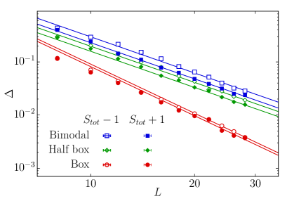
where the couplings are drawn from one of the distributions illustrated in the inset of Fig. 1. The bimodal distribution was studied in Ref. 16. To address possible differences when there is weight at , we also consider the “box” distribution. With periodic boundaries, QMC calculations are affected by the negative sign problem [25] when the number of AF couplings is odd. We therefore impose an even number of instances, which cannot affect the thermodynamic limit.
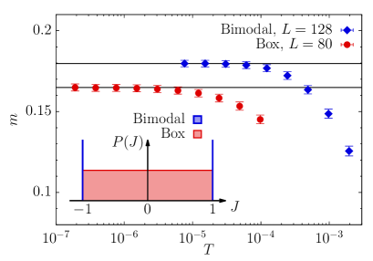
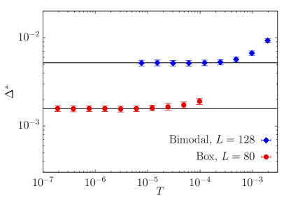
Previous QMC simulations of the model [26, 27] focused on thermodynamic properties at low but nonzero and in general found good agreement with SDRG predictions. While the SSE method also operates at , the ground state can be reached for sufficiently low , as in many previous studies of random quantum spin models [28, 29, 31, 30, 32, 33]. For the F-AF chain we find short autocorrelation and equilibrium times, thus allowing for a large number of disorder samples; here 1000-2000. As shown in Fig. 1, for all practical purposes we reach the ground state for with the bimodal distribution. The convergence is slower for the box distribution, reflecting the fact that it includes , and in this case. We set and use results such as those in Fig. 1 to judge the convergence of all quantities.
An important aspect of the ground state is that it typically has non-zero total spin. For a given sample of the couplings, it is useful to introduce an accumulated phase for each site based on the signs,
| (2) |
so that is classically minimized for . With and denoting the number of and sites, respectively, the ground state has total spin [34], thus is typically of order . It is this growth of with that potentially could enable long-range order, similar to a ferromagnet where , without violating the order-forbidding Mermin-Wagner theorem [35]. We here exclude samples with , so that always holds.
Order parameter.—Working in the basis, it is convenient to define the order parameter in the sector with as [27, 16]
| (3) |
where is the expectation value for an individual sample and denotes sample averaging. Whether or not remains non-zero when is the main point of contention [12, 15, 16]. In our SSE simulations fluctuates among with equal probability, and we group all measurements accordingly. In addition to Eq. (3), we also analyze the longitudinal correlation function
| (4) |
If there is order, then .
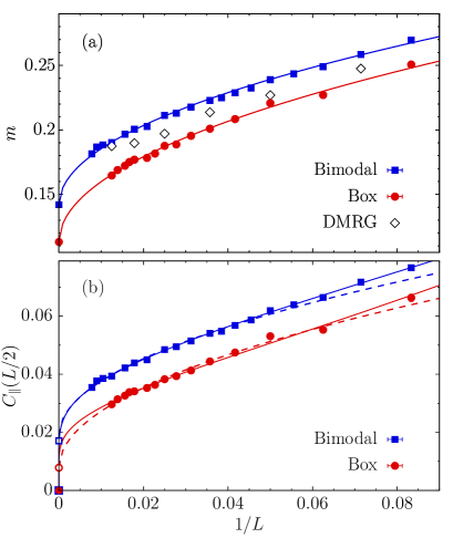
In Fig. 2 we graph both the order parameter and the long-distance correlation function () versus the inverse system size. The results for the two coupling distributions look qualitatively the same. The order parameter can be fitted to the form predicted by SWT, [16], but the long-distance correlation function matches the behavior found within numerical SDRG, [15], which we show in more detail in Appendix A. The correlation function can also be fitted under the assumption of long-range order and is then in reasonable agreement with (slightly below) from Fig. 2(a). From these results alone, neither theory can be ruled out.
In Fig. 2 we also show the DMRG results [16]. Here the data flatten out for the largest systems, seemingly providing a stronger case for an ordered state but conflicting with the SWT predicted correction. The most likely explanation for the observed behavior is that the DMRG results for the largest systems are not fully converged, despite best efforts to control errors. The behavior for the smaller systems is similar to our results, with the overall shift likely a consequence of the different boundary conditions.
Transverse correlations.—The transverse correlation function can be defined in analogy to Eq. (4) using the components of the spins [16]. Here we take a different approach that should be equivalent, using the components but in the sector with :
| (5) |
In the sector the order parameter falls in the -plane, thus for even if the system is ordered. The SWT prediction here is a universal decay, but we are not aware of any SDRG prediction. It should be noted that even if there is no long-range order because .
We only consider the average correlations. The often studied definition of the typical correlation function is slightly biased when the nonlinear operation on the mean correlator of spins , is taken with noisy data before spatial and disorder averaging.
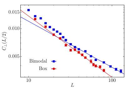
As shown in Appendix B, our results for exhibit a decay with , seemingly in agreement with the SWT prediction (though a logarithmic correction was also predicted for [16]). For the box distribution the decay is faster, with . In both cases, the full behavior versus is much more intricate, however, as shown in Fig. 3(a) and 3(b) for the bimodal and box distribution, respectively. In both cases, the data suggest convergence toward a power law with close to , as shown with fits to a range of for the largest system sizes in each case. Though the exponents may change slightly for larger , it is hard to imagine that the behavior would agree with the SWT form (for the bimodal distribution).
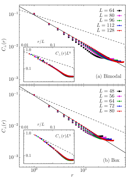
Since and the overall decay applies when , the putative power law can only hold up to ; otherwise a minimum in has to develop, of which we see no sign. In the insets of Fig. 3 we show the correlation functions scaled by and graphed versus . Here we observe data collapse for the larger systems, suggesting that the correlation function is of the form for all , which is still compatible with an independent power law for . In the case of the longitudinal correlations, shown in detail Appendix A, the and behaviors follow the same form.
The transverse correlations were not studied with SDRG and its unusual scaling is another sign of an exotic ground state induced by the random-sign couplings, which force ground states with . If the SWT applies instead, we should have (for the bimodal case, and also more generally for pure dependence) and the collapsed function in Fig. 3(a) would have to change considerably, despite almost absent finite-size corrections with the present system sizes.
The DMRG computed [16] also appears to be described by , and the behavior for small also looks overall similar to our results here, despite the different boundary conditions and slightly different definitions of . It was suggested that the behavior for very large system will eventually agree with the SWT, but there is neither numerical evidence for slow convergence nor predictions of specific large scaling corrections.
Excitation gap.—Next we study the disorder averaged gap , which should depend on the dynamic exponent ; . In the DMRG calculations [16] the gap for a system with spin was computed in the sector. However, the smallest gap is roughly half of the times in the sector, and we here extract the smallest of the two gaps using Lanczos exact diagonalization. In Appendix C, we show that the and gaps scale in the same way, as expected.
In addition to exact disorder averaged gaps for , we also use SSE for an upper bound obtained from well known sum rules [30];
| (6) |
where is the generalized staggered structure factor,
| (7) |
and is the corresponding susceptibility,
| (8) |
Note that, in Eq. (6) the ratio is taken for each coupling realization before disorder averaging. We demonstrate convergence of with lowered in Appendix D.
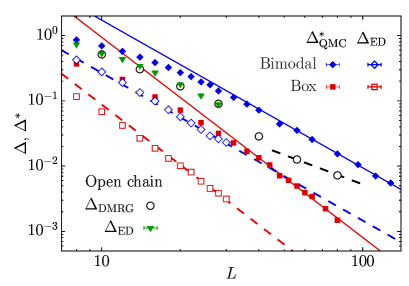
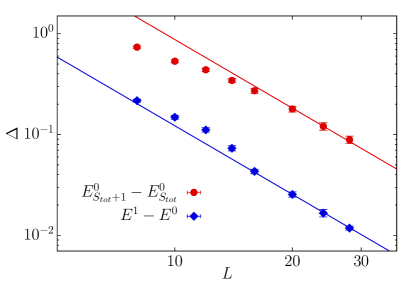
Results for both exact and upper-bound gaps are shown in Fig. 4. Here we indeed observe power law decays, with only small finite-size corrections in the ED data. The upper bounds are much larger than the true gaps, but the scaling is the same for the larger systems. This asymptotic agreement is expected, as the entire low-energy spectrum should exhibit scaling with . We find different dynamic exponents for the two distributions. In the case of the bimodal distribution, the estimate is close to the value obtained with SDRG [13, 14, 10], in that case for several different coupling distributions. There is no visible trend in our data of bringing the exponent to the SWT predicted value eventually. For the box distribution the exponent is larger still, , in apparent conflict with the universal SDRG value.
We also plot the previous DMRG gaps in Fig. 4 and compare with our own ED calculations for open chains. Here we have also used the definition of the gap to the lowest level. The agreement between the DMRG and ED results is good for the systems where both are available. The DMRG results are also largely compatible with our estimate if we assume that the results for the largest systems are affected by minor convergence problems. If we instead take the data at face value as numerically exact, it would appear that the large- behavior agrees with the SWT exponent. However, we find such a rapid change in behavior unlikely.
Discussion.—The non-zero typical spin implies different longitudinal and transverse correlation functions, but this scaling of the spin is not necessarily sufficient for inducing long-range order, unlike the trivial ferromagnet where . However, if there is long-range order, at least some fraction of it must be induced in the spin- components when , as seen in an extreme case of an ground state of a two-dimensional system with an impurity [36].
Given that the longitudinal correlations have the same inverse logarithmic dependence as in the numerical SDRG [15] and that all other results presented here show disagreements with the SWT, the SDRG scenario is most likely qualitatively correct. As a matter of principle, our results still cannot exclude long-range order by some unknown non-SWT mechanism, but we are not aware of any specific proposals for such a scenario.
The differences between the bimodal and box distribution suggest that at least some of the exponents of the fixed point are not universal. We have furthermore demonstrated a unique dual scaling behavior of the transverse correlations that was not predicted by the SDRG. While a power law develops for all , the size dependence remains for even when , in the form . This behavior as well should be a direct consequence of .
Looking back at the DMRG calculations [16], even for is not close to the SWT prediction, while for the short-distance behavior is quite close but only for . Even in the absence of long-range order, for large the SWT predictions should still hold up to some distance, and the behavior for could possibly reflect crossover from the SWT form to a decay to zero in the disordered ground state that we have demonstrated here for . This behavior may possibly persist for all , though a critical above which the system orders cannot be ruled out.
In Appendix C, we also show ED results for the gap scaling in the case of a “half box” coupling distribution , with uniform . The scaling is fully consistent with the same dynamic exponent as with the bimodal distribution, with no apparent differences in the rate of convergence to the asymptotic power law. Based on the results for all three coupling distributions, we therefore conjecture that there are two universality classes of the F-AF chain, for distributions with and without weight at (and possibly other classes for singular distributions). Critical phases with varying exponents have previously been found in two-dimensional quantum spin models, e.g., in Refs. 37, 38, and also there with a competing proposal of ultimately ordered ground state [39]. Further work with different coupling distributions should be carried out to further elucidate the degree of non-universality in the F-AF chain.
Acknowledgements.
Acknowledgments.—We would like to thank Akshat Pandey for discussions prompting us to understake this project and for many valuable comments. This work was supported by the National Natural Science Foundation of China under Grant No. 12122502 and by National Key Projects for Research and Development of China under Grant No. 2021YFA1400400 (H.S.), and by the Simons Foundation under Grant No. 511064 (A.W.S.). Some of the numerical calculations were carried out on the Shared Computing Cluster managed by Boston University’s Research Computing Services.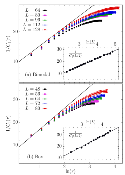
Appendix A Appendix A: Longitudinal correlations
In Fig. 5 we graph the inverse longitudinal correlation function versus for different system sizes, as done for SDRG data in Ref. 15. Though we do not have sufficiently large system sizes to converge to a clear behavior for large , the results are certainly consistent with such behavior with increasing . For the behavior , shown in the insets of Fig. 5, is essentially perfect [as already seen in Fig. 2(b)].
Appendix B Appendix B: Long-distance transverse correlations
Figure 6 shows results for the transverse correlation function at distance . After a cross-over from non-asymptotic behavior, the results for both coupling distributions exhibit good power-law scaling, , with no sign of further significant corrections. The exponent depends on the distribution. A fit to the data for gives for the bimodal distribution, while for the box distribution when fitting to data for .
Interestingly, for the smaller sizes both data sets show the same rate of decay. This behavior can naively be explained by the fact that small systems under the box distribution will only rarely contain couplings very close to , thus the system with bimodal distribution is typically not that different. However, as the system size increases, most samples drawn from the box distribution will have some small couplings, thus the systems can behave differently. This argument does not tell us which one of the system should show a cross-over behavior, which is clearly the bimodal one in Fig. 6. The box distribution gives almost the asymptotic decay already from very small system sizes, while the bimodal system shows a rather sharp crossover around .
In Ref. 16, the SWT predicts for the bimodal distribution, where the multiplicative logarithm would cause an effectively smaller exponent (slower decay) for small , opposite to what we observe in Fig. 6. Thus, we conclude that our results do not support the SWT scenario in this regard. Note that the log correction arises from rare events and was only predicted when , with the pure power law pertaining away from this limit.
Appendix C Appendix C: Gap comparisons
Fava et al. analyzed only the gap between the ground state with spin and the lowest state in the sector [16]. In our ED study we found that the lowest gap has or with the fraction of each approaching with increasing . Though we fully expect the gaps defined in either sector to scale with the same asymptotically, it is still interesting to investigate both definitions. To compare directly with Ref. 16, we first consider open chains and show the results in Fig. 7. Here we indeed find the same scaling for the larger systems, but the mean gap when only using the sector is almost an order of magnitude larger than our definition based on the smallest gap.
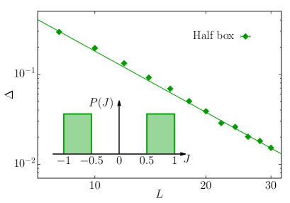
To complement our studies of the bimodal and box coupling distributions, we have also carried out ED calculations of the gap for a “half box” distribution, illustrated in the inset of Fig. 8. Here in the main part of the figure we find that the average gap scales in a way fully consistent with that for the bimodal distribution. Considering also our results for the full box distribution, the good agreement suggests that distributions with weight at behave differently. In principle, if the fixed point from the SDRG calculations applies, one may expect slow convergence to a singular distribution when the microscopic distribution has no weight at . However, since the SDRG procedure for the F-AF chain does not flow to the IRFP, the final distribution should not be extremely singular. Given also the fact that there are no apparent difference in the convergence rate between the full and half box distributions, as shown in Fig. 9 for periodic chains, we find it more likely that distributions with and without weight at fall into (at least) two distinct classes of fixed points.
Appendix D Appendix D: Convergence of the gap bound
In Fig. 1 we demonstrated only the convergence of the order parameter. As another important example, we show in Fig. 10 that the upper bound of the gap Eq. (6) converges even faster.
References
- [1] L. N. Bulaevskii, A. V. Zvarykina, Yu. S. Karimov, R. B. Lyubovskii, and I. F. Shchegolev, Magnetic properties of linear conducting chains, Sov. Phys. JETP 35, 384 (1972).
- [2] G. Theodorou and M. H. Cohen, Paramagnetic Susceptibility of Disordered N-Methyl-Phenazinium Tetracyanoquinodimethanide, Phys. Rev. Lett. 37, 1014 (1976).
- [3] L. J. Azevedo and W. G. Clark, Very-low-temperature specific heat of quinolinium (TCNQ)2, a random-exchange Heisenberg antiferromagnetic chain, Phys. Rev. B 16, 3252 (1977).
- [4] G. Theodorou, Hubbard model for a disordered linear chain: Probability distribution of exchange, Phys. Rev. B 16, 2254 (1977).
- [5] H. M. Bozler, C. M. Gould, and W. G. Clark, Crossover Behavior of a Random-Exchange Heisenberg Antiferromagnetic Chain at Ultralow Temperatures, Phys. Rev. Lett. 45, 1303 (1980).
- [6] L. C. Tippie and W. G. Clark, Low-temperature magnetism of quinolinium (TCNQ)2, a random-exchange Heisenberg antiferromagnetic chain. I. Static properties, Phys. Rev. B 23, 5846 (1981).
- [7] S-k. Ma, C. Dasgupta, and C-k. Hu, Random Antiferromagnetic Chain, Phys. Rev. Lett. 43, 1434 (1979).
- [8] C. Dasgupta, S-k. Ma, Low-temperature properties of the random Heisenberg antiferromagnetic chain, Phys. Rev. Lett. 22, 1305 (1980).
- [9] D. S. Fisher, Random antiferromagnetic quantum spin chains, Phys. Rev. B 50, 3799 (1994).
- [10] F. Iglói and C. Monthus, Strong disorder RG approach of random system, Physics reports 412, 277 (2005).
- [11] F. Iglói and C. Monthus, Strong disorder RG approach - a short review of recent developments, Eur. Phys. J. B 91, 290 (2018).
- [12] A. Furusaki, M. Sigrist, P. A. Lee, K. Tanaka, N. Nagaosa, Random Exchange Heisenberg Chain for Classical and Quantum Spins, Phys. Rev. Lett. 73, 2622 (1994).
- [13] E. Westerberg, A. Furusaki, M. Sigrist, P. A. Lee, Random Quantum Spin Chains: A Real-Space Renormalization Group Study, Phys. Rev. Lett. 75, 4302 (1995).
- [14] E. Westerberg, A. Furusaki, M. Sigrist, P. A. Lee, Low-energy fixed points of random quantum spin chains, Phys. Rev. B 55, 12578 (1997).
- [15] T. Hikihara, A. Furusaki, M. Sigrist, Numerical renormalization-group study of spin correlations in one-dimensional random spin chains, Phys. Rev. B 60, 12116 (1999).
- [16] M. Fava, J. L. Jacobsen, A. Nahum, Heisenberg spin chain with random-sign coupling, arXiv:2312.13452 (2023).
- [17] X. Wan, K. Yang, R. N. Bhatt, Modified spin-wave study of random antiferromagnetic-ferromagnetic spin chains, Phys. Rev. B 66, 014429 (2002).
- [18] T. N. Nguyen, P. A. Lee, H.-C. Zur Loye, Design of a Random Quantum Spin Chain Paramagnet: \ceSr_3CuPt_0.5Ir_0.5O_6, Science 271, 489(1996).
- [19] S. Rapsch, U. Schollwöck, and W. Zwerger, Density matrix renormalization group for disordered bosons in one dimension, Europhys. Lett. 46, 559 (1999).
- [20] A. M. Goldsborough and R. A. Römer, Using entanglement to discern phases in the disordered one-dimensional Bose-Hubbard model, Europhys. Lett. 111, 26004 (2015).
- [21] Y.-P. Lin, Y.-J. Kao, P. Chen, and Y.-C. Lin, Griffiths singularities in the random quantum Ising antiferromagnet: A tree tensor network renormalization group study, Phys. Rev. B 96, 064427 (2017).
- [22] Z.-L. Tsai, P. Chen, Y.-C. Lin, Tensor network renormalization group study of spin-1 random Heisenberg chains, Eur. Phys. J. B 93, 63 (2020).
- [23] A. H. O. Wada and J. A. Hoyos, Adaptive density matrix renormalization group study of the disordered antiferromagnetic spin-1/2 Heisenberg chain, Phys. Rev. B 105, 104205 (2022)
- [24] Y.-T. Lin, S.-F. Liu, P. Chen, and Y.-C. Lin, Random singlets and permutation symmetry in the disordered spin-2 Heisenberg chain: A tensor network renormalization group study, Phys. Rev. Res. 5, 043249 (2023).
- [25] P. Henelius, A. W. Sandvik, Sign problem in Monte Carlo simulations of frustrated quantum spin systems, Phys. Rev. B 62, 1102 (2000).
- [26] B. Frischmuth, M. Sigrist, Low-Temperature Scaling Regime of Random Ferromagnetic-Antiferromagnetic Spin Chains, Phys. Rev. Lett. 79, 147 (1997).
- [27] B. Frischmuth, M. Sigrist, B. Ammon, T. Troyer, Thermodynamics of random ferromagnetic-antiferromagnetic spin- chains, Phys. Rev. B 60, 3388 (1999).
- [28] A. W. Sandvik, Classical percolation transition in the diluted two-dimensional S=1/2 Heisenberg antiferromagnet, Phys. Rev. B 66, 024418 (2002).
- [29] Crossover effects in the random-exchange spin-1/2 antiferromagnetic chain, N. Laflorencie, H. Rieger, A. W. Sandvik, and P. Henelius, Phys. Rev. B 70, 054430 (2004).
- [30] L. Wang, A. W. Sandvik, Low-Energy Dynamics of the Two-Dimensional Heisenberg Antiferromagnetic on Percolating Cluster, Phys. Rev. Lett. 97, 117204 (2006).
- [31] N. Laflorencie, S. Wessel, A. Läuchli, and H. Rieger, Random-exchange quantum Heisenberg antiferromagnets on a square lattice, Phys. Rev. B 73, 060403(R) (2006)
- [32] Y.-R. Shu, D.-X. Yao, C.-W. Ke, Y.-C. Lin, and A. W. Sandvik, Properties of the random-singlet phase: From the disordered Heisenberg chain to an amorphous valence-bond solid, Phys. Rev. B 94, 174442 (2016).
- [33] L. Dao, H. Shao, and A. W. Sandvik, Multiscale Excitations in the Diluted Two-dimensional S = 1/2 Heisenberg Antiferromagnet, arXiv:2408.06749v1.
- [34] E. Lieb, D. Mattis, Ordering Energy Levels of Interacting Spin Systems, J. Math. Phys. 3 749 (1962).
- [35] N. D. Mermin and H. Wagner, Absence of Ferromagnetism or Antiferromagnetism in One- or Two-Dimensional Isotropic Heisenberg Models, Phys. Rev. Lett. 17, 1133 (1966).
- [36] S. Sanyal, A. Banerjee, K. Damle, and A. W. Sandvik, Antiferromagnetic order in systems with doublet ground states, Phys. Rev. B 86, 064418 (2012).
- [37] L. Liu, H. Shao, Y-C. Lin, W. Guo, A. W. Sandvik, Random-Singlet Phase in Disordered Two-Dimensional Quantum Magnet, Phys. Rev. X 8, 041040 (2018).
- [38] L. Liu, W. Guo, A. W. Sandvik, Quantum-critical scaling properties of the two-dimensional random-singlet state, Phys. Rev. B 102, 054443 (2020).
- [39] I. Kimchi, A. Nahum, T. Senthil, Valence Bonds in Random Quantum Magnets: Theory and Application to \ceYbMgGaO_4, Phys. Rev. X 8, 031028 (2018).