FLoD: Integrating Flexible Level of Detail into 3D Gaussian Splatting for Customizable Rendering

Abstract

3D Gaussian Splatting (3DGS) achieves fast and high-quality renderings by using numerous small Gaussians, which leads to significant memory consumption. This reliance on a large number of Gaussians restricts the application of 3DGS-based models on low-cost devices due to memory limitations. However, simply reducing the number of Gaussians to accommodate devices with less memory capacity leads to inferior quality compared to the quality that can be achieved on high-end hardware. To address this lack of scalability, we propose integrating a Flexible Level of Detail (FLoD) to 3DGS, to allow a scene to be rendered at varying levels of detail according to hardware capabilities. While existing 3DGSs with LoD focus on detailed reconstruction, our method provides reconstructions using a small number of Gaussians for reduced memory requirements, and a larger number of Gaussians for greater detail. Experiments demonstrate our various rendering options with tradeoffs between rendering quality and memory usage, thereby allowing real-time rendering across different memory constraints. Furthermore, we show that our method generalizes to different 3DGS frameworks, indicating its potential for integration into future state-of-the-art developments.

Project page: https://3dgs-flod.github.io/flod.github.io/

1 Introduction

Recent advances in 3D reconstruction have led to significant improvements in the fidelity and rendering speed of novel view synthesis. In particular, 3D Gaussian Splatting (3DGS) (Kerbl et al. 2023) has demonstrated photo-realistic quality at exceptionally fast rendering rates. Despite significant advancements, 3DGS imposes substantial memory demands. As the number of intricate objects in the scene increases, more Gaussians are required for accurate modeling, which results in higher memory usage and lower frame rates. The increase in memory demands requires high-end devices with large GPU memory to render the scene, limiting the flexibility to render on devices with varying memory capacities.

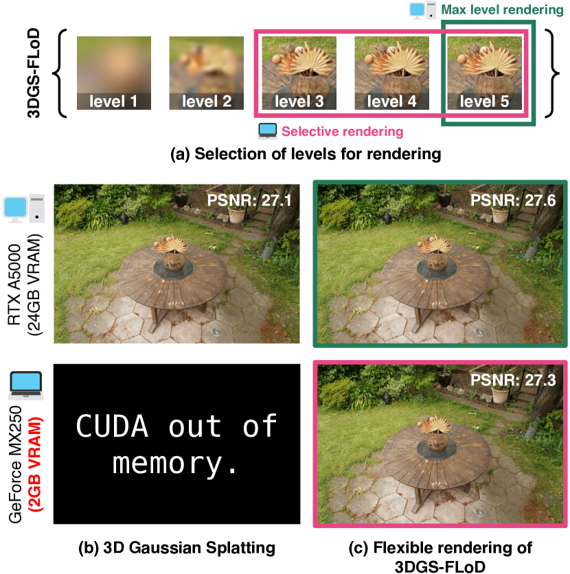
Figure 1: (a) Integration of FLoD into 3DGS enables selection of individual levels or efficient selective rendering with subsets of levels. The green box shows maximum level selection for high-end server, and the pink box shows subset selection for low-cost laptop. (b) 3DGS fails to render on low-cost laptops. (c) Our method supports rendering across diverse hardware settings.

Motivated by the need for greater flexibility in rendering, we integrate the concept of Level of Detail (LoD) within the 3DGS framework. LoD is a concept in graphics and 3D modeling that offers various levels of detail. It enables graphical applications to operate effectively on different systems with varying hardware capabilities by adjusting the level of detail. While recent literature on LoD integration into 3DGS (Ren et al. 2024; Kerbl et al. 2024; Liu et al. 2024) has developed multi-level representations that enable real-time rendering on high-end GPUs with VRAM capacities ranging from 24 to 80GB, these representations lack flexibility for low-cost devices. Therefore, we aim to incorporate LoD into 3DGS to provide more flexible rendering options that can accommodate a wider range of hardware, from high-end servers to everyday laptops.

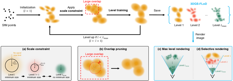
Figure 2: Method overview. Initialized from SfM points, training begins at level 1. (a) Scale constraint is applied to each level. (b) Overlap pruning is performed during level training to mitigate Gaussian overlap. At the end of each level’s training, a clone is saved to compile a multi-level Gaussian set. This level-by-level training process continues until level $L_{\text{max}}$. The resulting multi-level 3DGS, referred to as 3DGS-FLoD, supports (c) maximum level rendering for highest quality or (d) selective rendering using multiple levels for more efficient rendering.

In this paper, we introduce Flexible Level of Detail (FLoD), a method that provides the flexibility to choose levels within 3DGS that meet available memory capacity while preserving the overall scene content. We design each level of Gaussians to have its degree of detail by setting its range of scale. Furthermore, we introduce a level-by-level training method to maintain a consistent 3D structure across levels and to achieve enhanced rendering quality at all levels. Our multi-level representation allows parts of an image to be rendered with different levels of detail, which we refer to as selective rendering. Selective rendering allows for faster and more memory efficient rendering while minimizing the loss in image quality. As a result, FLoD provides users with customizable rendering options that work across devices with different memory capacities.

We empirically validated the effectiveness of FLoD in providing various rendering options. We conducted experiments not only on the Tanks and Temples (Knapitsch et al. 2017) and Mip-Nerf360 (Barron et al. 2022) datasets, which are commonly used in 3DGS and its variants but also on the DL3DV-10K (Ling et al. 2023) dataset, which includes larger and more complex scenes. Through these experiments, we further confirmed that FLoD can be easily integrated into 3DGS-based models and, compared to the base model, enhances rendering quality without additional computational cost.

2 Related Work

2.1 3D Gaussian Splatting

3D Gaussian Splatting (3DGS) (Kerbl et al. 2023) has attained popularity for its fast rendering speed in comparison to other novel view synthesis literature such as NeRF (Mildenhall et al. 2020) and its variants. However, 3DGS has significant runtime memory costs as it typically utilizes a substantial number of Gaussians, making it unsuitable for low-cost devices. Various works on compressing 3DGS propose methods that address these memory issues. For example, LightGaussians (Fan et al. 2023) and Compact3D (Lee et al. 2024) use pruning techniques, while EAGLES (Girish, Gupta, and Shrivastava 2024) employs quantized embeddings. However, their rendering quality falls short compared to 3DGS. RadSplat (Niemeyer et al. 2024) addresses this by leveraging a neural radiance field prior to reduce memory usage while improving rendering quality. Despite this, these methods still do not consider flexibility in rendering memory costs needed to optimize performance across different hardware settings.

In contrast, we propose a multi-level 3DGS that increases rendering flexibility by enabling rendering across a broader range of memory capacities from various hardware configurations, ranging from server GPUs with 24GB VRAM to laptop GPUs with 2GB VRAM.

2.2 Multi-Scale Representation

There have been various attempts to improve rendering quality of novel view synthesis through multi-scale representations. In the field of Neural Radiance Fields (NeRF), approaches such as Mip-NeRF (Barron et al. 2021) and Zip-NeRF (Barron et al. 2023) adopt multi-scale representations to improve rendering fidelity. Similarly, in 3D Gaussian Splatting (3DGS), several methods also incorporate multi-scale representations. For instance, Mip-Splatting (Yu et al. 2024) employs a filtering mechanism, while MS-GS (Yan et al. 2024) creates multiple levels of Gaussians by aggregating small Gaussians from higher levels to handle images with various resolutions. However, these methods primarily focus on addressing the aliasing problem and do not flexibly adapt multiple levels of representation to different device capabilities.

In contrast, our proposed method generates a multi-level representation that not only provides flexible rendering across various hardware settings but also enhances accurate reconstruction.

2.3 Level of Detail

Level of Detail (LoD) in computer graphics uses multiple representations of varying complexity, allowing the selection of detail levels according to computational resources. NGLOD (Takikawa et al. 2021) and Variable Bitrate Neural Fields (Takikawa et al. 2022) create LoD structures based on grid-based NeRFs. In 3D Gaussian Splatting (3DGS), methods such as Octree-GS (Ren et al. 2024) and HierarchicalGaussian (Kerbl et al. 2024) use LoD for efficient rendering by employing lower levels of detail for distant regions and higher levels for areas closer to the viewer. However, these methods focus on rendering with multiple levels simultaneously and lack the ability to render individual levels independently. While CityGaussian (Liu et al. 2024) can render individual levels using its multi-level representations created with various compression rates, it does not address the challenges of rendering on lower-cost hardware.

In contrast, our method allows for the selection of individual or multiple levels for rendering as all levels maintain geometric integrity. Additionally, because each level has appropriate degree of detail and corresponding computational load, our method offers rendering options that can be optimized for various hardware configurations with varying memory capacities.

3 Preliminary

3D Gaussian Splatting (3DGS) (Kerbl et al. 2023) introduces a method to represent a 3D scene using a set of 3D Gaussian primitives. Each 3D Gaussian is characterized by attributes: position $\boldsymbol{\mu}$, opacity $o$, covariance matrix $\boldsymbol{\Sigma}$, and spherical harmonic coefficients. The covariance matrix $\mathbf{\Sigma}$ is factorized into a scaling matrix $\mathbf{S}$ and a rotation matrix $\mathbf{R}$:

$$\boldsymbol{\Sigma}=\mathbf{R}\mathbf{S}\mathbf{S}^{\top}\mathbf{R}^{\top}.$$ (1)

To facilitate the independent optimization of both components, the scaling matrix $\mathbf{S}$ is optimized through the vector $\mathbf{s}_{\text{opt}}$, and the rotation matrix $\mathbf{R}$ is optimized via the quaternion $\mathbf{q}$. These 3D Gaussians are projected to 2D screenspace and the opacity contribution of a Gaussian at a pixel $(x,y)$ is computed as follows:

$$\alpha(x,y)=o\cdot e^{-\frac{1}{2}\left(([x,y]^{T}-\boldsymbol{\mu}^{\prime})^{T}\boldsymbol{\Sigma}^{\prime-1}([x,y]^{T}-\boldsymbol{\mu}^{\prime})\right)},$$ (2)

where $\boldsymbol{\mu}^{\prime}$ and $\boldsymbol{\Sigma}^{\prime}$ are the 2D projected mean and covariance matrix of the 3D Gaussians. The image is rendered by alpha blending the projected Gaussians in depth order.

4 Method: Flexible Level of Detail

Our method reconstructs a scene as a $L_{\text{max}}$-level 3D Gaussian representation, using 3D Gaussians of varying sizes from level 1 to $L_{\text{max}}$ (Section 4.1). Through our level-by-level training process (Section 4.2), each level independently captures the overall scene structure while optimizing for render quality appropriate to its respective level. This process results in a LoD structure of 3D Gaussians, which we refer to as 3DGS-FLoD. The lower levels in 3DGS-FLoD reconstruct the coarse structures of the scene using fewer and larger Gaussians, while higher levels capture fine details using more and smaller Gaussians.while optimizing for render quality appropriate to its respective level. Users can choose any single level from our 3DGS-FLoD for rendering. Additionally, they can collectively use multiple levels to improve rendering efficiency through our selective rendering method (Section 4.4).

4.1 Scale Constraint

For each level $l$ where $l\in[1,L_{\text{max}}]$, we impose a scale constraint $s_{\text{min}}^{(l)}$ as the lower bound on 3D Gaussians. The scale constraint $s_{\text{min}}^{(l)}$ is defined as follows:

$$s_{\text{min}}^{(l)}=\begin{cases}\tau\times\rho^{1-l}&\text{for }1\leq l<L_{\text{max}}\\ 0&\text{for }l=L_{\text{max}}.\end{cases}$$ (3)

$\tau$ is the initial scale constraint and $\rho$ is the scale factor by which the scale constraint is reduced for each subsequent level. The scale constraint is 0 at $L_{\text{max}}$ to allow reconstruction of the finest details without constraints at this stage. Then, we define 3D Gaussians’ scale at level $l$ as follows:

$$\mathbf{s}^{(l)}=e^{\mathbf{s_{\text{opt}}}}+s_{\text{min}}^{(l)}.$$ (4)

where $\mathbf{s_{\text{opt}}}$ is the learnable parameter for scale, while the scale constraint $s_{\text{min}}^{(l)}$ is fixed. We note that $\mathbf{s}^{(l)}>=s_{\text{min}}^{(l)}$ because $e^{\mathbf{s_{\text{opt}}}}>0$.

On the other hand, there is no upper bound on Gaussian size at any level. This allows for flexible modeling, where scene contents with simple shapes and appearances can be modeled with fewer and larger Gaussians, avoiding the redundancy of using many small Gaussians at high levels.

4.2 Level-by-level Training

We design a coarse-to-fine training process, where the next-level Gaussians are initialized by the fully-trained previous-level Gaussians. Similar to 3DGS, the 3D Gaussians at level 1 are initialized from SFM points, and the training for each level involves periodic densification and pruning of Gaussians for a set of iterations. Subsequently, Gaussian attributes are optimized without further densification or pruning for an additional set of iterations. Throughout the entire training process for level $l$, the 3D scale of the Gaussian is constrained to be larger or equal to $s_{\text{min}}^{(l)}$ by definition.

After completing training at level $l$, this stage is saved as a checkpoint. The Gaussians at this point are cloned and saved as the final Gaussians for level $l$. Then the checkpoint Gaussians are used to initialize Gaussians of the next level $l+1$. For initialized Gaussians at the next level $l+1$, we set

$$\mathbf{s}_{\text{opt}}=\textnormal{log}(\mathbf{s}^{(l)}-s_{\text{min}}^{(l+1)}),$$ (5)

such that $\mathbf{s}^{(l+1)}=\mathbf{s}^{(l)}$. It prevents abrupt initial loss by eliminating the gap $\mathbf{s}^{(l+1)}-\mathbf{s}^{(l)}=\cancel{e^{\mathbf{s_{\text{opt}}^{\text{prev}}}}}+s_{\text{min}}^{(l+1)}-(\cancel{e^{\mathbf{s_{\text{opt}}^{\text{prev}}}}}+s_{\text{min}}^{(l)})$.

4.3 Overlap Pruning

We empirically discover that excessive overlap between Gaussians may produce artifacts. To address this, we propose to remove Gaussians with large overlaps, specifically eliminating Gaussians whose average distance of its three nearest neighbors falls below a pre-defined distance threshold $d_{\text{OP}}^{(l)}$. $d_{\text{OP}}^{(l)}$ is set as half of the scale constraint $s_{\text{min}}^{(l)}$ for training level $l$. This method also reduces the overall memory footprint.

4.4 Selective Rendering

Users can get high-quality rendering by using the small and numerous Gaussians at the maximum level. However, such rendering may be slow or even exceed memory limits on commodity devices. Thus, we propose a faster and more memory-efficient rendering method by leveraging our multi-level set of 3D Gaussians $\{\mathbf{G}^{(l)}\mid l=1,\ldots,L_{\text{max}}\}$. Instead of rendering Gaussians from a single level, we assign the Gaussians from multiple levels for different regions of a scene to improve rendering efficiency with minimal quality deficiency.

We create the set of Gaussians $\mathbf{G}_{\text{sel}}$ for selective rendering by sampling Gaussians from a desired level range, $L_{\text{start}}$ to $L_{\text{end}}$:

$$\mathbf{G}_{\text{sel}}=\bigcup_{l=L_{\text{start}}}^{L_{\text{end}}}\left\{G^{(l)}\in\mathbf{G}^{(l)}\mid d_{\text{proj}}^{(l-1)}\geq d_{G^{(l)}}\geq d_{\text{proj}}^{(l)}\right\},$$ (6)

where $d_{\text{proj}}^{(l)}$ decides the inclusion of a Gaussian $G^{(l)}$ whose distance to the camera is $d_{G^{(l)}}$. We define $d_{\text{proj}}^{(l)}$ as:

$$d_{\text{proj}}^{(l)}=\frac{s_{\text{min}}^{(l)}}{\gamma}\times{f},$$ (7)

by solving a proportional equation $s_{\text{min}}^{(l)}:\gamma=d_{\text{proj}}^{(l)}:f$ for the size of a Gaussian on the screensize threshold $\gamma$ and the focal length of the camera $f$. We set $d_{\text{proj}}^{(L_{\text{end}})}=0$ and $d_{\text{proj}}^{(L_{\text{start}}-1)}=\infty$ to ensure that $L_{\text{start}}$ covers the remaining farther regions of the scene not yet covered by the higher levels.

We select Gaussians based on the distance $d_{\text{proj}}^{(l)}$ to reduce computational complexity. This method is feasible because we treat all Gaussians of level $l$ as having a scale equal to $s_{\text{min}}^{(l)}$, during selective rendering, since this represents the smallest scale to which the Gaussians had the freedom to be optimized to. This method is computationally more efficient than the alternative, which would require individually calculating each Gaussian’s 2D projected and comparing it with the screensize threshold $\gamma$ at every level.

The threshold $\gamma$ and the level range [$L_{\text{start}}$, $L_{\text{end}}$] can be adjusted to accommodate specific memory limitations or desired rendering rates. A smaller threshold and a high-level range prioritize fine details over memory and speed, while a larger threshold and a low-level range reduce memory use and speed up rendering at the cost of fine details.

4.5 Compatibility to Different Backbones

Our method’s simplicity in imposing 3D scale constraints on 3D Gaussians makes it easy to integrate with other 3DGS-based techniques. We integrate our approach into Scaffold-GS (Lu et al. 2024), a variant of 3DGS that leverages anchor-based neural Gaussians. We generate a multi-level set of Scaffold-GS by applying progressively decreasing scale constraints on the neural Gaussians, optimized through our level-by-level training method.

	Mip-NeRF360			DL3DV-10K			Tanks&Temples
	$\text{PSNR}\uparrow$	$\text{SSIM}\uparrow$	$\text{LPIPS}\downarrow$	$\text{PSNR}\uparrow$	$\text{SSIM}\uparrow$	$\text{LPIPS}\downarrow$	$\text{PSNR}\uparrow$	$\text{SSIM}\uparrow$	$\text{LPIPS}\downarrow$
3DGS	29.21	0.872	0.140	28.00	0.908	0.142	23.58	0.848	0.177
Scaffold-GS	29.37	0.869	0.147	30.35	0.921	0.123	24.14	0.853	0.174
Octree-GS	29.08	0.867	0.144	30.91	0.931	0.107	24.65	0.865	0.149
3DGS-FLoD	29.65	0.880	0.137	31.75	0.935	0.106	24.33	0.848	0.186

Table 1: Quantitative comparison of 3DGS-FLoD to baselines across three real-world datasets (Mip-NeRF360, DL3DV-10K, Tanks&Temples). The best results are highlighted in bold.

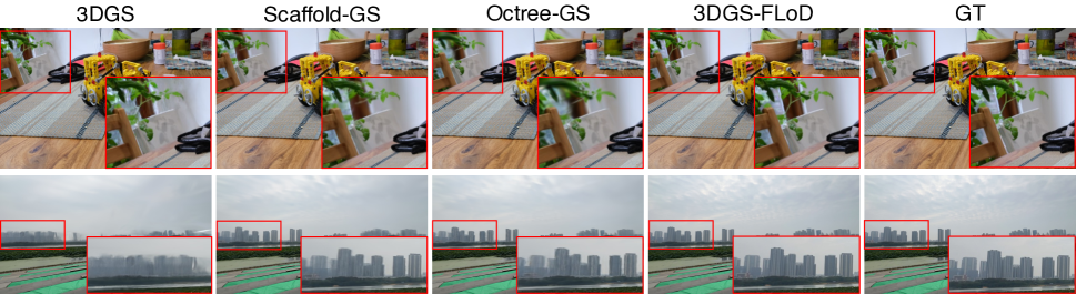
Figure 3: Qualitative comparison between 3DGS-FLoD and baselines on Mip-NeRF360 and DL3DV-10K datasets. The red boxes emphasize the key differences. Please zoom in for a more detailed view.

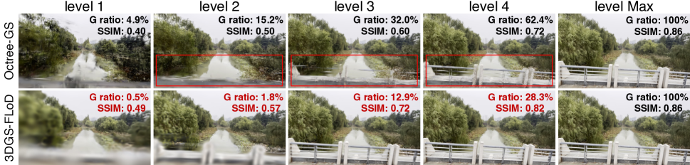
Figure 4: Comparison of single level renderings between Octree-GS and 3DGS-FLoD on the DL3DV-10K dataset. Since Octree-GS has a total of 6 levels and 3DGS-FLoD has 5, we compare the first 4 levels and the maximum level. ”G ratio” refers to the number of Gaussians relative to the maximum level. Red boxes indicate incomplete reconstruction in Octree-GS.

5 Experiment

5.1 Experiment Settings

Datasets

We conducted our experiments on a total of 15 real-world scenes. Two scenes are from Tanks&Temples (Knapitsch et al. 2017) and seven scenes are from Mip-NeRF360 (Barron et al. 2022), encompassing both bounded and unbounded environments. To demonstrate the applicability of our method to more diverse scenes, we also incorporated six unbounded scenes from DL3DV-10K (Ling et al. 2023), which include various urban and natural landscapes. Further details on the datasets can be found in the Appendix.

Evaluation Metrics

We measure PSNR, structural similarity SSIM (Wang et al. 2004), and perceptual similarity LPIPS (Zhang et al. 2018) for a comprehensive evaluation. Additionally, we assess the number of Gaussians used for modeling scenes and the rendering rates (FPS) to evaluate resource efficiency.

Baselines

We compare 3DGS-FLoD against several models, including 3DGS (Kerbl et al. 2023), Scaffold-GS (Lu et al. 2024), and Octree-GS (Ren et al. 2024). Our comparison is restricted to models for which both the paper and code are available. Notably, among 3DGS-based models that handle LoD, only Octree-GS provides publicly available source code . Octree-GS automatically determines the total number of levels based on the scene size, typically generating 6 to 9 levels. While users can manually set the number of levels, performance is generally better with the automatically determined levels. For a fair comparison, we evaluated Octree-GS with its default settings in the subsequent experiments.

Implementation

3DGS-FLoD is implemented on the 3DGS framework. Experiments are mainly conducted on a single NVIDIA RTX A5000 24GB GPU. Following the common practice for LoD in graphics applications, we train our FLoD representation up to level $L_{\text{max}}=5$. $L_{\text{max}}$ is adjustable for specific objectives and settings without significantly affecting render quality. We set the initial scale constraint $\tau=0.2$ and the scale factor $\rho=4$. Densification intervals progressively reduce: 2000, 1000, 500, 500, and 200 for level 1, 2, 3, 4, and 5, respectively. Overlap pruning runs every 1000 iterations for all levels, except the maximum level where it does not run. Following 3DGS, we adopt L1 and SSIM loss for training at all levels. Please check the Appendix for more details on the training setup.

5.2 Results and Evaluation

Quantitative and Qualitative Comparisons

Table 1 quantitatively compare 3DGS-FLoD and the baselines across three real-world datasets. For 3DGS-FLoD, we use the representation at the maximum level (level 5) only, without selective rendering. Notably, 3DGS-FLoD surpasses the baselines in all reconstruction metrics except for the Tanks& Temples dataset, which still shows competitive results. Additionally, as illustrated in Figure 3, 3DGS-FLoD captures thinner structures and represents distant objects more accurately. These advantages stem from our explicit scale constraint for coarse-to-fine training which captures the overall structure at low levels and accurately places high-level Gaussians. Consequently, our approach not only provides LoD but also high-quality rendering.

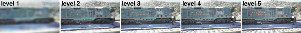
Figure 5: Renderings of each level for FLoD adaptation on Scaffold-GS (Scaffold-GS-FLoD) on the Tanks&Temples dataset.

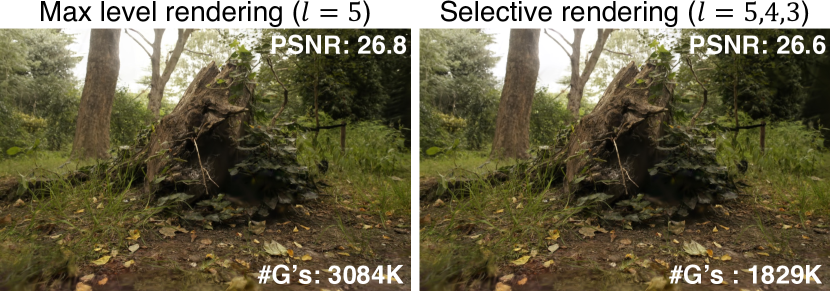
Figure 6: Comparison between level 5 rendering and selective rendering ($l=5,4,3$) on the Mip-NeRF360 dataset. #G’s indicate the total number of Gaussians at the corresponding rendering setting.

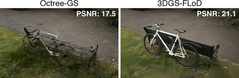
Figure 7: Comparison of renderings with only low-mid levels ($l=3,2,1$) between Octree-GS and 3DGS-FLoD on Mip-NeRF360 dataset.

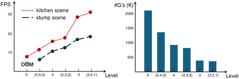
Figure 8: (Left) FPS graph across different levels for two scenes (kitchen and stump) from the Mip-NeRF360 dataset on an MX250 GPU. Curly brackets are used to indicate the level subset for selective rendering. (Right) Average number of Gaussians per level across seven scenes from the Mip-NeRF360 dataset.

LoD Representation Comparison

We compare the properties of each level between our method and Octree-GS in Figure 4. Octree-GS produces broken structures (e.g., bridges) and sharp artifacts (e.g., trees) from level 1 to level 4, while our method preserves the overall structure with appropriate details at each level. The higher SSIM values of our method quantitatively demonstrate its superiority in reconstructing scene structures across these levels. Additionally, our method uses significantly less memory for fewer Gaussians: 0.5%, 1.8%, and 12.9% for levels 1, 2, and 3, respectively, compared to the maximum level. This greater reduction in number of Gaussians enables rendering on devices with lower memory capacities.

Thus, our approach is more suitable for the concept of LoD which offers multiple levels of detail while preserving structure for various memory capacities.

Selective Rendering

Selective rendering assigns a Gaussian level from the chosen range $[L_{\text{start}},L_{\text{end}}]$ based on distance from the camera. It uses lower levels for regions that are farther away. Hence, this approach enables rendering quality of $L_{\text{end}}$ while minimizing memory usage. As shown in Figure 6, selective rendering using levels 3, 4, and 5 achieves visual quality similar to using only level 5 while reducing the number of Gaussians by 40%.

Additionally, we compare selective rendering with levels 1, 2, and 3 as shown in Figure 7. Our method reconstructs the overall geometry of the bench and bicycle while simplifying details in less critical areas, such as grass or asphalt. In contrast, Octree-GS produces fragmented scene reconstruction, with parts of the bicycle and the bench missing.

Furthermore, as shown in Figure 8, selective rendering supports real-time rendering and prevents out-of-memory (OOM) errors on low-cost devices such as the MX250 GPU. This is possible because selective rendering effectively reduces the number of Gaussians used.

Hence, our method offers considerable flexibility by providing various rendering options through selective rendering, ensuring effective performance on devices with varying memory capacities. Refer to the Appendix for more evaluation on the flexibility of selective rendering.

Backbone Compatibility

	$\text{PSNR}\uparrow$	$\text{SSIM}\uparrow$	$\text{LPIPS}\downarrow$	$\text{\#G's}\downarrow$
3DGS	29.21	0.872	0.140	2794K
3DGS-FLoD	29.65	0.880	0.137	2017K
Scaffold-GS	29.37	0.868	0.147	632K
Scaffold-GS-FLoD	29.87	0.873	0.146	607K

Table 2: Quantitative comparison between backbone models and our FLoD adaptation on the Mip-NeRF360 dataset. #G’s indicate the number of Gaussians at the maximum level for our FLoD adpation. For Scaffold-GS and Scaffold-GS-FLoD, the #G’s indicate the number of anchors.

Our method, FLoD, integrates seamlessly with 3DGS and its variants without degradation in image quality. To demonstrate this, we apply FLoD not only to 3DGS (3DGS-FLoD) but also to Scaffold-GS (Scaffold-GS-FLoD). As shown in Table 2, FLoD-integrated models use 4.0% to 27.8% fewer Gaussians compared to the original models while improving image quality. This improvement is likely because large Gaussians at lower levels are fully optimized to represent crucial scene content, since we do not impose an upper bound on the Gaussian scale and use longer densification intervals. As demonstrated in Figure 5, Scaffold-GS-FLoD also effectively generates appropriate representations for each level. Moreover, Scaffold-GS-FLoD also shows an appropriate level of detail on renderings of each level.

Consequently, FLoD can seamlessly integrate into existing 3DGS-based models, providing LoD functionality without degrading rendering quality. Furthermore, we expect FLoD to be compatible with future 3DGS-based models as well.

5.3 Ablation Study

Scale Constraint

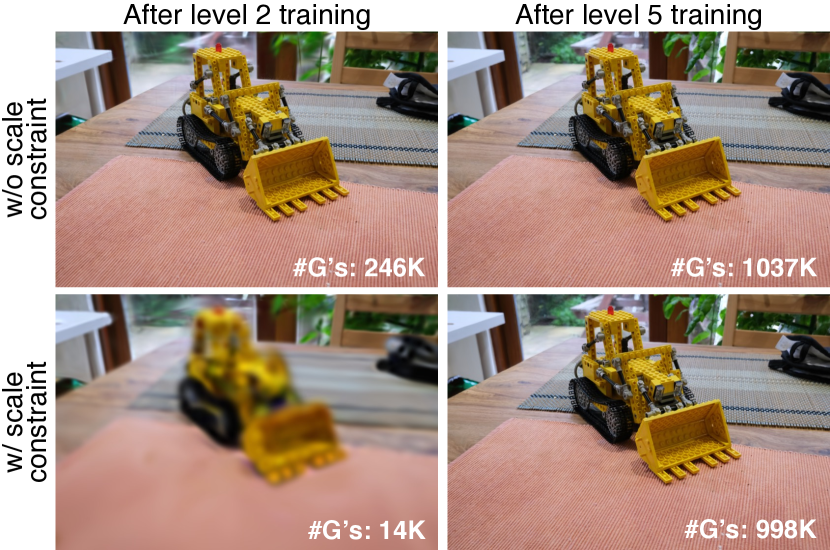
Figure 9: Ablation study of scale constraint on the Mip-NeRF360 dataset.

We compare cases with and without the scale constraint. For the case without the scale constraint, Gaussians are optimized without any size limit. Additionally, we did not apply overlap pruning for this case, as the threshold for overlap pruning $d_{\text{OP}}^{(l)}$ is adjusted proportionally to the scale constraint. Therefore, the case without the scale constraint only applies level-by-level training method from our full method.

As shown in Figure 9, without the scale constraint, the amount of detail reconstructed after level 2 is comparable to that after the maximum level. In contrast, applying the scale constraint results in a clear difference in detail between the two levels. Moreover, the case with the scale constraint uses approximately 98.6% fewer Gaussians compared to the case without the scale constraint. Therefore, the scale constraint is crucial for in ensuring varied detail across levels and enabling each level to maintain a different memory footprint.

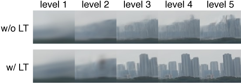
Figure 10: Ablation study of level-by-level training, showing a comparison of rendered images across all levels on the DL3DV-10K dataset. The images are cropped to highlight the most pronounced differences.

Level-by-level Training

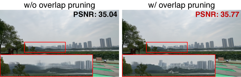
Figure 11: Ablation study of overlap pruning on DL3DV-10K dataset.

We compare cases with and without level-by-level training approach. For the case without level-by-level training approach, the set of iterations for exclusive Gaussian optimization at each level is replaced with iterations that include additional densification and pruning. Figure 10 shows that, without level-by-level training, the reconstructed structure at the intermediate level is inaccurate, leading to a decline in render quality at the higher levels. On the other hand, the case with our level-by-level training better reconstructs scene structure at level 3, increasing reconstruction quality at levels 4 and 5. Hence, level-by level training is important for enhancing reconstruction quality across all levels.

Overlap Pruning

Level	1	2	3	4	5
w/o OP	37K	50K	455K	1013K	2029K
w/ OP	10K	33K	409K	979K	2017K

Table 3: Comparison of the number of Gaussians per level when trained with and without overlap pruning on the Mip-NeRF360 dataset. OP denotes overlap pruning.

We compare the result of training with and without overlap pruning across all levels. As shown in Figure 11, removing overlap pruning deteriorates the structure of the scene, degrading rendering quality. This issue is particularly noticeable in scenes with distant objects. We believe that overlap pruning mitigates the potential for artifacts by preventing the overlap of large Gaussians at distant locations.

Furthermore, we compare the number of Gaussians at each level with and without overlap pruning. Table 3 illustrates that overlap pruning decreases the number of Gaussians, particularly at lower levels, with reductions of 90%, 34%, and 10% at levels 1, 2, and 3, respectively. This reduction is particularly important for minimizing memory usage for rendering on low-cost and low-memory devices that utilize low level representations.

6 Conclusion

In this work, we propose Flexible Level of Detail (FLoD), a method that integrates LoD into 3DGS. FLoD reconstructs the scene in different degrees of detail while maintaining a consistent scene structure. Therefore, our method enables customizable rendering with a subset of levels, allowing the model to operate on devices with various memory capacities, ranging from high-end servers to low-cost laptops. Furthermore, FLoD easily integrates into 3DGS-based models indicating that it will be applicable to upcoming 3DGS-based models as well.

While FLoD-integrated models use less runtime memory than backbone models, they require greater disk storage to accommodate all levels. We believe this limitation can be addressed by incorporating 3DGS compression techniques.

Appendix A Training details

For 3DGS-FLoD training with $L_{\text{max}}=5$ levels, we set the training iterations for levels 1, 2, 3, 4, and 5 to 10,000, 15,000, 20,000, 25,000, and 30,000, respectively. The number of training iterations for the maximum level matches that of the backbone, while the lower levels have fewer iterations due to their faster convergence.

Gaussian density control techniques (densification, pruning, overlap pruning, opacity reset) are performed during the initial 5,000, 6,000, 8,000, 10,000, and 15,000 iterations for levels 1, 2, 3, 4, and 5, respectively. The Gaussian density control techniques run for the same duration as the backbone at the maximum level, but for shorter durations at the lower levels since fewer Gaussians need to be optimized.. Additionally, the intervals for densification are set to 2,000, 1,000, 500, 500, and 200 iterations for levels 1, 2, 3, 4, and 5, respectively. We use longer intervals compared to the backbone, which sets densification and pruning interval to 100, as to allow more time for Gaussians to be optimized before new Gaussians are introduced or existing Gaussians are removed. These settings were selected based on empirical observations.

We set the initial scale constraint $\tau$ to 0.2 with a scale factor $\rho$ of 4. This configuration effectively differentiates the level of detail across $L_{\text{max}}=5$ levels in most tested scenes, allowing for Level of Detail (LoD) representations that adapt to various memory capacities. For smaller scenes or when higher detail is required at lower levels, the scale constraint $\tau$ can be further reduced.

Unlike the original 3DGS approach, we do not periodically remove large Gaussians or those with large projected sizes during training as we do not impose an upper bound on the Gaussian scale. This allows us to model large and simple scene objects with large Gaussians for more efficient scene representation. All other training settings not mentioned follow those of the backbone model.

Appendix B Dataset details

We conduct experiments on the Tanks&Temples dataset  (Knapitsch et al. 2017) and the Mip-NeRF360 dataset (Barron et al. 2022) because they are used for evaluating our baselines: Octree-GS (Ren et al. 2024), 3DGS (Kerbl et al. 2023) and Scaffold-GS (Lu et al. 2024). Additionally, we utilize the recently released DL3DV-10K dataset (Ling et al. 2023) to achieve a more comprehensive evaluation across various scenes. Camera parameters and initial points for all datasets are obtained using COLMAP (Schönberger and Frahm 2016). We subsample every 8th image from each scene for testing, following the train/test splitting methodology presented in Mip-NeRF360.

Tanks&Temples

The Tanks&Temples dataset includes high-resolution multi-view images of various complex scenes, including both indoor and outdoor settings. Following our baselines, we conduct experiments on two unbounded scenes featuring large central objects: train and truck. For both scenes, we reduce the image resolution to $980\times 545$ pixels, downscaling it to 25% of their original size.

Mip-NeRF360

The Mip-NeRF360 dataset (Barron et al. 2022) consists of a diverse set of real-world 360-degree scenes, encompassing both bounded and unbounded environments. The images in the dataset were captured under controlled conditions to minimize lighting variations and avoid transient objects. For our experiments, we use the seven publicly available scenes: bicycle, bonsai, counter, garden, kitchen, room, and stump. We reduce the original image’s width and height to one-fourth. Specifically, the outdoor scenes are resized to approximately $1240\times 830$ pixels, while the indoor scenes are resized to about $790\times 520$ pixels.

DL3DV-10K

The DL3DV-10K dataset (Ling et al. 2023) expands the range of real-world scenes available for 3d representation learning by providing a vast number of indoor and outdoor real-world scenes. For our experiments, we select six outdoor scenes from DL3DV-10K for a more comprehensive evaluation on unbounded real-world environments. We use images with a reduced resolution of $960\times 540$ pixels, following the resolution used in the DL3DV-10K paper. The first 10 characters of the hash codes for our selected scenes are aeb33502d5, 58e78d9c82, df87dfc4c, ce06045bca, 2bfcf4b343, and 9f518d2669.

Level	Training	$\text{PSNR}\uparrow$	$\text{SSIM}\uparrow$	$\text{LPIPS}\downarrow$
5	w/o LT	31.20	0.930	0.158
	w/ LT	31.97	0.936	0.105
4	w/o LT	29.05	0.896	0.161
	w/ LT	30.73	0.917	0.133
3	w/o LT	27.05	0.850	0.224
	w/ LT	28.29	0.869	0.200
2	w/o LT	23.41	0.734	0.376
	w/ LT	24.01	0.750	0.355
1	w/o LT	20.41	0.637	0.485
	w/ LT	20.81	0.646	0.475

Table 1: Quantitative comparison of each level with and without the application of level-by-level training on DL3DV-10K dataset. LT denotes level-by-level training.

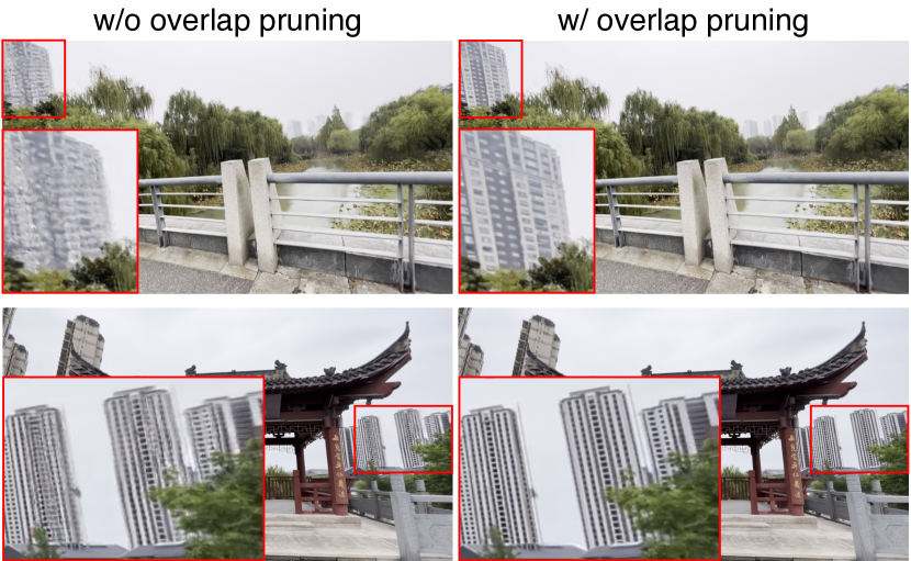
Figure 1: Qualitative comparison of rendering results when trained without and with overlap pruning.

Algorithm 1 Overall Method Algorithm for 3DGS-FLoD

1:  $M\leftarrow\text{SfM Points}$ $\triangleright$ Positions

2:  $S_{\text{opt}},R,C,A\leftarrow\text{InitAttributes}()$ $\triangleright$ Scales, Rotations, Colors, Opacities

3:  for $l=1$ to $L_{\text{max}}$ do

4:     if $l<L_{\text{max}}$ then

5:        $s_{\text{min}}^{(l)}\leftarrow\tau\times\rho^{1-l}$ $\triangleright$ Scale constraint for current level

6:     else

7:        $s_{\text{min}}^{(l)}\leftarrow 0$ $\triangleright$ No constraint at the maximum level

8:     end if

9:     $i\leftarrow 0$ $\triangleright$ Iteration count

10:     while not converged do

11:        $S^{(l)}\leftarrow\text{ApplyScaleConstraint}(S_{\text{opt}},s_{\text{min}}^{(l)})$ $\triangleright$ Each Gaussian’s scale parameter is adjusted as defined in Eq. 4

12:        $I\leftarrow\text{Rasterize}(M,S^{(l)},R,C,A)$

13:        $L\leftarrow\text{Loss}(I,\hat{I})$

14:        $M,S_{\text{opt}},R,C,A\leftarrow\text{Adam}(\nabla L)$ $\triangleright$ Backpropagation

15:        if $i<\text{DensificationIteration}$ then

16:           if $\text{RefinementIteration}(i,l)$ then

17:              $\text{Densification}()$

18:              $\text{Pruning}()$

19:              $\text{OverlapPruning}()$ $\triangleright$ Our overlap pruning

20:           end if

21:        end if

22:        $i\leftarrow i+1$

23:     end while

24:     $\text{SaveClone}(l,M,S^{(l)},R,C,A)$ $\triangleright$ Save clones of level $l$ Gaussians

25:     if $l\neq L_{\text{max}}$ then

26:        $S_{\text{opt}}\leftarrow\text{AdjustScale}(S^{(l)})$ $\triangleright$ Adjust scales for level $l+1$ as defined in Eq. 5

27:     end if

28:  end for

Appendix C Details of Ablation Study

Level-by-level Training

Level-by-level training enhances the accuracy of reconstructed structures across all levels. As demonstrated in Table 1, the case with level-by-level training outperforms the case without it in terms of PSNR, SSIM, and LPIPS at every level.

Overlap Pruning

Overlap pruning plays an important role in controlling the number of Gaussians. Simultaneously, as shown in Figure 1, it helps to reduce artifacts in distant buildings, thereby enhancing render quality.

Appendix D Method Details

D.1 Overall Method Algorithm

The overall process for 3DGS-FLoD is summarized in Algorithm 1

Level
1	2	3	4	5	bicycle	bonsai	counter	garden	room	stump	kitchen
✓					✗	17.36	14.54	✗	13.64	✗	9.46
✓ - ✓ - ✓					5.26	23.57	20.55	6.96	22.62	8.40	15.74
✓ $/\checkmark$					7.97	22.32	20.32	7.31	22.25	10.61	15.56
✓ - ✓ - ✓					8.99	24.68	22.62	8.01	22.87	13.23	16.40
✓					9.29	29.19	27.73	13.68	25.12	17.74	25.73
✓ - ✓ - ✓					9.45	30.16	28.20	14.15	27.55	20.71	26.19

Table 2: Rendering FPS results of 3DGS-FLoD on a laptop with MX250 2GB GPU for 7 scenes from the Mip-NeRF360 dataset. A ”✓” on a single level indicates individual level rendering, while a ”✓” on multiple levels indicates selective rendering. ”✗” represents an OOM error, indicating that rendering FPS could not be measured.

D.2 3D vs 2D Scale Constraint

It is essential to impose the Gaussian scale constraint in 3D rather than on the 2D projected Gaussians. Although applying scale constraints to 2D projections is theoretically possible, it increases geometrical ambiguities in modeling 3D scenes. This is because the scale of the 2D projected Gaussians varies depending on their distance from the camera. Consequently, imposing a constant scale constraint on a 2D projected Gaussian from different camera positions sends inconsistent training signals, leading to Gaussian receiving training signals that misrepresent their true shape and position in 3D space. In contrast, applying the scale constraint to 3D Gaussians ensures consistent enlargement regardless of the camera’s position, thereby enabling stable optimization of the Gaussians’ 3D scale and position.

Level
1	2	3	4	5	PSNR	SSIM	LPIPS	FPS	#G’s
✓					29.65	0.879	0.137	154	2017K
✓- ✓- ✓					28.34	0.855	0.172	206	987K
✓$-\checkmark$					28.57	0.836	0.196	226	979K
✓- ✓- ✓					27.69	0.829	0.203	219	773K
✓					25.47	0.699	0.353	262	409K
✓- ✓- ✓					25.41	0.698	0.354	271	373K

Table 3: Comparison among individual level renderings and selective renderings using different levels in 3DGS-FLoD on the Mip-NeRF360 dataset.

D.3 Selective Rendering

Implementation

When creating the Gaussian subset $\mathbf{G}_{\text{sel}}$ for selective rendering, we calculate the Gaussian distance ($d_{G}$) from the average position of all training view cameras. This is because the average camera position is considered the most representative of the scene. This approach is particularly suitable for the scenes in our experiments, where the camera trajectories either circle around a central object or stay in similar positions while varying the view angle.

Evaluation on Flexibility

Selective rendering enhances efficiency by reducing the number of Gaussians while minimizing the drop in rendering quality as shown in Table 3. For instance, using selective rendering with levels 5, 4, and 3 results in a slight decrease in perceptual metrics compared to using level 5 only, but it reduces the number of Gaussians by 51%, thereby lowering memory usage. This efficiency of selective rendering offers users the flexibility to choose an rendering option with faster rendering speed and reduced memory usage to adapt to different hardware capabilities. As illustrated in Table 2, our FLoD provides rendering options that can avoid out-of-memory (OOM) errors on the low-cost GeForce MX250 2GB GPU, while also enabling real-time rendering in some scenes. This flexibility provides various rendering options suitable for different hardware configurations.

Appendix E Selective Rendering on City-scale Scenes

City-scale scenes, such as Matrix City (Li et al. 2023), consist of environments captured by numerous camera views spread across wide areas. These large scenes are challenging for 3DGS to handle because they require a vast number of Gaussians to represent the scene, leading to high memory usage and necessitating GPUs with large memory capacities. For such extensive scenes, selective rendering is a practical solution to reduce memory usage. By using lower-level Gaussian representations for distant and less important regions, memory requirements can be significantly reduced. This method makes rendering feasible on limited hardware settings.

Moreover, unlike the previously addressed scenes (Mip-NeRF360, DL3DV-10K, Tanks&Temples), city-scale scenes are larger and therefore can require rendering of long camera trajectories. It is essential to dynamically update the subset of Gaussians ($\mathbf{G}_{\text{sel}}$) according to the changes in the camera’s position for consistent rendering quality over long camera trajectories. To achieve this, we introduce multi-threading to periodically update the Gaussian subset ($\mathbf{G}_{\text{sel}}$) in the background during rendering, maintaining rendering quality and enhancing efficiency.

Selective Rendering on Matrix City

We show our selective rendering with periodic updates for a long camera trajectory in the Small City scene from the Matrix City (Li et al. 2023) dataset. We conduct our experiment on a section of the Small City scene, consisting of 320 training images taken along a path long enough to necessitate dynamic Gaussian subset updates.

We conduct the evaluation on both server (NVIDIA RTX 4090 24GB GPU) and laptop (NVIDIA GeForce MX250 2GB GPU) settings to demonstrate that our selective rendering is beneficial across broad range of hardware configurations. We perform Gaussian subset updates every 50 views, as we find this interval sufficient to provide consistent rendering.

As shown in Table 4, applying selective rendering results in a 54 to 130% increase in rendering rates (FPS) compared to using only the maximum level (level 5). However, temporary frame drops occur due to Gaussian subset updates, causing noticeable delays. Our multi-threading approach mitigates these frame drops, accelerating the rendering rate during Gaussian subset updates by 72 to 120%.

This multi-threading approach is particularly important for low-cost laptop settings, as it significantly increases the average rendering rate (FPS), bringing it closer to real-time rendering speeds. Furthermore, Figure 2 illustrates that there is minimal perceptual difference between rendering with only the maximum level and selective rendering. This demonstrates the effectiveness of selective rendering in maintaining image quality while accelerating rendering rates across both hardware settings.

Despite the benefits of multi-threading, our method still experiences delays when updating the Gaussian subsets $\mathbf{G}_{\text{sel}}$. Additionally, similar to 3DGS, training 3DGS-FLoD on the full or larger city-scale scenes results in poor rendering quality or out-of-memory (OOM) errors, as it requires optimizing a vast number of Gaussians at once. We believe that this issue can be addressed by adopting partitioning strategies from VastGaussian (Lin et al. 2024) or HierarchicalGaussian (Kerbl et al. 2024).

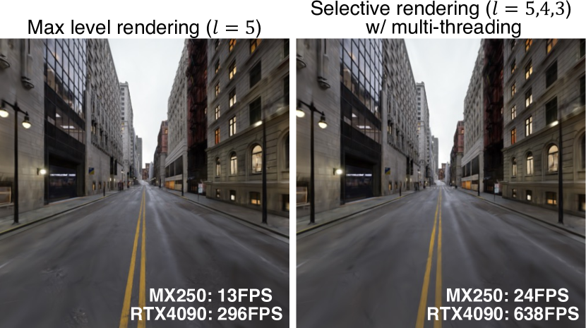
Figure 2: Visual comparison of between maximum level rendering ($l=5$) and selective rendering ($l=5,4,3$) on Matrix City dataset.

	Overall FPS		FPS @ $\mathbf{G}_{\text{sel}}$ update
Rendering Method	Laptop	Server	Laptop	Server
Max level ($l=5$)	13.3	296	-	-
Selective ($l=5,4,3$)	20.5	683	2.91	10.9
+ multi-threading	24.1	637	5.00	24.7

Table 4: FPS comparison between max level rendering and selective rendering in a large scene. For selective rendering, results are also provided with multi-threading. Overall FPS represents the average FPS for rendering all views along the entire camera trajectory. FPS @ $\mathbf{G}_{\text{sel}}$ update indicates the average FPS for every 50th rendering when $\mathbf{G}_{\text{sel}}$ is updated.

Limitation

In scenes with long camera trajectories, frequent Gaussian subset updates can result in frame drops. While implementing multi-threading has partially alleviated this issue, it still persists. Future work could address this by employing an MLP to dynamically generate neural Gaussians of the appropriate level based on the distance from the camera. This approach would reduce the fps drop caused by the Gaussians subset selection process and eliminate the need to store Gaussian representations for all levels.

Appendix F Comparison with Mip-Splatting

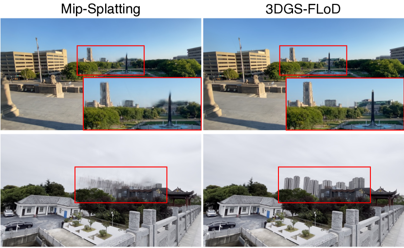
Figure 3: Visual comparison of between 3DGS-FLoD and Mip-Splatting on the DL3DV-10K dataset.

	$\text{PSNR}\uparrow$	$\text{SSIM}\uparrow$	$\text{LPIPS}\downarrow$	$\text{\#G's}\downarrow$
Mip-Splatting	29.51	0.889	0.113	3598K
3DGS-FLoD	29.65	0.880	0.137	2017K

Table 5: Quantitative Comparison between 3DGS-FLoD and Mip-Splatting on the Mip-NeRF360 dataset.

	$\text{PSNR}\uparrow$	$\text{SSIM}\uparrow$	$\text{LPIPS}\downarrow$
Mip-Splatting	28.64	0.917	0.125
3DGS-FLoD	31.97	0.936	0.105

Table 6: Quantitative Comparison between 3DGS-FLoD and Mip-Splatting on the DL3DV-10K dataset.

Mip-Splatting (Yu et al. 2024) is a 3DGS-based model designed for multi-scale rendering. Although Mip-Splatting creates multi-scale representation, it differs from 3DGS-FLoD as Mip-Splatting is designed to address anti-aliasing, not to provide flexible rendering across various hardware settings. Due to the difference in the target tasks, we did not include Mip-Splatting as a baseline in the main paper. However, since both models enhance rendering quality by adjusting the scale of Gaussians, we conducted a comparative performance analysis between Mip-Splatting and 3DGS-FLoD on two datasets: Mip-NeRF360 and DL3DV-10K.

The results on the Mip-NeRF360 dataset (Table 5), which is the primary dataset for Mip-Splatting, show that Mip-Splatting slightly outperforms 3DGS-FLoD in quality metrics other than PSNR. However, it is important to note that 3DGS-FLoD achieves this performance while using approximately 44% fewer Gaussians compared to Mip-Splatting, indicating a more efficient use of resources.

On the DL3DV-10K dataset (Table 6), 3DGS-FLoD significantly outperforms Mip-Splatting. This is particularly evident when comparing the reconstructed results of distant objects, as illustrated in Figure 3. It indicates that the 2D and 3D filtering employed by Mip-Splatting does not improve the reconstruction of large distant objects. In contrast, 3DGS-FLoD is superior in reconstructing distant objects by imposing lower bounds on the Gaussians’ 3D scales.

Appendix G FLoD with LightGS

	FPS	Size(MB)	PSNR	SSIM	LPIPS
3DGS-FLoD	154	477	29.6	0.879	0.127
3DGS-FLoD+LightGS	224	32.2	28.7	0.862	0.165

Table 7: Overall evaluation for level 5 rendering when applying the compression method from LightGaussian (denoted as ’+LightGS’) onto 3DGS-FLoD on the Mip-NeRF360 dataset.

	FPS	Size(MB)	PSNR	SSIM	LPIPS
3DGS-FLoD	14.7	233	28.3	0.855	0.172
3DGS-FLoD +LightGS	23.8	17	27.7	0.833	0.206

Table 8: Overall evaluation for selective rendering with levels 5, 4, and 3 when applying the compression method from LightGaussian onto 3DGS-FLoD with selective rendering on the Mip-NeRF360 dataset.

One of our limitations is that our method occupies a significant amount of storage disk space to accommodate all levels. To address this, we integrate LightGaussian’s (Fan et al. 2023) compression method into 3DGS-FLoD to reduce both storage disk and memory usage. Compressing 3DGS-FLoD reduces 93% of storage disk usage and improves FPS. However this also leads to a decrease in reconstruction quality metrics compared to the original 3DGS-FLoD, as shown in Table 7, but this is similar to how the reconstruction quality of LightGaussian is lower than its baseline model, 3DGS. Likewise, compression is also applicable on our selective rendering as shown in Table 8. Therefore, we demonstrate that 3DGS-FLoD can be further improved to accommodate devices with limited storage capacity as compressing 3DGS-FLoD .

References

- Barron et al. (2021) Barron, J. T.; Mildenhall, B.; Tancik, M.; Hedman, P.; Martin-Brualla, R.; and Srinivasan, P. P. 2021. Mip-NeRF: A Multiscale Representation for Anti-Aliasing Neural Radiance Fields. ICCV.
- Barron et al. (2022) Barron, J. T.; Mildenhall, B.; Verbin, D.; Srinivasan, P. P.; and Hedman, P. 2022. Mip-NeRF 360: Unbounded Anti-Aliased Neural Radiance Fields. CVPR.
- Barron et al. (2023) Barron, J. T.; Mildenhall, B.; Verbin, D.; Srinivasan, P. P.; and Hedman, P. 2023. Zip-NeRF: Anti-Aliased Grid-Based Neural Radiance Fields. ICCV.
- Fan et al. (2023) Fan, Z.; Wang, K.; Wen, K.; Zhu, Z.; Xu, D.; and Wang, Z. 2023. LightGaussian: Unbounded 3D Gaussian Compression with 15x Reduction and 200+ FPS. arXiv:2311.17245.
- Girish, Gupta, and Shrivastava (2024) Girish, S.; Gupta, K.; and Shrivastava, A. 2024. EAGLES: Efficient Accelerated 3D Gaussians with Lightweight EncodingS. arXiv:2312.04564.
- Kerbl et al. (2023) Kerbl, B.; Kopanas, G.; Leimkühler, T.; and Drettakis, G. 2023. 3D Gaussian Splatting for Real-Time Radiance Field Rendering. ACM Transactions on Graphics, 42(4).
- Kerbl et al. (2024) Kerbl, B.; Meuleman, A.; Kopanas, G.; Wimmer, M.; Lanvin, A.; and Drettakis, G. 2024. A Hierarchical 3D Gaussian Representation for Real-Time Rendering of Very Large Datasets. ACM Transactions on Graphics, 43(4).
- Knapitsch et al. (2017) Knapitsch, A.; Park, J.; Zhou, Q.-Y.; and Koltun, V. 2017. Tanks and Temples: Benchmarking Large-Scale Scene Reconstruction. ACM Transactions on Graphics, 36(4).
- Lee et al. (2024) Lee, J. C.; Rho, D.; Sun, X.; Ko, J. H.; and Park, E. 2024. Compact 3D Gaussian Representation for Radiance Field. In Proceedings of the IEEE/CVF Conference on Computer Vision and Pattern Recognition (CVPR).
- Li et al. (2023) Li, Y.; Jiang, L.; Xu, L.; Xiangli, Y.; Wang, Z.; Lin, D.; and Dai, B. 2023. Matrixcity: A large-scale city dataset for city-scale neural rendering and beyond. In Proceedings of the IEEE/CVF International Conference on Computer Vision, 3205–3215.
- Lin et al. (2024) Lin, J.; Li, Z.; Tang, X.; Liu, J.; Liu, S.; Liu, J.; Lu, Y.; Wu, X.; Xu, S.; Yan, Y.; and Yang, W. 2024. VastGaussian: Vast 3D Gaussians for Large Scene Reconstruction. In CVPR.
- Ling et al. (2023) Ling, L.; Sheng, Y.; Tu, Z.; Zhao, W.; Xin, C.; Wan, K.; Yu, L.; Guo, Q.; Yu, Z.; Lu, Y.; Li, X.; Sun, X.; Ashok, R.; Mukherjee, A.; Kang, H.; Kong, X.; Hua, G.; Zhang, T.; Benes, B.; and Bera, A. 2023. DL3DV-10K: A Large-Scale Scene Dataset for Deep Learning-based 3D Vision. arXiv:2312.16256.
- Liu et al. (2024) Liu, Y.; Guan, H.; Luo, C.; Fan, L.; Peng, J.; and Zhang, Z. 2024. CityGaussian: Real-time High-quality Large-Scale Scene Rendering with Gaussians. In ECCV.
- Lu et al. (2024) Lu, T.; Yu, M.; Xu, L.; Xiangli, Y.; Wang, L.; Lin, D.; and Dai, B. 2024. Scaffold-gs: Structured 3d gaussians for view-adaptive rendering. In Proceedings of the IEEE/CVF Conference on Computer Vision and Pattern Recognition, 20654–20664.
- Mildenhall et al. (2020) Mildenhall, B.; Srinivasan, P. P.; Tancik, M.; Barron, J. T.; Ramamoorthi, R.; and Ng, R. 2020. NeRF: Representing Scenes as Neural Radiance Fields for View Synthesis. In ECCV.
- Niemeyer et al. (2024) Niemeyer, M.; Manhardt, F.; Rakotosaona, M.-J.; Oechsle, M.; Duckworth, D.; Gosula, R.; Tateno, K.; Bates, J.; Kaeser, D.; and Tombari, F. 2024. RadSplat: Radiance Field-Informed Gaussian Splatting for Robust Real-Time Rendering with 900+ FPS. arXiv.org.
- Ren et al. (2024) Ren, K.; Jiang, L.; Lu, T.; Yu, M.; Xu, L.; Ni, Z.; and Dai, B. 2024. Octree-GS: Towards Consistent Real-time Rendering with LOD-Structured 3D Gaussians. arXiv:2403.17898.
- Schönberger and Frahm (2016) Schönberger, J. L.; and Frahm, J.-M. 2016. Structure-from-Motion Revisited. In Conference on Computer Vision and Pattern Recognition (CVPR).
- Takikawa et al. (2022) Takikawa, T.; Evans, A.; Tremblay, J.; Müller, T.; McGuire, M.; Jacobson, A.; and Fidler, S. 2022. Variable Bitrate Neural Fields. In ACM SIGGRAPH 2022 Conference Proceedings, SIGGRAPH ’22. New York, NY, USA: Association for Computing Machinery. ISBN 9781450393379.
- Takikawa et al. (2021) Takikawa, T.; Litalien, J.; Yin, K.; Kreis, K.; Loop, C.; Nowrouzezahrai, D.; Jacobson, A.; McGuire, M.; and Fidler, S. 2021. Neural Geometric Level of Detail: Real-time Rendering with Implicit 3D Shapes. In Proceedings of the IEEE/CVF Conference on Computer Vision and Pattern Recognition (CVPR).
- Wang et al. (2004) Wang, Z.; Bovik, A.; Sheikh, H.; and Simoncelli, E. 2004. Image quality assessment: from error visibility to structural similarity. IEEE Transactions on Image Processing, 13(4): 600–612.
- Yan et al. (2024) Yan, Z.; Low, W. F.; Chen, Y.; and Lee, G. H. 2024. Multi-Scale 3D Gaussian Splatting for Anti-Aliased Rendering. In Proceedings of the IEEE/CVF Conference on Computer Vision and Pattern Recognition (CVPR).
- Yu et al. (2024) Yu, Z.; Chen, A.; Huang, B.; Sattler, T.; and Geiger, A. 2024. Mip-Splatting: Alias-free 3D Gaussian Splatting. In Proceedings of the IEEE/CVF Conference on Computer Vision and Pattern Recognition (CVPR), 19447–19456.
- Zhang et al. (2018) Zhang, R.; Isola, P.; Efros, A. A.; Shechtman, E.; and Wang, O. 2018. The Unreasonable Effectiveness of Deep Features as a Perceptual Metric. In CVPR.