Spatio-Temporal Road Traffic Prediction using Real-time Regional Knowledge
Abstract
For traffic prediction in transportation services such as car-sharing and ride-hailing, mid-term road traffic prediction (within a few hours) is considered essential. However, the existing road-level traffic prediction has mainly studied how significantly micro traffic events propagate to the adjacent roads in terms of short-term prediction. On the other hand, recent attempts have been made to incorporate regional knowledge such as POIs, road characteristics, and real-time social events to help traffic prediction. However, these studies lack in understandings of different modalities of road-level and region-level spatio-temporal correlations and how to combine such knowledge. This paper proposes a novel method that embeds real-time region-level knowledge using POIs, satellite images, and real-time LTE access traces via a regional spatio-temporal module that consists of dynamic convolution and temporal attention, and conducts bipartite spatial transform attention to convert into road-level knowledge. Then the model ingests this embedded knowledge into a road-level attention-based prediction model. Experimental results on real-world road traffic prediction show that our model outperforms the baselines.
Introduction
Traffic prediction refers to predicting taffic-related values such as traffic speed or volume (Yuan and Li 2021). From the perspective of urban planning, traffic prediction is essential as it helps to determine traffic signal operation or plan public transportation. From an individual’s point of view, it becomes necessary to plan a trip such as when to leave or which transportation to use given the traffic condition. Traffic prediction is broadly classified into three categories depending on the time period: short-term (a few minutes to an hour), mid-term (within a few hours), and long-term (more than one day) prediction (Hou and Li 2016). A typical application of short-term prediction is a real-time navigation system, and mid/long-term predictions are used for transportation planning.
While most of the previous deep learning approaches have tackled short-term traffic prediction problems (Jiang and Luo 2021), the mid/long-term traffic prediction has recently become increasingly important for advanced traffic management systems (ATMS), especially with the rise of autonomous cars and car-sharing services (Lana et al. 2018; Hoermann, Stumper, and Dietmayer 2017). Unlike short-term prediction, which mainly utilizes graph information of road network, recent studies have shown that mid/long-term traffic prediction benefits from regional knowledge (e.g., Point of Interests (POIs)) (Zhang et al. 2017; Hu et al. 2018; González, Loukaitou-Sideris, and Chapple 2019). However, regional knowledge is not static but dynamic – it may change as a social event occurs or travel demand changes by unexpected causes (Huang et al. 2019). This would be particularly true for those cities with a large population and high density. Thus, existing models that incorporate static regional knowledge for traffic prediction may fail in a complex urban environment where traffic is affected by real-time regional exploitation.
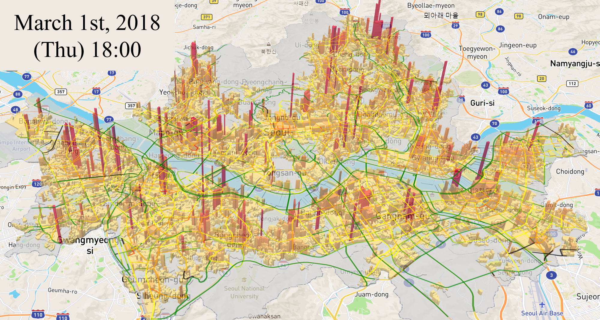
As live regional datasets are becoming more available such as real-time regional population or ridership data as Figure 1, there is increasing interest to utilize this regional knowledge to produce better traffic prediction. In incorporating real-time regional knowledge for traffic prediction, three main challenges remain to be solved as follows:
1) Incorporating region-level and road-level data equally: Previous work (Zhang et al. 2020; Lv et al. 2020; Yuan, Zhou, and Yang 2018) did not handle regional-level and road-level data separately, which may cause performance degradation. For example, it would produce a better result if regional data is analyzed using convolutional neural network (CNN) while road data is incorporated using graph convolutional neural network (GCN).
2) Dynamic regional knowledge learning: Although a model is given real-time regional traffic data and finds certain patterns, it can not solely explain why such patterns occur without background information about the region. The model can have limited learning performance if there is no reasoning from the built-in environment to analyze the regional data. 3) Transformation of regional knowledge into a road: For modality transformation, in determining how much regional information to use for each road, transportation studies typically bound 500m nearby region, which is a walking distance to transit (van Soest, Tight, and Rogers 2020). However, this bound should be adapted differently depending on the road characteristics.
In this study, we propose a novel method to embed both real-time and static regional knowledge for traffic prediction. In particular, we use fine-grained, hourly population estimated from LTE access trace counts together with POIs and satellite images to capture the built-in environment. Our model is composed of a regional spatio-temporal module that consists of dynamic convolution and temporal attention, and conducts bipartite spatial transform attention to convert into road-level knowledge. Then the model ingests this embedded knowledge into a road-level attention-based prediction model. Experimental results show that our model outperforms the baselines. We summarize our contributions as follows:
-
•
To the best of our knowledge, this is the first research that incorporates real-time regional population data for road-level traffic prediction with each modality training. For this, we propose a novel method that learns real-time region-level knowledge for road-level prediction.
-
•
We propose a dynamic convolution based on regional correlation and distance, and a bipartite masked transform attention which adds a gaussian mask to train attention scores from the nearby region for each road.
-
•
We construct real-world dataset in Seoul, Korea, and the evaluation shows that our model outperforms by utilizing real-time regional knowledge. We make our dataset publicly available to contribute research community.
Related Work
Road Traffic Prediction
The biggest challenge of the road traffic prediction model is to use the road connectivity network for training, as the impact of connection in a road graph is higher than the Euclidean distance between traffic sensors. DCRNN (Li et al. 2017) captures spatio information of road graph through diffusion convolution and combines with RNN module to learn spatio-temporal information. ST-MetaNet (Pan et al. 2019) learns the meta knowledge of nodes and edges, and extracts the weights for an RNN cell from meta information to give illusion that each traffic sensor has its own RNN cell that conducts temporal prediction. GMAN (Zheng et al. 2020) leverages spatio-temporal embeddings by Node2Vec (Grover and Leskovec 2016) and timestamps, and applies a spatial attention and a temporal attention combined with a gated fusion. ST-GRAT (Park et al. 2020) proposes sentinel mechanism that complement a spatial attention when there are nodes have less spatial correlation.
Regional Traffic Prediction
For regional traffic prediction models, it is important to learn features for each adjacent cell in a 2D grid. Therefore, a model that passes spatial information through regional filters like convolutional neural network (CNN) and learns temporal information through RNN/temporal attention is mostly proposed. ConvLSTM (Xingjian et al. 2015) is an improved structure that can be used for next video frame prediction by combining a convolution layer instead of fully Connected layer inside LSTM. HeteroConvLSTM (Yuan, Zhou, and Yang 2018) applies this ConvLSTM structure for regional spatio-temporal traffic accident prediction. MC-STGCN (Tang et al. 2021) incorporates spatial correlations among regions using regional community graphs and leverages GRU for temporal correlation learning for better taxi ridership demand prediction.
Multi-modal Traffic Prediction
There are a handful of research that use both real-time region-level and road-level data for prediction. CurbGAN (Zhang et al. 2020) proposes generative adversarial network (GAN) that estimates regional traffic speed from travel demand inferred from taxi ridership. HeteroConvLSTM (Yuan, Zhou, and Yang 2018) transforms the road graph onto 2D-grid region to embed road information for regional traffic prediction. On the other hand, there are several trials to use regional features for traffic prediction. Lv et al. (2020) utilizes POIs with gaussian kernel from each road to capture road-level geographical information to enhance road traffic prediction. Lin et al. (2020) captures land-use proportion within 500m (walking distance) of a subway station for station-level traffic prediction.
Preliminaries
We define our problem as a road traffic prediction using both road and regional traffic history. We denote road traffic data (e.g. traffic speed, traffic flow volume) as , and regional traffic data (e.g. population density, travel demand) as . For a timestamp , , where is the number of grid cells of a -height and -width rectangular region, and where is the number of traffic sensors of the roads. The problem is formulated as finding an optimal function that inputs -temporal history of road and regional traffic data, to output -sequence road traffic prediction of a timestamp , as Equation 1.
| (1) |
Multi-head Attention Mechanism
We leverage dot-product attention (Vaswani et al. 2017) in our method, which has the following form:
| (2) |
with is the attention function, and (query), (key), (value) is formulated by
| (3) |
where , , are inputs for , , and , , are activation functions. In this paper, we denote a non-linear activation function as where , are learnable parameters. is the number of queries and is the number of keys and values. If we use the module as self-attention, and become equal as we input , , the same value. In this work, we employ , , to produce the embedded dimensions of , , to be equally . The attention score calculates values of how will be summed. In multi-headed attention, we concatenate (denoted as ) the output of K-attention heads, and apply an activation . In this study, we set to be for all attention mechanism.
| (4) |
We also denote self attention as for an illustration purpose.
Masked Attention Networks
We leverage masked attention mechanism used in Sperber et al. (2018). The idea is to add mask to attention scores before softmax is applied.
| (5) |
In general, we can apply strict masking to take attention on specific values. We can also apply different masks for multi-head attention heads. We denote multi-head masked attention networks as .
Methodology
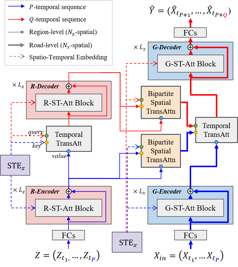
Figure 2 shows overall architecture of our proposed model. Our approach is intuitioned by GMAN (Zheng et al. 2020) that leverages spatio-temporal embeddings for self-attention and transform attention. The biggest difference of our model to GMAN is that we give regional knowledge as query and key to the temporal transform attention of the GMAN block. To begin with, there are spatio-temporal embeddings for road-level () and region-level () which mark the spatial information and timestamps. On the left side, region-level encoder and decoder compute representations of P- and Q-sequence regional data. On the right side, the model leverages the bipartite spatial transform attention to convert this region-level knowledge into road-level knowledge and feed the road-level temporal transform attention. A -stacked ST-Att block simply concatenates a spatio-temporal embedding with the previous hidden output as its input and conducts self-attention, while making the residual addition. A transform attention block (temporal and bipartite spatial) uses different attention query and key depends on how it will transform the input whether in temporal dimension () or in spatial dimension (). In our implementation, all modules produce -dimensional outputs for residual computation.
Spatio-Temporal Embedding
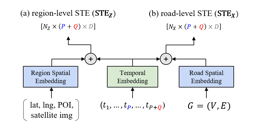
In order to train spatio-temporal knowledge based on the road-network and geographic regional environment, we give different spatio-temporal embeddings (STE) for region-level and road-level. Figure 3 shows how we create spatio-temporal embedding to be used in an attention module.
The STE for regional data () is produced by adding regional spatial embedding with temporal embedding. For a region spatial embedding, we use location (latitude, longitude), POI counts, and satellite image features. We concatenate these geographical features for each cell and apply a 2-layer fully connected network (FCN) to create -dimensional output. For a temporal embedding, we concatenate one-hot encodings of hour-of-day and day-of-week () and apply a 2-layer FCN to create an output. Finally, we add these values in combination of to create .
The STE for road data () is produced as similar to . But, for the road spatial embedding, we use road embedding feature trained from Node2Vec (Grover and Leskovec 2016) using road network, and conduct a 2-layer FCN to create -dimensional output. For the temporal embedding, we share the same one as . Then we add these values in combination of to create .
Spatio Temporal Attention Block
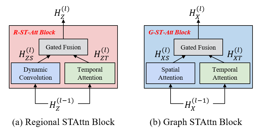
Figure 4 shows the how we implement regional and graph spatio-temporal attention (ST-Att) block. A ST-Att block learns spatio-temporal patterns of the input data by self-attention mechanism. The regional ST-Att (R-ST-Att) block captures spatial pattern by dynamic convolution and temporal pattern by temporal attention. The road graph ST-Att block (G-ST-Att) captures spatial and temporal pattern by respective attention mechanism. In both modules, the gated fusion is applied to sum spatial output and temporal output by trainable ratio that produces optimal output.
Dynamic Convolution
A pair of cell is correlated if their regional characteristics are similar, while there is a less correlation between distant cells. To give regional correlation degraded by distance, we apply a dynamic graph convolution (Zhang et al. 2020) with different edge weights based on Pearson correlation of real-time population on total timespan and distance. We formulate it as with is a row-normalization, is a learnable parameter, and is an edge weight matrix calculated as
| (6) |
where is a pearson correlation between regional traffic data of total timespan, is an Euclidean distance, and is a standard deviation of distances.
Spatial Attention
Basically, a spatial attention and a temporal attention are in the same form, but in different attentional dimension: whether in spatial or temporal. A spatial attention is used for road-level spatial feature extraction by calculating attention score to find correlation between the roads. We first concat to the previous hidden output, and apply a self attention as .
Temporal Attention
The temporal attention is used for both region-level and road-level temporal feature extraction. The module calculates or attention scores depending on the module’s objective is an encoder or decoder. Similar to spatial attention, we first concatenate STE to the input before we apply temporal attention. For each modality, we concatenate corresponding STE with previous hidden output and apply a self attention as , where .
Gated Fusion
In order to mix spatial and temporal hidden outputs depending on their importance, we leverage gated fusion proposed by Zheng et al..
| (7) |
where is an element-wise multiplication and , , are trainable parameters. A gated fusion is used both for R-STAtt and G-STAtt blocks.
Bipartite Spatial Transform Attention
To give real-time regional knowledge for road-level traffic prediction, we propose a bipartite transform attention that converts the spatial modality of regional representations from to . Since a road is affected by its nearby built-in environment (Cervero and Kockelman 1997), we incorporate proximity information on a masked attention network. We give soft gaussian mask intuitioned by Sperber et al. as follows:
| (8) |
Here, is a trainable standard deviation of distances to regional cells from -th road. This enables individual road to train how much proximity information to take. Furthermore, we extend this approach into multi-head masked attention by applying different attention masks for -heads that trains . We formulate this road-level real-time regional knowledge representation as follows:
| (9) |
Temporal Transform Attention
In order to transform the temporal sequence from to for an actual next sequence prediction, we leverage temporal transform attention. As described in Figure 2, we use and temporal sequences of STE or as query and key to calculate attention scores for each modality, and use previous hidden output as value, as follows:
| (10) |
Objective function
We insert 2-layer FCNs at the beginning when we expand dimension from 1 to , and at the end when we shrink to produce the final output from to 1 as described in Figure 2. Using this final output prediction , we train our model using mean absolute error with the ground truth for the objective loss function defined as .
Dataset
Seoul provides road traffic speed111https://topis.seoul.go.kr/refRoom/openRefRoom_1.do and regional living population data222http://data.seoul.go.kr/dataList/OA-14979/F/1/datasetView.do for public data use policy as Figure 1. We construct our real-world urban traffic dataset in three representative downtown regions in Seoul, Korea: Gangnam, Hongik, and Jamsil. The dataset description is listed in Table 1.
Road traffic speed data
Road traffic speed is collected by measuring average hourly traffic speed from GPS signals of around 70,000 taxis in Seoul. We construct a road network using geographic information system (GIS). Each node represents a road while each edge does a link between given two roads. We assume that a traffic sensor is located at the center of a road, and calculate a distance to an adjacent road.
Real-time regional living population (LTE)
We use regional living population estimated hourly from an LTE cell tower. The original data is estimated in zip-code based region unit, but we spatially normalize into 150-meter grid cells. We normalize cell data using training data by the Z-score method, and use this trend data for our model.
| Region | Gangnam | Hongik | Jamsil |
|---|---|---|---|
| #Nodes () | 148 | 93 | 134 |
| #Edges | 1334 | 937 | 1117 |
| Avg. Dist. | 612 | 505 | 530 |
| 34 × 33 | 22 × 27 | 23 × 39 | |
| Avg. #POIs | 79.8 | 55.6 | 32.1 |
| Timespan | 3/1/2018 8/31/2018 (1h, 4392 steps) | ||
Point of Interests (POIs)
We count the number of POIs using the business registration database333https://www.localdata.go.kr/devcenter/dataDown.do. The original data consists of more than 300 subcategories, but we reduce it to 10 representative categories: shopping, food, cafe, beauty, work, hospital, school, art&entertainment, lodging, and nightlife based on Foursquare taxonomy444https://developer.foursquare.com/docs/build-with-foursquare/categories/. Table 2 briefly shows the built-in environment of roads in each region. Gangnam is the most crowded region where every type of POI, including commercial and workplaces, is located. Hongik is less crowded, but still many shops and restaurants are located as well as lodging places for travelers. Jamsil has the least POIs, while a few entertainments such as a stadium and an amusement park are located, although it is not revealed in the table. Many parts of Jamsil consist of residential areas as the high number of schools represents this.
| shop. | work | food | a&e | lodg. | night. | sch. | |
| G | 41.7 | 24.5 | 15.1 | 2.44 | 0.31 | 0.78 | 0.39 |
| H | 27.8 | 21.5 | 20.2 | 1.89 | 1.56 | 0.39 | 0.28 |
| J | 17.3 | 7.1 | 8.2 | 1.91 | 0.33 | 0.48 | 0.45 |
| Model | 1h MAE | 2h MAE | 3h MAE | Avg. MAE | Avg. RMSE | Avg. MAPE | |
|---|---|---|---|---|---|---|---|
| Gangnam | HA | 1.500 | 1.500 | 1.499 | 1.500 | 2.138 | 8.45% |
| SVR/+LTE | 1.505 / 1.436 | 1.835 / 1.688 | 1.959 / 1.780 | 1.766 / 1.635 | 2.467 / 2.279 | 9.91% / 9.14% | |
| RFR/+LTE | 1.328 / 1.406 | 1.522 / 1.588 | 1.593 / 1.663 | 1.481 / 1.552 | 2.045 / 2.148 | 8.20% / 8.55% | |
| DCRNN/+LTE | 1.299 / 1.339 | 1.516 / 1.558 | 1.577 / 1.618 | 1.464 / 1.505 | 1.998 / 2.051 | 7.97% / 8.18% | |
| ST-Meta/+LTE | 1.284 / 1.278 | 1.486 / 1.479 | 1.541 / 1.542 | 1.437 / 1.433 | 1.968 / 1.964 | 7.83% / 7.83% | |
| GMAN/+LTE | 1.319 / 1.314 | 1.407 / 1.402 | 1.444 / 1.438 | 1.390 / 1.385 | 1.904 / 1.897 | 7.56% / 7.57% | |
| OURS | 1.265(.006) | 1.387(.005) | 1.433(.004) | 1.362(.005) | 1.863(.005) | 7.38%(.01%) | |
| Hongik | HA | 1.515 | 1.515 | 1.515 | 1.515 | 2.375 | 7.84% |
| SVR/+LTE | 1.542 / 1.534 | 1.796 / 1.738 | 1.887 / 1.810 | 1.742 / 1.694 | 2.721 / 2.654 | 9.06% / 8.80% | |
| RFR/+LTE | 1.410 / 1.494 | 1.573 / 1.648 | 1.630 / 1.699 | 1.538 / 1.614 | 2.262 / 2.369 | 8.01% / 8.45% | |
| DCRNN/+LTE | 1.373 / 1.379 | 1.516 / 1.531 | 1.559 / 1.573 | 1.482 / 1.494 | 2.227 / 2.262 | 7.67% / 7.72% | |
| ST-Meta/+LTE | 1.386 / 1.380 | 1.543 / 1.535 | 1.593 / 1.579 | 1.507 / 1.498 | 2.282 / 2.258 | 7.77% / 7.74% | |
| GMAN/+LTE | 1.436 / 1.429 | 1.504 / 1.493 | 1.531 / 1.523 | 1.491 / 1.481 | 2.239 / 2.212 | 7.72% / 7.68% | |
| OURS | 1.399(.004) | 1.490(.006) | 1.524(.007) | 1.471(.005) | 2.200(.011) | 7.60%(.06%) | |
| Jamsil | HA | 1.734 | 1.734 | 1.734 | 1.734 | 2.409 | 7.83% |
| SVR/+LTE | 1.657 / 1.675 | 1.941 / 1.907 | 2.060 / 2.014 | 1.886 / 1.866 | 2.658 / 2.599 | 8.34% / 8.30% | |
| RFR/+LTE | 1.536 / 1.612 | 1.728 / 1.820 | 1.806 / 1.913 | 1.690 / 1.782 | 2.360 / 2.489 | 7.46% / 7.85% | |
| DCRNN/+LTE | 1.487 / 1.481 | 1.663 / 1.656 | 1.720 / 1.713 | 1.623 / 1.617 | 2.264 / 2.258 | 7.19% / 7.16% | |
| ST-Meta/+LTE | 1.481 / 1.478 | 1.662 / 1.662 | 1.731 / 1.726 | 1.625 / 1.622 | 2.268 / 2.259 | 7.16% / 7.16% | |
| GMAN/+LTE | 1.574 / 1.580 | 1.674 / 1.673 | 1.726 / 1.720 | 1.658 / 1.658 | 2.306 / 2.302 | 7.31% / 7.31% | |
| OURS | 1.523(.006) | 1.647(.009) | 1.702(.008) | 1.624(.007) | 2.258(.010) | 7.13%(.03%) |
Satellite image features
We extract satellite image features using QGIS VWorld satellite plugin555https://dev.vworld.kr/dev/v4api.do. We combine satellite image patches of cells in three regions, and train a convolutional auto-encoder using 90% of training data and 10% of validation data. Each image patch is resized in size, and we use two stacks of -kernel CNN and CNNtranspose for encoder and decoder. Then we extract the encoded features using its encoder part and reduce the dimension into by principal component analysis.
Experiment
Experimental Settings
Data Processing
We split the dataset successively in 70% of the data for training, 10% of the data for validation, and 20% of the data for testing. We find that the missing values in training data affect the results of all baseline models poorly, so we fill them by next or previous valid values.
Hyperparamters
The model inputs historical time steps (12 hours) to predict the next steps (3 hours) of road traffic values. The hyperparameters for our model are set as , , , , and . The initial learning rate is set to 0.001, and we use Adam optimizer (Kingma and Ba 2014) to train our model. Our model is trained on one GPU environment of NVIDIA GeForce GTX 1080 Ti. We test 5 times and record the average and standard deviation of results.
Metrics
We use three major traffic evaluation metrics: Mean Absolute Error (MAE), Root Mean Squared Error (RMSE), and Mean Absolute Percentage Error (MAPE).
Baselines
We set our baselines as (1) Historical Average based on the hour-of-day and day-of-week (HA), (2) Support Vector Regression (SVR), (3) Random Forest Regression (RFR), (4) DCRNN (Li et al. 2017), (5) ST-MetaNet (Pan et al. 2019), (6) GMAN (Zheng et al. 2020). Unlike GMAN, other models does not have an extra module to embed a temporal timestamp. For SVR and RFR, we give the hour-of-day and the day-of-week of the first timestamp of P input sequences as extra features. For DCRNN, ST-MetaNet, we give these two timestamp information as an additional input, total 3 input channels. For each baseline models, we also test with road-level regional population data by averaging cells within 500 meters (walking distance) from each road, and give as an extra input channel. In this case, the input channel of road traffic data becomes 4 for DCRNN and ST-MetaNet, and 2 for GMAN.
| DCRNN | ST-Meta | GMAN | Ours | |
| # Params | 373,312 | 83,717 | 883,905 | 842,177 |
| Train (s/ep.) | 34.0 | 44.9 | 94.1 | 236.8 |
| # Epochs | 188 | 206 | 36 | 61 |
Experimental results
Forecasting Performance Comparison
Table 3 shows experimental results on our dataset. We denote +LTE as the model with extra LTE input. First of all, our model outperforms the other baselines on average RMSE, and MAPE. Compared to the RNN-based models (DCRNN and ST-MetaNet), the attention based models (GMAN and our model) are better at longer step prediction (2h, 3h). Considering that GMAN is also an attention-based model, the result shows that the improvement of our model is driven by the real-time regional knowledge. In ST-MetaNet and GMAN, the LTE data gives slight more information to improve prediction. However, in DCRNN, it leads to worse prediction in Gangnam and Hongik. Since DCRNN depends more on graph computation, it cannot fully utilize the regional LTE data due to different original modality. On the other hand, ST-MetaNet trains individual parameters for an RNN cell of each traffic sensor and GMAN applies spatial attention, but without an strict attention mask for edge connection, thus they can slightly benefit from LTE data.
Weekly Analysis on Different Road POI Characteristics
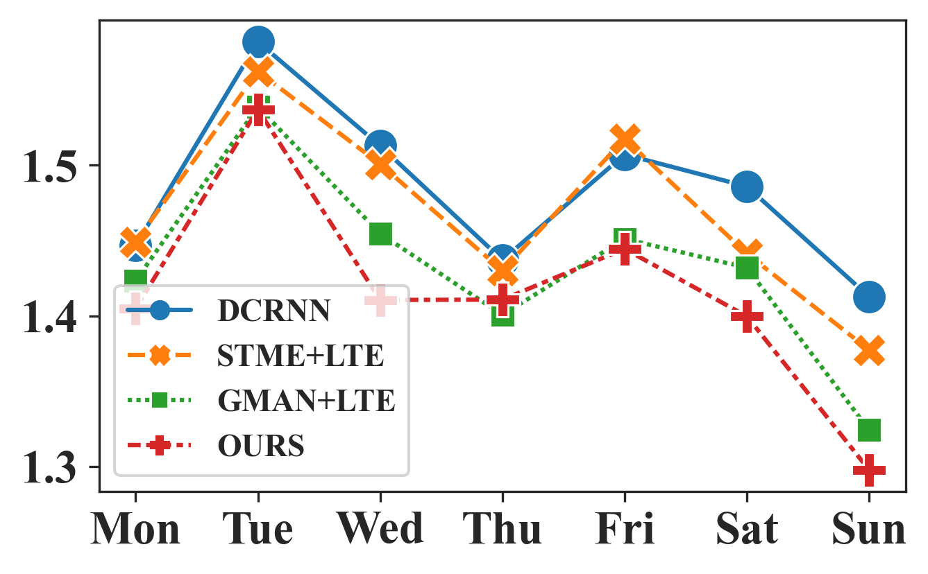
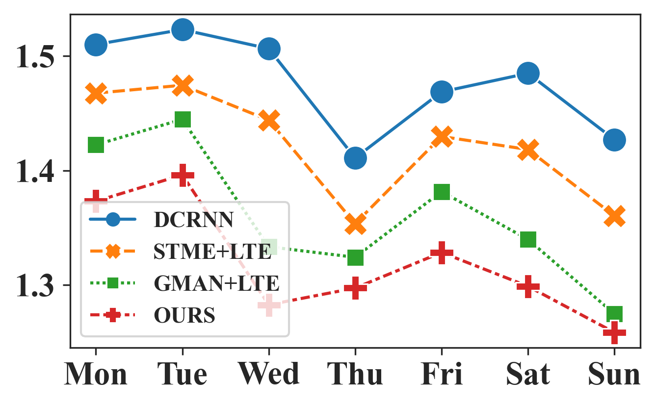
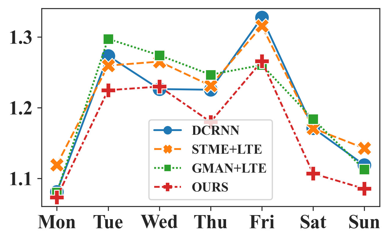
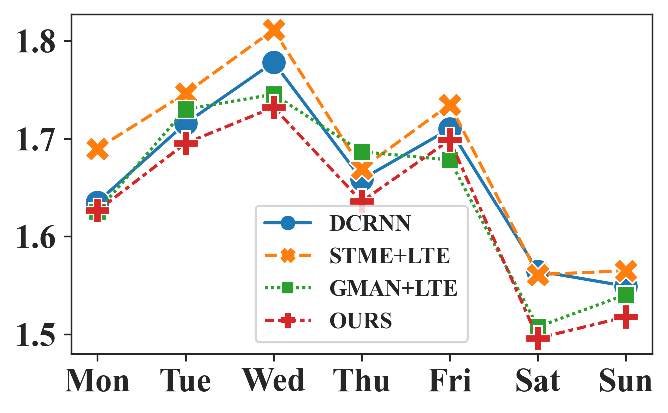
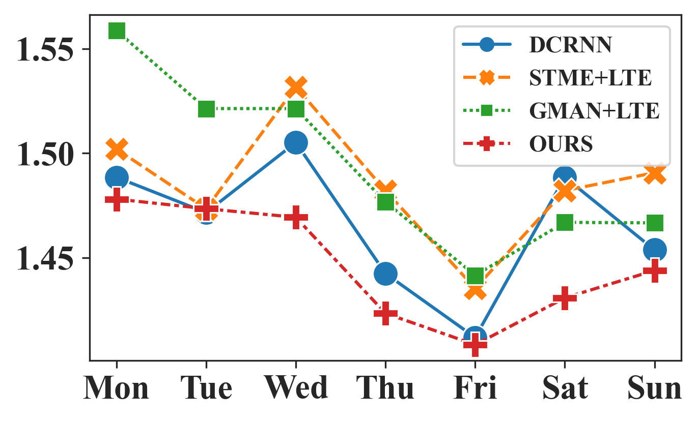
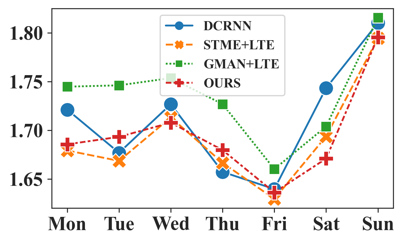
To show how regional knowledge benefits our model, we compare two groups of roads from each region—top 30% of high POI density (POI-H) and bottom 30% of low POI density (POI-L)—and conduct a weekly comparison in Figure 5a. We compare our model with DCRNN, ST-MetaNet+LTE, GMAN+LTE, considering whether they can benefit from LTE data. In general, our model outperforms more in POI-H than in POI-L compare to other baselines. Here, we also measure the weekly maximal performance improvement compare to GMAN+LTE to show how much our model benefits from regional knowledge. In Gangnam, our model is improved up to 3.0% in POI-H and 3.8% in POI-L (Figure 5a (a,b)). When we review Table 2, the POI density is highest in Gangnam among the test regions, so there are still many POIs in POI-L group. This allows our model to perform well on all roads in Gangnam. In Hongik, our model is improved up to 6.5% in POI-H and 3.0% in POI-L (Figure 5a (c,d)). Hongik is visited by people who come for dining and socializing and travelers who come for entertainment. Thus our model primarily benefits on the roads nearby POIs. In Jamsil, our model is improved up to 5.2% in POI-H and 3.4% in POI-L (Figure 5a (e,f)). Since there is a big stadium666https://stadium.seoul.go.kr/board/show-event and an amusement park777https://adventure.lotteworld.com/eng where dynamic social events occur, our model can capture such live regional information to improve our model. On the other hand, the low-POI roads in Hongik and Jamsil are located in residences or freeways, so there is less dynamic regional knowledge that our model can have benefit.
Ablation Study
| # | L. | P. | S. | D. | M. | Gang. | Hong. | Jam. |
|---|---|---|---|---|---|---|---|---|
| a | 0.7 | 1.365 | 1.476 | 1.629 | ||||
| b | 0.5 | 1.366 | 1.472 | 1.635 | ||||
| c | 0.6 | 1.361 | 1.470 | 1.623 | ||||
| d | X | X | 0.6 | 1.549 | 1.582 | 1.729 | ||
| e | X | 0.6 | 1.363 | 1.471 | 1.624 | |||
| f | X | 0.6 | 1.364 | 1.470 | 1.628 | |||
| g | X | X | 1.417 | 1.500 | 1.647 | |||
| h | X | 1.367 | 1.474 | 1.629 | ||||
| i | 0.6 | X | 1.372 | 1.486 | 1.629 |
Table 5 shows effectiveness of each modules of our method. We first empirically measure -value is suitable around 0.6 (#a, #b, #c). When we train our model only with geographic location without POI or satellite image information, the performance gets much worse as LTE data misleads the prediction (#d). However, if we have either POI or satellite image, it gives the POI or land use information that is useful to analyze regional LTE pattern (#e, #f). When we do not consider LTE data, we simply conduct stacks of -kernel 2D-CNN using geographic regional features, and produce static regional knowledge to feed bipartite spatial attention (#g). However, this case does not improve the performance than GMAN since the regional knowledge is not dynamic and limited to provide real-time knowledge. When we replace dynamic convolution into 2D-CNN (#h), the performance gets marginally better than baselines in Table 3, but not the best. When we do not use gaussian mask on bipartite transform attention, the model takes attention even for distant regions of a road, so it lowers performance (#i).
Conclusion
We propose a novel method that learns spatio-temporal regional knowledge via dynamic convolution with temporal attention and transforms it into the road-level feature via the bipartite transform attention to feed a graph multi-attention for the final output. We construct three real-world datasets in Seoul consisting of traffic speed and regional population, and evaluation results show that our model outperforms other baseline models in all regions. Especially, our model performs significantly better on the roads with more POI as more dynamic regional information is available.
We plan to investigate how to enable our model to adaptively learn based on the social sense of place by leveraging temporal POI exploitation and land use. We believe our study provides insights for urban planners and researchers who investigate the correlation between the social use of a region and its corresponding traffic.
References
- Cervero and Kockelman (1997) Cervero, R.; and Kockelman, K. 1997. Travel demand and the 3Ds: Density, diversity, and design. Transportation research part D: Transport and environment, 2(3): 199–219.
- González, Loukaitou-Sideris, and Chapple (2019) González, S. R.; Loukaitou-Sideris, A.; and Chapple, K. 2019. Transit neighborhoods, commercial gentrification, and traffic crashes: Exploring the linkages in Los Angeles and the Bay Area. Journal of Transport Geography, 77: 79–89.
- Grover and Leskovec (2016) Grover, A.; and Leskovec, J. 2016. node2vec: Scalable feature learning for networks. In Proceedings of the 22nd ACM SIGKDD international conference on Knowledge discovery and data mining, 855–864.
- Hoermann, Stumper, and Dietmayer (2017) Hoermann, S.; Stumper, D.; and Dietmayer, K. 2017. Probabilistic long-term prediction for autonomous vehicles. In 2017 IEEE Intelligent Vehicles Symposium (IV), 237–243. IEEE.
- Hou and Li (2016) Hou, Z.; and Li, X. 2016. Repeatability and similarity of freeway traffic flow and long-term prediction under big data. IEEE Transactions on Intelligent Transportation Systems, 17(6): 1786–1796.
- Hu et al. (2018) Hu, W.; Yao, Z.; Yang, S.; Chen, S.; and Jin, P. J. 2018. Discovering urban travel demands through dynamic zone correlation in location-based social networks. In Joint European Conference on Machine Learning and Knowledge Discovery in Databases, 88–104. Springer.
- Huang et al. (2019) Huang, W.; Xu, S.; Yan, Y.; and Zipf, A. 2019. An exploration of the interaction between urban human activities and daily traffic conditions: A case study of Toronto, Canada. Cities, 84: 8–22.
- Jiang and Luo (2021) Jiang, W.; and Luo, J. 2021. Graph neural network for traffic forecasting: A survey. arXiv preprint arXiv:2101.11174.
- Kingma and Ba (2014) Kingma, D. P.; and Ba, J. 2014. Adam: A method for stochastic optimization. arXiv preprint arXiv:1412.6980.
- Lana et al. (2018) Lana, I.; Del Ser, J.; Velez, M.; and Vlahogianni, E. I. 2018. Road traffic forecasting: Recent advances and new challenges. IEEE Intelligent Transportation Systems Magazine, 10(2): 93–109.
- Li et al. (2017) Li, Y.; Yu, R.; Shahabi, C.; and Liu, Y. 2017. Diffusion convolutional recurrent neural network: Data-driven traffic forecasting. arXiv preprint arXiv:1707.01926.
- Lin et al. (2020) Lin, C.; Wang, K.; Wu, D.; and Gong, B. 2020. Passenger flow prediction based on land use around metro stations: a case study. Sustainability, 12(17): 6844.
- Lv et al. (2020) Lv, M.; Hong, Z.; Chen, L.; Chen, T.; Zhu, T.; and Ji, S. 2020. Temporal multi-graph convolutional network for traffic flow prediction. IEEE Transactions on Intelligent Transportation Systems.
- Pan et al. (2019) Pan, Z.; Liang, Y.; Wang, W.; Yu, Y.; Zheng, Y.; and Zhang, J. 2019. Urban traffic prediction from spatio-temporal data using deep meta learning. In Proceedings of the 25th ACM SIGKDD International Conference on Knowledge Discovery & Data Mining, 1720–1730.
- Park et al. (2020) Park, C.; Lee, C.; Bahng, H.; Tae, Y.; Jin, S.; Kim, K.; Ko, S.; and Choo, J. 2020. ST-GRAT: A novel spatio-temporal graph attention networks for accurately forecasting dynamically changing road speed. In Proceedings of the 29th ACM International Conference on Information & Knowledge Management, 1215–1224.
- Sperber et al. (2018) Sperber, M.; Niehues, J.; Neubig, G.; Stüker, S.; and Waibel, A. 2018. Self-attentional acoustic models. arXiv preprint arXiv:1803.09519.
- Tang et al. (2021) Tang, J.; Liang, J.; Liu, F.; Hao, J.; and Wang, Y. 2021. Multi-community passenger demand prediction at region level based on spatio-temporal graph convolutional network. Transportation Research Part C: Emerging Technologies, 124: 102951.
- van Soest, Tight, and Rogers (2020) van Soest, D.; Tight, M. R.; and Rogers, C. D. 2020. Exploring the distances people walk to access public transport. Transport reviews, 40(2): 160–182.
- Vaswani et al. (2017) Vaswani, A.; Shazeer, N.; Parmar, N.; Uszkoreit, J.; Jones, L.; Gomez, A. N.; Kaiser, Ł.; and Polosukhin, I. 2017. Attention is all you need. In Advances in neural information processing systems, 5998–6008.
- Xingjian et al. (2015) Xingjian, S.; Chen, Z.; Wang, H.; Yeung, D.-Y.; Wong, W.-K.; and Woo, W.-c. 2015. Convolutional LSTM network: A machine learning approach for precipitation nowcasting. In Advances in neural information processing systems, 802–810.
- Yuan and Li (2021) Yuan, H.; and Li, G. 2021. A Survey of Traffic Prediction: from Spatio-Temporal Data to Intelligent Transportation. Data Science and Engineering, 6(1): 63–85.
- Yuan, Zhou, and Yang (2018) Yuan, Z.; Zhou, X.; and Yang, T. 2018. Hetero-convlstm: A deep learning approach to traffic accident prediction on heterogeneous spatio-temporal data. In Proceedings of the 24th ACM SIGKDD International Conference on Knowledge Discovery & Data Mining, 984–992.
- Zhang et al. (2017) Zhang, T.; Sun, L.; Yao, L.; and Rong, J. 2017. Impact analysis of land use on traffic congestion using real-time traffic and POI. Journal of Advanced Transportation, 2017.
- Zhang et al. (2020) Zhang, Y.; Li, Y.; Zhou, X.; Kong, X.; and Luo, J. 2020. Curb-GAN: Conditional Urban Traffic Estimation through Spatio-Temporal Generative Adversarial Networks. In Proceedings of the 26th ACM SIGKDD International Conference on Knowledge Discovery & Data Mining, 842–852.
- Zheng et al. (2020) Zheng, C.; Fan, X.; Wang, C.; and Qi, J. 2020. Gman: A graph multi-attention network for traffic prediction. In Proceedings of the AAAI Conference on Artificial Intelligence, volume 34, 1234–1241.