From curve shortening to flat link stability
and Birkhoff sections of geodesic flows
Abstract.
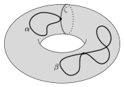
We employ the curve shortening flow to establish three new theorems on the dynamics of geodesic flows of closed Riemannian surfaces. The first one is the stability, under -small perturbations of the Riemannian metric, of certain flat links of closed geodesics. The second one is a forced existence theorem for orientable closed Riemannian surfaces of positive genus, asserting that the existence of a contractible simple closed geodesic forces the existence of infinitely many closed geodesics intersecting in every primitive free homotopy class of loops. The third theorem asserts the existence of Birkhoff sections for the geodesic flow of any closed orientable Riemannian surface of positive genus.
Key words and phrases:
Curve shortening flow, closed geodesics, flat links, Birkhoff sections2020 Mathematics Subject Classification:
53C22, 37D40, 53E10, 53D251. Introduction
On a closed Riemannian surface, the curve shortening flow is the anti-gradient of the length functional on the space of immersed loops. Unlike other more conventional anti-gradient flows on loop spaces, such as the one of the energy functional in the settings [Klingenberg:1978aa], the curve shortening flow is only a semi-flow (i.e. its orbits are only defined in positive time), and the very existence of its trajectories in long time was a remarkable theorem of geometric analysis, first investigated by Gage [Gage:1983aa, Gage:1984aa, Gage:1990aa] and Hamilton [Gage:1986aa], fully settled for embedded loops by Grayson [Grayson:1989aa], and further generalized to immersed loops by Angenent [Angenent:1990aa, Angenent:1991aa]. One of the remarkable properties of the curve shortening flow is that it shrinks loops without increasing the number of their self-intersections. This allowed Grayson to provide a rigorous proof of Lusternik-Schnirelmann’s theorem on the existence of three simple closed geodesics on every Riemannian 2-sphere [Grayson:1989aa, Mazzucchelli:2018aa]. Later on, Angenent [Angenent:2005aa] framed the curve shortening flow in the setting of Morse-Conley theory [Conley:1978aa], and proved a spectacular existence result for closed geodesics of certain prescribed flat-knot types on closed Riemannian surfaces.
The purpose of this article, which is inspired by this latter work of Angenent, is to present new applications of the curve shortening flow to the study of the dynamics of geodesic flows: the stability of certain configurations of closed geodesics under perturbation of the Riemannian metric, the forced existence of closed geodesics intersecting a contractible one, and the existence of Birkhoff sections. We present our main results in detail over the next three subsections.
1.1. -stability of flat links of closed geodesics
The expression of a Riemannian geodesic vector field involves the first derivatives of the Riemannian metric. Therefore, for each integer , a -small perturbation of the Riemannian metric corresponds to a -small perturbation of the geodesic vector field. However, a -small perturbation of the Riemannian metric may result in a drastic deformation of the geodesic vector fields and of its dynamics. For instance, given any smooth embedded circle in a Riemannian surface, one can always find a -small perturbation of the Riemannian metric that makes a closed geodesic for the new metric [Alves:2022aa, Ex. 43]. Moreover, it is always possible to arbitrarily increase the topological entropy of the geodesic flow by means of a -small perturbation of the Riemannian metric [Alves:2022aa, Th. 12].
From the geometric perspective, it is natural to consider the topology on the space of Riemannian metrics: indeed, the length of curves, or more generally the volume of compact submanifolds, vary continuously under -deformations of the Riemannian metric. A result of the first author, Dahinden, Meiwes and Pirnapasov [Alves:2023aa] asserts that the topological entropy of a non-degenerate geodesic flow of a closed Riemannian surface cannot be destroyed by a -small perturbation of the metric. In a nutshell, this can be expressed by saying that the chaos of such geodesic flows is robust. Our first result provides another geometric dynamical property that, unexpectedly, survives after -perturbations of the Riemannian metric of a closed orientable surface: the existence of suitable configurations of closed geodesics. In order to state the result precisely, let us first introduce the setting.
Let be a closed Riemannian surface. We denote by the space of smooth immersions of the circle to , endowed with the topology. The group of smooth diffeomorphisms acts on by reparametrization, and we denote the quotient by . The space consists of unparametrized immersed loops in , and is endowed with the quotient topology. The length functional
is well defined on , meaning that is independent of the specific choice of representative of in , is continuous, and even differentiable for a suitable differentiable structure on . For each integer , we denote by the closed subset of consisting of those multi-loops such that is tangent to for some , or has a self-tangency for some . A path-connected component of is called a flat link type. The reason for this terminology is that lifts into a connected component of the space of links in the projectivized tangent bundle . If , is more specifically called a flat knot type. This terminology was introduced by Arnold in [Arnold:1994aa].
For each integer , we denote by the -fold iterate of a loop . Namely, once we fix a parametrization , we obtain the parametrization , . A loop is primitive if it is not of the form for some and , and otherwise it is an iterated loop. A whole flat knot type is primitive when its closure in contains only primitive loops. Examples of primitive flat knot types include all flat knot types consisting of embedded loops, and all flat knot types consisting of loops whose integral homology class is primitive (i.e. not a multiple , for , of another homology class ). Any flat link type is contained in a product , where the factors are flat knot types, and we say that is primitive when all the factors are primitive flat knot types.
The closed geodesic admits a variational characterization and a dynamical one. The unparametrized closed geodesics of are the critical point of the length functional . The closed geodesics parametrized with unit speed are the base projections of the periodic orbits of the geodesic flow on the unit tangent bundle , ; here, is any geodesic parametrized with unit speed . A closed geodesic of length is non-degenerate when its unit-speed lift is a non-degenerate -periodic orbit of the geodesic flow, meaning that . We introduce the following notion.
Definition 1.1.
A flat link of closed geodesics is stable when every component is non-degenerate and, for each , the components have distinct flat knot types or distinct lengths .
Our first main result is the following.
Theorem A.
Let be a closed Riemannian surface, a primitive flat link type, and a stable flat link of closed geodesics. For each , any Riemannian metric sufficiently -close to has a flat link of closed geodesics such that .
Our inspiration for Theorem A comes from Hofer geometry [Hofer:1990aa, Polterovich:2001aa]. The Hamiltonian diffeomorphisms group of a symplectic manifold admits a remarkable metric, called the Hofer metric, which has a flavor and plays an important role in Hamiltonian dynamics and symplectic topology. When the symplectic manifold is a closed surface, a finite collection of 1-periodic orbits of a non-degenerate Hamiltonian diffeomorphism has a certain braid type . The first author and Meiwes [Alves:2021aa] proved that this property is stable under perturbation that are small with respect to the Hofer metric: any other that is sufficiently close to also has a collection of 1-periodic orbits of braid type . The proof of this result involves Floer theory and holomorphic curves. Later on, employing periodic Floer homology, Hutchings [Hutchings:2023aa] generalized the result to finite collections of periodic orbits of arbitrary period. Our Theorem A can be seen as a Riemannian version of these results. Unlike [Alves:2021aa, Hutchings:2023aa], our proof does not need Floer theory nor holomorphic curves, and instead employs the curve shortening flow.
1.2. Forced existence of closed geodesics
Our next result is an instance of a forcing phenomenon in dynamics: the existence of a particular kind of periodic orbit implies certain unexpected dynamical consequences. For instance, the existence of a hyperbolic periodic point with a transverse homoclinic for a diffeomorphism implies the existence of a horseshoe, which in turn implies the existence of plenty of nearby periodic points and the positivity of topological entropy [Katok:1995aa, Th. 6.5.5]. More in the spirit of our article, Boyland [Boyland:1994aa] proved that the existence of periodic orbits with complicated braid types for a surface diffeomorphism implies complicated dynamical structure, such as the positivity of the topological entropy and the existence of periodic orbits of certain other braid types.
In the specific case of geodesic flows, Denvir and Mackay [Denvir:1998aa] proved that the existence of a contractible closed geodesic on a Riemannian torus, or of three simple closed geodesics bounding disjoint disks on a Riemannian 2-sphere, force the positivity of the topological entropy of the corresponding geodesic flows. A simple argument involving the curve shortening flow further implies the existence of infinitely many closed geodesics in the complement of or of . The forcing theory of Denvir and Mackay was generalized to the category of Reeb flows in [Alves:2022ab, Pirnapasov:2021].
Our second main result is a forced existence theorem for closed geodesics intersecting a simple one, on closed orientable surfaces of positive genus. The statement employs the following standard terminology. A free homotopy class of loops in a surface is a connected component of the free loop space . Notice that this notion is less specific than the one of flat knot type: while every flat knot type corresponds to a unique free homotopy class of loops, a free homotopy class of loops always corresponds to infinitely many flat knot types. A free homotopy class of loops is called primitive when it does not contain iterated loops.
Theorem B.
On any closed orientable Riemannian surface of positive genus with a contractible simple closed geodesic , every primitive free homotopy class of loops contains infinitely many closed geodesics intersecting .
The idea of the proof is to employ a specific Riemannian metric due to Donnay [Donnay:1988ab], which has as closed geodesic. The properties of such a Riemannian metric will allow us to establish the non-vanishing of the local homology of infinitely many “relative” flat-knot types consisting of loops intersecting . Since the local homology of a flat knot type relative to is independent of the choice of the Riemannian metric having as closed geodesic, and its non-vanishing implies the existence of at least a closed geodesic of relative flat knot type , we infer the existence of the infinitely many closed geodesics asserted by Theorem B.
1.3. Existence of Birkhoff sections
While Theorem B has independent interest, our main motivation for it was to combine it with a recent work of the second author together with Contreras, Knieper, and Schulz [Contreras:2022ab] in order to establish a full, unconditional, existence result for Birkhoff sections of geodesic flows of closed surfaces of positive genus. In order to state the result, let us recall the relevant definitions and the state of the art around this problem.
Let be the flow of a nowhere vanishing vector field on a closed 3-manifold . A surface of section is a (possibly disconnected) immersed compact surface whose boundary consist of periodic orbits of , while the interior is embedded in and transverse to . Such a is called a Birkhoff section when there exists such that, for each , the orbit segment intersects . By means of a Birkhoff section, the study of the dynamics of , aside from the finitely many periodic orbits in , can be reduced to the study of the surface diffeomorphism , , where
This reduction is highly desirable, as there are powerful tools that allow to study the dynamics of diffeomorphisms specifically in dimension two (e.g. Poincaré-Birkhoff fixed point theorem, Brower translation theorem, Le Calvez transverse foliation theory, etc.).
The notion of Birkhoff section was first introduced by Poincaré in his study of the circular planar restricted three-body problem, but owes its name to the seminal work of Birkhoff [Birkhoff:1917aa], who established their existence for all geodesic flows of closed orientable surfaces with nowhere vanishing curvature. Over half a century later, a result of Fried [Fried:1983aa] confirmed the existence of Birkhoff sections for all transitive Anosov flows of closed 3-manifolds. In one of the most famous articles from symplectic dynamics [Hofer:1998aa], Hofer, Wysocky, and Zehnder proved that the Reeb flow of any 3-dimensional convex contact sphere admits a Birkhoff section that is an embedded disk. Since this work, the quest for Birkhoff sections of Reeb flows has been a central theme in symplectic dynamics. Recently, the existence of Birkhoff sections for the Reeb vector field of a -generic contact form of any closed 3-manifold has been confirmed independently by the first author and Contreras [Contreras:2022aa], and by Colin, Dehornoy, Hryniewicz, and Rechtman [Colin:2024aa]. Indeed, the existence of Birkhoff sections was proved for non-degenerate contact forms satisfying any of the following assumptions, which hold for a -generic contact form: the transversality of the stable and unstable manifolds of the hyperbolic closed orbits [Contreras:2022aa], or the equidistribution of the closed orbits [Colin:2024aa]. These results extended in different directions previous work of Colin, Dehornoy, and Rechtman [Colin:2023aa], which in particular provided, for any non-degenerate Reeb flows of any closed 3 manifold, a surface of section that is almost a Birkhoff section, except for some escaping half-orbits converging to hyperbolic boundary components of . This result, in turn, relies on Hutchings’ embedded contact homology [Hutchings:2014vp], a powerful machinery based on holomorphic curves and Seiberg-Witten theory, which provides plenty of surfaces of section almost filling the whole ambient 3-manifold. Beyond the above generic conditions, the existence of a Birkhoff section for the Reeb flow of any contact form on any closed 3-manifold remains an open problem.
For the special case of geodesic flows of closed Riemannian surfaces, the non-degeneracy and the transversality of the stable and unstable manifolds of the hyperbolic closed geodesics hold for a generic Riemannian metric, and so does the existence of Birkhoff sections according to the above mentioned result in [Contreras:2022aa]. In a recent work of the first author together with Contreras, Knieper, and Schulz [Contreras:2022ab], this latter result was re-obtained without holomorphic curves techniques, employing instead the curve shortening flow. Actually, the existence result obtained is slightly stronger: the non-degeneracy is only required for the contractible simple closed geodesics without conjugate points. Our third main result removes completely any generic requirement for geodesic flows of closed Riemannian surfaces of positive genus.
Theorem C.
The geodesic flow of any closed orientable Riemannian surface of positive genus admits a Birkhoff section.
The scheme of the proof is the following. Any closed geodesic produces two immersed surfaces of sections of annulus type, the so-called Birkhoff annuli, consisting of all unit tangent vectors based at any point of the closed geodesic and pointing on one of the two sides of it. A surgery procedure due to Fried [Fried:1983aa] allows to glue together all Birkhoff annuli of a suitable collection of non-contractible simple closed geodesics, producing a surface of section . A contractible simple closed geodesic without conjugate points whose unit-speed lifts do not intersect is an obstruction for to be a Birkhoff section. Even after adding to the Birkhoff annuli of , there are still half-orbits of the geodesic flow converging to without intersecting . Theorem B allows us to always detect other closed geodesics intersecting transversely, and after gluing their Birkhoff annuli to we obtain a new surface of section that does not have as -limit of half-orbits not intersecting . As it turns out, after repeating this procedure for finitely many contractible simple closed geodesics without conjugate points, we end up with a Birkhoff section.
1.4. Organization of the paper
In Section 2.1 we recall the needed background on the curve shortening flow, and in particular of Angenent’s version of Morse-Conley theory for it. In Section 3 we prove the simpler, special case of Theorem A for primitive flat knot types, actually under slightly weaker assumptions (Theorem 3.2). In Section 4 we prove a slightly stronger version of Theorem A, replacing the non-degeneracy of the original flat link of closed geodesics with a homological visibility assumption (Theorem 4.7). In Section 5 we prove Theorem B, and in the final Section 6 we prove Theorem C.
1.5. Acknowledgments
The first author thanks Matthias Meiwes and Abror Pirnapasov for many illuminating and inspiring conversations about forcing in dynamics.
2. Preliminaries
2.1. Curve shortening flow
Let be a closed Riemannian surface. The curve shortening flow , for , is a continuous semi-flow on defined as follows: its orbits are solutions of the PDE
for all . Here, is the extended real number giving the maximal interval of definition, is any vector field along that is orthonormal to , and denotes the signed geodesic curvature of with respect to , i.e.
where denotes the Levi-Civita covariant derivative. Notice that we may have if is not orientable, but nevertheless the product is independent of the choice of . We recall that is endowed with the topology, as we specified in the introduction. The map is continuous on its domain of definition, which is an open neighborhood of in . The curve shortening flow is -equivariant, meaning that
and therefore it also induces a continuous semi-flow on the quotient
that we still denote by (we will mainly consider defined on , except if we work with an explicit parametrization of the initial loop ).
The curve shortening flow is the anti-gradient flow of the length functional . More specifically, it satisfies
| (2.1) |
and the equality holds if and only if is a closed geodesic, which is the case if and only if for all .
According to a theorem of Grayson [Grayson:1989aa], if the orbit of an embedded loop is only defined on a bounded interval , then shrinks to a point as ; if instead , then , the curvature converges to zero in the topology as , and in particular there exists a subsequence such that converges to a closed geodesic. This is not necessarily the case if is not embedded, as it may also happen that and develops a singularity as . Nevertheless, the next statement due to Angenent allows to control this behavior.
Let be an immersed loop such that the restriction is an embedded subloop, i.e. and is injective. We say that is a -subloop when it bounds a disk of area less than or equal to , and for some the curves and do not enter (see Figure 1). With the same notation of the introduction, we denote by the closed subspace of consisting of those loops having a self-tangency.

Lemma 2.1 ([Angenent:2005aa], Lemmas 5.3-4)
-
(i)
For each such that as , either converges to a closed geodesic for some sequence , or develops a singularity as . In this latter case, for each and for each sufficiently close to the loop possesses a -subloop.
-
(ii)
There exists with the following property. Let and be such that for all , and assume that is a -subloop for some parametrization on . Then, can be extended to a continuous family of intervals such that is a -subloop for all . ∎
2.2. Primitive flat knot types
Let be either the empty link (when ), or a flat link of pairwise geometrically distinct closed geodesics (namely, and are transverse for all ). We denote by the closed subset of consisting of those loops having a self-tangency or a tangency with some component of (Figure 2). With the notation of Section 1.1, we have
A path-connected component of is called a flat knot type relative (notice that, if is empty, this notion reduces to the one of ordinary flat knot type). We denote by and its closure and its boundary in respectively. The relative flat knot type is called primitive when does not contain non-primitive loops nor components of .
Throughout this section, we work with a primitive flat knot type relative . We recall the main properties of the curve shortening flow with respect to , established by Angenent.
Lemma 2.2 ([Angenent:2005aa], Lemmas 3.3 and 6.2)
-
(i)
If and for some , then for all as well.
-
(ii)
If for some , then for all . ∎
Remark 2.3.
It can be easily shown that the curve shortening flows preserves both the subspace of -th iterates and its complement . This shows that the assumption that is primitive is essential at least for point (ii) of Lemma 2.2.
Lemma 2.4 ([Angenent:2005aa], Lemma 6.3).
The exit set does not depend on the Riemannian metric . ∎
We denote by the open subset of consisting of those containing a -subloop, and we set
| (2.2) |
Lemma 2.5 ([Angenent:2005aa], Prop. 6.8).
The exit-time function
is continuous here, we employ the usual convention . ∎
The continuity of the exit-time function, together with Lemma 2.1(ii), implies that the inclusion is a homotopy equivalence for all . Indeed, its homotopy inverse is given by , where
2.3. Curvature control
In the already mentioned work [Grayson:1989aa], Grayson described the behavior of the curvature of embedded loops that evolve under the curve shortening flow. Actually, the analysis does not require the embeddedness and holds for immersed loops as well, and even in the more general setting of reversible Finsler metrics [De-Philippis:2022aa, Section 2.5]. We summarize here the results needed later on, in Section 4.1, for constructing the suitable neighborhoods of compact sets of closed geodesics that enter the definition of local homology, one of the ingredients of our proof of Theorems A and B.
In order to simplify the notation, for any given immersed loop , we denote by its evolution under the curve shortening flow, and by the signed geodesic curvature of with respect to a normal vector field. In [Gage:1990aa, Lemma 1.2], Gage showed that evolves according to the PDE
| (2.3) |
where denotes the Gaussian curvature of the Riemannian surface along , and is a vector field on , which we see as a differential operator acting on functions , as
We denote by the arclength reparametrization of , where is the function
and by the signed geodesic curvature of .
Proposition 2.6.
For each compact interval there exist such that, for each small enough, for each immersed smooth loop satisfying and , and for each , we have or .
Proof.
We will fix an upper bound for the quantity later on. For now, we consider together with the data stated in the lemma and the notation introduced just before. Notice that and . We denote by the Gaussian curvature of along . We employ (2.3) to compute
If , we can bound from above the term by
We use this inequality as a lower bound for , and continuous the previous estimate as
| (2.4) |
where is a constant depending only on the compact interval and on the Riemannian metric .
We further require , and set
The inequality (2.4) implies
| (2.5) |
Notice that (2.1) can be rewritten in terms of as . This, together with (2.5) and with the initial bound , gives
We claim that, if ,
so that for all . Assume by contradiction that this does not hold, so that . By (2.5) and Gronwall inequality, we have
Therefore , and we infer that . This further implies
By integrating with respect to on , we obtain
which contradicts the fact that .
Next, we compute
and obtain the bound
We denote by a small constant that we will fix later, and set
For each , since
we have . Therefore
| (2.6) |
and, using Peter-Paul inequality,
| (2.7) |
Now, we require and to be small enough (depending only on the compact interval and on the Riemannian metric ) so that, plugging (2.6) and (2.7) into the above estimate of , we obtain
| (2.8) |
3. -stability of closed geodesics within a flat knot type
In this section, we shall prove the much simpler version of Theorem A for the special case of flat links with only one component, that is, flat knots. Actually, the result for flat knots, Theorem 3.2 below, has weaker assumptions: it only requires homotopically visible spectral values, as opposed to homologically visible ones, and does not even need the involved closed geodesics to be isolated.
We employ the notation of Section 2 for a closed Riemannian surface . Let be a primitive flat knot type, and the subset of closed geodesics in . We define the -spectrum
The variational characterization of closed geodesics, together with Sard theorem, implies that is a closed subset of of zero Lebesgue measure. For each subset and , we denote
We define the visible -spectrum to be the set of positive real numbers such that, for any sufficiently small neighborhood of and for some (and thus for all) , the inclusion
is not a homotopy equivalence. It will follow from Lemmas 4.4 and 5.3 that the length of any closed geodesic that is non-degenerate, or more generally homologically visible, belongs to . Conversely, we have the following lemma.
Lemma 3.1.
.
Proof.
Since is a closed subset of , for any we can find such that . We define the continuous function
where is the exit time function of Lemma 2.5. Notice that, actually, is everywhere finite. Indeed, if , then there would exist a sequence with converging to a closed geodesic of length , contradicting the fact that . The map
is a homotopy inverse of the inclusion . ∎
We now prove the anticipated stability of visible spectral values of primitive flat knot types.
Theorem 3.2.
Let be a closed Riemannian surface, a primitive flat knot type, and a visible spectral value. For each , any Riemannian metric sufficiently -close to has a visible spectral value in , i.e.
Proof.
In order to simplify the notation, for each and we denote
Let be small enough so that, for any neighborhood of and for any , the inclusion is not a homotopy equivalence. Since the -spectrum is closed and has measure zero, there exist values
such that
We fix close enough to so that and for all , and . Let be a Riemannian metric on such that
| (3.1) |
where and are the Riemannian densities on associated with and respectively. For each and we denote
Notice that, by (3.1), we have
We fix such that for all . We obtain a diagram of inclusions
Since , , and are homotopy equivalences, whereas is not a homotopy equivalence, we infer that is not a homotopy equivalence neither, and therefore
4. -stability of flat links of closed geodesics
4.1. Neighborhoods of compact subsets of closed geodesics
Let be a closed oriented surface, and a flat knot type. We recall that, for each , the curve shortening flow trajectory is defined on the maximal interval . We set
so that is the maximal interval such that the trajectory stays in the flat knot type . For each subset , we denote its flowout in under the curve shortening flow by
The following statement provides suitable neighborhoods of the compact sets of closed geodesic of a given length. We recall that is endowed with the quotient -topology. Since we will also consider subsets that are open in the coarser topology, we will always specify whether a subset is -open or -open.
Lemma 4.1.
For each compact interval and for each -open neighborhood of there exist and a -open neighborhood of such that, whenever and for some , we have .
Proof.
For each , we denote by the signed geodesic curvature of its arclength parametrization with respect to a normal vector field, as in Section 2.3. The family of subsets
is a fundamental system of -open neighborhoods of the compact set of closed geodesics . For each , the subset
is a -open neighborhood of . Therefore, the statement is a direct consequence of Proposition 2.6. ∎
Let, , and be a connected component of the compact subset of closed geodesics . We define a Gromoll-Meyer neighborhood of to be a (not necessarily open) neighborhood of such that and for some . The reason for this terminology is due to an analogy with the neighborhoods introduced in the seminal work of Gromoll and Meyer [Gromoll:1969aa, Gromoll:1969ab]. While in standard Morse theoretic settings one can always construct arbitrarily small open Gromoll-Meyer neighborhoods, in our setting of the curve shortening flow we can only insure the existence of arbitrarily -small Gromoll-Meyer neighborhoods, essentially as a consequence of Lemma 4.1. We stress that Gromoll-Meyer neighborhoods are not -open, but of course they must contain a -open neighborhood of .
Lemma 4.2.
Any connected component of admits an arbitrarily -small Gromoll-Meyer neighborhood.
Proof.
Let be a connected component of , and the union of the remaining connected components. We consider two arbitrarily small disjoint -open neighborhoods and of and respectively. By Lemma 4.1, there exists , a -open neighborhood of , and a -open neighborhood of such that, whenever and for some , we have . The intersection
is a Gromoll-Meyer neighborhood of contained in . ∎
4.2. Homologically visible closed geodesics
A closed geodesic is called isolated when it is an isolated point of , where is its flat knot type. The local homology of , in the sense of Morse theory, is the relative homology group with integer coefficients
where , is a Gromoll-Meyer neighborhood of such that , and is small enough. By a simple deformation argument employing the curve shortening flow and Lemma 4.1, one readily sees that is independent of the choice of and (we stress that this is the case also for ). Moreover, depends only on the Riemannian metric in a neighborhood of . More precisely, for any -open neighborhood of , we can choose the Gromoll-Meyer neighborhood to be contained in , and by the excision property of singular homology the inclusion induces an isomorphism
The closed geodesic is called homologically visible when it is isolated and has non-trivial local homology.
In the literature, usually the local homology of an isolated closed geodesic is defined in the setting of the free loop space , or equivalently in suitable finite dimensional subspaces of piecewise broken geodesic loops. Let us briefly recall the construction, and refer the reader to, e.g., [Rademacher:1992aa, Bangert:2010aa, Asselle:2018aa] for more details. The energy functional is defined by
We fix a small open geodesic segment intersecting an isolated closed geodesic orthogonally at a single point. For a positive integer , we introduce the space
Here, denotes the Riemannian distance, and the injectivity radius. We see as a subspace of consisting of broken geodesic loops: namely, each corresponds to the piecewise smooth loop such that each restriction is the shortest geodesic segment joining and . The restricted energy functional is given by
We require to be large enough so that our original closed geodesic is of the form for some . Since is an isolated closed geodesic, the corresponding is an isolated critical point of (see [Asselle:2018aa, Prop. 3.1]). We equip with the Riemannian metric , and denote by the flow of the anti-gradient . We denote the flowout of a subset by
Moreover, we denote
Let . In the setting of broken geodesic loops, a Gromoll-Meyer neighborhood is a neighborhood of such that and for some . The relative homology group
is the local homology of the closed geodesic in the setting . Since is an isolated critical point of the smooth function , is finitely generated, see [Gromoll:1969aa, page 364]. We employ the local homology in the finite dimensional setting of broken geodesic loops in order to prove the following two lemmas.
Lemma 4.3.
For any isolated closed geodesic , the local homology is isomorphic to a subgroup of . In particular, is finitely generated.
Proof.
From now on, for each sufficiently -close to , we fix the unique parametrization such that is the intersection point , the speed is constant, and points to the same side of as . We fix a Gromoll-Meyer neighborhood of such that , and a -open neighborhood of that is small enough so that we have a well defined continuous map
Notice that .
We fix a -open neighborhood of the compact set of closed geodesics , where . We fix a Gromoll-Meyer neighborhood of , and a subset that is the union of Gromoll-Meyer neighborhoods of the connected components of . We fix small enough as in the definition of local homology, and such that
We replace , , and with , , and respectively, so that in particular
We set . We also fix , and consider the subspace introduced in (2.2). By excision, the inclusion induces a homology isomorphism
Moreover, the inclusion
is a homotopy equivalence, whose homotopy inverse can be built by pushing with the curve shortening flow. Overall, we infer that the inclusion induces a homology isomorphism
Since is disjoint union of and , we have
and therefore we infer that the inclusion induces an injective homomorphism
Since is a Gromoll-Meyer neighborhood of the isolated closed geodesic , the inclusion induces an isomorphism
and therefore an injective homomorphism
We embed into an Euclidean space , and consider a tubular neighborhood of with associated smooth projection . We consider a sequence of smooth functions , for , that converge to the Dirac delta at the origin as . For each small enough, we have a continuous map
where is the constant speed reparametrization of the loop . Notice that
Since converges to the Dirac delta at the origin as , for all small enough we have
In particular and . The composition restricts as a continuous map of pairs of the form
and is homotopic to the inclusion
Overall, we obtain a commutative diagram
and we infer that is injective. Finally,
In the introduction, before Definition 1.1, we recalled the notion of non-degeneracy for a closed geodesic in terms of the linearized geodesic flow. This notion can equivalently be expressed in a variational fashion: a closed geodesic is non-degenerate when the kernel of the Hessian is 1-dimensional, and therefore spanned by the vector field . The Morse index is defined as the maximal dimension of a vector subspace such that is negative definite on . It turns out that is finite. Indeed, if , then turns out to coincide with the Morse index of with respect to the energy functional , and the closed geodesic is non-degenerate if and only if is a non-degenerate critical point of , see e.g. [Mazzucchelli:2016aa, Section 4]. If is non-degenerate, the Morse lemma implies that
| (4.3) |
While we cannot directly apply the Morse lemma in the setting , the next lemma insures that the local homology of non-degenerate closed geodesics is as expected.
Lemma 4.4.
Any non-degenerate closed geodesics has local homology
Proof.
Let be the critical point such that . We begin as in the proof of Lemma 4.3. We parametrize all that are sufficiently -close to with , constant speed , and that points to the same side of as . We fix a Gromoll-Meyer neighborhood of such that , and a -open neighborhood of that is small enough so that we have a well defined continuous map
Let be vector subspace of dimension over which the Hessian is negative definite. Since the space of smooth vector fields is dense in , we can assume that . Moreover, since belongs to the kernel of , we can assume that
We fix an open ball containing the origin, and require to be small enough so that we have a smooth embedding
where denotes the Riemannian exponential map. Notice that , and therefore has a non-degenerate local maximum at the origin. Since for all and , we infer that also has a non-degenerate local maximum at the origin, and that is injective. Up to shrinking the open ball , we have that is an embedding.
We consider a smaller open ball containing the origin and such that
where and . Up to reducing , the Morse lemma readily implies that the composition induces an isomorphism
| (4.4) |
Let be a Gromoll-Meyer neighborhood of . Up to further reducing , the isomorphism (4.4) factors as in the following commutative diagram.
This implies that is surjective. Since is a non-degenerate critical point of , the local homology is given by (4.3), and therefore has rank at least 1 in degree . Since is isomorphic to a subgroup of according to Lemma 4.3, we conclude that . ∎
4.3. Intertwining curve shortening flows trajectories
In order to prove the -stability for flat links of closed geodesics (Theorem A), we first need a refinement of Theorem 3.2 that not only provides the -stability of a closed geodesic of given primitive flat knot type, but also connects neighborhoods of corresponding closed geodesics of the old and new metrics by means of curve shortening flow lines.
Let be a primitive flat knot type. As in the proof of Theorem 3.2, in order to simplify the notation we set
Let be a homologically visible closed geodesic of length . By Lemma 4.2, we can find an arbitrarily -small Gromoll-Meyer neighborhood of , and an arbitrarily -small Gromoll-Meyer neighborhood of the compact set of closed geodesics . We require and to be small enough so that and . Let be sufficiently small so that
| (4.5) |
We denote by a relative cycle representing a non-zero element of the local homology group . By an abuse of terminology, we will occasionally forget the relative cycle structure of , and simply treat it as a compact subset of . We will refer to such a as to a Gromoll-Meyer relative cycle.
Lemma 4.5.
For each sufficiently small neighborhood of , for each Riemannian metric sufficiently -close to , for each -open neighborhood of , and for each small enough, the following points hold.
-
We consider the following modified curve shortening flow of , which stops the orbits once they enter
where is the exit-time function of Lemma 2.5. For each , there exists such that
In particular
where .
-
For each , there exists and, for each , there exists such that and
Proof.
While the Gromoll-Meyer neighborhood is not open, it contains a -open neighborhood of . Analogously, contains a -open neighborhood of . For a sufficiently small neighborhood of , all the closed geodesics in of length in are contained in , i.e.
We require , which is possible since the -spectrum is closed and has measure zero. Therefore there exists such that
Up to replacing and with and respectively, we can assume without loss of generality that
By the excision property of singular homology, the inclusions
induce an isomorphism
| (4.6) |
We fix a constant close enough to so that and . Let be any Riemannian metric on that is sufficiently -close to so that
where and are the Riemannian densities on associated with and respectively. For the Riemannian metric , we introduce the notation
Let be a -open neighborhood of . We fix such that , , , and . The constant will be the in the statement of the lemma, and therefore we set
Since , the arrival-time function
is everywhere finite. Moreover, since preserves the subset , we have
Since the arrival set is open and is continuous, is upper semi-continuous. Our loop space is Hausdorff and metrizable, and in particular admits a partition of unity subordinated to any given open cover. Since is upper semicontinuous, by means of a suitable partition of unity we can construct a continuous function such that for all . Since , we can build a continuous map
We now introduce a modified curve shortening flow for the Riemannian metric , which stops the orbits once they enter
We consider the open sets and introduced at the beginning of the proof. Since their union contains , in particular the arrival-time function
is everywhere finite. By (4.5) and , the semi-flow preserves , and therefore
Once again, since the arrival set is open, the arrival-time function is upper semi-continuous, and by means of a partition of unity we construct a continuous function such that for all . Therefore, we obtain a continuous map
Since and , overall we obtain a diagram
where is an inclusion. The composition is a homotopy inverse of , and in particular induces the identity isomorphism on the relative homology group .
Consider the Gromoll-Meyer relative cycle introduced before the statement, and fix a value . We claim that there exists such that
Indeed, assume by contradiction that such a does not exist. Therefore there exists a sequence such that
Since is compact, we can extract a subsequence of converging to some , and we have for all . This implies that, for some , the sequence converges to a closed geodesic in . However, this latter set is contained in , which gives a contradiction. This proves point (i).
As for point (ii), for a fixed value , we set
We set . Notice that
Moreover, since , we have
| (4.7) |
We are left to show that, for all , there exists such that
Assume by contradiction that this does not hold, so that, in particular, for some we have . This and (4.7) imply that
However,
This, together with the splitting (4.6) and the excision
implies that belongs to the direct summand of the relative homology group . This contradicts the fact that is the identity in relative homology. ∎
4.4. Primitive flat link types
We now consider a finite collection of homologically visible closed geodesics , for , where the ’s are flat knot types. Let be a Gromoll-Meyer neighborhood of such that . We apply Lemma 4.5 simultaneously to all these closed geodesics, and obtain the following statement, which is the last ingredient for the proof of Theorem A.
Lemma 4.6.
For each , for each Riemannian metric sufficiently -close to , and for each collection of -open neighborhoods of , there exist and, for all , an element such that
Proof.
We fix Gromoll-Meyer relative cycles for each . Notice that it is enough to prove the lemma for small values of , as the statement would then hold for larger values of as well. We require to be small enough so that we can apply Lemma 4.5 simultaneously to all closed geodesics with the neighborhood of their length and their Gromoll-Meyer relative cycles . We consider the compact sets of closed geodesics
and -open neighborhoods of . By Lemma 4.1, there exist and, for each , a -open neighborhood of such that, whenever and , we have . Notice that is an upper bound for the number of times that any orbit can go from outside to inside , i.e.
Lemma 4.5 provides and two functions and satisfying the properties stated for the data associated to the closed geodesic . We set
so that the functions and satisfy the properties stated in Lemma 4.5 with respect to the data associated to any of the closed geodesics . We define a sequence of real numbers and , for , by
By Lemma 4.5(ii), there exist such that
where . We set
By Lemma 4.5(i), for each we have
Namely, the loop is outside for , but enters for some . This implies the cardinality bound . Therefore, the set
has cardinality . For any , the set is non-empty, and for every we have
We can now provide the proof of Theorem A. Actually, we will prove the following slightly stronger statement, which relaxes the non-degeneracy condition of Definition 1.1, and replaces it with the homological visibility.
Theorem 4.7.
Let be a closed Riemannian surface, a primitive flat link type, and a flat link of homologically visible closed geodesics such that, for each , the components have distinct flat knot types or distinct lengths . For each , any Riemannian metric sufficiently -close to has a flat link of closed geodesics and such that .
Proof.
Let be the flat knot type of the component , and its length. Let to be small enough so that, for all , either of . Let be a Riemannian metric that is sufficiently -close to so that Lemma 4.6 holds. For each , we have a non-empty compact set of closed geodesics
We fix Gromoll-Meyer neighborhoods of the components such that , and -open neighborhoods of . Since is compact, has only finitely many connected connected components intersecting . We require the neighborhoods and to be sufficiently -small so that, for each with , the intersection numbers are independent of the specific choices of and , or of the specific choice of and . By Lemma 4.6, there exist such that, for each , there exists and satisfying
For each , we fix a closed geodesic . We claim that has the same flat link type as . Indeed, for each the components and have distinct flat knot type or lengths satisfying , and therefore the components of are pairwise distinct. We consider the continuous path of multi-loops , where
By [Angenent:2005aa, Lemma 3.3], the number of intersections between two geometrically distinct curves evolving for time under the curve shortening flow is a non-increasing function of . Therefore, for all the functions are non-increasing, and therefore constant, since
This implies that each has the same flat link type of . Finally, has the same flat link type as . ∎
5. Contractible simple closed geodesics
5.1. Homologically visible flat knot types
Let be a closed Riemannian surface, a flat link of closed geodesics, and a primitive flat knot type relative . As before, we denote by the subset of closed geodesics in , and by the -spectrum. We consider the constant given by Lemma 2.1(ii) and, for each , the subset defined in (2.2). In his seminal work [Angenent:2005aa, Theorem 1.1], Angenent managed to frame the curve shortening flow in the setting of Morse-Conley theory [Conley:1978aa], and in particular proved that a primitive relative flat knot type contains a closed geodesic provided the quotient is not contractible. In this section, with the goal of proving Theorem B, we will only need to work with homology groups instead of homotopy groups.
The filtration , for , together with the curve shortening flow, implies:
-
(i)
If , then the inclusion
(5.1) is a homotopy equivalence, and in particular induces a homology isomorphism.
-
(ii)
If and is discrete, so that it consists of finitely many closed geodesics , we have an isomorphism
where is the local homology of , as defined in Section 4.2.
Remark 5.1.
A -generic Riemannian metric is bumpy [Anosov:1982aa], meaning that all closed geodesics are non-degenerate. In particular, for every such metric, the whole space of closed geodesics is a discrete subspace of .
We define the local homology of as the relative homology group
Angenent’s Lemma 2.1 readily implies that is independent of the choice of and of the admissible Riemannian metric , where admissible means that is a flat link of closed geodesics for . We say that is homologically visible when is non-trivial. The analogous notion was introduced for closed geodesics in Section 4.2, and the reason for extending this terminology is the following. The length filtration of implies that there is an isomorphism
where the direct limit is for . This, together with the above properties (i) and (ii), implies that any homologically visible primitive relative flat knot type contains a closed geodesic, and if the subset of closed geodesics is discrete we can also infer that it contains a homologically visible closed geodesic. When is discrete, we also have the following version of the classical Morse inequalities.
Lemma 5.2.
For each primitive relative flat knot type , if the space of closed geodesics is discrete, then
In particular, if the Riemannian metric is bumpy, then contains at least closed geodesics.
Proof.
Assume that is discrete. For each such that , property (ii) above implies
| (5.2) |
where the sum on the right-hand side ranges over all closed geodesics of length . We recall that the relative homology is sub-additive, meaning that for all spaces , see [Milnor:1963aa, Section 5]. This, together with (5.1), implies
where the sum on the right-hand side ranges over all closed geodesics of length . By taking the direct limit for , we obtain the desired inequality. ∎
The following lemma is a special case of Morse lacunary principle in the setting of primitive relative flat knot types.
Lemma 5.3.
Let be a primitive relative flat knot type. If is non-empty, contains only non-degenerate closed geodesics, and their Morse indices have the same parity, then is homologically essential, and
Proof.
Since all closed geodesics in are non-degenerate, in particular and are discrete. By assumption, there exist such that every closed geodesic has Morse index of the same parity as . Therefore the local homomology of every such is trivial in all degrees of the same parity as . This, together with property (ii) above, implies that, for each such that contains only one element, the relative homology group
vanishes in all degrees of the same parity as . Therefore, the inclusion (5.1) induces a short exact sequence
This implies that, for each ,
After taking a direct limit for , we infer
Since is assumed to contain at least one closed geodesic, which is homologically visible being non-degenerate (Lemma 4.4), we conclude that the local homology is non-trivial. ∎
5.2. Donnay Riemannian metric
As we already mentioned in the previous subsection, Angenent’s work [Angenent:2005aa] implies that the local homology of a primitive relative flat knot type is independent of the choice of the admissible Riemannian metric. In order to prove of Theorem B, we need to study the topology of flat knot types relative to a contractible simple closed geodesic on an arbitrary closed orientable Riemannian surface of positive genus . For this purpose, we employ a remarkable Riemannian metric on introduced by Donnay [Donnay:1988ab], and further studied and simplified by Burns and Gerber [Burns:1989aa], whose properties we now recall.
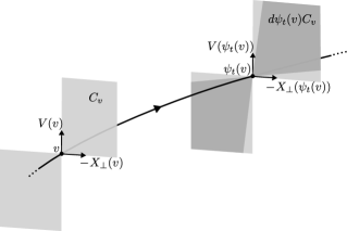
We refer the reader to, e.g., [Guillarmou:2024aa, Sect. 1.10], for the background on the contact geometry of unit tangent bundles of orientable Riemannian surfaces. Let be the geodesic flow associated with . Its orbits have the form , where is a geodesic parametrized with unit speed . The unit tangent bundle admits a frame that is orthonormal with respect to the Sasaki Riemannian metric on induced by , where is the geodesic vector field, is a unit vector field tangent to the fibers of , and . The sub-bundle of spanned by is the contact distribution of , and is invariant under the linearized geodesic flow . Donnay’s Riemannian metric has the following properties:
-
(i)
It has a contractible simple closed geodesic , which bounds an open disk .
-
(ii)
The Gaussian curvature is strictly negative on , and vanishes along .
-
(iii)
The disk is non-trapping: no forward orbit is entirely contained in the subset .
-
(iv)
The cone bundle over , given by
(5.3) is positively invariant and contracted by the linearized geodesic flow: for all and such that , we have
see Figure 3.
We recall that a closed geodesic , parametrized with unit speed and having minimal period , is hyperbolic when has an eigenvalue , and thus its eigenvalues are . The unstable bundle over is the line bundle given by
The eigenvalue is called the unstable Floquet multiplier of .
Lemma 5.4.
Let be a closed geodesic of geometrically distinct from . Then is hyperbolic, and for all such that here, is parametrized with unit speed .
Proof.
Let be a closed geodesic of geometrically distinct from . Property (iii) implies that must intersect the open set where the cone bundle is defined. We parametrize with unit speed, with in , and denote by its minimal period. Property (iv) implies that is a contraction on the space of lines (here, line means 1-dimensional vector subspace). Therefore, has a unique fixed line , which must be an eigenspace of corresponding to an eigenvalue . ∎
The parity of the Morse index of a hyperbolic closed geodesics is completely determined by their Floquet multipliers. On a Riemannian surface, a hyperbolic closed geodesic with unstable Floquet multiplier has even if and only if , namely if and only if the unstable bundle is orientable, see e.g. [Wilking:2001aa, Corollary 3.6].
Lemma 5.5.
Let be a flat-knot type relative , and two closed geodesics. Then the Morse indices and have the same parity.
Proof.
Let be the normal vector field to pointing outside . The boundary of splits as a disjoint union , where
We extend the cone field to as follows: first we extend it continuously to as in (5.3); next, for each and such that , we set
The resulting cone field on is discontinuous at , but nevertheless it is continuous (and even piecewise smooth) elsewhere. Moreover, property (iv) guarantees that has a semi-continuity with respect to the Hausdorff topology, and
Let be an isotopy from to within the relative flat knot type . We fix parametrizations depending smoothly on , and define a continuous map
We also write . An orientation on the cone bundle is a choice of connected component of which is continuous in . Notice that this notion makes sense even if is only semi-continuous. For each , the unstable bundle is contained in . Therefore is orientable if and only if is orientable, and thus if and only if the whole is orientable. We conclude that and are either both orientable or both unorientable. ∎
In order to detect homologically visible flat knot types relative , we first study the closed geodesics in the negatively curved open subset . Since is a compact surface with geodesic boundary, it is preserved by the curve shortening flow of , meaning that the evolution of any immersed loop starting inside remains in . The same holds for more classical gradient flows, for instance for the one in the setting of piecewise broken geodesics [Milnor:1963aa, Section 16], and allows Morse theoretic methods to be applied to the subspace of loops contained in .
While the statement of Theorem B involves free homotopy classes of loops in , in the next lemma we rather consider free homotopy classes of loops in , that is, connected components of .
Lemma 5.6.
In any connected component consisting of loops that are non-contractible in , there exists a unique closed geodesic of , and such a is the shortest loop in , i.e.
Proof.
Let be a connected component of loops that are non-contractible in . We fix an element that is an immersed loop and has minimal number of self-intersections. In particular, there is no non-empty subinterval such that and is a contractible loop in . Since has geodesic boundary , the curve shortening flow of preserves the compact set . Namely, the immersed loop is contained in for all . Since is non-contractible and has no subloops that are contractible in , Lemma 2.1(i) implies that converges to a closed geodesic as . Since is non-contractible, it is geometrically distinct from , and therefore it is contained in the open set . Since the Gaussian curvature is negative on , all the closed geodesics in are strict local minimizers of the length functional . If contained two geometrically distinct closed geodesics , we could define the min-max value
where the infimum ranges over the family of homotopies such that and . Standard Morse theory would imply that the value is the length of a closed geodesic in that is not a strict local minimizer of , which would give a contradiction. ∎
Lemma 5.7.
In any connected component of non-contractible loops, there exists a sequence of hyperbolic closed geodesics of with diverging length , Morse index , and such that .
Proof.
Consider an arbitrary connected component of non-contractible loops . We can find a loop that is fully contained in and has starting point . Since the closed geodesic is contractible, for each positive integer the concatenation is again a loop in . Let be the connected component of containing (Figure 4).
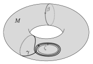
The ’s are pairwise distinct, and contain loops that are non-contractible. By Lemma 5.6, contains a unique closed geodesic , which is the shortest loop in . Since is a discrete non-compact subset of , while the space of closed geodesics in of length bounded from above by any given constant is compact, we infer that as .
We consider the min-max values
where the infimum ranges over the family of continuous homotopies , , such that and . Since the circles are strict local minimizers of the length functional , Morse theory implies that , where is a closed geodesic of 1-dimensional min-max type. Since belongs to , it is geometrically distinct from . By Lemma 5.4, in hyperbolic, and in particular non-degenerate. Therefore, has Morse index . ∎
Proof of Theorem B.
Let be a Riemannian metric on having a contractible simple closed geodesic , and a primitive free homotopy class of loops. In particular, does not contain contractible loops, and therefore does not contain nor any of its iterates. Let be Donnay Riemannian metric on having the same as simple closed geodesic. By Lemma 5.7, admits an infinite sequence of hyperbolic closed geodesics such that , , and . Since is primitive, none of the ’s is an iterated closed geodesic, and therefore we can assume that the ’s are pairwise geometrically distinct. Each has some primitive flat knot type relative . Notice that any must intersect . By Lemma 5.5, all closed geodesics of in must have odd Morse index. By Lemma 5.3, we have
and in particular contains a subgroup isomorphic to . This, together with Lemma 5.2, implies that contains a primitive closed geodesic of the original Riemannian metric . We have two possible cases:
-
•
If the family , , consists of infinitely many pairwise distinct flat knot types, then we immediately conclude that contains infinitely many primitive closed geodesics of .
-
•
If there exists a sequence of positive integers such that , then contains a subgroup isomorphic to . In particular has infinite rank. If the space of closed geodesics is not discrete, in particular it contains infinitely many closed geodesics. If instead is discrete, by Lemma 5.2 we infer
and since each local homology group has finite rank (Lemma 4.4), we infer that contains infinitely many closed geodesics. ∎
6. Birkhoff sections
6.1. From closed geodesics to Birkhoff sections
Let be a closed Riemannian surface, and its geodesic flow. For each open subset , the associated trapped set is defined as
By a convex geodesic polygon, we mean an open ball whose boundary is piecewise geodesic with at least one corner and all inner angles at its corners are less than . We stress that the closure is not required to be an embedded compact ball. Typical examples of convex geodesic polygons are the simply connected components of the complement of a finite collection of closed geodesics, as in Lemma 6.3 below.
The main result of this section is the following.
Theorem 6.1.
Any closed orientable Riemannian surface of positive genus admits a finite collection of closed geodesics whose complement satisfies , and each connected component of is a convex geodesic polygon.
In the terminology of [Contreras:2022ab, Section 4.2], the family provided by Theorem 6.1 is a “complete system of closed geodesics with empty limit subcollection”. Postponing the proof of Theorem 6.1 to the next subsection, we first derive the proof of Theorem C.
Proof of Theorem C.
Let be the finite collection of closed geodesics provided by Theorem 6.1, so that the complement satisfies , and each connected component of is a convex geodesic polygon. We fix a unit-speed parametrization , and consider a normal vector field . Each has two associated Birkhoff annuli and , defined as
Namely, is an immersed compact annulus in with boundary , and whose interior consists of those unit tangent vectors based at some point and pointing to the same side of as . Notice that is an immersed surface of section: namely, it is almost a surface of section, the only missing property being the embeddedness of into . The union
is an immersed surface of section as well.
Notice that . Since , for each there exists a minimal such that . Since each connected component of is a convex geodesic polygon, there exists a neighborhood of and such that any geodesic segment parametrized with unit speed and such that cannot be fully contained in . This readily implies that the hitting time is uniformly bounded from above by a constant for all . A surgery procedure due to Fried [Fried:1983aa], also described in the geodesics setting in [Contreras:2022ab, Section 4.1], allows to resolve the self-intersections of , and produce a surface of section with the same boundary as , contained in an arbitrarily small neighborhood of , and such that for each the orbit segment intersect . This implies that, for each , the orbit segment intersects . Therefore is a Birkhoff section. ∎
6.2. Complete system of closed geodesics
The following result, which is a special case of [Contreras:2022ab, Theorem 3.4], provides the main criterium to produce an open set with the properties asserted in Theorem 6.1.
Theorem 6.2 (Contreras, Knieper, Mazzucchelli, Schulz).
Let be a closed orientable Riemannian surface. If a convex geodesic polygon does not contain simple closed geodesics, then . ∎
In order to apply this result in the proof of Theorem 6.1 we need to detect enough closed geodesics. As a starting point, we employ the following standard family of closed geodesics, which exists on any closed orientable Riemannian surface of positive genus.
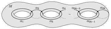
Lemma 6.3 ([Contreras:2022ab], Lemma 4.5).
On any closed orientable Riemannian surface of genus , there exist non-contractible simple closed geodesics as depicted in Figure 5. Namely, two such and intersect transversely in a single point if , they are disjoint if , and the complement is simply connected. ∎
The convex geodesic polygon may contain simple closed geodesics, and in order to apply Theorem 6.2 we need to add sufficiently many of them, as well as more closed geodesics provided by Theorem B, to our initial collection . We shall need one last statement borrowed from [Contreras:2022ab].
Lemma 6.4 ([Contreras:2022ab], Lemma 3.6).
On any closed orientable Riemannian surface , there there exists a constant with the following property: for any embedded compact annulus with and whose boundary is the disjoint union of two simple closed geodesics , we have
In a closed orientable Riemannian surface of positive genus , any contractible simple closed geodesic bounds a unique open disk . Gauss-Bonnet theorem guarantees that such a disk cannot be too small: the Gaussian curvature must attain positive values somewhere in , and the area of is bounded from below as
| (6.1) |
We denote by the family of contractible simple closed geodesics contained in the open disk . The following is the last ingredient for the proof of Theorem 6.1.
Lemma 6.5.
For each contractible simple closed geodesic such that , there exists such that .
Proof.
We set
which is a positive value according to (6.1). We fix such that
where is the constant give by Lemma 6.4. This implies that every has length . Therefore , seen as a subspace of endowed with the topology, is compact. Consider another sequence , for , such that as . By compactness, up to extracting a subsequence we have that converges in the topology to some such that . This implies that . ∎
Proof of Theorem 6.1.
Consider the family of simple closed geodesics provided by Lemma 6.3. We denote by their union, which is a path-connected compact subset of . Since every contractible simple closed geodesic bounds a disk of area uniformly bounded from below as in (6.1), Lemma 6.5 implies that there exists a maximal finite collection of pairwise disjoint contractible simple closed geodesics contained in and such that for all . We denote by their disjoint union. Here, “maximal” means that, for any other contractible simple closed geodesic contained in , the associated must contain some . If , then is the desired collection of closed geodesics: indeed, is a convex geodesic polygon that does not contain any simple closed geodesic, and Theorem 6.2 implies that .
We now consider the case . Let be an embedded loop that intersects a unique , and such intersection is transverse and consists of a single point. Theorem B implies that, for each , there exists a closed geodesic in the same free homotopy class of loops of and such that (Figure 6). Notice that must intersect too, since the intersection between and is homologically essential. We set . Since is an open ball and is path-connected, every connected component of the complement is simply connected, and thus is a convex geodesic polygon. Notice that does not contain any simple closed geodesic; indeed, if it contained a simple closed geodesic , the maximality of the collection would imply that contained some , contradicting the path-connectedness of . As before, Theorem 6.2 implies that . ∎