On reduced basis methods for eigenvalue
problems, with an application
to eigenvector continuation

Abstract.

We provide inequalities enabling to bound the error between the exact solution and an approximated solution of an eigenvalue problem, obtained by subspace projection, as in the reduced basis method. We treat self-adjoint operators and degenerate cases. We apply the bounds to the eigenvector continuation method, which consists in creating the reduced space by using basis vectors extracted from perturbation theory.

1. Introduction

A classical issue in eigenvalue problems is to reduce the number of degrees of freedom of the studied systems by extracting only the relevant ones, the full considered Hilbert space $\mathcal{H}$ being too large to be addressed in its exact form. Reduced basis method approximations aim at approximating $\mathcal{H}$ by a well-chosen low-dimensional subset $\mathcal{P}\mathcal{H}$, created via an orthogonal projector $\mathcal{P}$. Our interest here will be eigenvalue problems. Denoting the exact self-adjoint operator by $H$, then the approximated operator is

$$\left(\mathcal{P}H\mathcal{P}\right)_{\mkern 1.0mu\vrule height=6.02777pt\mkern 2.0mu\mathcal{P}\mathcal{H}\rightarrow\mathcal{P}\mathcal{H}},$$

the restriction of $H$ to $\mathcal{P}\mathcal{H}\rightarrow\mathcal{P}\mathcal{H}$, and we want to study its eigenmodes. Among other works, reduced basis problems have been investigated in [20, 19, 29], the case of several eigenvalues was examined in [15].

In Theorem 3.1, Propositions 3.2 and 3.3, we provide bounds enabling to estimate the error between the eigenmodes of the exact operator $H$ and the ones of the approximated operator $\left(\mathcal{P}H\mathcal{P}\right)_{\mkern 1.0mu\vrule height=6.02777pt\mkern 2.0mu\mathcal{P}\mathcal{H}\rightarrow\mathcal{P}\mathcal{H}}$. We treat the degenerate and almost-degenerate case by using the formalism of density matrices, and we treat the non-degenerate cases with a vector formalism. We sought to derive general bounds which could be applied to diverse settings.

We then apply our bounds to a reduced basis method which uses the derivatives of the eigenvectors to build the reduced space. Such a method was introduced in the context of computational engineering science in [24, 1, 16], and was named eigenvector continuation in [12]. Recently, many works showed the very interesting performance of this method applied to quantum physics, see for instance [18, 8, 13, 9, 26, 10, 27, 22, 11], providing perspectives to improve several areas of quantum physics. This method gives a systematic way of forming effective systems. The situation is illustrated on Figure 1, on which we represent the spectra of $H(\lambda)$ and of $\left(\mathcal{P}H(\lambda)\mathcal{P}\right)_{\mkern 1.0mu\vrule height=6.02777pt\mkern 2.0mu\mathcal{P}\mathcal{H}\rightarrow\mathcal{P}\mathcal{H}}$, where $H(\lambda)$ is the exact self-adjoint operator, depending on one parameter $\lambda\in\mathbb{R}$. Denoting one eigenvector of $H(\lambda)$ by $\phi(\lambda)$, if $\left(\frac{{\rm d}^{n}}{{\rm d}\lambda^{n}}\phi(\lambda)\right)_{\mkern 1.0mu\vrule height=6.02777pt\mkern 2.0mu\lambda=0}\in\mathcal{P}\mathcal{H}$ for all $n\in\{0,\dots,\ell\}$, it was practically remarked that the corresponding eigenmode of $\left(\mathcal{P}H(\lambda)\mathcal{P}\right)_{\mkern 1.0mu\vrule height=6.02777pt\mkern 2.0mu\mathcal{P}\mathcal{H}\rightarrow\mathcal{P}\mathcal{H}}$ is very close to the exact one, much closer than the perturbation approximation. To explain this phenomenon, quantitative bounds are provided in Corollaries 4.1 and 4.3 and in Theorem 4.9.

Figure 1. Eigenvector continuation approximates very well the targeted eigenmodes corresponding to the eigenvalue branches in red, but can fail to reproduce the other ones. One can put several eigenvectors from the Taylor series in $\mathcal{P}\mathcal{H}$ if one wants to model several eigenmodes, as on this figure where two eigenmodes in red are taken into account. In quantum physics, most of the time one is interested in only a few eigenmodes, those which are at the interface between occupied and unoccupied spectrum.

2. Definitions

We choose a standard but general mathematical setting which can address common operators involved in quantum mechanics, including Dirac operators, many-body Schrödinger operators and Bloch transforms of periodic operators.

2.1. First definitions

Let $\mathcal{H}$ be a separable Hilbert space, endowed with a scalar product $\left<\cdot,\cdot\right>$ and a corresponding norm $\left|\!\left|\cdot\right|\!\right|$. We will denote by

$$\left|\!\left|B\right|\!\right|:=\underset{\begin{subarray}{c}\psi\in\mathcal{H}\backslash\{0\}\end{subarray}}{\text{{sup}}}\;\frac{\left|\!\left|B\psi\right|\!\right|}{\left|\!\left|\psi\right|\!\right|}$$

the canonical operator norm. Let us consider a self-adjoint operator $H$ of $\mathcal{H}$, we want to approximate some of its eigenmodes by using a reduced basis method.

Let us take a self-adjoint operator $A$ of $\mathcal{H}$, possibly unbounded, which will implement the energy norm, and we consider that it has a dense domain and a dense form domain. On vectors $\varphi\in\mathcal{H}$, the energy norm is

$$\left|\!\left|\varphi\right|\!\right|_{e}:=\left|\!\left|A\varphi\right|\!\right|,$$

it is the natural norm for eigenvectors. For instance when $\mathcal{H}=L^{2}(\mathbb{R}^{3})$, in the case of a Schrödinger operator $H=-\Delta+v$, it is natural to choose $A=\sqrt{-\Delta}$ and $\left|\!\left|\cdot\right|\!\right|_{e}$ is equivalent to the Sobolev norm $H^{1}(\mathbb{R}^{3})$. We define $\left|\!\left|\cdot\right|\!\right|_{e,0}:=\left|\!\left|\cdot\right|\!\right|$ and $\left|\!\left|\cdot\right|\!\right|_{e,1}:=\left|\!\left|\cdot\right|\!\right|_{e}$, so for any $\varphi\in\mathcal{H}$ and $\delta\in\{0,1\}$, $\left|\!\left|\varphi\right|\!\right|_{e,\delta}=\left|\!\left|A^{\delta}\varphi\right|\!\right|$.

We will always assume that $c_{A}<+\infty$ and $c_{H}<+\infty$ where

$$c_{A}:=\left|\!\left|A^{-1}\right|\!\right|,\qquad c_{H}:=\left|\!\left|A^{-1}HA^{-1}\right|\!\right|.$$

2.2. Density matrices

For any $\varphi\in\mathcal{H}$, we denote by $P_{\varphi}$ the orthogonal projector onto $\mathbb{C}\varphi$. For any orthogonal projection $P$, we will use the notation $P^{\perp}:=1-P$.

The analogous objects as eigenvectors, but for degenerate systems, are density matrices of a set of eigenvectors. For any ${\bm{\varphi}}:=(\varphi_{\mu})_{\mu=1}^{\nu}\in\mathcal{H}^{\nu}$, we define the corresponding density matrix

$$\mathcal{D}_{{\bm{\varphi}}}:=\sum_{\alpha=1}^{\nu}\left|\varphi_{\alpha}\right>\left<\varphi_{\alpha}\right|=\sum_{\alpha=1}^{\nu}P_{\varphi_{\alpha}},$$

being an orthogonal projection on $\mathcal{H}$, that is $\mathcal{D}_{{\bm{\varphi}}}^{2}=\mathcal{D}_{{\bm{\varphi}}}^{*}=\mathcal{D}_{{\bm{\varphi}}}$. We denote by

$$\mathcal{U}_{\nu}:=\{U\in\mathbb{C}^{\nu\times\nu}\;|\;U^{*}U=1\}$$

the group of unitary matrices of dimension $\nu$ and for any $U\in\mathcal{U}_{\nu}$ we define its action $U{\bm{\varphi}}:=((U{\bm{\varphi}})_{\alpha})_{\alpha=1}^{\nu}$ on $\mathcal{H}^{\nu}$ where $(U{\bm{\varphi}})_{\alpha}:=\sum_{\beta=1}^{\nu}U_{\alpha\beta}\varphi_{\beta}$. We have $\mathcal{D}_{U{\bm{\varphi}}}=\mathcal{D}_{{\bm{\varphi}}}$ uniformly in $U\in\mathcal{U}_{\nu}$ and ${\bm{\varphi}}\in\mathcal{H}^{\nu}$.

For any operators $B,D$ on $\mathcal{H}$, the Hilbert-Schmidt scalar product is denoted by $\left(B,D\right)_{\text{2}}:=\operatorname{Tr}B^{*}D$ its norm $\left|\!\left|B\right|\!\right|_{2}:=\operatorname{Tr}B^{*}B$, and the corresponding normed space is the space of Hilbert-Schmidt operators, denoted by

$$\mathfrak{S}_{2}:=\{B:\mathcal{H}\rightarrow\mathcal{H},\left|\!\left|B\right|\!\right|_{2}<+\infty\}.$$ (1)

For $\delta\in\{0,1\}$ and any $B\in\mathfrak{S}_{2}$, we use the notation

$$\left|\!\left|B\right|\!\right|_{2,\delta}:=\left|\!\left|A^{\delta}B\right|\!\right|_{2}.$$ (2)

The norm $\left|\!\left|\cdot\right|\!\right|_{2,1}$, called the energy norm, is the natural one on the set of density matrices, as $\left|\!\left|\cdot\right|\!\right|_{e}$ is the natural norm on vectors.

2.3. Consider a reduced space

Let us take an orthogonal projection $\mathcal{P}$ on $\mathcal{H}$, we assume that $\mathcal{P}$ is neither the identity nor the null projection to avoid the trivial cases, and we set $\mathcal{P}^{\perp}:=1-\mathcal{P}$. The reduced space is $\mathcal{P}\mathcal{H}$, it can be infinite-dimensional, and we will need to assume that $c_{\mathcal{P}}<+\infty$ where

$$c_{\mathcal{P}}:=\left|\!\left|A\mathcal{P}A^{-1}\right|\!\right|.$$

Our central object will be $\left(\mathcal{P}\mathcal{H}\mathcal{P}\right)_{\mkern 1.0mu\vrule height=6.02777pt\mkern 2.0mu\mathcal{P}\mathcal{H}\rightarrow\mathcal{P}\mathcal{H}}:\mathcal{P}\mathcal{H}\rightarrow\mathcal{P}\mathcal{H}$, which is the restriction of $H$ to $\mathcal{P}\mathcal{H}$, hence it is an operator of $\mathcal{P}\mathcal{H}$, while $\mathcal{P}H\mathcal{P}$ is an operator of $\mathcal{H}$. If $d:=\dim\mathcal{P}\mathcal{H}$ is finite, we can see this operator as a $d\times d$ matrix. We take $\left(\mathcal{P}\mathcal{H}\mathcal{P}\right)_{\mkern 1.0mu\vrule height=6.02777pt\mkern 2.0mu\mathcal{P}\mathcal{H}\rightarrow\mathcal{P}\mathcal{H}}$ as an approximation of $H$, in the sense that its eigenmodes will well approximate the ones of $H$. Remark that since $\mathcal{P}\neq 1$, $\sigma\left(\mathcal{P}H\mathcal{P}\right)=\sigma\big{(}\left(\mathcal{P}\mathcal{H}\mathcal{P}\right)_{\mkern 1.0mu\vrule height=6.02777pt\mkern 2.0mu\mathcal{P}\mathcal{H}\rightarrow\mathcal{P}\mathcal{H}}\big{)}\cup\{0\}$ because $\operatorname{Im}\mathcal{P}^{\perp}\subset\operatorname{Ker}\mathcal{P}H\mathcal{P}$. Moreover, in our approach we avoid to use a variational point of view, so that we can reach eigenvalues having continuous spectrum below for instance.

2.4. Choose sets of eigenmodes

Take $\nu\in\mathbb{N}$, we choose a set of eigenvalues

$$\{E_{\mu}\}_{1\leqslant\mu\leqslant\nu}\in\sigma(H)$$

in the spectrum of $H$, they are counted with multiplicity and their normalized eigenvectors are denoted by $\phi_{\mu}$ and grouped into ${\bm{\phi}}:=\left(\phi_{\mu}\right)_{\mu=1}^{\nu}$. We define the associated density matrix

$$\Gamma:=\sum_{\mu=1}^{\nu}\left|\phi_{\mu}\right>\left<\phi_{\mu}\right|=\mathcal{D}_{{\bm{\phi}}}.$$

The purpose of taking $\nu\geqslant 2$ is to be able to treat the almost-degenerate and degenerate cases, i.e. when eigenvalues are close or even equal. If the eigenvalues are not close, one can take the non-degenerate case $\nu=1$ since no singular quantity will appear. Note that the eigenvalues $E_{\mu}$ are not necessarily sorted in increasing order.

For any operator $B$, we denote by $\sigma_{\textup{d}}(B)$ the discrete spectrum of $B$. Then we assume that $\left(\mathcal{P}H\mathcal{P}\right)_{\mkern 1.0mu\vrule height=6.02777pt\mkern 2.0mu\mathcal{P}\mathcal{H}\rightarrow\mathcal{P}\mathcal{H}}$ has at least $\nu$ eigenvalues in its discrete spectrum, we take $\nu$ of them, we denote them by

$$\{\mathcal{E}_{\mu}\}_{1\leqslant\mu\leqslant\nu}\subset\sigma_{\textup{d}}\big{(}\left(\mathcal{P}H\mathcal{P}\right)_{\mkern 1.0mu\vrule height=6.02777pt\mkern 2.0mu\mathcal{P}\mathcal{H}\rightarrow\mathcal{P}\mathcal{H}}\big{)},$$ (3)

we denote by $\psi_{\mu}$ the corresponding normalized eigenvectors, grouped into ${\bm{\psi}}:=\left(\psi_{\mu}\right)_{\mu=1}^{\nu}$. We define the associated density matrix

$$\Lambda:=\sum_{\mu=1}^{\nu}\left|\psi_{\mu}\right>\left<\psi_{\mu}\right|=\mathcal{D}_{{\bm{\psi}}}.$$

We will study the closeness between $\phi_{\mu}$ and $\psi_{\mu}$ for any $\mu\in\{1,\dots,\nu\}$, So to each level $\mu$ of $H$ corresponds to a level $\mu$ of $\left(\mathcal{P}H\mathcal{P}\right)_{\mkern 1.0mu\vrule height=6.02777pt\mkern 2.0mu\mathcal{P}\mathcal{H}\rightarrow\mathcal{P}\mathcal{H}}$. But they are not sorted in increasing order, so for instance if we follow a variational approach, the label $\mu$ can denote the $3^{\text{rd}}$ level of $H$ and the $5^{\text{th}}$ level of $\left(\mathcal{P}H\mathcal{P}\right)_{\mkern 1.0mu\vrule height=6.02777pt\mkern 2.0mu\mathcal{P}\mathcal{H}\rightarrow\mathcal{P}\mathcal{H}}$, and $\phi_{\mu}-\psi_{\mu}$ can be small. For example Figure 1 illustrates this principle.

2.5. Definition of partial inverses

For any self-adjoint operator $B$, if $\{e_{\mu}\}_{\mu=1}^{\alpha}\subset\sigma_{\textup{d}}(B)$, then there exists $\kappa_{B}>0$ such that

$$\left(\sigma(B)\backslash\{e_{\mu}\}_{\mu=1}^{\alpha}\right)\cap\big{(}\cup_{\mu=1}^{\alpha}\;]e_{\mu}-\kappa_{B},e_{\mu}+\kappa_{B}[\;\big{)}=\varnothing.$$ (4)

In addition to (3) we will also assume that

$$\dim\;\mathcal{P}\mathcal{H}\cap\bigoplus_{\mu=1}^{\nu}\operatorname{Ker}\big{(}\mathcal{P}H\mathcal{P}-\mathcal{E}_{\mu}\big{)}=\nu,$$ (5)

to ensure that all the eigenvectors associated to $\{\mathcal{E}_{\mu}\}_{\mu=1}^{\nu}$ are taken into account. For any $z\in\{\mathcal{E}_{\mu}\}_{\mu=1}^{\nu}\cup\left(\mathbb{C}\backslash\sigma\big{(}\left(\mathcal{P}H\mathcal{P}\right)_{\mkern 1.0mu\vrule height=6.02777pt\mkern 2.0mu\mathcal{P}\mathcal{H}\rightarrow\mathcal{P}\mathcal{H}}\big{)}\right)$ we define

$$\left(z-\mathcal{P}H\mathcal{P}\right)_{\perp}^{-1}:=\left\{\begin{array}[]{ll}\left(\left(z-\mathcal{P}H\mathcal{P}\right)_{\mkern 1.0mu\vrule height=6.02777pt\mkern 2.0mu\Lambda^{\perp}\mathcal{P}\mathcal{H}\rightarrow\Lambda^{\perp}\mathcal{P}\mathcal{H}}\right)^{-1}&\mbox{on }\Lambda^{\perp}\mathcal{P}\mathcal{H},\\ 0&\mbox{on }\Lambda\mathcal{H}\oplus\mathcal{P}^{\perp}\mathcal{H},\end{array}\right.$$ (8)

extended by linearity on $\mathcal{H}$. We also define

$$R_{\mu}:=\left(\mathcal{E}_{\mu}-\mathcal{P}H\mathcal{P}\right)_{\perp}^{-1}.$$

For any $\mu\in\{1,\dots,\nu\}$, by (3) and (4) there exists $\kappa_{\mathcal{P}H\mathcal{P}}>0$ such that $\left|\!\left|R_{\mu}\right|\!\right|\leqslant\kappa_{\mathcal{P}H\mathcal{P}}^{-1}$.

3. Main result

In this section we present our main result, which is a comparision between exact and approximated eigenmodes. It is a basic estimate that does not yet consider the parametrized setting, which is left for Section 4. We take the same notations as in Section 2.

3.1. Clusters of eigenmodes

Theorem 3.1 (Error between exact eigenmodes and reduced basis eigenmodes).

Take a Hilbert space $\mathcal{H}$, and a self-adjoint operator $A$ which is built to form a norm. Take a self-adjoint operator $H$ which eigenmodes will be approximated. Consider an orthogonal projector $\mathcal{P}$, assume that $H$ and $\mathcal{P}H\mathcal{P}$ have at least $\nu$ eigenvalues (counted with multiplicity). We consider $\nu$ eigenmodes of respectively $H$ and $\mathcal{P}H\mathcal{P}$, denoted by respectively $(E_{\mu},\phi_{\mu})$ and $(\mathcal{E}_{\mu},\psi_{\mu})$, where $\mu\in\{1,\dots,\nu\}$, ${\left|\!\left|\phi_{\mu}\right|\!\right|=\left|\!\left|\psi_{\mu}\right|\!\right|=1}$ and we assume (3) and (5). We define ${{\bm{\phi}}:=(\phi_{\mu})_{\mu=1}^{\nu}}$, ${{\bm{\psi}}:=(\psi_{\mu})_{\mu=1}^{\nu}}$, ${\Gamma:=\mathcal{D}_{{\bm{\phi}}}}$, $\Lambda:=\mathcal{D}_{{\bm{\psi}}}$. We assume that $c_{\mathcal{P}},c_{A}<+\infty$, where those quantities are defined in Section 2, and that all the quantities involved in the following are finite. For $\delta\in\{0,1\}$, we have

$$\Gamma-\Lambda=\sum_{\mu=1}^{\nu}\left((1+HR_{\mu})\mathcal{P}^{\perp}\Gamma P_{\psi_{\mu}}+\textup{s.a}\right)+\Omega,$$ (9)

where

$$\left|\!\left|\Omega\right|\!\right|_{2,\delta}\leqslant c_{A}^{\delta}\left|\!\left|\mathcal{P}^{\perp}\Gamma\right|\!\right|_{2,\delta}^{2}+\big{(}1+\left(c_{A}c_{\mathcal{P}}^{2}\right)^{\delta}\big{)}\left(1+c_{A}(1+c_{A})\left|\!\left|A\Lambda\right|\!\right|\right)^{2\delta}\left|\!\left|\Gamma-\Lambda\right|\!\right|_{2,\delta}^{2}\\ +2\left(c_{\mathcal{P}}^{\delta}+\nu c_{A}^{2\delta}|\!|\mathcal{P}^{\perp}H\Lambda|\!|\underset{\begin{subarray}{c}1\leqslant\mu\leqslant\nu\end{subarray}}{\text{{max}}}\;|\!|A^{\delta}R_{\mu}|\!|\right)\left(c_{A}\left(1+\left|\!\left|A\Lambda\right|\!\right|\right)\right)^{\delta}\left|\!\left|\mathcal{P}^{\perp}\Gamma\right|\!\right|_{2,\delta}\left|\!\left|\Gamma-\Lambda\right|\!\right|_{2,\delta}.$$ (10)

A proof is given in Section 6. The term “s.a” denotes the self adjoint operator. The next result provides another bound for $\mathcal{P}\left(\Gamma-\Lambda\right)\mathcal{P}$, using another method. For any $z\in\{E_{\mu}\}_{\mu=1}^{\nu}\cup\left(\mathbb{C}\backslash\sigma(H)\right)$ we define

$$\left(z-H\right)_{\perp}^{-1}:=\left\{\begin{array}[]{ll}\left(\left(z-H\right)_{\mkern 1.0mu\vrule height=6.02777pt\mkern 2.0mu\Gamma^{\perp}\mathcal{H}\rightarrow\Gamma^{\perp}\mathcal{H}}\right)^{-1}&\mbox{on }\Gamma^{\perp}\mathcal{H},\\ 0&\mbox{on }\Gamma\mathcal{H}\end{array}\right.$$ (13)

extended by linearity on $\mathcal{H}$.

Proposition 3.2 (Another bound for $\mathcal{P}\left(\Gamma-\Lambda\right)\mathcal{P}$).

Let us make the same assumption as in Theorem 3.1, and moreover assume that

$$\operatorname{dist}\left(\{\mathcal{E}_{\mu}\}_{\mu=1}^{\nu},\sigma_{\textup{d}}\big{(}H_{\mkern 1.0mu\vrule height=6.02777pt\mkern 2.0mu\Gamma^{\perp}\mathcal{H}\rightarrow\Gamma^{\perp}\mathcal{H}}\big{)}\right) >0,$$

$$\operatorname{dist}\left(\{E_{\mu}\}_{\mu=1}^{\nu},\sigma_{\textup{d}}\big{(}\left(\mathcal{P}H\mathcal{P}\right)_{\mkern 1.0mu\vrule height=6.02777pt\mkern 2.0mu\Lambda^{\perp}\mathcal{P}\mathcal{H}\rightarrow\Lambda^{\perp}\mathcal{P}\mathcal{H}}\big{)}\right) >0.$$ (14)

Then

$$\left|\!\left|\Gamma-\Lambda\right|\!\right|_{2,\delta}\leqslant c_{A}^{\delta}\left|\!\left|\mathcal{P}^{\perp}\Gamma\right|\!\right|_{2,\delta}^{2}+\nu c_{\mathcal{P}}^{\delta}\left(\underset{\begin{subarray}{c}1\leqslant\mu\leqslant\nu\end{subarray}}{\text{{max}}}\;\left|\!\left|A^{\delta}\left(\mathcal{E}_{\mu}-H\right)_{\perp}^{-1}\right|\!\right|\right)\left|\!\left|\mathcal{P}^{\perp}H\Lambda\right|\!\right|\\ +\left(c_{A}c_{\mathcal{P}}\left|\!\left|A\Gamma\right|\!\right|\right)^{\delta}\left(2+\nu\underset{\begin{subarray}{c}1\leqslant\mu\leqslant\nu\end{subarray}}{\text{{max}}}\;\left|\!\left|\left(E_{\mu}-\mathcal{P}H\mathcal{P}\right)_{\perp}^{-1}H\mathcal{P}^{\perp}\right|\!\right|\right)\left|\!\left|\mathcal{P}^{\perp}\Gamma\right|\!\right|_{2,\delta}.$$ (15)

The proof of this result is provided in Section 6.

3.2. One eigenmode

In the case where we treat only one eigenmode, one can obtain more precision about the errors, this is the object of the following result. We drop the subscripts 1 labeling the different eigenvectors, because we consider only one of them and write $\phi:=\phi_{1}$, $\psi:=\psi_{1}$, $E:=E_{1}$, $\mathcal{E}:=\mathcal{E}_{1}$, and $R:=R_{1}$.

Proposition 3.3 (Further detail in the non-degenerate case).

Make the same assumptions as in Theorem 3.1, take $\nu=1$ and remove the subscripts $1$. Thus $(E,\phi)$ is an eigenmode of $H$ and $(\mathcal{E},\psi)$ is an eigenmode of $\left(\mathcal{P}H\mathcal{P}\right)_{\mkern 1.0mu\vrule height=6.02777pt\mkern 2.0mu\mathcal{P}\mathcal{H}\rightarrow\mathcal{P}\mathcal{H}}$. In a gauge where $\left<\psi,\phi\right>\in\mathbb{R}$,

$$\phi-\psi =\left(1+RH\right)\mathcal{P}^{\perp}\phi-\tfrac{1}{2}\left|\!\left|\phi-\psi\right|\!\right|^{2}\psi+\left(\mathcal{E}-E\right)R\left(\phi-\psi\right),$$ (16)

$$E-\mathcal{E} =\left<\mathcal{P}^{\perp}\phi,\left(\mathcal{E}-H\right)\left(1+RH\right)\mathcal{P}^{\perp}\phi\right>+(E-\mathcal{E})\left|\!\left|\phi-\psi\right|\!\right|^{2}$$

$$-\left|\!\left|\phi-\psi\right|\!\right|^{2}\operatorname{Re}\left<\mathcal{P}^{\perp}\phi,(H-E)(\phi-\psi)\right>+\left(E-\mathcal{E}\right)^{2}\left<\phi-\psi,R\left(\phi-\psi\right)\right>.$$ (17)

The proof is presented in Section 7.

3.3. Remarks

Let us now proceed with some remarks.

Remark 3.4 (Leading term in $\Gamma-\Lambda$).

Since $\mathcal{P}^{\perp}\Lambda=0$, we have

$$\left|\!\left|\mathcal{P}^{\perp}\Gamma\right|\!\right|_{2,\delta}=\left|\!\left|A^{\delta}\mathcal{P}^{\perp}A^{-\delta}A^{\delta}\left(\Gamma-\Lambda\right)\right|\!\right|_{2,\delta}\leqslant(1+c_{\mathcal{P}})^{\delta}\left|\!\left|\Gamma-\Lambda\right|\!\right|_{2,\delta},$$

hence we see in (10) that $\Omega$ is quadratic in $\left|\!\left|\Gamma-\Lambda\right|\!\right|_{2,\delta}$, and thus negligible in (9) when $\left|\!\left|\Gamma-\Lambda\right|\!\right|_{2,\delta}$ is small. The leading term for $\Gamma-\Lambda$ is thus $\sum_{\mu=1}^{\nu}\left((1+HR_{\mu})\mathcal{P}^{\perp}\Gamma P_{\psi_{\mu}}+\textup{s.a}\right)$, as emphazised in (9).

Remark 3.5 (Invariance under unitary transforms).

All the quantities involved in (9) and (10) and (15) are invariant under the transformations ${\bm{\phi}}\rightarrow U{\bm{\phi}}$ and ${\bm{\psi}}\rightarrow V{\bm{\psi}}$, where $U,V\in\mathcal{U}_{\nu}$.

Remark 3.6 (Main consequences of Theorem 3.1).

From Theorem 3.1, for $\left|\!\left|\Gamma-\Lambda\right|\!\right|_{2,\delta}$ small enough, and $\delta\in\{0,1\}$,

$$\left|\!\left|\Gamma-\Lambda\right|\!\right|_{2,\delta}\leqslant 4\nu\left(c_{A}\left|\!\left|A\Lambda\right|\!\right|\right)^{\delta}\left|\!\left|\mathcal{P}^{\perp}\Gamma\right|\!\right|_{2,\delta}\underset{\begin{subarray}{c}1\leqslant\mu\leqslant\nu\end{subarray}}{\text{{max}}}\;\left|\!\left|A^{\delta}(1+R_{\mu}H)\mathcal{P}^{\perp}A^{-\delta}\right|\!\right|,$$ (18)

see Section 7.3 to have more details on how to obtain this inequality. Moreover, by Lemma B.1, there exists a rotation $U\in\mathcal{U}_{\nu}$ such that

$$\sum_{\mu=1}^{\nu}\left|\!\left|A\big{(}{\bm{\phi}}_{\mu}-\left(U{\bm{\psi}}\right)_{\mu}\big{)}\right|\!\right|\leqslant c\left|\!\left|A\mathcal{P}^{\perp}\Gamma\right|\!\right|_{2}$$ (19)

for some constant $c$, and again by Lemma B.1, and yet for another constant $c$, the error in the sums of eigenvalues is quadratic, that is

$$\left|\sum_{\mu=1}^{\nu}\left(E_{\mu}-\mathcal{E}_{\mu}\right)\right|\leqslant c\left|\!\left|A\mathcal{P}^{\perp}\Gamma\right|\!\right|_{2}^{2}.$$ (20)

Hence those errors are controled by the key quantity $\left|\!\left|A\mathcal{P}^{\perp}\Gamma\right|\!\right|$.

Remark 3.7 (Main consequences of Proposition 3.3).

If $\left|\!\left|\phi-\psi\right|\!\right|_{e}$ is small enough, then Proposition 3.3 yields

$$\left|\!\left|\phi-\psi\right|\!\right|_{e} \leqslant 2\left(1+c_{H}\left|\!\left|ARA\right|\!\right|\right)\left|\!\left|A\mathcal{P}^{\perp}\phi\right|\!\right|,$$ (21)

$$\left|E-\mathcal{E}\right| \leqslant 4\left(c_{H}+c_{A}^{2}\left|E\right|\right)\left(1+c_{H}\left|\!\left|ARA\right|\!\right|\right)^{2}\left|\!\left|A\mathcal{P}^{\perp}\phi\right|\!\right|^{2},$$ (22)

see Section 7.3 to have more details on the derivation of those inequalities. Thus those errors are controlled by the key quantity $\left|\!\left|A\mathcal{P}^{\perp}\phi\right|\!\right|$.

Remark 3.8 (About the smallness of the different terms in (16) and (17)).

The term $\mathcal{P}^{\perp}\phi=\mathcal{P}^{\perp}\left(\phi-\psi\right)$ is controled by $\left|\!\left|\phi-\psi\right|\!\right|_{e}$ in norm. When $\left|\!\left|\phi-\psi\right|\!\right|_{e}$ is small, in (16) the leading term is $\left(1+RH\right)\mathcal{P}^{\perp}\phi$, then the second term is of order 2 and $\left(\mathcal{E}-E\right)R\left(\phi-\psi\right)$ is of order 3. In (17), the leading term is $\left<\mathcal{P}^{\perp}\phi,\left(\mathcal{E}-H\right)\left(1+RH\right)\mathcal{P}^{\perp}\phi\right>$ (which is of order 2), the second term is of order 4, the third term is of order 4 and the last one of order 6.

Remark 3.9 (Making $\mathcal{P}$ grow improves the error, in general).

Consider the vector case corresponding to Proposition 3.3. We numerically see that making $\mathcal{P}$ larger by adding more vectors to $\mathcal{P}\mathcal{H}$ decreases the error, in general. This can be expected from the form of the leading term $\left(1+RH\right)\mathcal{P}^{\perp}\phi$, in which, for any vector $\varphi\in\mathcal{H}$, $\mathcal{P}^{\perp}\varphi$ decreases. However, as will be seen in Section 5, there are some exceptional cases where making $\mathcal{P}$ larger increases the error.

Remark 3.10 (Difference between (9) and (15)).

The quantity $\mathcal{P}^{\perp}H\Lambda$ can be interpreted as an a posteriori one. When $\Gamma$ is close to $\Lambda$ it is small because, since $[H,\Gamma]=0$ and $\mathcal{P}^{\perp}\Lambda=0$, then $\mathcal{P}^{\perp}H\Lambda=\mathcal{P}^{\perp}[H,\Lambda-\Gamma]$. The bound (10) involves $\left|\!\left|\Gamma-\Lambda\right|\!\right|_{2,\delta}^{2}$ while (15) does not. If one rather needs a posteriori quantification,  (15) might be better.

4. Application to eigenvector continuation

We now put the results of the previous section in the context of the eigenvector continuation. We refer to Figure 1 to illustrate our reasoning.

4.1. Definitions and assumptions

We start by introducing some definitions and making some assumptions, which will enable to apply Rellich’s theorem and Theorems 3.1 and 3.3.

4.1.1. Analytic family of operators

We present here assumptions which will be sufficient to use the Rellich theorem on the existence of analytic eigenmodes.

Let us take a self-ajoint operator $H^{0}$ such that $\sigma(H^{0})\neq\mathbb{R}$, so there exists $r\in\mathbb{R}$ and $\varepsilon>0$ such that

$$\sigma(H^{0})\,\cap\,]r-\varepsilon,r+\varepsilon[\,=\varnothing.$$ (23)

Let us take a self-adjoint energy norm operator $A$, for instance one can take $A=\left|H^{0}-r\right|^{\frac{1}{2}}$. We will choose a simple case for the family of operators, that is we consider $M\in\mathbb{N}\cup\{0\}$, a series of self-adjoint operators $H^{n}$ for $n\in\{0,\dots,M\}$ such that

$$D(H^{0})\subset D(H^{n})$$ (24)

where $D(\cdot)$ denotes the domain of an operator, and such that

$$\underset{\begin{subarray}{c}n\in\mathbb{N}\end{subarray}}{\text{{sup}}}\;\left|\!\left|H^{n}\left(H^{0}-r\right)^{-1}\right|\!\right|<+\infty,\qquad\underset{\begin{subarray}{c}n\in\mathbb{N}\cup\{0\}\end{subarray}}{\text{{max}}}\;\left|\!\left|A^{-1}H^{n}A^{-1}\right|\!\right|<+\infty.$$ (25)

For instance, one can take $H^{n}$ as bounded operators for any $n\in\{1,\dots,M\}$. We also define $H^{n}:=0$ for any $n\geqslant M+1$. Finally, we define

$$H(\lambda):=\sum_{n=0}^{+\infty}\lambda^{n}H^{n}.$$

4.1.2. Choose a set of eigenvalues of $H(\lambda)$

Let us assume that $H^{0}$ has at least $\nu$ eigenvalues

$$\{E_{\mu}^{0}\}_{\mu=1}^{\nu}\subset\sigma_{\text{d}}(H^{0})$$ (26)

in the discrete spectrum, counted with multiplicity but not necessarily sorted in increasing order. By (4), there exists $\kappa_{H^{0}}>0$ such that

$$\left(\sigma(H^{0})\backslash\{E_{\mu}^{0}\}_{\mu=1}^{\nu}\right)\cap\big{(}\cup_{\mu=1}^{\nu}\;]E_{\mu}^{0}-\kappa_{H^{0}},E_{\mu}^{0}+\kappa_{H^{0}}[\;\big{)}=\varnothing,$$ (27)

and assume that

$$\dim\;\bigoplus_{\mu=1}^{\nu}\operatorname{Ker}\left(H^{0}-E_{\mu}^{0}\right)=\nu.$$ (28)

Rellich’s theorem states that the eigenmodes of $H(\lambda)$ are also analytic in $\lambda$, see [25, Theorem XII.3 p4], [25, Problem XII.17, p71], [28, Theorem 1.4.4 p25] and [3, Theorem 1 p21] for instance. The extension to infinite-dimensional space also holds under some technical assumptions, see [17],  [25, Lemma p16],  [25, Theorem XII.8 p15] and [25, Theorem XII.13 p22].

We denote by $\left(E_{\mu}(\lambda),\phi_{\mu}(\lambda)\right)$ the eigenmodes, analytic in $\lambda$, respecting $E_{\mu}(\lambda)=E^{0}_{\mu}$ and $\left<\phi_{\mu}(\lambda),\phi_{\alpha}(\lambda)\right>=\delta_{\mu\alpha}$ for any $\mu,\alpha\in\{1,\dots,\nu\}$. The phasis of the vectors is not fixed by those conditions, meaning that taking smooth maps $\theta_{\mu}:\mathbb{R}\rightarrow\mathbb{R}$, the eigenvectors $e^{i\theta_{\mu}(\lambda)}\phi_{\mu}(\lambda)$ also respect the previous conditions.

For any $\lambda\in]-\lambda_{0},\lambda_{0}[$, we define $\Gamma(\lambda):=\mathcal{D}_{{\bm{\phi}}(\lambda)}$ and the partial inverse

$$K_{\mu}(0):=\left\{\begin{array}[]{ll}\left(\left(E_{\mu}(0)-H(0)\right)_{\mkern 1.0mu\vrule height=6.02777pt\mkern 2.0mu\left(\Gamma(0)\right)^{\perp}\mathcal{H}\rightarrow\left(\Gamma(0)\right)^{\perp}\mathcal{H}}\right)^{-1}&\mbox{on }(\Gamma(0))^{\perp}\mathcal{H},\\ 0&\mbox{on }\Gamma(0)\mathcal{H},\end{array}\right.$$ (31)

extended by linearity on $\mathcal{H}$. By (27) we have $\left|\!\left|K_{\mu}(0)\right|\!\right|\leqslant\kappa_{H^{0}}^{-1}$, and we assume that

$$\underset{\begin{subarray}{c}1\leqslant\mu\leqslant\nu\end{subarray}}{\text{{max}}}\;\left|\!\left|AK_{\mu}(0)A\right|\!\right|<+\infty.$$ (32)

4.1.3. Starting point for $\left(\mathcal{P}H(\lambda)\mathcal{P}\right)_{\mkern 1.0mu\vrule height=6.02777pt\mkern 2.0mu\mathcal{P}\mathcal{H}\rightarrow\mathcal{P}\mathcal{H}}$

The starting point of the analysis of the reduced operator will be $\lambda=0$, on which the eigenmodes under study of the exact and reduced operators are equal. So the first step consists in exploiting this fact.

Let us consider an orthogonal projection $\mathcal{P}$, where $\mathcal{P}\mathcal{H}$ can be infinite-dimensional. The hypothesis of eigenvector continuation, which we will see later, imply that the exact eigenvector $\phi_{\mu}(0)$ belongs to $\mathcal{P}\mathcal{H}$, hence $\mathcal{P}H(0)\mathcal{P}\phi_{\mu}(0)=E_{\mu}(0)\phi_{\mu}(0)$, so $\phi_{\mu}(0)$ is also an eigenvector of $(\mathcal{P}H(0)\mathcal{P})_{\mathcal{P}\mathcal{H}\rightarrow\mathcal{P}\mathcal{H}}$ with eigenvalue $E_{\mu}(0)$. We need to assume that

$$\{E_{\mu}(0)\}_{\mu=1}^{\nu}\subset\sigma_{\text{d}}\big{(}\left(\mathcal{P}H(0)\mathcal{P}\right)_{\mkern 1.0mu\vrule height=6.02777pt\mkern 2.0mu\mathcal{P}\mathcal{H}\rightarrow\mathcal{P}\mathcal{H}}\big{)}$$ (33)

and

$$\dim\;\mathcal{P}\mathcal{H}\cap\bigoplus_{\mu=1}^{\nu}\operatorname{Ker}(\mathcal{P}H(0)\mathcal{P}-E_{\mu}(0))=\nu.$$ (34)

Those last assumptions mean that the reduction from $\mathcal{H}$ to $\mathcal{P}\mathcal{H}$ does not produce spectral pollution close to the $E_{\mu}(0)$’s for $H(0)$.

4.1.4. Analytic branches for $\left(\mathcal{P}H(\lambda)\mathcal{P}\right)_{\mkern 1.0mu\vrule height=6.02777pt\mkern 2.0mu\mathcal{P}\mathcal{H}\rightarrow\mathcal{P}\mathcal{H}}$

To be able to apply Rellich’s theorem for $\left(\mathcal{P}H(\lambda)\mathcal{P}\right)_{\mkern 1.0mu\vrule height=6.02777pt\mkern 2.0mu\mathcal{P}\mathcal{H}\rightarrow\mathcal{P}\mathcal{H}}$, we make several assumptions. Let us assume that $\sigma\left(\left(\mathcal{P}H(\lambda)\mathcal{P}\right)_{\mkern 1.0mu\vrule height=6.02777pt\mkern 2.0mu\mathcal{P}\mathcal{H}\rightarrow\mathcal{P}\mathcal{H}}\right)\neq\mathbb{R}$, so there exists $r_{\mathcal{P}}\in\mathbb{R}$ and $\varepsilon_{\mathcal{P}}>0$ such that

$$\sigma\left(\left(\mathcal{P}H(\lambda)\mathcal{P}\right)_{\mkern 1.0mu\vrule height=6.02777pt\mkern 2.0mu\mathcal{P}\mathcal{H}\rightarrow\mathcal{P}\mathcal{H}}\right)\,\cap\,]r_{\mathcal{P}}-\varepsilon_{\mathcal{P}},r_{\mathcal{P}}+\varepsilon_{\mathcal{P}}[\,=\varnothing,$$ (35)

assume that

$$\underset{\begin{subarray}{c}n\in\mathbb{N}\end{subarray}}{\text{{sup}}}\;\left|\!\left|\mathcal{P}H^{n}\mathcal{P}\left(\left(\mathcal{P}H^{0}\mathcal{P}-r_{\mathcal{P}}\right)_{\mkern 1.0mu\vrule height=6.02777pt\mkern 2.0mu\mathcal{P}\mathcal{H}\rightarrow\mathcal{P}\mathcal{H}}\right)^{-1}\right|\!\right|<+\infty.$$ (36)

and that for any $n\in\mathbb{N}$,

$$D(\mathcal{P}H^{0}\mathcal{P})\subset D(\mathcal{P}H^{n}\mathcal{P}).$$ (37)

Rellich’s theorem ensures the existence of $\nu$ eigenmodes $\left(\mathcal{E}_{\mu}(\lambda),\psi_{\mu}(\lambda)\right)_{\mu=1}^{\nu}$ of $\left(\mathcal{P}H(\lambda)\mathcal{P}\right)_{\mkern 1.0mu\vrule height=6.02777pt\mkern 2.0mu\mathcal{P}\mathcal{H}\rightarrow\mathcal{P}\mathcal{H}}$, analytic in $\lambda\in]-\lambda_{0},\lambda_{0}[$ where $\lambda_{0}>0$, such that $\mathcal{E}_{\mu}(0)=E_{\mu}(0)$, $\psi_{\mu}(0)=\phi_{\mu}(0)$ and $\left<\psi_{\mu}(\lambda),\psi_{\alpha}(\lambda)\right>=\delta_{\mu\alpha}$ for any $\mu,\alpha\in\{1,\dots,\nu\}$. We take $\lambda_{0}$ small enough so that for some $\kappa_{H}>0$ (which does not depend on $\lambda$) and any $\lambda\in]-\lambda_{0},\lambda_{0}[$,

$$\big{(}\sigma\big{(}\left(\mathcal{P}H(\lambda)\mathcal{P}\right)_{\mkern 1.0mu\vrule height=6.02777pt\mkern 2.0mu\mathcal{P}\mathcal{H}\rightarrow\mathcal{P}\mathcal{H}}\big{)}\backslash\{\mathcal{E}_{\mu}(\lambda)\}_{\mu=1}^{\nu}\big{)}\\ \cap\big{(}\cup_{\mu=1}^{\nu}\;]\mathcal{E}_{\mu}(\lambda)-\kappa_{H},\mathcal{E}_{\mu}(\lambda)+\kappa_{H}[\;\big{)}=\varnothing,$$ (38)

meaning that the rest of the spectrum remains far from $\{\mathcal{E}_{\mu}(\lambda)\}_{\mu=1}^{\nu}$, uniformly in $\lambda$. Together with (34), this implies that for any $\lambda\in]-\lambda_{0},\lambda_{0}[$,

$$\dim\;\mathcal{P}\mathcal{H}\cap\bigoplus_{\mu=1}^{\nu}\operatorname{Ker}(\mathcal{P}H(\lambda)\mathcal{P}-E_{\mu}(\lambda))=\nu.$$

For any $\lambda\in]-\lambda_{0},\lambda_{0}[$ we can hence define

$$R_{\mu}(\lambda)\\ :=\left\{\begin{array}[]{ll}\left(\left(\mathcal{E}_{\mu}(\lambda)-\mathcal{P}H(\lambda)\mathcal{P}\right)_{\mkern 1.0mu\vrule height=6.02777pt\mkern 2.0mu\Lambda(\lambda)^{\perp}\mathcal{P}\mathcal{H}\rightarrow\Lambda(\lambda)^{\perp}\mathcal{P}\mathcal{H}}\right)^{-1}&\mbox{on }\Lambda(\lambda)^{\perp}\mathcal{P}\mathcal{H},\\ 0&\mbox{on }\Lambda(\lambda)\mathcal{H}\oplus\mathcal{P}^{\perp}(\lambda)\mathcal{H},\end{array}\right.$$ (39)

extended by linearity on $\mathcal{H}$. From (38) we have $\left|\!\left|R_{\mu}(\lambda)\right|\!\right|\leqslant\kappa^{-1}_{H(\lambda)}$.

4.2. Statement of the results

For any $\lambda\in]-\lambda_{0},\lambda_{0}[$, we recall that $\Gamma(\lambda):=\mathcal{D}_{{\bm{\phi}}(\lambda)}$. For any $n\in\mathbb{N}\cup\{0\}$ and any $\mu\in\{1,\dots,\nu\}$,

$$\phi_{\mu}^{n}:=\left(\frac{{\rm d}^{n}}{{\rm d}\lambda^{n}}\phi_{\mu}(\lambda)\right)_{\mkern 1.0mu\vrule height=6.02777pt\mkern 2.0mu\lambda=0},\qquad\qquad\Gamma^{n}:=\left(\frac{{\rm d}^{n}}{{\rm d}\lambda^{n}}\Gamma(\lambda)\right)_{\mkern 1.0mu\vrule height=6.02777pt\mkern 2.0mu\lambda=0}.$$ (40)

See Proposition 9.1 to see how to obtain the $\Gamma^{n}$’s. Let us also define

$$\xi_{\textup{ec},\ell,\delta}^{\textup{deg}} :=\left|\!\left|\sum_{\mu=1}^{\nu}\left(1+R_{\mu}(0)H(0)\right)\mathcal{P}^{\perp}\Gamma^{\ell+1}P_{\phi_{\mu}(0)}+\text{s.a}\right|\!\right|_{2,\delta}.$$

The main theorem of this section is about the closeness of the density matrix $\Gamma(\lambda)$ associated to the exact operator $H(\lambda)$ with the one of the approximate operator $\left(\mathcal{P}H(\lambda)\mathcal{P}\right)_{\mkern 1.0mu\vrule height=6.02777pt\mkern 2.0mu\mathcal{P}\mathcal{H}\rightarrow\mathcal{P}\mathcal{H}}$, when $\mathcal{P}\mathcal{H}$ contains the first $\ell+1$ derivatives of $\Gamma(\lambda)$.

Corollary 4.1 (Eigenvector continuation in the perturbative regime, for clusters of eigenmodes).

As in Section 4.1.1, consider a Hamiltonian family $H(\lambda):=\sum_{n=0}^{M}\lambda^{n}H^{n}$ and consider $\nu$ analytic families of eigenmodes $\left(E_{\mu}(\lambda),\phi_{\mu}(\lambda)\right)_{\mu=1}^{\nu}$ with $\left<\phi_{\mu}(\lambda),\phi_{\alpha}(\lambda)\right>{}=\delta_{\mu\alpha}$. Make the presented assumptions (23), (24), (25), (26), (32), (28), (33), (34), (35), (36), (37) and (38). Consider an orthogonal projector $\mathcal{P}$, satisfying (33),  (34). Then, there are $\nu$ eigenmodes $\left(\mathcal{E}_{\mu}(\lambda),\psi_{\mu}(\lambda)\right)_{\mu=1}^{\nu}$ of $\left(\mathcal{P}H(\lambda)\mathcal{P}\right)_{\mkern 1.0mu\vrule height=6.02777pt\mkern 2.0mu\mathcal{P}\mathcal{H}\rightarrow\mathcal{P}\mathcal{H}}$, analytic in $\lambda$ such that $\mathcal{E}_{\mu}(0)=E_{\mu}(0)$, $\psi_{\mu}(0)=\phi_{\mu}(0)$ and $\left<\psi_{\mu}(\lambda),\psi_{\alpha}(\lambda)\right>{}=\delta_{\mu\alpha}$ for any $\mu,\alpha\in\{1,\dots,\nu\}$. We define ${\bm{\phi}}(\lambda):=\left(\phi(\lambda)\right)_{\mu=1}^{\nu}$, ${\bm{\psi}}(\lambda):=\left(\psi(\lambda)\right)_{\mu=1}^{\nu}$, $\Gamma(\lambda):=\mathcal{D}_{{\bm{\phi}}(\lambda)}$ and $\Lambda(\lambda):=\mathcal{D}_{{\bm{\psi}}(\lambda)}$. Given $\ell\in\mathbb{N}\cup\{0\}$, if

$$\forall n\in\{0,\dots,\ell\},\qquad\operatorname{Im}\Gamma^{n}\subset\mathcal{P}\mathcal{H},$$ (41)

then there exists $\lambda_{0}>0$ such that for any $\lambda\in]-\lambda_{0},\lambda_{0}[$ and $\delta\in\{0,1\}$,

$$\left|\left|\!\left|\Gamma(\lambda)-\Lambda(\lambda)\right|\!\right|_{2,\delta}-\left|\lambda\right|^{\ell+1}\xi^{\textup{deg}}_{\textup{ec},\ell,\delta}\right| \leqslant c\left(\left|\lambda\right|b\right)^{\ell+2},$$ (42)

where $b$ and $c$ are independent of $\lambda$ and $\ell$.

We give a proof in Section 10. Proposition 9.1 recalls the results of[21] showing how to obtain $\Gamma^{n}$. The next result provides a practical way of building the reduced space used in (41), via an explicit and simple basis.

Lemma 4.2 (Building the reduced space for density matrices).

Consider the context of Corollary 4.1. Take $(\varphi_{\mu})_{\mu=1}^{\nu}\in\mathcal{H}^{\nu}$ to be a basis of the unperturbed space $\oplus_{\mu=1}^{\nu}\operatorname{Ker}\left(H(0)-E_{\mu}(0)\right)$. Then

$$\bigoplus_{n=0}^{\ell}\operatorname{Im}\Gamma^{n}=\operatorname{Span}\left(\Gamma^{n}\varphi_{\mu}\;|\;0\leqslant n\leqslant\ell,1\leqslant\mu\leqslant\nu\right).$$

A proof is provided in Section 10.

We now discuss the vector case and as in Proposition 3.3 we drop the subscripts 1, so $R(\lambda):=R_{1}(\lambda)$, $\phi(\lambda):=\phi_{1}(\lambda)$, $\psi(\lambda):=\psi_{1}(\lambda)$, $E(\lambda):=E_{1}(\lambda)$, $\mathcal{E}(\lambda):=\mathcal{E}_{1}(\lambda)$, $\phi^{n}:=\phi^{n}_{1}$. We define

$$\xi_{\textup{ec},\ell,\delta}^{\textup{nd},V} :=\left|\!\left|\left(1+R(0)H(0)\right)\mathcal{P}^{\perp}\phi^{\ell+1}\right|\!\right|_{e,\delta}$$

$$\xi_{\textup{ec},\ell}^{\textup{nd},E} :=\left|\left<\mathcal{P}^{\perp}\phi^{\ell+1},(H(0)-E(0))\left(1+R(0)H(0)\right)\mathcal{P}^{\perp}\phi^{\ell+1}\right>\right|.$$

We now state the corresponding result but in the non-degenerate case and for vectors.

Corollary 4.3 (Eigenvector continuation in the perturbative regime, one eigenmode).

We make the same assumptions as in Corollary 4.1, we take $\nu=1$ and remove the subscripts 1, and we take $\ell\in\mathbb{N}\cup\{0\}$. We choose the phasis of $\phi(\lambda)$ and $\psi(\lambda)$ such that $\left<\phi^{0},\phi(\lambda)\right>\in\mathbb{R}_{+}$ and $\left<\phi(\lambda),\psi(\lambda)\right>\in\mathbb{R}$. If

$$\forall n\in\{0,\dots,\ell\},\qquad\left(\tfrac{{\rm d}^{n}}{{\rm d}\lambda^{n}}\phi(\lambda)\right)_{\mkern 1.0mu\vrule height=6.02777pt\mkern 2.0mu\lambda=0}\in\mathcal{P}\mathcal{H},$$ (43)

then there exists $\lambda_{0}>0$ such that for any $\lambda\in]-\lambda_{0},\lambda_{0}[$ and $\delta\in\{0,1\}$,

$$\left|\left|\!\left|\phi(\lambda)-\psi(\lambda)\right|\!\right|_{e,\delta}-\left|\lambda\right|^{\ell+1}\xi^{\textup{nd,vec}}_{\textup{ec},\ell,\delta}\right| \leqslant c\left(\left|\lambda\right|b\right)^{\ell+2},$$ (44)

$$\left|\left|E(\lambda)-\mathcal{E}(\lambda)\right|-\left|\lambda\right|^{2(\ell+1)}\xi^{\textup{nd},E}_{\textup{ec},\ell}\right| \leqslant c\left(\left|\lambda\right|b\right)^{2\ell+3},$$ (45)

where $b$ and $c$ are independent of $\lambda$ and $\ell$.

We provide a proof in Section 10.

4.3. Remarks

Now, several remarks seem in order.

Remark 4.4 (Error with explicit constant).

Inequality (44) could be written as

$$\left|\!\left|\phi(\lambda)-\psi(\lambda)\right|\!\right|_{e,\delta}=\left|\lambda\right|^{\ell+1}\xi^{\textup{nd,vec}}_{\textup{ec},\ell,\delta}+O\left(\left(\left|\lambda\right|b\right)^{\ell+2}\right),$$

where $O(\cdot)$ would be a function bounded in $\lambda$ and $\ell$.

Remark 4.5 (Equality of perturbation terms).

A consequence of (44) and (45) is that for all $n\in\{0,\dots,\ell\},k\in\{0,\dots,2\ell+1\}$,

$$\left(\tfrac{{\rm d}^{n}}{{\rm d}\lambda^{n}}\psi(\lambda)\right)_{\mkern 1.0mu\vrule height=6.02777pt\mkern 2.0mu\lambda=0}=\left(\tfrac{{\rm d}^{n}}{{\rm d}\lambda^{n}}\phi(\lambda)\right)_{\mkern 1.0mu\vrule height=6.02777pt\mkern 2.0mu\lambda=0},\qquad\left(\tfrac{{\rm d}^{k}}{{\rm d}\lambda^{k}}\mathcal{E}(\lambda)\right)_{\mkern 1.0mu\vrule height=6.02777pt\mkern 2.0mu\lambda=0}=\left(\tfrac{{\rm d}^{k}}{{\rm d}\lambda^{k}}E(\lambda)\right)_{\mkern 1.0mu\vrule height=6.02777pt\mkern 2.0mu\lambda=0},$$

meaning that the first perturbation terms of eigenvector continuation are the same as the ones of the exact problem.

Remark 4.6 (Intermediate normalization).

Intermediate normalization is reviewed in Appendix A. Instead of building the reduced space $\mathcal{P}\mathcal{H}$ from the $\phi^{n}$’s, one can form it by using the eigenvectors in intermediate normalization, denoted by $\Phi^{n}$. Using this last normalization is more convenient because it involves less computations. From (137) we have

$$\operatorname{Span}\left(\Phi^{k},\;0\leqslant k\leqslant\ell\right)=\operatorname{Span}\left(\phi^{k},\;0\leqslant k\leqslant\ell\right).$$ (46)

Hence one can form the reduced space of eigenvector continuation by using either intermediate or unit normalization perturbation vectors, this is equivalent.

Remark 4.7 (Comparision to perturbation theory).

We provide a comparision of eigenvector continuation with perturbation theory in Section 5.

Remark 4.8 (Generalization to higher-dimensional parameter space).

Corollary 4.1 is stated for a one-dimensional parameter space, parametrized by $\lambda$, but one can straightforwardly extend it to general parameter spaces.

4.4. Vectors in the degenerate case

The bounds of Corollary 4.1 do not enable to obtain bounds on individual eigenvectors and individual eigenvalues in the degenerate case. Nevertheless, following a different strategy of proof can lead to such bounds and this is the purpose of this section.

4.4.1. Assumptions on derivatives

Let us define

$$\mathfrak{H}:=\Gamma(0)H^{1}\Gamma(0),$$

we denote by $\mathfrak{H}_{\mkern 1.0mu\vrule height=6.02777pt\mkern 2.0mu\Gamma(0)\mathcal{H}}$ its restriction as an operator of $\Gamma(0)\mathcal{H}$. Let us make the hypothesis on the $E_{\mu}(\lambda)$’s, but we could make them on the $\mathcal{E}_{\mu}(\lambda)$’s, this is equivalent since $\Gamma(0)H^{1}\Gamma(0)=\Lambda(0)H^{1}\Lambda(0)$. We assume that

$$\forall\alpha,\beta\in\{1,\dots,\nu\},\;E_{\alpha}(0)=E_{\beta}(0),$$ (47)

i.e. the system is exactly degenerate. For any $\alpha\in\{1,\dots,\nu\}$, we define

$$E_{\alpha}^{\prime}(0):=\left(\tfrac{{\rm d}}{{\rm d}\lambda}E_{\alpha}(\lambda)\right)_{\mkern 1.0mu\vrule height=6.02777pt\mkern 2.0mu\lambda=0},$$

and it is well-known that from first-order perturbation theory (see [17] for instance) the $E_{\alpha}^{\prime}(0)$’s are the eigenvalues of $\mathfrak{H}$. We take $\mu\in\{1,\dots,\nu\}$ and we make the assumption that

$$\text{the eigenvalue }E_{\mu}^{\prime}(0)\text{ is non-degenerate for $\mathfrak{H}_{\mkern 1.0mu\vrule height=6.02777pt\mkern 2.0mu\Gamma(0)\mathcal{H}}$},$$ (48)

implying the the other branches have a different derivative at zero. Thus there exists $\kappa_{\mathfrak{H}}>0$ such that

$$\left(\sigma\left(\mathfrak{H}\right)\backslash\{E_{\mu}^{\prime}(0)\}\right)\cap\,]E_{\mu}^{\prime}(0)-\kappa_{\mathfrak{H}},E_{\mu}^{\prime}(0)+\kappa_{\mathfrak{H}}[\,=\varnothing,$$

and we can define

$$G_{\mu}(0):=\left\{\begin{array}[]{ll}\left(\left(E_{\mu}^{\prime}(0)-\mathfrak{H}\right)_{\mkern 1.0mu\vrule height=6.02777pt\mkern 2.0muP_{\phi_{\mu}(0)}^{\perp}\Gamma(0)\mathcal{H}}\right)^{-1}&\mbox{on }P_{\phi_{\mu}(0)}^{\perp}\Gamma(0)\mathcal{H},\\ 0&\mbox{on }\Gamma(0)^{\perp}\mathcal{H}\oplus\mathbb{C}\phi_{\mu}(0),\end{array}\right.$$ (51)

extended by linearity on all of $\mathcal{H}$. More explicitely, we have

$$G_{\mu}(0)=\sum_{\begin{subarray}{c}1\leqslant\alpha\leqslant\nu\\ \alpha\neq\mu\end{subarray}}\left(E_{\mu}^{\prime}(0)-E_{\alpha}^{\prime}(0)\right)^{-1}P_{\phi_{\alpha}(0)}.$$

We then define, for $\delta\in\{0,1\}$,

$$\xi^{\textup{deg,vec}}_{\textup{ec},\mu,\ell,\delta}:=\left|\!\left|\left(1+G_{\mu}(0)H^{1}\right)\left(1+R_{\mu}(0)H^{0}\right)\mathcal{P}^{\perp}\phi_{\mu}^{\ell+1}(0)\right|\!\right|_{e,\delta}.$$

4.4.2. Statement of the result

We are now ready to state our last result on eigenvector continuation.

Theorem 4.9 (Degenerate case with vectors).

We make the same assumptions as in Corollary 4.1 except (41), so we consider a cluster of $\nu$ eigenmodes $\left(E_{\mu}(\lambda),\phi_{\mu}(\lambda)\right)_{\mu=1}^{\nu}$. Moreover, let us assume (47), take some $\mu\in\{1,\dots,\nu\}$ and assume (48). We choose the phasis of $\phi_{\mu}(\lambda)$ and $\psi_{\mu}(\lambda)$ such that $\left<\phi_{\mu}^{0},\phi_{\mu}(\lambda)\right>\in\mathbb{R}_{+}$ and $\left<\phi_{\mu}^{0},\psi_{\mu}(\lambda)\right>\in\mathbb{R}_{+}$. Take $\ell\in\mathbb{N}\cup\{0\}$ and $\delta\in\{0,1\}$. If

$$\forall n\in\{0,\dots,\ell\},\qquad\left(\tfrac{{\rm d}^{n}}{{\rm d}\lambda^{n}}\phi_{\mu}(\lambda)\right)_{\mkern 1.0mu\vrule height=6.02777pt\mkern 2.0mu\lambda=0} \in\mathcal{P}\mathcal{H},$$ (52)

$$\forall\alpha\in\{1,\dots,\nu\},\qquad\phi_{\alpha}(0) \in\mathcal{P}\mathcal{H},$$

then there exists $\lambda_{0}>0$ such that for any $\lambda\in]-\lambda_{0},\lambda_{0}[$,

$$\left|\left|\!\left|\phi_{\mu}(\lambda)-\psi_{\mu}(\lambda)\right|\!\right|_{e,\delta}-\left|\lambda\right|^{\ell+1}\xi^{\textup{deg,vec}}_{\textup{ec},\mu,\ell,\delta}\right| \leqslant c\left(\left|\lambda\right|b\right)^{\ell+2},$$ (53)

where $b$ and $c$ are independent of $\lambda$ and $\ell$.

As in (20), Corollary 4.1 only provides a convergence of the density matrices and of the sum of eigenvalues in a cluster, not a convergence of the individual eigenvectors and eigenvalues. Hence Theorem 4.9 provides more information. An error in individual eigenvalues can be deduced from an error in individual eigenvectors by Lemma 7.2. The proof of Theorem 4.9, provided in Section 4.9, is very different from the ones of the previous results, and uses a purely perturbative approach.

5. Comparision between eigenvector continuation
and perturbation theory

In this section, we present a numerical experiment investigating eigenvector continuation in the perturbative regime. We consider non-degenerate levels, and the vector case, as treated in Corollary 4.1.

5.1. Operators $H^{n}$

We will work with periodic one-dimensional Schrödinger operators. Take $\mathcal{H}=L_{\text{per}}^{2}(\mathbb{R})$ to be the space of $L^{2}$ functions with period $L>0$, take $V_{j}:\mathbb{R}\rightarrow\mathbb{R}$ for $j\in\{1,2,3\}$ three smooth functions, $H^{0}=-\Delta+V_{1}$, $H^{1}=V_{2}$, $H^{2}=V_{3}$ and $H^{n}=0$ for any $n\geqslant 3$. We represent the $V_{j}$’s on Figure 2 together with their ground states denoted by $u_{j}$.

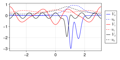
Figure 2. Potentials $V_{j}$ for $j\in\{1,2,3\}$ and the ground states $u_{j}$ of $-\Delta+V_{j}$.

5.2. Eigenvector continuation versus perturbation theory

We define the approximation of $\phi_{\mu}(\lambda)$ given by perturbation theory and the corresponding eigenvalue approximation

$$\varphi_{\mu}(\lambda):=\frac{\sum_{n=0}^{\ell}\lambda^{n}\phi^{n}_{\mu}}{\left|\!\left|\sum_{n=0}^{\ell}\lambda^{n}\phi^{n}_{\mu}\right|\!\right|},\qquad\qquad e_{\mu}(\lambda):=\left<\varphi_{\mu}(\lambda),H(\lambda)\varphi_{\mu}(\lambda)\right>.$$

It is well-known that those quantities coming from perturbation theory respect the following bounds.

Lemma 5.1.

Let us make the definitions and assumptions of Sections 4.1.1 and 4.1.2. By defining $\xi^{\textup{nd,vec}}_{\textup{pert},\ell,\delta}:=\left|\!\left|\phi^{\ell+1}_{\mu}\right|\!\right|_{e,\delta}$ and $\xi^{\textup{nd},E}_{\textup{pert},\ell}:=\left|E^{2(\ell+1)}_{\mu}\right|$, for $\delta\in\{0,1\}$ we have

$$\left|\left|\!\left|\phi_{\mu}(\lambda)-\varphi_{\mu}(\lambda)\right|\!\right|_{e,\delta}-\left|\lambda\right|^{\ell+1}\xi^{\textup{nd,vec}}_{\textup{pert},\ell,\delta}\right| \leqslant c\left(\left|\lambda\right|b\right)^{\ell+2},$$

$$\left|\left|E_{\mu}(\lambda)-e_{\mu}(\lambda)\right|-\left|\lambda\right|^{2(\ell+1)}\xi^{\textup{nd},E}_{\textup{pert},\ell}\right| \leqslant c\left(\left|\lambda\right|b\right)^{2\ell+3},$$

where $b$ and $c$ are independent of $\lambda$ and $\ell$.

A proof is provided in Section 12. The errors given by eigenvector continuation and perturbation theory have the same order in $\left|\lambda\right|$ but have different constants. The relevent quantity enabling to compare eigenvector continuation and perturbation theory in the asymptotic regime is $\xi_{0}:=1$ and for $\ell\geqslant 1$,

$$\xi_{\ell}:=\underset{\begin{subarray}{c}\lambda\rightarrow 0\end{subarray}}{\text{{lim}}}\;\frac{\left|\!\left|\phi_{\mu}(\lambda)-\varphi_{\mu}(\lambda)\right|\!\right|}{\left|\!\left|\phi_{\mu}(\lambda)-\psi_{\mu}(\lambda)\right|\!\right|}=\frac{\xi^{\textup{nd,vec}}_{\textup{pert},\ell,0}}{\xi_{\textup{ec},\ell,0}^{\textup{nd,vec}}}=\frac{\left|\!\left|\phi^{\ell+1}_{\mu}\right|\!\right|}{\left|\!\left|\left(1+R_{\mu}(0)H(0)\right)\mathcal{P}^{\perp}\phi^{\ell+1}_{\mu}\right|\!\right|},$$

but one could also use $\left|\!\left|\left(1+R_{\mu}(0)H(0)\right)\mathcal{P}^{\perp}\phi^{\ell+1}_{\mu}\right|\!\right|_{e}^{-1}\left|\!\left|\phi^{\ell+1}_{\mu}\right|\!\right|_{e}$, which is very close. This quantifies the acceleration that eigenvector continuation provides with respect to perturbation theory. The larger $\xi_{\ell}$ is, the most efficient $\mathcal{P}$ is. We numerically found situations such that $\xi_{\ell}<1$ so eigenvector continuation is not necessarily better than perturbation theory, but in general we observe $\xi_{\ell}>1$.

In our simulations, we will display the errors made by eigenvector continuation (plain lines) and the ones made by perturbation theory (dashed lines), at the level of eigenvectors and eigenvalues.

It is as if the perturbative regime was attained sooner than with perturbation theory

5.3. Varying $\ell$

In this section, we aim at making $\ell$ vary. We choose $\mathcal{P}^{\ell}$ to be the orthogonal projection onto

$$\operatorname{Span}\left(\left(\tfrac{{\rm d}^{n}}{{\rm d}\lambda^{n}}\phi(\lambda)\right)_{\mkern 1.0mu\vrule height=6.02777pt\mkern 2.0mu\lambda=0},0\leqslant n\leqslant\ell\right)$$

where $\phi(\lambda)$ is the eigenvector corresponding to the lowest eigenvalue $E(\lambda)$ of $H(\lambda)$, and we denote by $\psi^{\ell}(\lambda)$ the eigenvector of lowest eigenvalue $\mathcal{E}^{\ell}(\lambda)$ of $\mathcal{P}^{\ell}H(\lambda)\mathcal{P}^{\ell}$. We define the perturbative approximations $\varphi^{\ell}(\lambda):=\frac{\sum_{n=0}^{\ell}\lambda^{n}\phi^{n}}{\left|\!\left|\sum_{n=0}^{\ell}\lambda^{n}\phi^{n}\right|\!\right|}$ and $e^{\ell}(\lambda):=\left<\varphi^{\ell}(\lambda),H(\lambda)\varphi^{\ell}(\lambda)\right>$.

On Figure 3, we plot the errors against $\lambda$ and near $\lambda=0$. The asymptotic slopes correspond to (44) and (45). We see that the perturbation regime (the value of $\lambda$ for which the asymptotic slopes of $\lambda\rightarrow 0$ are followed) for perturbation theory is precisely attained around $\lambda\simeq 1.5$ for all values of $\ell$. On the contrary, in the case of eigenvector continuation, it is not clear where the asymptotic regime starts.

On Table 1 and Figure 4, we display the acceleration constant $\xi_{\ell}$ with respect to $\ell$. We also define $\xi_{\ell}^{\text{simple}}:=\left|\!\left|\mathcal{P}^{\perp}\phi^{\ell+1}_{\mu}\right|\!\right|^{-1}\left|\!\left|\phi^{\ell+1}_{\mu}\right|\!\right|$ to show in Figure 4 that this simpler quantity is close to $\xi_{\ell}$. We see on Figure 4 that the asymptotic behaviors when $\ell\rightarrow+\infty$ are $\xi^{\textup{nd,vec}}_{\textup{pert},\ell}\simeq c_{\text{pert}}s_{\text{pert}}^{\ell}$ and $\xi^{\textup{nd,vec}}_{\textup{ec},\ell}\simeq c_{\text{ec}}s_{\text{ec}}^{\ell}$ with $s_{\text{ec}}<s_{\text{pert}}$. Hence we can conjecture that

$$\left|\!\left|\phi(\lambda)-\varphi^{\ell}(\lambda)\right|\!\right|\simeq r_{\text{pert}}\left(\left|\lambda\right|q_{\text{pert}}\right)^{\ell},\qquad\left|\!\left|\phi(\lambda)-\psi^{\ell}(\lambda)\right|\!\right|\simeq r_{\text{ec}}\left(\left|\lambda\right|q_{\text{ec}}\right)^{\ell}$$

with $q_{\text{ec}}<q_{\text{pert}}$, as if eigenvector continuation had the same error behavior as perturbation theory but where the perturbative regime is attained sooner than for perturbative theory.

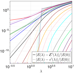
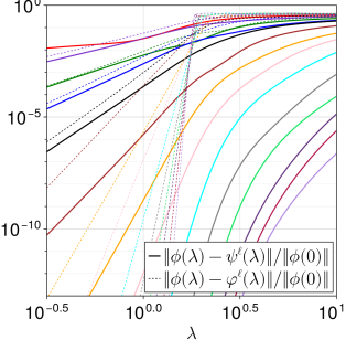
Figure 3. Varying $\ell$, in the case of only one eigenmode. The asymptotic slopes near $0$ are $\ell+1$ on the right and $2\ell+2$ on the left, corresponding to (44) and (45).

$\ell$	0	1	2	3	4	5	6	7	8	9	10	11	12	13
$\xi_{\ell}$	1	1.7	1.3	2.1	6.7	2.4	9.3	10	110	127	37	260	149	899
$\xi^{\text{simple}}_{\ell}$	1	1.7	1.6	2.2	7.8	3.7	12	14	122	178	57	339	203	1242

Table 1. First values of the asymptotic acceleration coefficients against $\ell$, quantifying the advantage of eigenvector continuation with respect to perturbation theory in the perturbative regime.

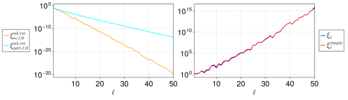
Figure 4. Left: values of $\xi^{\textup{nd,vec}}_{\textup{pert},\ell}$ and $\xi^{\textup{nd,vec}}_{\textup{ec},\ell}$ against $\ell$. Right: acceleration factor $\xi_{\ell}$ against $\ell$. We approximately observe a behavior $\ln_{10}\xi_{\ell}\simeq 0.35\ell$.

6. Proof of Theorem 3.1

We recall that for any self-adjoint operators $B,C$ of $\mathcal{H}$,

$$\left|\!\left|BC\right|\!\right|_{2}\leqslant\left|\!\left|B\right|\!\right|\left|\!\left|C\right|\!\right|_{2}.$$ (54)

Moreover, for any $u,v\in\mathcal{H}$, we have

$$\left|\!\left|\left|u\right>\left<v\right|\right|\!\right|_{2}=\left|\!\left|\left|u\right>\left<v\right|\right|\!\right|=\left|\!\left|u\right|\!\right|\left|\!\left|v\right|\!\right|.$$ (55)

6.1. Decomposition of the error

We decompose the error $\Gamma-\Lambda$ into several terms, which will be possible to handle individually. First, we have $\phi_{\alpha}\in\mathcal{P}\mathcal{H}$, so

$$\mathcal{P}\Lambda=\sum_{\mu=1}^{\nu}\left|\mathcal{P}\phi_{\alpha}\right>\left<\phi_{\alpha}\right|=\sum_{\mu=1}^{\nu}\left|\phi_{\alpha}\right>\left<\phi_{\alpha}\right|=\Lambda,$$

hence

$$\mathcal{P}\Lambda=\Lambda\mathcal{P}=\Lambda,\qquad\qquad\mathcal{P}^{\perp}\Lambda=\Lambda\mathcal{P}^{\perp}=0.$$ (56)

Then we can decompose the error $\Gamma-\Lambda$ in the following way

$$\Gamma-\Lambda \underset{\begin{subarray}{c}1=\mathcal{P}+\mathcal{P}^{\perp}\end{subarray}}{=}\mathcal{P}^{\perp}\left(\Gamma-\Lambda\right)\mathcal{P}^{\perp}+\mathcal{P}\left(\Gamma-\Lambda\right)\mathcal{P}^{\perp}+\mathcal{P}^{\perp}\left(\Gamma-\Lambda\right)\mathcal{P}+\mathcal{P}\left(\Gamma-\Lambda\right)\mathcal{P}$$

$$\underset{\begin{subarray}{c}\eqref{eq:commu}\end{subarray}}{=}\;\mathcal{P}^{\perp}\Gamma\mathcal{P}^{\perp}+\mathcal{P}\Gamma\mathcal{P}^{\perp}+\mathcal{P}^{\perp}\Gamma\mathcal{P}+\mathcal{P}\left(\Gamma-\Lambda\right)\mathcal{P}.$$ (57)

We will follow those steps :

• in Section 6.2 we show how to treat the first terms $\mathcal{P}^{\perp}\Gamma\mathcal{P}^{\perp}$, $\mathcal{P}\Gamma\mathcal{P}^{\perp}$, and $\mathcal{P}^{\perp}\Gamma\mathcal{P}$,

• in Section 6.3 we present a first way of treating the term $\mathcal{P}\left(\Gamma-\Lambda\right)\mathcal{P}$, which will be developed in Sections 6.4, 6.5, 6.6 and 6.7,

• in Section 6.9 we present a second way of treating $\mathcal{P}\left(\Gamma-\Lambda\right)\mathcal{P}$, leading to a different kind of inequalities.

6.2. Treating $\mathcal{P}^{\perp}\Gamma\mathcal{P}^{\perp}$, $\mathcal{P}\Gamma\mathcal{P}^{\perp}$ and $\mathcal{P}^{\perp}\Gamma\mathcal{P}$

We start by treating the first terms of (6.1). We have

$$\left|\!\left|\mathcal{P}^{\perp}\Gamma\mathcal{P}^{\perp}\right|\!\right|_{2,\delta}\underset{\begin{subarray}{c}\Gamma=\Gamma^{2}\end{subarray}}{=}\;\left|\!\left|A^{\delta}\mathcal{P}^{\perp}\Gamma^{2}\mathcal{P}^{\perp}\right|\!\right|_{2}\underset{\begin{subarray}{c}\eqref{eq:bound_norm}\end{subarray}}{\leqslant}\;\left|\!\left|\mathcal{P}^{\perp}\Gamma\right|\!\right|_{2,\delta}\left|\!\left|\mathcal{P}^{\perp}\Gamma\right|\!\right|\\ =\left|\!\left|\mathcal{P}^{\perp}\Gamma\right|\!\right|_{2,\delta}\left|\!\left|A^{-\delta}A^{\delta}\mathcal{P}^{\perp}\Gamma\right|\!\right|\leqslant c_{A}^{\delta}\left|\!\left|\mathcal{P}^{\perp}\Gamma\right|\!\right|_{2,\delta}^{2}.$$

Then,

$$\left|\!\left|A^{\delta}\mathcal{P}^{\perp}\Gamma\mathcal{P}\right|\!\right|_{2}+\left|\!\left|A^{\delta}\mathcal{P}\Gamma\mathcal{P}^{\perp}\right|\!\right|_{2}\leqslant c_{A}^{\delta}\left(\left|\!\left|A^{\delta}\mathcal{P}^{\perp}\Gamma\mathcal{P}A^{\delta}\right|\!\right|_{2}+\left|\!\left|A^{\delta}\mathcal{P}\Gamma\mathcal{P}^{\perp}A^{\delta}\right|\!\right|_{2}\right)$$

$$\qquad=2c_{A}^{\delta}\left|\!\left|A^{\delta}\mathcal{P}^{\perp}\Gamma\mathcal{P}A^{\delta}\right|\!\right|_{2}=2c_{A}^{\delta}\left|\!\left|A^{\delta}\mathcal{P}^{\perp}\Gamma^{2}A^{\delta}A^{-\delta}\mathcal{P}A^{\delta}\right|\!\right|_{2}$$

$$\qquad\leqslant 2c_{A}^{\delta}\left|\!\left|A^{\delta}\mathcal{P}^{\perp}\Gamma\right|\!\right|_{2}\left|\!\left|\Gamma A^{\delta}\right|\!\right|\left|\!\left|A^{-\delta}\mathcal{P}A^{\delta}\right|\!\right|=2\left(c_{A}c_{\mathcal{P}}\left|\!\left|A\Gamma\right|\!\right|\right)^{\delta}\left|\!\left|\mathcal{P}^{\perp}\Gamma\right|\!\right|_{2,\delta}.$$

6.3. A first treatment of $\mathcal{P}\left(\Gamma-\Lambda\right)\mathcal{P}$

We present a first treatment of $\mathcal{P}\left(\Gamma-\Lambda\right)\mathcal{P}$, based on the decomposition $\mathcal{P}=\mathcal{P}(\Lambda+\Lambda^{\perp})=\mathcal{P}\Lambda^{\perp}+\Lambda$. More precisely,

$$\mathcal{P}\left(\Gamma-\Lambda\right)\mathcal{P} =\mathcal{P}\Lambda^{\perp}\left(\Gamma-\Lambda\right)\Lambda+\Lambda\left(\Gamma-\Lambda\right)\mathcal{P}\Lambda^{\perp}$$

$$\qquad\qquad\qquad+\Lambda\left(\Gamma-\Lambda\right)\Lambda+\mathcal{P}\Lambda^{\perp}\left(\Gamma-\Lambda\right)\Lambda^{\perp}\mathcal{P}$$

$$\underset{\begin{subarray}{c}\eqref{eq:commu}\end{subarray}}{=}\;\mathcal{P}\Lambda^{\perp}\Gamma\Lambda+\Lambda\Gamma\mathcal{P}\Lambda^{\perp}+\Lambda\left(\Gamma-\Lambda\right)\Lambda+\mathcal{P}\Lambda^{\perp}\Gamma\Lambda^{\perp}\mathcal{P}.$$ (58)

In the following sections, we provide inequalities for each of those terms.

6.4. Treating $\Lambda\left(\Gamma-\Lambda\right)\Lambda$

On the first hand,

$$\left(\Lambda\left(\Gamma-\Lambda\right)\Lambda\right)^{2}=\left(\Lambda\Gamma\Lambda-\Lambda\right)^{2}=\Lambda\Gamma\Lambda\Gamma\Lambda-2\Lambda\Gamma\Lambda+\Lambda$$

hence

$$\left|\!\left|\Lambda\left(\Gamma-\Lambda\right)\Lambda\right|\!\right|_{2}^{2}=\operatorname{Tr}\left(\Lambda\left(\Gamma-\Lambda\right)\Lambda\right)^{2}=\operatorname{Tr}\Gamma\Lambda\Gamma\Lambda-2\operatorname{Tr}\Gamma\Lambda+\nu.$$

On the other hand,

$$\left(\Gamma-\Lambda\right)^{4} =\left(\Gamma+\Lambda-\Lambda\Gamma-\Gamma\Lambda\right)^{2}$$

$$=\Gamma+\Lambda-\Lambda\Gamma\Lambda-\Gamma\Lambda\Gamma-\Gamma\Lambda-\Lambda\Gamma+\Gamma\Lambda\Gamma\Lambda+\Lambda\Gamma\Lambda\Gamma,$$

so

$$\left|\!\left|\left(\Gamma-\Lambda\right)^{2}\right|\!\right|_{2}^{2}=2\left(\operatorname{Tr}\Gamma\Lambda\Gamma\Lambda-2\operatorname{Tr}\Gamma\Lambda+\nu\right).$$

Then, we see that

$$\left|\!\left|\Lambda\left(\Gamma-\Lambda\right)\Lambda\right|\!\right|_{2}=\frac{1}{\sqrt{2}}\left|\!\left|\left(\Gamma-\Lambda\right)^{2}\right|\!\right|_{2}\leqslant\frac{1}{\sqrt{2}}\left|\!\left|\Gamma-\Lambda\right|\!\right|_{2}^{2}.$$ (59)

Finally,

$$\left|\!\left|\Lambda\left(\Gamma-\Lambda\right)\Lambda\right|\!\right|_{2,\delta} =\left|\!\left|A^{\delta}\Lambda\left(\Gamma-\Lambda\right)\Lambda\right|\!\right|_{2}=\left|\!\left|A^{\delta}\Lambda^{2}\left(\Gamma-\Lambda\right)\Lambda\right|\!\right|_{2}$$

$$\leqslant\left|\!\left|A^{\delta}\Lambda\right|\!\right|\left|\!\left|\Lambda\left(\Gamma-\Lambda\right)\Lambda\right|\!\right|_{2}=\left|\!\left|A\Lambda\right|\!\right|^{\delta}\left|\!\left|\Lambda\left(\Gamma-\Lambda\right)\Lambda\right|\!\right|_{2}$$

$$\underset{\begin{subarray}{c}\eqref{eq:ineq_lambda_gamma_lambda}\end{subarray}}{\leqslant}\;2^{-\frac{1}{2}}\left|\!\left|A\Lambda\right|\!\right|^{\delta}\left|\!\left|\Gamma-\Lambda\right|\!\right|_{2}^{2}\leqslant 2^{-\frac{1}{2}}\left(c_{A}^{2}\left|\!\left|A\Lambda\right|\!\right|\right)^{\delta}\left|\!\left|\Gamma-\Lambda\right|\!\right|_{2,\delta}^{2}$$

$$\leqslant\left(1+c_{A}(1+c_{A})\left|\!\left|A\Lambda\right|\!\right|\right)^{2\delta}\left|\!\left|\Gamma-\Lambda\right|\!\right|_{2}^{2}.$$ (60)

6.5. Treating $\mathcal{P}\Lambda^{\perp}\Gamma\Lambda^{\perp}\mathcal{P}$

We have

$$\left|\!\left|A\mathcal{P}\Lambda^{\perp}A^{-1}\right|\!\right|=\left|\!\left|A\mathcal{P}A^{-1}\left(1-A\Lambda A^{-1}\right)\right|\!\right|\\ \leqslant c_{\mathcal{P}}\left(1+\left|\!\left|A\Lambda A^{-1}\right|\!\right|\right)\leqslant c_{\mathcal{P}}\left(1+c_{A}\left|\!\left|A\Lambda\right|\!\right|\right).$$ (61)

Now, we develop

$$\left|\!\left|\mathcal{P}\Lambda^{\perp}\Gamma\Lambda^{\perp}\mathcal{P}\right|\!\right|_{2,\delta}\leqslant c_{A}^{\delta}\left|\!\left|A^{\delta}\mathcal{P}\Lambda^{\perp}\Gamma^{2}\Lambda^{\perp}\mathcal{P}A^{\delta}\right|\!\right|_{2}\leqslant c_{A}^{\delta}\left|\!\left|A^{\delta}\mathcal{P}\Lambda^{\perp}\Gamma\right|\!\right|_{2}^{2}$$

$$\qquad=c_{A}^{\delta}\left|\!\left|A^{\delta}\mathcal{P}\Lambda^{\perp}\left(\Gamma-\Lambda\right)\right|\!\right|_{2}^{2}=c_{A}^{\delta}\left|\!\left|A^{\delta}\mathcal{P}\Lambda^{\perp}A^{-\delta}A^{\delta}\left(\Gamma-\Lambda\right)\right|\!\right|_{2}^{2}$$

$$\qquad\leqslant c_{A}^{\delta}\left|\!\left|A^{\delta}\mathcal{P}\Lambda^{\perp}A^{-\delta}\right|\!\right|^{2}\left|\!\left|\Gamma-\Lambda\right|\!\right|_{2,\delta}^{2}\leqslant c_{A}^{\delta}\left|\!\left|A\mathcal{P}\Lambda^{\perp}A^{-1}\right|\!\right|^{2\delta}\left|\!\left|\Gamma-\Lambda\right|\!\right|_{2,\delta}^{2}$$

$$\qquad\underset{\begin{subarray}{c}\eqref{eq:bound_APLambdapAiv}\end{subarray}}{\leqslant}\;c_{A}^{\delta}\left(c_{\mathcal{P}}\left(1+c_{A}\left|\!\left|A\Lambda\right|\!\right|\right)\right)^{2\delta}\left|\!\left|\Gamma-\Lambda\right|\!\right|_{2,\delta}^{2}$$

$$\qquad\leqslant\left(c_{A}c_{\mathcal{P}}^{2}\right)^{\delta}\left(1+c_{A}(1+c_{A})\left|\!\left|A\Lambda\right|\!\right|\right)^{2\delta}\left|\!\left|\Gamma-\Lambda\right|\!\right|_{2,\delta}^{2}.$$ (62)

6.6. Definition and properties of partial inverses

To prepare the next section, we need Liouvillian operators, which are standard tools to partially invert Hamiltonians acting on density matrices, see for instance [17, 30, 2, 23] and [7, Section 5.1]. We show several basic equations that will be used.

We define

$$R_{\mu}:=\left(\mathcal{E}_{\mu}-\mathcal{P}H\mathcal{P}\right)^{-1}_{\perp},$$

the super-operators $\mathcal{L}$ and $\mathcal{L}^{+}$ acting on $\mathfrak{S}_{2}$ by

$$B\mapsto\mathcal{L}B:=[\mathcal{P}H\mathcal{P},B],\qquad B\mapsto\mathcal{L}^{+}B:=-\sum_{\mu=1}^{\nu}R_{\mu}BP_{\psi_{\mu}}$$

and the subspaces

$$\mathcal{O}_{1}:=\{B\in\mathfrak{S}_{2},B=\mathcal{P}\Lambda^{\perp}B\mathcal{P}^{\perp}\},\qquad\mathcal{O}_{2}:=\{B\in\mathfrak{S}_{2},B=\mathcal{P}^{\perp}B\mathcal{P}\Lambda^{\perp}\}.$$

By definition of $R_{\mu}$ we have

$$\mathcal{P}\left(\mathcal{E}_{\mu}-H\right)R_{\mu}=\Lambda^{\perp}\mathcal{P}=R_{\mu}\left(\mathcal{E}_{\mu}-H\right)\mathcal{P}.$$ (63)

We compute, for any $B\in\mathfrak{S}_{2}$,

$$\mathcal{L}^{+}\mathcal{L}B =-\sum_{\mu=1}^{\nu}R_{\mu}[\mathcal{P}H\mathcal{P},B]P_{\psi_{\mu}}\underset{\begin{subarray}{c}\mathcal{P}H\mathcal{P}P_{\psi_{\mu}}\\ =\mathcal{E}_{\mu}P_{\psi_{\mu}}\end{subarray}}{=}\;\sum_{\mu=1}^{\nu}\left(\mathcal{E}_{\mu}R_{\mu}BP_{\psi_{\mu}}-R_{\mu}\mathcal{P}H\mathcal{P}BP_{\psi_{\mu}}\right)$$

$$=\sum_{\mu=1}^{\nu}R_{\mu}\left(\mathcal{E}_{\mu}-H\right)\mathcal{P}BP_{\psi_{\mu}}\underset{\begin{subarray}{c}\eqref{eq:KjHE}\end{subarray}}{=}\;\mathcal{P}\Lambda^{\perp}B\sum_{\mu=1}^{\nu}P_{\psi_{\mu}}=\mathcal{P}\Lambda^{\perp}B\Lambda.$$

We can show that $\mathcal{L}^{+}\mathcal{L}$ is the orthogonal projection onto $\mathcal{O}_{1}$. We provide the details here as well for the sake of completeness. For any $B\in\mathfrak{S}_{2}$, we have

$$\mathcal{L}\mathcal{L}^{+}B =\left[\mathcal{P}H\mathcal{P},-\sum_{\mu=1}^{\nu}R_{\mu}BP_{\psi_{\mu}}\right]=\sum_{\mu=1}^{\nu}\left(\mathcal{E}_{\mu}R_{\mu}BP_{\psi_{\mu}}-\mathcal{P}H\mathcal{P}R_{\mu}BP_{\psi_{\mu}}\right)$$

$$=\sum_{\mu=1}^{\nu}\mathcal{P}\left(\mathcal{E}_{\mu}-H\right)R_{\mu}BP_{\psi_{\mu}}=\Lambda^{\perp}\mathcal{P}B\Lambda,$$

hence $\mathcal{L}\mathcal{L}^{+}=\mathcal{L}^{+}\mathcal{L}$. Moreover, for any $F,B\in\mathfrak{S}_{2}$,

$$\left(F,\mathcal{L}^{+}\mathcal{L}B\right)_{\text{2}} =\operatorname{Tr}F^{*}\Lambda^{\perp}\mathcal{P}B\Lambda=\operatorname{Tr}\Lambda F^{*}\Lambda^{\perp}\mathcal{P}B=\operatorname{Tr}\big{(}\mathcal{P}\Lambda^{\perp}F\Lambda\big{)}^{*}B$$

$$=\left(\mathcal{L}^{+}\mathcal{L}F,B\right)_{\text{2}}$$

thus $(\mathcal{L}^{+}\mathcal{L})^{*}=\mathcal{L}^{+}\mathcal{L}$. Finally,

$$\left(\mathcal{L}^{+}\mathcal{L}\right)^{2}B=\left(\mathcal{L}^{+}\mathcal{L}\right)\big{(}\Lambda^{\perp}\mathcal{P}B\Lambda\big{)}=\Lambda^{\perp}\mathcal{P}\big{(}\Lambda^{\perp}\mathcal{P}B\Lambda\big{)}\Lambda=\Lambda^{\perp}\mathcal{P}B\Lambda=\mathcal{L}^{+}\mathcal{L}B,$$

hence $(\mathcal{L}^{+}\mathcal{L})^{2}=\mathcal{L}^{+}\mathcal{L}$, and we can conclude that $\mathcal{L}^{+}\mathcal{L}$ is the orthogonal projection onto $\mathcal{O}_{1}$.

From (56), we have that $\Lambda$ and $\Lambda^{\perp}$ commute with $\mathcal{P}$ and $H$, hence for $Q,G\in\{\Lambda,\mathcal{P}\Lambda^{\perp}\}$ and for any operator $B\in\mathfrak{S}_{2}$,

$$\mathcal{L}\left(QBG\right)=Q\left(\mathcal{L}B\right)G.$$ (64)

6.7. Treating $\mathcal{P}\Lambda^{\perp}\Gamma\Lambda$ and $\Lambda\Gamma\mathcal{P}\Lambda^{\perp}$

We now use the Liouvillian operator to treat $\mathcal{P}\Lambda^{\perp}\Gamma\Lambda$. The Euler-Lagrange equation for $\Gamma$ is $[H,\Gamma]=0$ and can be verified by developping $\Gamma$ into projectors. There holds

$$\mathcal{L}\Gamma =[\mathcal{P}H\mathcal{P},\Gamma]=\mathcal{P}[H,\Gamma]\mathcal{P}-\left(\mathcal{P}H[\mathcal{P}^{\perp},\Gamma]+[\mathcal{P}^{\perp},\Gamma]H\mathcal{P}\right)$$

$$\underset{\begin{subarray}{c}[H,\Gamma]=0\end{subarray}}{=}\;-\mathcal{P}H[\mathcal{P}^{\perp},\Gamma]-[\mathcal{P}^{\perp},\Gamma]H\mathcal{P}.$$ (65)

Next,

$$\mathcal{P}\Lambda^{\perp}\Gamma\Lambda =\mathcal{L}^{+}\mathcal{L}\Gamma\underset{\begin{subarray}{c}\eqref{eq:this_one}\end{subarray}}{=}\;\sum_{\mu=1}^{\nu}R_{\mu}\left(\mathcal{P}H[\mathcal{P}^{\perp},\Gamma]+[\mathcal{P}^{\perp},\Gamma]H\mathcal{P}\right)P_{\psi_{\mu}}$$

$$\underset{\begin{subarray}{c}\mathcal{P}^{\perp}P_{\psi_{\mu}}=0\\ R_{\mu}\mathcal{P}^{\perp}=0\end{subarray}}{=}\;\sum_{\mu=1}^{\nu}R_{\mu}\big{(}H\mathcal{P}^{\perp}\Gamma-\Gamma\mathcal{P}^{\perp}H\big{)}P_{\psi_{\mu}}.$$ (66)

This part is to be associated with $\Lambda^{\perp}$

$$\mathcal{P}^{\perp}\Gamma\mathcal{P}=\mathcal{P}^{\perp}\Gamma\Lambda+\mathcal{P}^{\perp}\Gamma\Lambda^{\perp}\mathcal{P}=\mathcal{P}^{\perp}\Gamma\sum_{\mu=1}^{\nu}P_{\psi_{\mu}}+\mathcal{P}^{\perp}\left(\Gamma-\Lambda\right)^{2}\Lambda^{\perp}\mathcal{P},$$

where we see that the last term is quadratic in $\Gamma-\Lambda$ and hence will be negligible. Thus

$$\mathcal{P}\Lambda^{\perp}\Gamma\Lambda+\mathcal{P}^{\perp}\Gamma\mathcal{P}=\sum_{\mu=1}^{\nu}\left(1+R_{\mu}H\right)H\mathcal{P}^{\perp}\Gamma P_{\psi_{\mu}}\\ -\sum_{\mu=1}^{\nu}R_{\mu}\Gamma\mathcal{P}^{\perp}HP_{\psi_{\mu}}+\mathcal{P}^{\perp}\left(\Gamma-\Lambda\right)^{2}\Lambda^{\perp}\mathcal{P}.$$ (67)

Taking the adjoint operator of (6.7) yields

$$\Lambda\Gamma\mathcal{P}\Lambda^{\perp}=\sum_{\mu=1}^{\nu}P_{\psi_{\mu}}\big{(}\Gamma\mathcal{P}^{\perp}H-H\mathcal{P}^{\perp}\Gamma\big{)}R_{\mu}.$$

As for the bounds, we have

$$\left|\!\left|(1+R_{\mu}H)\mathcal{P}^{\perp}\Gamma P_{\psi_{\mu}}\right|\!\right|_{2,\delta}+\left|\!\left|P_{\psi_{\mu}}\Gamma\mathcal{P}^{\perp}(1+HR_{\mu})\right|\!\right|_{2,\delta}$$

$$\quad=\left|\!\left|A^{\delta}(1+R_{\mu}H)\mathcal{P}^{\perp}\Gamma P_{\psi_{\mu}}\Lambda A^{\delta}A^{-\delta}\right|\!\right|_{2}+\left|\!\left|A^{\delta}\Lambda P_{\psi_{\mu}}\Gamma\mathcal{P}^{\perp}(1+HR_{\mu})A^{\delta}A^{-\delta}\right|\!\right|_{2}$$

$$\quad\leqslant 2c_{A}^{\delta}\left|\!\left|A^{\delta}(1+R_{\mu}H)\mathcal{P}^{\perp}\Gamma P_{\psi_{\mu}}\Lambda A^{\delta}\right|\!\right|_{2}$$

$$\quad=2c_{A}^{\delta}\left|\!\left|A^{\delta}(1+R_{\mu}H)\mathcal{P}^{\perp}A^{-\delta}A^{\delta}\mathcal{P}^{\perp}\Gamma P_{\psi_{\mu}}\Lambda A^{\delta}\right|\!\right|_{2}$$

$$\quad\leqslant 2\left(c_{A}\left|\!\left|A\Lambda\right|\!\right|\right)^{\delta}\left|\!\left|A^{\delta}(1+R_{\mu}H)\mathcal{P}^{\perp}A^{-\delta}\right|\!\right|\left|\!\left|\mathcal{P}^{\perp}\Gamma\right|\!\right|_{2,\delta}.$$ (68)

Similarly,

$$\left|\!\left|R_{\mu}\Gamma\mathcal{P}^{\perp}HP_{\psi_{\mu}}\right|\!\right|_{e,2}+\left|\!\left|P_{\psi_{\mu}}H\mathcal{P}^{\perp}\Gamma R_{\mu}\right|\!\right|_{e,2}\leqslant 2c_{A}^{\delta}\left|\!\left|A^{\delta}R_{\mu}\Gamma\mathcal{P}^{\perp}HP_{\psi_{\mu}}A^{\delta}\right|\!\right|_{2}$$

$$\qquad\underset{\begin{subarray}{c}R_{\mu}\Lambda=0\end{subarray}}{=}\;2c_{A}^{\delta}\left|\!\left|A^{\delta}R_{\mu}\left(\Gamma-\Lambda\right)\Gamma\big{(}\mathcal{P}^{\perp}\big{)}^{2}H\Lambda P_{\psi_{\mu}}\Lambda A^{\delta}\right|\!\right|_{2}$$

$$\qquad\leqslant 2c_{A}^{\delta}\left|\!\left|A^{\delta}R_{\mu}\right|\!\right|\left|\!\left|\Gamma-\Lambda\right|\!\right|\left|\!\left|\Gamma\mathcal{P}^{\perp}\right|\!\right|_{2}\left|\!\left|\mathcal{P}^{\perp}H\Lambda\right|\!\right|\left|\!\left|\Lambda A\right|\!\right|^{\delta}$$

$$\qquad\leqslant 2\left(c_{A}^{2}\left|\!\left|A\Lambda\right|\!\right|\right)^{\delta}\left|\!\left|A^{\delta}R_{\mu}\right|\!\right|\left|\!\left|\Gamma-\Lambda\right|\!\right|\left|\!\left|\mathcal{P}^{\perp}H\Lambda\right|\!\right|\left|\!\left|\mathcal{P}^{\perp}\Gamma\right|\!\right|_{2,\delta}.$$ (69)

Finally,

$$\left|\!\left|\mathcal{P}^{\perp}\Gamma\Lambda^{\perp}\mathcal{P}\right|\!\right|_{2,\delta}+\left|\!\left|\mathcal{P}\Lambda^{\perp}\Gamma\mathcal{P}^{\perp}\right|\!\right|_{2,\delta}\leqslant 2c_{A}^{\delta}\left|\!\left|A^{\delta}\mathcal{P}^{\perp}\Gamma\left(\Gamma-\Lambda\right)\Lambda^{\perp}\mathcal{P}A^{\delta}\right|\!\right|_{2}$$

$$\qquad=2c_{A}^{\delta}\left|\!\left|A^{\delta}\mathcal{P}^{\perp}\Gamma\left(\Gamma-\Lambda\right)A^{\delta}A^{-\delta}\Lambda^{\perp}A^{\delta}A^{-\delta}\mathcal{P}A^{\delta}\right|\!\right|_{2}$$

$$\qquad\leqslant 2\left(c_{A}c_{\mathcal{P}}\left(1+\left|\!\left|A\Lambda\right|\!\right|\right)\right)^{\delta}\left|\!\left|\mathcal{P}^{\perp}\Gamma\right|\!\right|_{2,\delta}\left|\!\left|\Gamma-\Lambda\right|\!\right|_{2,\delta}.$$

6.8. First form

Remark that in this form, gathering all the terms, we have

$$\Gamma-\Lambda=\mathcal{P}^{\perp}\Gamma\mathcal{P}^{\perp}+\mathcal{P}\Gamma\mathcal{P}^{\perp}+\mathcal{P}^{\perp}\Gamma\mathcal{P}+\Lambda\left(\Gamma-\Lambda\right)\Lambda+\mathcal{P}\Lambda^{\perp}\Gamma\Lambda^{\perp}\mathcal{P}\\ +\sum_{\mu=1}^{\nu}\left(P_{\psi_{\mu}}\big{(}\Gamma\mathcal{P}^{\perp}H-H\mathcal{P}^{\perp}\Gamma\big{)}R_{\mu}-R_{\mu}\big{(}\Gamma\mathcal{P}^{\perp}H-H\mathcal{P}^{\perp}\Gamma\big{)}P_{\psi_{\mu}}\right).$$

Now using (67) to associate $\mathcal{P}^{\perp}\Gamma\mathcal{P}$ with $\mathcal{P}\Lambda\Gamma\Lambda$, we obtain (9) where

$$\Omega=\mathcal{P}^{\perp}\left(\Gamma-\Lambda\right)^{2}\mathcal{P}^{\perp}+\Lambda\left(\Gamma-\Lambda\right)\Lambda+\left(\mathcal{P}^{\perp}\left(\Gamma-\Lambda\right)^{2}\Lambda^{\perp}\mathcal{P}+\text{s.a}\right)\\ +\mathcal{P}\Lambda^{\perp}\left(\Gamma-\Lambda\right)^{2}\Lambda^{\perp}\mathcal{P}-\sum_{\mu=1}^{\nu}\left(R_{\mu}\left(\Gamma-\Lambda\right)^{2}\mathcal{P}^{\perp}HP_{\psi_{\mu}}+\textup{s.a}\right).$$ (70)

From (59) we know that $\Lambda\left(\Gamma-\Lambda\right)\Lambda$ is quadratic in $\Gamma-\Lambda$. Hence, we immediately see with this form (9) that when $\Gamma-\Lambda$ is small, the leading term is $\sum_{\mu=1}^{\nu}\left((1+HR_{\mu})\mathcal{P}^{\perp}\Gamma P_{\psi_{\mu}}+\text{s.a}\right)$, and $\Omega$ is quadratic in $\Gamma-\Lambda$, and thus much smaller.

We obtain (10) from the developed inequalities.

6.9. Second form

In this section we present another way of treating $\Gamma-\Lambda$.

For any $z\in\mathbb{C}\backslash\sigma\big{(}(\mathcal{P}H\mathcal{P})_{\mkern 1.0mu\vrule height=6.02777pt\mkern 2.0mu\mathcal{P}\mathcal{H}\rightarrow\mathcal{P}\mathcal{H}}\big{)}$, we define the partial inverse

$$\left(z-\mathcal{P}H\mathcal{P}\right)^{-1}_{\mathcal{P}\mathcal{H}}:=\left\{\begin{array}[]{ll}\left(\left(z-\mathcal{P}H\mathcal{P}\right)_{\mkern 1.0mu\vrule height=6.02777pt\mkern 2.0mu\mathcal{P}\mathcal{H}\rightarrow\mathcal{P}\mathcal{H}}\right)^{-1}&\mbox{on }\mathcal{P}\mathcal{H},\\ 0&\mbox{on }\mathcal{P}^{\perp}\mathcal{H},\end{array}\right.$$ (73)

extended by linearity on $\mathcal{H}$. By the definition (73),

$$\left(z-\mathcal{P}H\mathcal{P}\right)\left(z-\mathcal{P}H\mathcal{P}\right)^{-1}_{\mathcal{P}\mathcal{H}}\varphi=\left\{\begin{array}[]{ll}\varphi&\mbox{if }\varphi\in\mathcal{P}\mathcal{H},\\ 0&\mbox{if }\varphi\in\mathcal{P}^{\perp}\mathcal{H},\end{array}\right.$$

hence

$$\left(z-\mathcal{P}H\mathcal{P}\right)\left(z-\mathcal{P}H\mathcal{P}\right)^{-1}_{\mathcal{P}\mathcal{H}}=\mathcal{P}.$$ (74)

Then

$$\mathcal{P}(z-H)^{-1}\mathcal{P}-(z-\mathcal{P}H\mathcal{P})^{-1}_{\mathcal{P}\mathcal{H}}=\mathcal{P}(z-H)^{-1}\left(\mathcal{P}-(z-H)(z-\mathcal{P}H\mathcal{P})^{-1}_{\mathcal{P}\mathcal{H}}\right)$$

$$\qquad\qquad=\mathcal{P}(z-H)^{-1}\left(\mathcal{P}-(z-\mathcal{P}H\mathcal{P}+\mathcal{P}H\mathcal{P}-H)(z-\mathcal{P}H\mathcal{P})^{-1}_{\mathcal{P}\mathcal{H}}\right)$$

$$\qquad\qquad\underset{\begin{subarray}{c}\eqref{eq:res_PHP}\end{subarray}}{=}\;\mathcal{P}(z-H)^{-1}(H-\mathcal{P}H\mathcal{P})(z-\mathcal{P}H\mathcal{P})^{-1}_{\mathcal{P}\mathcal{H}}$$

$$\qquad\qquad=\mathcal{P}(z-H)^{-1}\mathcal{P}^{\perp}H(z-\mathcal{P}H\mathcal{P})^{-1}_{\mathcal{P}\mathcal{H}},$$

where we used that $(z-\mathcal{P}H\mathcal{P})^{-1}_{\mathcal{P}\mathcal{H}}=\mathcal{P}(z-\mathcal{P}H\mathcal{P})^{-1}_{\mathcal{P}\mathcal{H}}$ in the last step. We now use that

$$\Gamma(z-H)^{-1}=\sum_{\mu=1}^{\nu}P_{\phi_{\mu}}(z-H)^{-1}=\sum_{\mu=1}^{\nu}P_{\phi_{\mu}}(z-H)^{-1}=\sum_{\mu=1}^{\nu}P_{\phi_{\mu}}(z-E_{\mu})^{-1}$$

to deduce $\Gamma(z-H)^{-1}\Gamma^{\perp}=\Gamma^{\perp}(z-H)^{-1}\Gamma=0$ and $\Gamma(z-H)^{-1}=\Gamma(z-H)^{-1}\Gamma$, so we can write

$$(z-H)^{-1}$$

$$\qquad=\Gamma(z-H)^{-1}\Gamma+\Gamma^{\perp}(z-H)^{-1}\Gamma+\Gamma(z-H)^{-1}\Gamma^{\perp}+\Gamma^{\perp}(z-H)^{-1}\Gamma^{\perp}$$

$$\qquad=(z-H)^{-1}_{\perp}+\sum_{\mu=1}^{\nu}P_{\phi_{\mu}}(z-E_{\mu})^{-1}.$$

Similarly,

$$(z-\mathcal{P}H\mathcal{P})^{-1}_{\mathcal{P}\mathcal{H}} =\Lambda(z-\mathcal{P}H\mathcal{P})^{-1}_{\mathcal{P}\mathcal{H}}+\Lambda^{\perp}(z-\mathcal{P}H\mathcal{P})^{-1}_{\mathcal{P}\mathcal{H}}\Lambda^{\perp}$$

$$=(z-\mathcal{P}H\mathcal{P})^{-1}_{\perp}+\sum_{\mu=1}^{\nu}P_{\psi_{\mu}}(z-\mathcal{E}_{\mu})^{-1}.$$

The operators $(z-H)^{-1}_{\perp}$ and $(z-\mathcal{P}H\mathcal{P})^{-1}_{\perp}$ are holomorphic in the interior of $\mathcal{C}$ so they will “participate passively” to the Cauchy integral. Moreover,

$$\frac{1}{2\pi i}\oint_{\mathcal{C}}(z-E_{\mu})^{-1}(z-\mathcal{E}_{\alpha})^{-1}{\rm d}z=\delta_{E_{\mu}\neq\mathcal{E}_{\alpha}}\left((\mathcal{E}_{\alpha}-E_{\mu})^{-1}+(E_{\mu}-\mathcal{E}_{\alpha})^{-1}\right)=0.$$ (75)

We are ready to compute

$$\mathcal{P}\left(\Gamma-\Lambda\right)\mathcal{P}=\frac{1}{2\pi i}\oint_{\mathcal{C}}\left(\mathcal{P}(z-H)^{-1}\mathcal{P}-(z-\mathcal{P}H\mathcal{P})^{-1}_{\mathcal{P}\mathcal{H}}\right){\rm d}z$$

$$\qquad=\frac{1}{2\pi i}\oint_{\mathcal{C}}\mathcal{P}(z-H)^{-1}\mathcal{P}^{\perp}H(z-\mathcal{P}H\mathcal{P})^{-1}_{\mathcal{P}\mathcal{H}}{\rm d}z$$

$$\qquad=\sum_{\mu=1}^{\nu}\left(\mathcal{P}P_{\phi_{\mu}}\mathcal{P}^{\perp}H\left(E_{\mu}-\mathcal{P}H\mathcal{P}\right)_{\perp}^{-1}+\mathcal{P}\left(\mathcal{E}_{\mu}-H\right)_{\perp}^{-1}\mathcal{P}^{\perp}HP_{\psi_{\mu}}\right).$$

As for inequalities, we have

$$\left|\!\left|A^{\delta}\mathcal{P}P_{\phi_{\mu}}\mathcal{P}^{\perp}H\left(E_{\mu}-\mathcal{P}H\mathcal{P}\right)_{\perp}^{-1}\right|\!\right|_{2}$$

$$\qquad=\left|\!\left|A^{\delta}\mathcal{P}A^{-\delta}A^{\delta}\Gamma P_{\phi_{\mu}}\Gamma\mathcal{P}^{\perp}\mathcal{P}^{\perp}H\left(E_{\mu}-\mathcal{P}H\mathcal{P}\right)_{\perp}^{-1}\right|\!\right|_{2}$$

$$\qquad\leqslant\left|\!\left|A^{\delta}\mathcal{P}A^{-\delta}\right|\!\right|\left|\!\left|A^{\delta}\Gamma\right|\!\right|\left|\!\left|P_{\phi_{\mu}}\right|\!\right|_{2}\left|\!\left|\Gamma\mathcal{P}^{\perp}\right|\!\right|\left|\!\left|\mathcal{P}^{\perp}H\left(E_{\mu}-\mathcal{P}H\mathcal{P}\right)_{\perp}^{-1}\right|\!\right|$$

$$\qquad\leqslant\left(c_{A}c_{\mathcal{P}}\left|\!\left|A\Gamma\right|\!\right|\right)^{\delta}\left|\!\left|\left(E_{\mu}-\mathcal{P}H\mathcal{P}\right)_{\perp}^{-1}H\mathcal{P}^{\perp}\right|\!\right|\left|\!\left|\mathcal{P}^{\perp}\Gamma\right|\!\right|_{2,\delta},$$

and

$$\left|\!\left|A^{\delta}\mathcal{P}\left(\mathcal{E}_{\mu}-H\right)_{\perp}^{-1}\mathcal{P}^{\perp}HP_{\psi_{\mu}}\right|\!\right|_{2}=\left|\!\left|A^{\delta}\mathcal{P}A^{-\delta}A^{\delta}\left(\mathcal{E}_{\mu}-H\right)_{\perp}^{-1}\mathcal{P}^{\perp}H\Lambda P_{\psi_{\mu}}\right|\!\right|_{2}$$

$$\qquad\leqslant\left|\!\left|A^{\delta}\mathcal{P}A^{-\delta}\right|\!\right|\left|\!\left|A^{\delta}\left(\mathcal{E}_{\mu}-H\right)_{\perp}^{-1}\right|\!\right|\left|\!\left|\mathcal{P}^{\perp}H\Lambda\right|\!\right|\left|\!\left|P_{\psi_{\mu}}\right|\!\right|_{2}$$

$$\qquad\leqslant c_{\mathcal{P}}^{\delta}\left|\!\left|A^{\delta}\left(\mathcal{E}_{\mu}-H\right)_{\perp}^{-1}\right|\!\right|\left|\!\left|\mathcal{P}^{\perp}H\Lambda\right|\!\right|,$$

and also using the inequalities of Section 6.2, we can deduce (15) of Proposition 3.2.

7. Proof of Proposition 3.3

We now treat the vector case and aim at showing (16) and (17).

7.1. Equality on eigenvectors

Let us keep $\nu\in\mathbb{N}$ general first, we will assume $\nu=1$ later.

Lemma 7.1.

Given the setting of Proposition 3.3, for any $\mu\in\{1,\dots,\nu\}$, assuming that $\left<\phi_{\mu},\psi_{\mu}\right>\in\mathbb{R}$, there holds

$$\big{(}\Lambda^{\perp}+P_{\psi_{\mu}}\big{)}\left(\phi_{\mu}-\psi_{\mu}\right)=\left(1+R_{\mu}H\right)\mathcal{P}^{\perp}\phi_{\mu}\\ -\frac{1}{2}\left|\!\left|\phi_{\mu}-\psi_{\mu}\right|\!\right|^{2}\psi_{\mu}+\left(\mathcal{E}_{\mu}-E_{\mu}\right)R_{\mu}\left(\phi_{\mu}-\psi_{\mu}\right).$$ (76)

The remaining component of $\phi_{\mu}-\psi_{\mu}$ which is not taken into account in this lemma is $\Lambda P_{\psi_{\mu}}^{\perp}(\phi_{\mu}-\psi_{\mu})$.

Proof.

We have $\left(H-E_{\mu}\right)\phi_{\mu}=0$ and $\mathcal{P}\left(H-\mathcal{E}_{\mu}\right)\psi_{\mu}=0$, thus

$$\mathcal{P}\left(H-\mathcal{E}_{\mu}\right)\left(\phi_{\mu}-\psi_{\mu}\right)=\left(E_{\mu}-\mathcal{E}_{\mu}\right)\mathcal{P}\phi_{\mu}.$$ (77)

We first use $[\mathcal{P}H\mathcal{P},\Lambda]=0$, hence $\mathcal{P}H\mathcal{P}\Lambda^{\perp}=\Lambda^{\perp}\mathcal{P}H\mathcal{P}$ and applying $\Lambda^{\perp}$ on the left we obtain $\Lambda^{\perp}\mathcal{P}H\mathcal{P}\Lambda^{\perp}=\Lambda^{\perp}\mathcal{P}H\mathcal{P}$, so

$$\mathcal{P}\Lambda^{\perp}\left(\mathcal{E}_{\mu}-H\right)\Lambda^{\perp}\mathcal{P}\left(\phi_{\mu}-\psi_{\mu}\right)=\mathcal{P}\Lambda^{\perp}\left(\mathcal{E}_{\mu}-H\right)\mathcal{P}\left(\phi_{\mu}-\psi_{\mu}\right)$$

$$\qquad=\Lambda^{\perp}\mathcal{P}\left(\mathcal{E}_{\mu}-H\right)\left(\phi_{\mu}-\psi_{\mu}\right)-\Lambda^{\perp}\mathcal{P}\left(\mathcal{E}_{\mu}-H\right)\mathcal{P}^{\perp}\left(\phi_{\mu}-\psi_{\mu}\right)$$

$$\qquad\underset{\begin{subarray}{c}\eqref{eq:funda}\end{subarray}}{=}\;\left(\mathcal{E}_{\mu}-E_{\mu}\right)\Lambda^{\perp}\mathcal{P}\phi_{\mu}+\Lambda^{\perp}\mathcal{P}H\mathcal{P}^{\perp}\phi_{\mu}.$$

We apply $R_{\mu}$ and use (63), $R_{\mu}\Lambda^{\perp}\mathcal{P}=R_{\mu}$ and $R_{\mu}\psi_{\mu}=0$ to obtain

$$\mathcal{P}\Lambda^{\perp}\left(\phi_{\mu}-\psi_{\mu}\right)=R_{\mu}H\mathcal{P}^{\perp}\phi_{\mu}+\left(\mathcal{E}_{\mu}-E_{\mu}\right)R_{\mu}\left(\phi_{\mu}-\psi_{\mu}\right).$$ (78)

Moreover, in a gauge where $\left<\psi_{\mu},\phi_{\mu}\right>\in\mathbb{R}$,

$$\left<\psi_{\mu},\phi_{\mu}\right>=1-\frac{1}{2}\left|\!\left|\phi_{\mu}-\psi_{\mu}\right|\!\right|^{2}$$

hence

$$P_{\psi_{\mu}}\left(\phi_{\mu}-\psi_{\mu}\right)=\big{(}\left<\psi_{\mu},\phi_{\mu}\right>-1\big{)}\psi_{\mu}=-\frac{1}{2}\left|\!\left|\phi_{\mu}-\psi_{\mu}\right|\!\right|^{2}\psi_{\mu}.$$ (79)

Finally, $\Lambda^{\perp}+P_{\psi_{\mu}}=\mathcal{P}^{\perp}+\mathcal{P}\Lambda^{\perp}+P_{\psi_{\mu}}$ and we obtain (76) by summing (78) and (79) with $\mathcal{P}^{\perp}\left(\phi_{\mu}-\psi_{\mu}\right)=\mathcal{P}^{\perp}\phi_{\mu}$. ∎

We obtain (16) by applying this lemma to $\nu=1$, in which case $\Lambda^{\perp}+P_{\psi_{\mu}}=1$. For $\nu\geqslant 2$, this methods with vectors does not enable to obtain a bound on the remaining component $\Lambda P_{\psi_{\mu}}^{\perp}$, that is why the previous density matrix approach is useful.

7.2. Equality on eigenvalues

Let us first present a well-known and basic estimate showing that the errors between eigenvalues can be expressed as the square of the error between eigenvectors. We give a proof for the sake of completeness.

Lemma 7.2 (Eigenvalue error is quadratic in eigenvector error).

Take two self-adjoint operators $A$ and $H$, assume that $\left|\!\left|A^{-1}\right|\!\right|<+\infty$ and $c_{H}:=\left|\!\left|A^{-1}HA^{-1}\right|\!\right|<+\infty$. Take $\psi$ in the form domain of $H$ and $\phi$ in the domain of $H$, such that $H\phi=E\phi$, $\left|\!\left|\psi\right|\!\right|=\left|\!\left|\phi\right|\!\right|=1$, and define $\mathcal{E}:=\left<\psi,H\psi\right>$. Then

$$E-\mathcal{E} =\left<\phi-\psi,(E-H)\left(\phi-\psi\right)\right>,$$ (80)

$$\left|E-\mathcal{E}\right| \leqslant\left|\!\left|A^{-1}(H-E)A^{-1}\right|\!\right|\underset{\begin{subarray}{c}\theta\in[0,2\pi[\end{subarray}}{\text{{min}}}\;\left|\!\left|A(\phi-e^{i\theta}\psi)\right|\!\right|^{2}.$$ (81)

Usually the bound (81) is used as

$$\left|E-\mathcal{E}\right|\leqslant\left(\left|\!\left|A^{-1}\right|\!\right|^{2}\left|E\right|+\left|\!\left|A^{-1}HA^{-1}\right|\!\right|\right)\underset{\begin{subarray}{c}\theta\in[0,2\pi[\end{subarray}}{\text{{min}}}\;\left|\!\left|A(\phi-e^{i\theta}\psi)\right|\!\right|^{2}.$$

Proof.

By using $(E-H)\phi=0$ and $\left|\!\left|\psi\right|\!\right|=1$, we have

$$\left<\phi-\psi,(E-H)\left(\phi-\psi\right)\right>=-\left<\phi-\psi,(E-H)\psi\right>\\ =-\left<(E-H)\left(\phi-\psi\right),\psi\right>=\left<(E-H)\psi,\psi\right>=E-\left<\psi,H\psi\right>=E-\mathcal{E}.$$

Then

$$\left|E-\mathcal{E}\right| =\left|\left<A(\phi-\psi),A^{-1}(E-H)A^{-1}A\left(\phi-\psi\right)\right>\right|$$

$$\leqslant\left|\!\left|A^{-1}(E-H)A^{-1}\right|\!\right|\left|\!\left|A(\phi-\psi)\right|\!\right|^{2}.$$

To conclude, we change $\psi\rightarrow e^{i\theta}\psi$. ∎

We now have $\nu=1$ and remove the subscript $1$ everywhere. Let us now show (17). First,

$$R\left(H-\mathcal{E}\right)\left(1+RH\right)\mathcal{P}^{\perp}=R(H-\mathcal{E})\mathcal{P}^{\perp}+R\left(H-\mathcal{E}\right)RH\mathcal{P}^{\perp}\\ \underset{\begin{subarray}{c}R\mathcal{P}^{\perp}=0\end{subarray}}{=}\;RH\mathcal{P}^{\perp}+R\left(H-\mathcal{E}\right)\mathcal{P}RH\mathcal{P}^{\perp}\\ \underset{\begin{subarray}{c}R(\mathcal{E}-H)\mathcal{P}=\mathcal{P}P_{\psi}^{\perp}\end{subarray}}{=}\;RH\mathcal{P}^{\perp}-\mathcal{P}P_{\psi}^{\perp}RH\mathcal{P}^{\perp}\underset{\begin{subarray}{c}\mathcal{P}P_{\psi}^{\perp}R=R\end{subarray}}{=}\;0.$$ (82)

Moreover, using (16) we have

$$\left(\mathcal{E}-H\right)\left(\phi-\psi\right)\underset{\begin{subarray}{c}(\mathcal{P}H-\mathcal{E})\psi=0\end{subarray}}{=}\;\left(\mathcal{E}-H\right)\left(\left(1+RH\right)\mathcal{P}^{\perp}\phi+\left(\mathcal{E}-E\right)R\phi\right)$$

$$\qquad\qquad\qquad\qquad\qquad\qquad\qquad\qquad\qquad+\tfrac{1}{2}\left|\!\left|\phi-\psi\right|\!\right|^{2}\mathcal{P}^{\perp}H\psi$$

$$=\left(\mathcal{E}-H\right)\left(1+RH\right)\mathcal{P}^{\perp}\phi+\left(\mathcal{E}-E\right)\mathcal{P}\left(\mathcal{E}-H\right)R\phi$$

$$\qquad\qquad\qquad\qquad\qquad+\left(\mathcal{E}-E\right)\mathcal{P}^{\perp}\left(\mathcal{E}-H\right)R\phi+\tfrac{1}{2}\left|\!\left|\phi-\psi\right|\!\right|^{2}\mathcal{P}^{\perp}H\psi$$

$$=\left(\mathcal{E}-H\right)\left(1+RH\right)\mathcal{P}^{\perp}\phi+\left(\mathcal{E}-E\right)\mathcal{P}P_{\psi}^{\perp}\phi+\left(E-\mathcal{E}\right)\mathcal{P}^{\perp}HR\phi$$

$$\qquad\qquad\qquad\qquad\qquad\qquad\qquad\qquad\qquad+\tfrac{1}{2}\left|\!\left|\phi-\psi\right|\!\right|^{2}\mathcal{P}^{\perp}H\psi.$$ (83)

Similarly as in (80), using $(E-H)\phi=0$ and $\left|\!\left|\psi\right|\!\right|=1$, we have

$$\qquad E-\mathcal{E}=\left<\phi-\psi,(E-H)\left(\phi-\psi\right)\right>$$

$$=\left<\phi-\psi,(\mathcal{E}-H)\left(\phi-\psi\right)\right>+(E-\mathcal{E})\left|\!\left|\phi-\psi\right|\!\right|^{2}$$

$$\underset{\begin{subarray}{c}\eqref{eq:equality_diff}\end{subarray}}{=}\;\left<\left(1+RH\right)\mathcal{P}^{\perp}\phi,\left(\mathcal{E}-H\right)\left(\phi-\psi\right)\right>-\tfrac{1}{2}\left|\!\left|\phi-\psi\right|\!\right|^{2}\left<\psi,\left(\mathcal{E}-H\right)\left(\phi-\psi\right)\right>$$

$$\qquad+\left(\mathcal{E}-E\right)\left<R\phi,\left(\mathcal{E}-H\right)\left(\phi-\psi\right)\right>+(E-\mathcal{E})\left|\!\left|\phi-\psi\right|\!\right|^{2}.$$ (84)

We now compute each of those terms. First, by (7.2) we have

$$\left<\left(1+RH\right)\mathcal{P}^{\perp}\phi,(\mathcal{E}-H)(\phi-\psi)\right>\\ =\left<\left(1+RH\right)\mathcal{P}^{\perp}\phi,\left(\mathcal{E}-H\right)\left(1+RH\right)\mathcal{P}^{\perp}\phi\right>\\ +(\mathcal{E}-E)\left<\left(1+RH\right)\mathcal{P}^{\perp}\phi,\mathcal{P}P_{\psi}^{\perp}\phi\right>+(E-\mathcal{E})\left<\left(1+RH\right)\mathcal{P}^{\perp}\phi,\mathcal{P}^{\perp}HR\phi\right>\\ +\tfrac{1}{2}\left|\!\left|\phi-\psi\right|\!\right|^{2}\left<\left(1+RH\right)\mathcal{P}^{\perp}\phi,\mathcal{P}^{\perp}H\psi\right>.$$

Then using $R\mathcal{P}^{\perp}=0$ and (82), we get

$$\left<\left(1+RH\right)\mathcal{P}^{\perp}\phi,(\mathcal{E}-H)(\phi-\psi)\right>=\left<\mathcal{P}^{\perp}\phi,\left(\mathcal{E}-H\right)\left(1+RH\right)\mathcal{P}^{\perp}\phi\right>\\ +(\mathcal{E}-E)\left<RH\mathcal{P}^{\perp}\phi,\mathcal{P}P_{\psi}^{\perp}\phi\right>+(E-\mathcal{E})\left<\mathcal{P}^{\perp}\phi,\mathcal{P}^{\perp}HR\phi\right>\\ +\tfrac{1}{2}\left|\!\left|\phi-\psi\right|\!\right|^{2}\left<\mathcal{P}^{\perp}\phi,\mathcal{P}^{\perp}H\psi\right>\\ \underset{\begin{subarray}{c}P_{\psi}^{\perp}\mathcal{P}R=R\end{subarray}}{=}\;\left<\mathcal{P}^{\perp}\phi,\left(\mathcal{E}-H\right)\left(1+RH\right)\mathcal{P}^{\perp}\phi\right>+\tfrac{1}{2}\left|\!\left|\phi-\psi\right|\!\right|^{2}\left<\mathcal{P}^{\perp}\phi,H\psi\right>,$$

giving the first term of (7.2). Using (7.2), the second term of (7.2) comes from

$$\left<\psi,(\mathcal{E}-H)(\phi-\psi)\right>=\left<\mathcal{P}\psi,\left(\mathcal{E}-H\right)\left(1+RH\right)\mathcal{P}^{\perp}\phi\right>\\ =\left<\mathcal{P}\psi,(\mathcal{E}-H)\mathcal{P}^{\perp}\phi\right>+\left<\mathcal{P}\psi,(\mathcal{E}-H)RH\mathcal{P}^{\perp}\phi\right>\underset{\begin{subarray}{c}\mathcal{P}(\mathcal{E}-H)R\\ =P_{\psi}^{\perp}\mathcal{P}\end{subarray}}{=}\;-\left<H\psi,\mathcal{P}^{\perp}\phi\right>.$$

The third term of (7.2) comes from

$$\left<R\phi,\left(\mathcal{E}-H\right)\left(\phi-\psi\right)\right>\underset{\begin{subarray}{c}\eqref{eq:interm_eq},\eqref{eq:intermios}\\ R\mathcal{P}^{\perp}=0\end{subarray}}{=}\;\left<R\phi,\left(\mathcal{E}-E\right)\mathcal{P}P_{\psi}^{\perp}\phi\right>\\ \underset{\begin{subarray}{c}R\mathcal{P}P_{\psi}^{\perp}=R\end{subarray}}{=}\;\left(\mathcal{E}-E\right)\left<\phi,R\phi\right>\underset{\begin{subarray}{c}R\psi=0\end{subarray}}{=}\;\left(\mathcal{E}-E\right)\left<\phi-\psi,R\left(\phi-\psi\right)\right>.$$

Summing all the terms of (7.2) yields

$$E-\mathcal{E}=\left<\mathcal{P}^{\perp}\phi,\left(\mathcal{E}-H\right)\left(1+RH\right)\mathcal{P}^{\perp}\phi\right>+\left(E-\mathcal{E}\right)^{2}\left<\phi-\psi,R\left(\phi-\psi\right)\right>\\ +(E-\mathcal{E})\left|\!\left|\phi-\psi\right|\!\right|^{2}+\left|\!\left|\phi-\psi\right|\!\right|^{2}\operatorname{Re}\left<\mathcal{P}^{\perp}\phi,H\psi\right>.$$

Moreover, $\big{(}(\mathcal{E}-H)(1+RH)\big{)}^{*}=(1+HR)(\mathcal{E}-H)=(\mathcal{E}-H)(1+RH)$ is self-adjoint so $\left<\mathcal{P}^{\perp}\phi,\left(\mathcal{E}-H\right)\left(1+RH\right)\mathcal{P}^{\perp}\phi\right>\in\mathbb{R}$, $\left<\phi-\psi,R\left(\phi-\psi\right)\right>\in\mathbb{R}$. To conclude, we use that $\left<\mathcal{P}^{\perp}\phi,H\psi\right>=-\left<\mathcal{P}^{\perp}\phi,(H-E)(\phi-\psi)\right>$.

7.3. Inequalities (21) and (22)

From (16) we have

$$\left|\!\left|\phi-\psi\right|\!\right|_{e}\leqslant\left|\!\left|A\left(1+RH\right)\mathcal{P}^{\perp}\phi\right|\!\right|+\frac{1}{2}\left|\!\left|\phi-\psi\right|\!\right|^{2}\left|\!\left|\psi\right|\!\right|_{e}+\left|\mathcal{E}-E\right|\left|\!\left|AR\left(\phi-\psi\right)\right|\!\right|$$

$$\leqslant\left|\!\left|\left(1+ARAA^{-1}HA^{-1}\right)A\mathcal{P}^{\perp}\phi\right|\!\right|+\frac{1}{2}c_{A}\left|\!\left|\phi-\psi\right|\!\right|\left|\!\left|\phi-\psi\right|\!\right|_{e}\left|\!\left|\psi\right|\!\right|_{e}$$

$$\qquad\qquad\qquad\qquad+\left|\!\left|AR\right|\!\right|\left|\mathcal{E}-E\right|\left|\!\left|\phi-\psi\right|\!\right|$$

$$\leqslant\left(1+\left|\!\left|ARA\right|\!\right|c_{H}\right)\left|\!\left|\mathcal{P}^{\perp}\phi\right|\!\right|_{e}+c_{A}\left(\frac{1}{2}\left|\!\left|\phi-\psi\right|\!\right|\left|\!\left|\psi\right|\!\right|_{e}+\left|\!\left|AR\right|\!\right|\left|\mathcal{E}-E\right|\right)\left|\!\left|\phi-\psi\right|\!\right|_{e},$$

and we obtain (21) when

$$c_{A}\left(\frac{1}{2}\left|\!\left|\phi-\psi\right|\!\right|\left|\!\left|\psi\right|\!\right|_{e}+\left|\!\left|AR\right|\!\right|\left|\mathcal{E}-E\right|\right)\leqslant\frac{1}{2}.$$

Proving (22) uses (80).

We can obtain (18) with the same method, which also needs to use (6.7).

8. Bounds on the Rayleigh-Schrödinger series
in perturbation theory

In the proofs of the theorems of Section 4, we will need some general results about perturbation theory, which we show here. The main results are Lemma 8.3 and Lemma 8.5 on the boundedness of the Rayleigh-Schrödinger series $E^{n}_{\mu}$ and $\phi^{n}_{\mu}$.

We take the context of an analytic and self-adjoint operator family $H(\lambda)$, presented in Section 4.1. In particular, we consider a series of operators

$$H(\lambda)=\sum_{n=0}^{+\infty}\lambda^{n}H^{n},$$

and a cluster of eigenmodes $\left(E_{\mu}(\lambda),\phi_{\mu}(\lambda)\right)_{\mu=1}^{\nu}$ of $H(\lambda)$, where all those maps are analytic in $\lambda\in]-\lambda_{0},\lambda_{0}[$. We define respectively an energy norm and a parameter norm, for any operator $B$ of $\mathcal{H}$, by respectively

$$\left|\!\left|B\right|\!\right|_{2,ee}:=\left|\!\left|ABA\right|\!\right|_{2},\qquad\qquad\left|\!\left|B\right|\!\right|_{p}:=\left|\!\left|A^{-1}BA^{-1}\right|\!\right|.$$

We have $\left|\!\left|B\right|\!\right|_{2,1}\leqslant\left|\!\left|A^{-1}\right|\!\right|\left|\!\left|B\right|\!\right|_{2,ee}$, so the energy norm $\left|\!\left|\cdot\right|\!\right|_{2,ee}$ controls the energy norm $\left|\!\left|\cdot\right|\!\right|_{2,1}$, defined in (2). We use intermediate normalization, which is reviewed in Section A. We set

$$\Phi_{\mu}(\lambda):=\frac{\phi_{\mu}(\lambda)}{\left<\phi_{\mu}^{0},\phi_{\mu}(\lambda)\right>},\qquad\phi_{\mu}^{n}:=\frac{1}{n!}\left(\frac{{\rm d}^{n}}{{\rm d}\lambda^{n}}\phi_{\mu}(\lambda)\right)_{\mkern 1.0mu\vrule height=6.02777pt\mkern 2.0mu\lambda=0},\\ \Phi_{\mu}^{n}:=\frac{1}{n!}\left(\frac{{\rm d}^{n}}{{\rm d}\lambda^{n}}\Phi_{\mu}(\lambda)\right)_{\mkern 1.0mu\vrule height=6.02777pt\mkern 2.0mu\lambda=0},\qquad E_{\mu}^{n}:=\frac{1}{n!}\left(\frac{{\rm d}^{n}}{{\rm d}\lambda^{n}}E_{\mu}(\lambda)\right)_{\mkern 1.0mu\vrule height=6.02777pt\mkern 2.0mu\lambda=0}.$$

8.1. A preliminary bound on “Cauchy squares”

First we will need the following result, which is a bound on a series that we can call the “Cauchy square” series.

Lemma 8.1 (Upper bound on the Cauchy square series).

Take $\alpha,\beta>0$ and let us define $x_{1}:=\alpha$ and for any $n\in\mathbb{N}$, $n\geqslant 2$,

$$x_{n}:=\beta\sum_{s=1}^{n-1}x_{n-s}x_{s}.$$

Then for any $n\in\mathbb{N}$,

$$x_{n}\leqslant\alpha\frac{\left(2\zeta\left(\tfrac{3}{2}\right)\alpha\beta\right)^{n-1}}{n^{\frac{3}{2}}}.$$ (85)

where $\zeta$ is Riemann’s zeta function so $2\zeta\left(\tfrac{3}{2}\right)\simeq 5.2248...$

Remark 8.2.

We made a numerical study giving evidence that

$$\frac{x_{n}}{\alpha\pi^{-\frac{1}{2}}(4\alpha\beta)^{n-1}n^{-\frac{3}{2}}}\underset{\begin{subarray}{c}n\rightarrow+\infty\end{subarray}}{\longrightarrow}\;1.$$

Proof.

First, we show that proving the result with $\beta=1$ enables to show it for any $\beta>0$. Take a general $\beta>0$. By using $y_{n}:=\beta x_{n}$, we have $y_{1}=\alpha\beta$ and $y_{n}=\sum_{s=1}^{n-1}y_{n-s}y_{s}$. We use the result for $\beta=1$ on $y_{n}$, which yields the claimed result for $x_{n}$.

Hence without loss of generality we can take $\beta=1$. Let us prove (85) by induction. We define $\xi:=2\zeta\left(\tfrac{3}{2}\right)$, for any $x\in]0,n[$ we define $g(x):=\left(x(n-x)\right)^{-\frac{3}{2}}$, we extend it on $\mathbb{C}\backslash\{0,n\}$, and we define $S_{n}:=\sum_{s=1}^{n-1}g(s)$ for any $n\geqslant 2$.

For $n=1$ the right hand side of (85) is $\alpha$ so the initial step is valid. Take $n\in\mathbb{N}$, $n\geqslant 2$, such that for any $s\in\{1,\dots,n-1\}$, $x_{s}\leqslant\alpha(\xi\alpha)^{s-1}s^{-\frac{3}{2}}$. Then

$$x_{n}\leqslant\alpha^{2}\left(\xi\alpha\right)^{n-2}\sum_{s=1}^{n-1}\frac{1}{\left(s(n-s)\right)^{\frac{3}{2}}}=\alpha^{2}\left(\xi\alpha\right)^{n-2}S_{n}.$$ (86)

Defining $G(x):=\frac{n-2x}{\sqrt{x(n-x)}}$ we have $G^{\prime}(x)=-\frac{n^{2}}{2}g(x)$ so

$$\int_{1}^{n-1}g=\frac{2}{n^{2}}\left(G(1)-G(n-1)\right)=\frac{4(n-2)}{n^{2}\sqrt{n-1}}.$$

Moreover, $g(\overline{z})=\overline{g(z)}$ and by the Abel-Plana formula,

$$S_{n} =\int_{1}^{n-1}g(s){\rm d}s+\tfrac{1}{2}g(1)+\tfrac{1}{2}g(n-1)$$

$$\qquad\qquad-2\operatorname{Im}\int_{0}^{\infty}\frac{g(1+iy)-g(n-1+iy)}{e^{2\pi y}-1}{\rm d}y$$

$$=\frac{5n^{2}-12n+8}{(n-1)^{\frac{3}{2}}n^{2}}-4\operatorname{Im}\int_{0}^{\infty}\frac{g(1+iy)}{e^{2\pi y}-1}{\rm d}y$$

hence

$$\underset{\begin{subarray}{c}n\rightarrow+\infty\end{subarray}}{\text{{lim}}}\;n^{\frac{3}{2}}S_{n}=5-4\operatorname{Im}\int_{0}^{\infty}\frac{(1+iy)^{\frac{3}{2}}}{e^{2\pi y}-1}{\rm d}y=2\zeta\left(\tfrac{3}{2}\right)=\xi,$$

where we used the Abel-Plana formula again. Moreover, $(n^{3/2}S_{n})_{n\geqslant 2}$ is an increasing sequence, thus $S_{n}\leqslant\xi/n^{3/2}$. Then (86) enables to conclude. ∎

8.2. Bound on the Rayleigh-Schrödinger series : the non-degenerate case

We are now ready to obtain a bound on $E^{n}_{\mu}$ and $\Phi^{n}_{\mu}$. In particular, this provides a bound on the convergence radius of the perturbation series. We take the non-degenerate case, that is $\nu=1$, so $\mu=1$.

For any $m\in\mathbb{N}\cup\{0\}$ and any $n\in\mathbb{N}$, we define

$$h^{m}_{\mu}:=H^{m}-E^{m}_{\mu},\qquad\qquad Q^{n}_{\mu}:=h^{n}_{\mu}+\sum_{s=1}^{n-1}h^{n-s}_{\mu}K_{\mu}(0)Q^{s}_{\mu}.$$ (87)

Then, by a classical result which can be found in [17, 14] for instance, we have

$$\Phi_{\mu}^{n}=K_{\mu}(0)Q^{n}_{\mu}\Phi_{\mu}^{0},\qquad\forall n\geqslant 1,$$ (88)

where the partial inverse $K_{\mu}$ was defined in(31). Moreover, we can compute

$$E^{n}_{\mu}=\left<\Phi_{\mu}^{0},\left(Q^{n}_{\mu}+E^{n}_{\mu}\right)\Phi_{\mu}^{0}\right>.$$ (89)

Lemma 8.3 (Bound on $E^{n}$, $\phi^{n}$ and $\Phi^{n}$, non-degenerate case).

Let us consider the Hamiltonian family $H(\lambda)=\sum_{n=0}^{+\infty}\lambda^{n}H^{n}$ under the assumptions of Sections 4.1.1 and 4.1.2, with $\nu=1$. The non-degenerate eigenmode is denote by $(E_{\mu}(\lambda),\phi_{\mu}(\lambda))$, we fix the phasis of $\phi_{\mu}(\lambda)$ such that $\left<\phi_{\mu}^{0},\phi_{\mu}(\lambda)\right>\in\mathbb{R}_{+}$, the intermediate normalization eigenvector is $\Phi_{\mu}(\lambda):=\frac{\phi_{\mu}(\lambda)}{\left<\phi_{\mu}^{0},\phi_{\mu}(\lambda)\right>}$ and the Taylor series are written

$$E_{\mu}^{n}:=\tfrac{1}{n!}\left(\tfrac{{\rm d}^{n}}{{\rm d}\lambda^{n}}E_{\mu}(\lambda)\right)_{\mkern 1.0mu\vrule height=6.02777pt\mkern 2.0mu\lambda=0},\phi_{\mu}^{n}:=\tfrac{1}{n!}\left(\tfrac{{\rm d}^{n}}{{\rm d}\lambda^{n}}\phi_{\mu}(\lambda)\right)_{\mkern 1.0mu\vrule height=6.02777pt\mkern 2.0mu\lambda=0},\Phi_{\mu}^{n}:=\tfrac{1}{n!}\left(\tfrac{{\rm d}^{n}}{{\rm d}\lambda^{n}}\Phi_{\mu}(\lambda)\right)_{\mkern 1.0mu\vrule height=6.02777pt\mkern 2.0mu\lambda=0}.$$

Then for any $n\in\mathbb{N}\cup\{0\}$,

$$\left|E^{n}_{\mu}\right|+\left|\!\left|\phi_{\mu}^{n}\right|\!\right|_{e}+\left|\!\left|\Phi_{\mu}^{n}\right|\!\right|_{e} \leqslant ab^{n},$$ (90)

where $a,b\in\mathbb{R}_{+}$ are independent of $n$.

Proof.

For clarity, we drop the subscripts 1, so $E:=E_{1}$, $\phi:=\phi_{1}$, $\Phi:=\Phi_{1}$, $K:=K_{1}$, $Q:=Q_{\mu}$, $h:=h_{\mu}$. We define

$$c_{H,\infty}:=\underset{\begin{subarray}{c}n\in\mathbb{N}\cup\{0\}\end{subarray}}{\text{{sup}}}\;\left|\!\left|A^{-1}H^{n}A^{-1}\right|\!\right|,\qquad c_{K}:=\left|\!\left|AKA\right|\!\right|,\qquad c_{A}:=\left|\!\left|A^{-1}\right|\!\right|.$$ (91)

For any $n\in\mathbb{N}$ let us define

$$q^{n}:=H^{n}+\sum_{s=1}^{n-1}h^{n-s}KQ^{s}.$$ (92)

From (87) we have $Q^{n}=q^{n}-E^{n}$, from (89) we have $E^{n}=\left<\Phi^{0},q^{n}\Phi^{0}\right>$, and we recall that $h^{n}=H^{n}-E^{n}$ hence

$$\left|E^{n}\right| =\left|\left<A\Phi^{0},A^{-1}q^{n}A^{-1}A\Phi^{0}\right>\right|\leqslant\left|\!\left|q^{n}\right|\!\right|_{p}\left|\!\left|\Phi^{0}\right|\!\right|_{e}^{2},$$

$$\left|\!\left|Q^{n}\right|\!\right|_{p} \leqslant\left|\!\left|q^{n}\right|\!\right|_{p}+c_{A}^{2}\left|E^{n}\right|\leqslant\left|\!\left|q^{n}\right|\!\right|_{p}\left(1+c_{A}^{2}\left|\!\left|\Phi^{0}\right|\!\right|_{e}^{2}\right),$$

$$\left|\!\left|h^{n}\right|\!\right|_{p} \leqslant c_{H,\infty}+c_{A}^{2}\left|\!\left|q^{n}\right|\!\right|_{p}\left|\!\left|\Phi^{0}\right|\!\right|_{e}^{2}.$$ (93)

Thus from (92) we have

$$\left|\!\left|q^{n}\right|\!\right|_{p} \leqslant c_{H,\infty}+c_{K}\sum_{s=1}^{n-1}\left|\!\left|h^{n-s}\right|\!\right|_{p}\left|\!\left|Q^{s}\right|\!\right|_{p}$$

$$\leqslant c_{H,\infty}+c_{K}\left(1+c_{A}^{2}\left|\!\left|\Phi^{0}\right|\!\right|_{e}^{2}\right)\sum_{s=1}^{n-1}\left(c_{H,\infty}+\left|\!\left|q^{n-s}\right|\!\right|_{p}c_{A}^{2}\left|\!\left|\Phi^{0}\right|\!\right|_{e}^{2}\right)\left|\!\left|q^{s}\right|\!\right|_{p}$$

$$\leqslant c_{H,\infty}+\beta\sum_{s=1}^{n-1}\left(1+\left|\!\left|q^{n-s}\right|\!\right|_{p}\right)\left|\!\left|q^{s}\right|\!\right|_{p}$$

where

$$\beta:=c_{K}\left(1+c_{A}^{2}\left|\!\left|\Phi^{0}\right|\!\right|_{e}^{2}\right)\max\left(c_{H,\infty},c_{A}^{2}\left|\!\left|\Phi^{0}\right|\!\right|_{e}^{2}\right).$$

Defining $y_{n}:=\left|\!\left|q^{n}\right|\!\right|_{p}+1$, we have

$$y_{n} \leqslant 1+c_{H,\infty}+\beta\sum_{s=1}^{n-1}y_{n-s}(y_{s}-1)\leqslant(1+c_{H,\infty}+\beta)\sum_{s=1}^{n-1}y_{n-s}y_{s}.$$ (94)

We now show the bound for $\left|\!\left|\phi^{n}\right|\!\right|_{e}$. For any $n\in\mathbb{N}\cup\{0\}$ we define $Y^{n}$ and $X^{n}$ as in (136), and

$$u_{n}:=\max\left(\left|Y^{n}\right|,\left|X^{n-1}\right|,y_{n}\right).$$

We have $\left|Y^{n}\right|\leqslant\sum_{s=1}^{n-1}u_{n-s}u_{s}$ and

$$X^{n-1}=-\sum_{s=0}^{n-3}X^{s}Y^{n-1-s}=-\sum_{s=1}^{n-2}X^{s-1}Y^{n-s}\quad\text{so}\quad\left|X^{n-1}\right|\leqslant\sum_{s=1}^{n-2}u_{n-s}u_{s}.$$

We deduce that

$$u_{n}\leqslant(1+c_{H,\infty}+\beta)\sum_{s=1}^{n-1}u_{n-s}u_{s}.$$

Using Lemma 8.1, we deduce that there are $a,b>0$ such that $u_{n}\leqslant ab^{n}$ for any $n\in\mathbb{N}\cup\{0\}$. We can propagate this result for $\left|\!\left|q^{n}\right|\!\right|_{p}$, $\left|E^{n}\right|$, $\left|\!\left|Q^{n}\right|\!\right|_{p}$ using (8.2), for $\left|\!\left|\Phi^{n}\right|\!\right|_{e}$ by using (88), giving

$$\left|\!\left|\Phi^{n}\right|\!\right|_{e}\leqslant c_{K}c_{A}^{2}\left|\!\left|q^{n}\right|\!\right|_{p}\left|\!\left|\Phi^{0}\right|\!\right|_{e}\left(1+c_{A}^{2}\left|\!\left|\Phi^{0}\right|\!\right|_{e}^{2}\right),$$ (95)

and for $\left|\!\left|\phi^{n}\right|\!\right|_{e}$ by using (137). ∎

Remark 8.4 (On the radius of convergence of the perturbative approximation).

Defining the perturbation approximation in the intermediate normalization $\varphi(\lambda):=\sum_{n=0}^{\ell}\lambda^{n}\phi_{\mu}^{n}$, (90) yields

$$\left|\!\left|\varphi(\lambda)\right|\!\right|_{e}\leqslant a\sum_{n=0}^{\ell}\left(\left|\lambda\right|b\right)^{n}=a\frac{1-\left(\left|\lambda\right|b\right)^{\ell+1}}{1-\left|\lambda\right|b}\leqslant\frac{a}{1-\left|\lambda\right|b},$$

and the radius of convergence of the right-hand side is $b^{-1}$. Moreover,

$$\left|\!\left|\phi_{\mu}(\lambda)-\varphi(\lambda)\right|\!\right|_{e}\leqslant\frac{a}{1-\left|\lambda\right|b}\left(\left|\lambda\right|b\right)^{\ell+1}.$$ (96)

8.3. Bound on the Rayleigh-Schrödinger series : the degenerate case, when degeneracy is lifted at first order

To show Theorem 4.9, we will need a similar lemma as Lemma 8.3 but for the degenerate case. We consider a degenerate case, so for all $\alpha,\beta\in\{1,\dots,\nu\}$, $E^{0}_{\alpha}=E^{0}_{\beta}$. As before, $\Gamma^{0}$ is the orthogonal projector onto $\oplus_{\mu=1}^{\nu}\operatorname{Ker}\left(H^{0}-E^{0}_{\mu}\right)$. It is well-known that the $\nu$ eigenvalues of $\Gamma^{0}H^{0}\Gamma^{0}$, as an operator of $\Gamma^{0}\mathcal{H}$, are the

$$E_{\mu}^{1}=\left(\tfrac{{\rm d}}{{\rm d}\lambda}E_{\mu}(\lambda)\right)_{\mkern 1.0mu\vrule height=6.02777pt\mkern 2.0mu\lambda=0}=\left<\phi^{0}_{\mu},H^{1}\phi^{0}_{\mu}\right>.$$

Here we assume that degeneracy is lifted at first order for some $\mu\in\{1,\dots,\nu\}$, meaning that for any $\alpha\in\{1,\dots,\nu\}\backslash\{\mu\}$, $E_{\alpha}^{1}\neq E_{\mu}^{1}$.

8.3.1. Pseudo-inverses

In the degenerate case, we need to introduce two kinds of partial inverse operators. The “zeroth order” partial inverse $K_{\mu}(0)$ was defined in (31), and we set

$$K^{0}_{\mu}:=K_{\mu}(0).$$

We take some $\mu\in\{1,\dots,\nu\}$ and assume that degeneracy is lifted at first order We also set

$$K^{1}_{\mu}:=G_{\mu}(0),$$

where $G_{\mu}(0)$ was defined in (51).

8.3.2. Series

We present degenerate perturbation theory as in the work of Hirschfelder [14], in the case where all degeneracies are lifted at first order. We define $h^{n}_{\mu}:=H^{n}-E^{n}_{\mu}$, the operators

$$q^{n}_{0,\mu}:=H^{n}+\sum_{s=1}^{n-1}h^{s}_{\mu}K^{0}_{\mu}Q^{n-s}_{0,\mu},\qquad q^{n}_{1,\mu}:=q^{n}_{0,\mu}+\sum_{s=2}^{n-1}Q^{s}_{0,\mu}K^{1}_{\mu}Q^{n-s+1}_{1,\mu}$$ (97)

and $Q^{n}_{i,\mu}=q^{n}_{i,\mu}-E^{n}_{\mu}$ for $i\in\{0,1\}$. Then for any $m\in\mathbb{N}\cup\{0\}$ and any $n\in\mathbb{N}$, we have

$$E^{m}_{\mu}=\left<\phi^{0}_{\mu},q^{m}_{1,\mu}\phi^{0}_{\mu}\right>,\qquad\Phi^{n}_{\mu}=\left(K^{0}_{\mu}Q^{n}_{1,\mu}+K^{1}_{\mu}Q^{n+1}_{1,\mu}\right)\phi^{0}_{\mu}.$$ (98)

Lemma 8.5 (Bound on $E^{n}_{\mu}$, $\phi^{n}_{\mu}$ and $\Phi^{n}_{\mu}$, degenerate case).

Let us consider the Hamiltonian family $H(\lambda)=\sum_{n=0}^{+\infty}\lambda^{n}H^{n}$ under the assumptions of Sections 4.1.1 and 4.1.2. We take $\mu\in\{1,\dots,\nu\}$ and an eigenmode denoted by $(E_{\mu}(\lambda),\phi_{\mu}(\lambda))$. We consider the degenerate case, where the degeneracy is lifted at first order, as described in Section 4.4, i.e. $E^{0}_{\mu}=E^{0}_{\alpha}$ for all $\alpha\in\{1,\dots,\nu\}$ and $E^{1}_{\mu}\neq E^{1}_{\alpha}$ for all $\alpha\in\{1,\dots,\nu\}\backslash\{\mu\}$. We fix the phasis of $\phi_{\mu}(\lambda)$ such that $\left<\phi_{\mu}^{0},\phi_{\mu}(\lambda)\right>\in\mathbb{R}_{+}$, the intermediate normalization eigenvector is $\Phi_{\mu}(\lambda):=\frac{\phi_{\mu}(\lambda)}{\left<\phi_{\mu}^{0},\phi_{\mu}(\lambda)\right>}$ and the Taylor series are written

$$E_{\mu}^{n}:=\tfrac{1}{n!}\left(\tfrac{{\rm d}^{n}}{{\rm d}\lambda^{n}}E_{\mu}(\lambda)\right)_{\mkern 1.0mu\vrule height=6.02777pt\mkern 2.0mu\lambda=0},\phi_{\mu}^{n}:=\tfrac{1}{n!}\left(\tfrac{{\rm d}^{n}}{{\rm d}\lambda^{n}}\phi_{\mu}(\lambda)\right)_{\mkern 1.0mu\vrule height=6.02777pt\mkern 2.0mu\lambda=0},\Phi_{\mu}^{n}:=\tfrac{1}{n!}\left(\tfrac{{\rm d}^{n}}{{\rm d}\lambda^{n}}\Phi_{\mu}(\lambda)\right)_{\mkern 1.0mu\vrule height=6.02777pt\mkern 2.0mu\lambda=0}.$$

Then for any $n\in\mathbb{N}\cup\{0\}$,

$$\left|E^{n}_{\mu}\right|+\left|\!\left|\phi^{n}_{\mu}\right|\!\right|_{e}+\left|\!\left|\Phi^{n}_{\mu}\right|\!\right|_{e}\leqslant ab^{n},$$ (99)

where $a,b>0$ are independent of $n$ and $\mu$, and depend polynomially on $\left|\!\left|AK^{0}_{\mu}A\right|\!\right|$.

Proof.

We recall that $c_{H,\infty}$ was defined in (91). From (98) we have

$$\left|E^{n}_{\mu}\right| \leqslant\left|\!\left|q^{n}_{1,\mu}\right|\!\right|_{p}\left|\!\left|\Phi^{0}_{\mu}\right|\!\right|_{e}^{2},$$

$$\left|\!\left|h^{n}_{\mu}\right|\!\right|_{p} \leqslant c_{H,\infty}+c_{A}^{2}\left|E^{n}_{\mu}\right|\leqslant c_{H,\infty}+c_{A}^{2}\left|\!\left|q^{n}_{1,\mu}\right|\!\right|_{p}\left|\!\left|\Phi^{0}_{\mu}\right|\!\right|_{e}^{2},$$ (100)

and for $i\in\{0,1\}$,

$$\left|\!\left|Q^{n}_{i,\mu}\right|\!\right|_{p}\leqslant\left|\!\left|q^{n}_{i,\mu}\right|\!\right|_{p}+\left|\!\left|q^{n}_{1,\mu}\right|\!\right|_{p}\left|\!\left|\Phi^{0}_{\mu}\right|\!\right|_{e}^{2}.$$ (101)

Next,

$$\left|\!\left|q^{n}_{0,\mu}\right|\!\right|_{p} \leqslant c_{H,\infty}+\left|\!\left|K^{0}_{\mu}\right|\!\right|_{ee}\sum_{s=1}^{n-1}\left|\!\left|h^{s}_{\mu}\right|\!\right|_{p}\left|\!\left|Q^{n-s}_{0,\mu}\right|\!\right|_{p}$$

$$\leqslant c_{H,\infty}+\left|\!\left|K^{0}_{\mu}\right|\!\right|_{ee}\sum_{s=1}^{n-1}\big{(}c_{H,\infty}+c_{A}^{2}\left|\!\left|q^{s}_{1,\mu}\right|\!\right|_{p}\left|\!\left|\Phi^{0}_{\mu}\right|\!\right|_{e}^{2}\big{)}$$

$$\qquad\qquad\qquad\qquad\qquad\qquad\times\left(\left|\!\left|q^{n-s}_{0,\mu}\right|\!\right|_{p}+\left|\!\left|q^{n-s}_{1,\mu}\right|\!\right|_{p}\left|\!\left|\Phi^{0}_{\mu}\right|\!\right|_{e}^{2}\right),$$

We define

$$C:=\max\left(c_{H,\infty},\left|\!\left|K^{0}_{\mu}\right|\!\right|_{ee},\left|\!\left|K^{1}_{\mu}\right|\!\right|_{ee},c_{A}^{2}\left|\!\left|\Phi^{0}_{\mu}\right|\!\right|_{e}^{2},1+\left|\!\left|\Phi^{0}_{\mu}\right|\!\right|_{e}^{2}\right),$$

and we have

$$\left|\!\left|q^{n}_{0,\mu}\right|\!\right|_{p}\leqslant C+C^{3}\sum_{s=1}^{n-1}\big{(}1+\left|\!\left|q^{s}_{1,\mu}\right|\!\right|_{p}\big{)}\left(\left|\!\left|q^{n-s}_{0,\mu}\right|\!\right|_{p}+\left|\!\left|q^{n-s}_{1,\mu}\right|\!\right|_{p}\right).$$

Moreover,

$$\left|\!\left|q^{n}_{1,\mu}\right|\!\right|_{p}\leqslant\left|\!\left|q^{n}_{0,\mu}\right|\!\right|_{p}+\left|\!\left|K^{1}_{\mu}\right|\!\right|_{ee}\sum_{s=2}^{n-1}\left|\!\left|Q^{s}_{0,\mu}\right|\!\right|_{p}\left|\!\left|Q^{n-s+1}_{1,\mu}\right|\!\right|_{p}$$

$$\leqslant\left|\!\left|q^{n}_{0,\mu}\right|\!\right|_{p}+\left(1+\left|\!\left|\Phi^{0}_{\mu}\right|\!\right|_{e}^{2}\right)\left|\!\left|K^{1}_{\mu}\right|\!\right|_{ee}\sum_{s=2}^{n-1}\left(\left|\!\left|q^{s}_{0,\mu}\right|\!\right|_{p}+\left|\!\left|q^{s}_{1,\mu}\right|\!\right|_{p}\left|\!\left|\Phi^{0}_{\mu}\right|\!\right|_{e}^{2}\right)\left|\!\left|q^{n-s+1}_{1,\mu}\right|\!\right|_{p}$$

$$\leqslant\left|\!\left|q^{n}_{0,\mu}\right|\!\right|_{p}+C^{3}\sum_{s=2}^{n-1}\left(\left|\!\left|q^{s}_{0,\mu}\right|\!\right|_{p}+\left|\!\left|q^{s}_{1,\mu}\right|\!\right|_{p}\right)\left|\!\left|q^{n-s+1}_{1,\mu}\right|\!\right|_{p}.$$

We define $x_{n}:=\left|\!\left|q^{n}_{0,\mu}\right|\!\right|_{p}+\left|\!\left|q^{n}_{1,\mu}\right|\!\right|_{p}+1$ and estimate

$$x_{n} \leqslant 2C+2C^{3}\sum_{s=1}^{n-1}\big{(}1+\left|\!\left|q^{s}_{1,\mu}\right|\!\right|_{p}\big{)}\left(\left|\!\left|q^{n-s}_{0,\mu}\right|\!\right|_{p}+\left|\!\left|q^{n-s}_{1,\mu}\right|\!\right|_{p}\right)$$

$$\qquad\qquad\qquad\qquad+C^{3}\sum_{s=2}^{n-1}\left(\left|\!\left|q^{s}_{0,\mu}\right|\!\right|_{p}+\left|\!\left|q^{s}_{1,\mu}\right|\!\right|_{p}\right)\left|\!\left|q^{n-s+1}_{1,\mu}\right|\!\right|_{p}$$

$$\leqslant 2C\left(1+C^{2}\right)\left(\sum_{s=1}^{n-1}x_{s}x_{n-s}+\sum_{s=2}^{n-1}x_{s}x_{n-s+1}\right)$$

$$=2C(1+C^{2})\left(x_{1}x_{n-1}+\sum_{s=1}^{n-2}\left(x_{s}+x_{s+1}\right)x_{n-s}\right)$$

$$\leqslant 4C(1+C^{2})\sum_{s=1}^{n-2}\left(x_{s}+x_{s+1}\right)x_{n-s}.$$

Then with $y_{n}:=x_{n}+x_{n+1}$, we have

$$y_{n} \leqslant x_{n}+4C(1+C^{2})\sum_{s=1}^{n-1}\left(x_{s}+x_{s+1}\right)x_{n+1-s}$$

$$\leqslant y_{n-1}+4C(1+C^{2})\sum_{s=1}^{n-1}y_{s}y_{n-s}\leqslant(1+4C(1+C^{2}))\sum_{s=1}^{n-1}y_{s}y_{n-s},$$

where we used that $1/y_{1}\leqslant 1$ in the last inequality. Using Lemma 8.1, we deduce that there are $a,b>0$ such that for any $n\in\mathbb{N}\cup\{0\}$, $y_{n}\leqslant ab^{n}$, and then $\left|\!\left|q^{n}_{i,\mu}\right|\!\right|_{p}\leqslant ab^{n}$ for $i\in\{0,1\}$. We propagate this property for $\left|E^{n}_{\mu}\right|$, $\left|\!\left|Q^{n}_{i,\mu}\right|\!\right|_{p}$ using (8.3.2) and (101) and for $\left|\!\left|\Phi^{n}_{\mu}\right|\!\right|_{e}$ by using

$$\left|\!\left|\Phi^{n}\right|\!\right|_{e}\leqslant\left(\left|\!\left|K^{0}_{\mu}\right|\!\right|_{ee}\left|\!\left|Q^{n}_{1,\mu}\right|\!\right|_{p}+\left|\!\left|K^{1}_{\mu}\right|\!\right|_{ee}\left|\!\left|Q^{n+1}_{1,\mu}\right|\!\right|_{p}\right)\left|\!\left|\Phi^{0}_{\mu}\right|\!\right|_{e}.$$

As we see in $C$, we can bound $a$ and $b$ using polynomials in

$$c_{H,\infty},\left|\!\left|K^{0}_{\mu}\right|\!\right|_{ee},\left|\!\left|K^{1}_{\mu}\right|\!\right|_{ee},\left|\!\left|\Phi^{0}_{\mu}\right|\!\right|_{e},c_{A}.$$

The bound on $\left|\!\left|\phi^{n}_{\mu}\right|\!\right|_{e}$ can be deduced with the same method as in Lemma 8.3. ∎

9. Coefficients in density matrix perturbation theory

In this section we present how to compute the coefficients of the perturbative series in density matrix perturbation theory. We use the Liouvillian operator and its partial inverse, a classical too in perturbation theory, see [17, 30], used in [2, 23], with a detailed exposition in [7, Section 5.1]. See also for instance [31].

9.1. Definitions

We choose the same context and notations as in Section 4.1, in particular, we consider a series of operators

$$H(\lambda)=\sum_{n=0}^{+\infty}\lambda^{n}H^{n}.$$

We consider a cluster of eigenmodes $\left(E_{\mu}(\lambda),\phi_{\mu}(\lambda)\right)_{\mu=1}^{\nu}$ of $H(\lambda)$, where all those maps are analytic in $\lambda\in]-\lambda_{0},\lambda_{0}[$. Let us take $\lambda_{0}$ small enough so that there is $\kappa_{H}>0$, independent of $\lambda$, such that for any $\lambda\in]-\lambda_{0},\lambda_{0}[$,

$$\big{(}\sigma(H)\backslash\{E_{\mu}(\lambda)\}_{\mu=1}^{\nu}\big{)}\cap\big{(}\cup_{\mu=1}^{\nu}\;]E_{\mu}(\lambda)-\kappa_{H},E_{\mu}(\lambda)+\kappa_{H}[\;\big{)}=\varnothing.$$

Take $(\varphi_{\mu}(\lambda))_{\mu=1}^{\nu}\in\mathcal{H}^{\nu}$ such that

$$\left<\varphi_{\mu}(\lambda),\varphi_{\alpha}(\lambda)\right>=\delta_{\mu\alpha},\qquad\varphi_{\mu}(\lambda)\in\operatorname{Ker}\left(H(\lambda)-E_{\mu}(\lambda)\right),$$ (102)

the density matrix corresponding to those eigenmodes is

$$\Gamma(\lambda):=\sum_{\mu=1}^{\nu}\left|\varphi_{\mu}(\lambda)\right>\left<\varphi_{\mu}(\lambda)\right|=\sum_{n=0}^{+\infty}\lambda^{n}\Gamma^{n},\quad\text{where}\quad\Gamma^{n}:=\frac{1}{n!}\left(\frac{{\rm d}^{n}}{{\rm d}\lambda^{n}}\Gamma(\lambda)\right)_{\mkern 1.0mu\vrule height=6.02777pt\mkern 2.0mu\lambda=0},$$

and is independent of the choice of the frame $\varphi_{\mu}(\lambda)$, as long as it respects (102).

9.2. Statement

Let us take $(\varphi_{\mu})_{\mu=1}^{\nu}\in\mathcal{H}^{\nu}$ such that $\varphi_{\mu}\in\operatorname{Ker}\left(H(0)-E_{\mu}(0)\right)$ and $\left<\varphi_{\mu},\varphi_{\alpha}\right>=\delta_{\mu\alpha}$ for any $\mu,\alpha\in\{1,\dots,\nu\}$, so $\Gamma^{0}=\sum_{\mu=1}^{\nu}\left|\varphi_{\mu}\right>\left<\varphi_{\mu}\right|$. Let us define $A_{0}:=\Gamma^{0}$, $B_{0}:=0$, $C_{0}:=0$ and for any $n\in\mathbb{N}$, $n\geqslant 1$,

$$A_{n}:=-\sum_{k=1}^{n-1}\left(A_{n-k}A_{k}+B_{n-k}^{*}B_{k}\right),\qquad C_{n}:=\sum_{k=1}^{n-1}\left(C_{n-k}C_{k}+B_{n-k}B_{k}^{*}\right)\\ b_{n}:=\left(\Gamma^{0}\right)^{\perp}\sum_{k=0}^{n-1}\left(H^{n-k}\left(A_{k}+B_{k}\right)-\left(B_{k}^{*}+C_{k}\right)H^{n-k}\right)\Gamma^{0}\\ B_{n}:=\sum_{\mu=1}^{\nu}K_{\mu}(0)b_{n}P_{\varphi_{\mu}},$$ (103)

where $\sum_{m=a}^{b}:=0$ if $b<a$, and $K_{\mu}(0)$ is defined in (31). We see that $A_{n}$ and $C_{n}$ are self-adjoint. The following result is classical and comes from [21]. See also [31] for other methods of computing $\Gamma^{n}$.

Proposition 9.1 (Coefficients in density matrix perturbation theory,  [21]).

Let us consider a Hilbert space $\mathcal{H}$, a self-adjoint energy operator $A$, an analytic family of self-adjoint operators $H(\lambda)=\sum_{n=0}^{+\infty}\lambda^{n}H^{n}$, we make the assumptions of Sections 4.1.1 and 4.1.2. Take $\nu\in\mathbb{N}$, consider a set of eigenmodes $\left(E_{\mu}(\lambda),\phi_{\mu}(\lambda)\right)_{\mu=1}^{\nu}$, analytic in $\lambda$, and the corresponding density matrix $\Gamma(\lambda):=\sum_{\mu=1}^{\nu}\left|\phi_{\mu}(\lambda)\right>\left<\phi_{\mu}(\lambda)\right|=\sum_{n=0}^{+\infty}\lambda^{n}\Gamma^{n}$. Then for any $n\in\mathbb{N}\cup\{0\}$,

$$\Gamma^{n}=A_{n}+B_{n}+B_{n}^{*}+C_{n},$$ (104)

where the involved operators are define in (103).

For the sake of completeness, we give a more mathematical proof in Section 9.3.

Remark that $\Gamma^{n}$ is invariant under the gauge change $(\varphi_{\mu})_{\mu=1}^{\nu}=:{\bm{\varphi}}\rightarrow U{\bm{\varphi}}$, for any unitary $U\in\mathcal{U}_{\nu}$. Hence $A_{n}$, $B_{n}$ and $C_{n}$ are also invariant under this transformation. So one does not need to compute the exact $\phi_{\mu}(0)$, which are notoriously hard to obtain.

Moreover, $\Gamma^{0}\mathcal{H}$ being the active space, we have

$$A_{n}=\Gamma^{0}\Gamma^{n}\Gamma^{0},\;\;\;B_{n}=(\Gamma^{0})^{\perp}\Gamma^{n}\Gamma^{0},\;\;\;B_{n}^{*}=\Gamma^{0}\Gamma^{n}(\Gamma^{0})^{\perp},\;\;\;C_{n}=(\Gamma^{0})^{\perp}\Gamma^{n}(\Gamma^{0})^{\perp},$$

and we can rewrite

$$A_{n}=-\Gamma^{0}\sum_{k=1}^{n-1}\Gamma^{n-k}\Gamma^{k}\Gamma^{0},\qquad C_{n}=\left(\Gamma_{0}\right)^{\perp}\sum_{k=1}^{n-1}\Gamma^{n-k}\Gamma^{k}\left(\Gamma_{0}\right)^{\perp}\\ b_{n}=\left(\Gamma^{0}\right)^{\perp}\sum_{k=0}^{n-1}[H^{n-k},\Gamma^{k}]\Gamma^{0},\qquad B_{n}=\sum_{\mu=1}^{\nu}K_{\mu}(0)b_{n}P_{\varphi_{\mu}}.$$

Then to prove (42) we will need to following bound on the $\Gamma^{n}$ series.

Proposition 9.2 (Bound for the coefficients of density matrix perturbation theory).

There exist $a,b>0$, independent of $n\in\mathbb{N}\cup\{0\}$, such that for any $n\in\mathbb{N}\cup\{0\}$,

$$\left|\!\left|A\Gamma^{n}A\right|\!\right|_{2}\leqslant ab^{n}.$$ (105)

9.3. Proof of Proposition 9.1

9.3.1. First relations

The Euler-Lagrange equation $[H(\lambda),\Gamma(\lambda)]=0$ gives that for any $n\in\mathbb{N}\cup\{0\}$,

$$\sum_{k=0}^{n}\left[H^{n-k},\Gamma^{k}\right]=0.$$ (106)

Moreover, $\Gamma(\lambda)^{*}=\Gamma(\lambda)$ and $\Gamma(\lambda)^{2}=\Gamma(\lambda)$ so for any $n\in\mathbb{N}\cup\{0\}$, $\left(\Gamma^{n}\right)^{*}=\Gamma^{n}$ and

$$\sum_{k=0}^{n}\Gamma^{n-k}\Gamma^{k}=\Gamma^{n}.$$ (107)

9.3.2. Decomposition of the projection

We define $P:=\Gamma^{0}$, $P^{\perp}:=1-\Gamma^{0}$ and

$$\mathcal{A}_{n}:=P\Gamma^{n}P,\qquad\mathcal{B}_{n}:=P^{\perp}\Gamma^{n}P,\qquad\mathcal{C}_{n}:=P^{\perp}\Gamma^{n}P^{\perp}$$

so $\mathcal{A}_{n}^{*}=\mathcal{A}_{n}$ and $\mathcal{C}_{n}^{*}=\mathcal{C}_{n}$ and

$$\Gamma^{n}=\mathcal{A}_{n}+\mathcal{B}_{n}+\mathcal{B}_{n}^{*}+\mathcal{C}_{n}$$ (108)

so we want to compute the series $\mathcal{A}_{n}$, $\mathcal{B}_{n}$, $\mathcal{C}_{n}$.

9.3.3. Formulas for $\mathcal{A}_{n}$ and $\mathcal{C}_{n}$

We define the Liouvillian

$$\mathcal{L}:=\left[H^{0},\cdot\right],$$

and $\mathfrak{S}_{2}$ denotes the space of Hilbert-Schmidt operators, defined in (1). For any $B,F\in\mathfrak{S}_{2}$, we compute

$$(\mathcal{L}B,F)_{2}=\operatorname{Tr}\left(\mathcal{L}B\right)^{*}F=\operatorname{Tr}[H^{0},B]^{*}F=\operatorname{Tr}B^{*}H^{0}F-\operatorname{Tr}H^{0}B^{*}F$$

$$\qquad=\operatorname{Tr}B^{*}H^{0}F-\operatorname{Tr}B^{*}FH^{0}=\operatorname{Tr}B^{*}[H^{0},F]=\operatorname{Tr}B^{*}\mathcal{L}F=(B,\mathcal{L}F)_{2},$$

hence $\mathcal{L}$ is self-adjoint, or in other words, $\mathcal{L}^{*}=\mathcal{L}$. We define

$$X_{n}:=-\sum_{k=0}^{n-1}\left[H^{n-k},\Gamma^{k}\right],\qquad Y_{n}:=\sum_{k=1}^{n-1}\Gamma^{n-k}\Gamma^{k}.$$ (109)

Then (106) transforms to

$$\mathcal{L}\Gamma^{n}=X_{n}$$

and (107) transforms to

$$\Gamma^{n}P+P\Gamma^{n}-\Gamma^{n}=-Y_{n}.$$ (110)

From (108) we can compute $\Gamma^{n}P+P\Gamma^{n}-\Gamma^{n}=\mathcal{A}_{n}-\mathcal{C}_{n}$ so (110) implies $\mathcal{A}_{n}-\mathcal{C}_{n}=-Y_{n}$ and

$$\mathcal{A}_{n}=-PY_{n}P\qquad\qquad\mathcal{C}_{n}=P^{\perp}Y_{n}P^{\perp}.$$ (111)

so we can develop

$$Y_{n}\underset{\begin{subarray}{c}\eqref{eq:dec_gamma}\\ \eqref{eq:def_XY}\end{subarray}}{=}\;\sum_{k=1}^{n-1}\left(\mathcal{A}_{n-k}+\mathcal{B}_{n-k}+\mathcal{B}_{n-k}^{*}+\mathcal{C}_{n-k}\right)\left(\mathcal{A}_{k}+\mathcal{B}_{k}+\mathcal{B}_{k}^{*}+\mathcal{C}_{k}\right)\\ =\sum_{k=1}^{n-1}\mathcal{A}_{n-k}\left(\mathcal{A}_{k}+\mathcal{B}_{k}^{*}\right)+\mathcal{B}_{n-k}\left(\mathcal{A}_{k}+\mathcal{B}_{k}^{*}\right)+\mathcal{B}_{n-k}^{*}\left(\mathcal{C}_{k}+\mathcal{B}_{k}\right)+\mathcal{C}_{n-k}\left(\mathcal{B}_{k}+\mathcal{C}_{k}\right).$$

Applying $P$ on the left and on the right, and applying $P^{\perp}$ on the left and on the right, together with (111) we obtain

$$\mathcal{A}_{n}=-\sum_{k=1}^{n-1}\left(\mathcal{A}_{n-k}\mathcal{A}_{k}+\mathcal{B}^{*}_{n-k}\mathcal{B}_{k}\right),\qquad\mathcal{C}_{n}=\sum_{k=1}^{n-1}\left(\mathcal{C}_{n-k}\mathcal{C}_{k}+\mathcal{B}_{n-k}\mathcal{B}_{k}^{*}\right).$$ (112)

9.3.4. $\mathcal{L}\mathcal{B}_{n}$

We have $H^{0}P=PH^{0}=PH^{0}P$ and $H^{0}P^{\perp}=P^{\perp}H^{0}=P^{\perp}H^{0}P^{\perp}$ hence for $Q,G\in\{P,P^{\perp}\}$ and for any operator $F\in\mathfrak{S}_{2}$,

$$\mathcal{L}\left(QFG\right)=Q\left(\mathcal{L}F\right)G.$$ (113)

By taking $F=X_{n}$, $Q=P^{\perp}$, $G=P$, we have

$$\mathcal{L}\mathcal{B}_{n}=P^{\perp}X_{n}P\underset{\begin{subarray}{c}\eqref{eq:dec_gamma}\\ \eqref{eq:def_XY}\end{subarray}}{=}\;\sum_{k=0}^{n-1}\left(\mathcal{B}_{k}^{*}+\mathcal{C}_{k}\right)H^{n-k}P-P^{\perp}H^{n-k}\left(\mathcal{A}_{k}+\mathcal{B}_{k}\right).$$ (114)

9.3.5. Partial inverse of the Liouvillian

We define

$$\mathcal{O}:=\{L\in\mathfrak{S}_{2}\;|\;L=P^{\perp}LP\}.$$

Let us take $(\varphi_{\mu})_{\mu=1}^{\nu}$ such that $\varphi_{\mu}\in\operatorname{Ker}\left(H(0)-E_{\mu}(0)\right)$ and $\left<\varphi_{\mu},\varphi_{\alpha}\right>=\delta_{\mu\alpha}$ for any $\mu,\alpha\in\{1,\dots,\nu\}$ and the operator of $\mathfrak{S}_{2}$

$$\mathcal{L}^{+}:\hskip 14.22636pt\begin{array}[]{rcl}\mathfrak{S}_{2}&\longrightarrow&\mathfrak{S}_{2}\\ F&\longmapsto&-\sum_{\mu=1}^{\nu}K_{\mu}(0)FP_{\varphi_{\mu}}.\end{array}$$ (117)

For any $F\in\mathfrak{S}_{2}$, we compute

$$\mathcal{L}^{+}\mathcal{L}F=-\sum_{\mu=1}^{\nu}K_{\mu}(0)[H^{0},F]P_{\varphi_{\mu}}=\sum_{\mu=1}^{\nu}K_{\mu}(0)FH^{0}P_{\varphi_{\mu}}-K_{\mu}(0)H^{0}FP_{\varphi_{\mu}}$$

$$\quad=\sum_{\mu=1}^{\nu}E_{\mu}(0)K_{\mu}(0)FP_{\varphi_{\mu}}+P^{\perp}FP_{\varphi_{\mu}}-E_{\mu}(0)K_{\mu}(0)FP_{\varphi_{\mu}}=P^{\perp}FP,$$ (118)

where we used that $K_{\mu}(0)\left(H^{0}-E_{\mu}(0)\right)=-P^{\perp}$. So if $F\in\mathcal{O}$, then $\mathcal{L}^{+}\mathcal{L}F=F$. By a similar computation, we have $\mathcal{L}\mathcal{L}^{+}=\mathcal{L}^{+}\mathcal{L}$. Moreover, $(\mathcal{L}^{+}\mathcal{L})^{2}=\mathcal{L}^{+}\mathcal{L}$ and $(\mathcal{L}^{+}\mathcal{L})^{*}=\mathcal{L}^{+}\mathcal{L}$, where the dual operator is taken with respect to the scalar product $\left(\cdot,\cdot\right)_{\text{2}}$. Hence $\mathcal{L}^{+}\mathcal{L}$ is the orthogonal projection onto $\mathcal{O}$, and $\mathcal{L}^{+}$ is a partial inverse.

9.3.6. Formula for $\mathcal{B}_{n}$

Since $\mathcal{B}_{n}\in\mathcal{O}$, and since $\mathcal{L}^{+}\mathcal{L}$ is the orthogonal projection onto $\mathcal{O}$, we have

$$\mathcal{B}_{n} =\mathcal{L}^{+}\mathcal{L}\mathcal{B}_{n}\underset{\begin{subarray}{c}\eqref{eq:LB}\end{subarray}}{=}\;\sum_{k=0}^{n-1}\mathcal{L}^{+}\big{(}\left(\mathcal{B}_{k}^{*}+\mathcal{C}_{k}\right)H^{n-k}P\big{)}-\mathcal{L}^{+}\big{(}P^{\perp}H^{n-k}\left(\mathcal{A}_{k}+\mathcal{B}_{k}\right)\big{)}$$

$$\underset{\begin{subarray}{c}\eqref{eq:Lplus_full}\end{subarray}}{=}\;\sum_{\mu=1}^{\nu}\sum_{k=0}^{n-1}K_{\mu}(0)\left(H^{n-k}\left(\mathcal{A}_{k}+\mathcal{B}_{k}\right)-\left(\mathcal{B}_{k}^{*}+\mathcal{C}_{k}\right)H^{n-k}\right)P_{\varphi_{\mu}}.$$ (119)

9.3.7. Conclusion

The recursive relations (112) and (9.3.6) respected by $\mathcal{A}_{n}$, $\mathcal{B}_{n}$ and $\mathcal{C}_{n}$ are the same as the ones respected by $A_{n}$, $B_{n}$ and $C_{n}$. Thus from $\mathcal{A}_{0}=A_{0}$, $\mathcal{B}_{0}=B_{0}$, $\mathcal{C}_{0}=C_{0}$, we conclude that $\mathcal{A}_{n}=A_{n}$, $\mathcal{B}_{n}=B_{n}$ and $\mathcal{C}_{n}=C_{n}$ for any $n\in\mathbb{N}\cup\{0\}$.

9.4. Proof of Proposition 9.2

We recall that

$$\left|\!\left|B\right|\!\right|_{2,ee}:=\left|\!\left|ABA\right|\!\right|_{2},\qquad c_{K}:=\underset{\begin{subarray}{c}1\leqslant\mu\leqslant\nu\end{subarray}}{\text{{max}}}\;\left|\!\left|AKA\right|\!\right|,\\ c_{H,\infty}:=\underset{\begin{subarray}{c}n\in\mathbb{N}\cup\{0\}\end{subarray}}{\text{{max}}}\;\left|\!\left|A^{-1}H^{n}A^{-1}\right|\!\right|.$$

For any $n\in\mathbb{N}\cup\{0\}$, we define

$$v_{n}:=\max\left(\left|\!\left|A_{n}\right|\!\right|_{2,ee},\left|\!\left|B_{n}\right|\!\right|_{2,ee},\left|\!\left|C_{n}\right|\!\right|_{2,ee}\right).$$

Let us take $n\in\mathbb{N}$ and. We have

$$AB_{n}A=\sum_{\mu=1}^{\nu}\sum_{k=0}^{n-1}AK_{\mu}(0)A\\ \times\left(A^{-1}H^{n-k}A^{-1}A\left(A_{k}+B_{k}\right)A^{-1}-A^{-1}\left(B_{k}^{*}+C_{k}\right)AA^{-1}H^{n-k}A^{-1}\right)\\ \times AP_{\varphi_{\mu}}A.$$

Moreover, for any $k\in\mathbb{N}\cup\{0\}$ and any $L\in\{A_{k},B_{k},C_{k}\}$,

$$\left|\!\left|ALA^{-1}\right|\!\right|=\left|\!\left|ALAA^{-2}\right|\!\right|\leqslant c_{A}^{2}\left|\!\left|ALA\right|\!\right|\leqslant c_{A}^{2}\left|\!\left|L\right|\!\right|_{2,ee}\leqslant c_{A}^{2}v_{k},$$

and

$$\left|\!\left|AP_{\varphi_{\mu}}A\right|\!\right|_{2}=\left|\!\left|A\Gamma^{0}P_{\varphi_{\mu}}\Gamma^{0}A\right|\!\right|_{2}\leqslant\left|\!\left|A\Gamma^{0}\right|\!\right|\left|\!\left|P_{\varphi_{\mu}}\right|\!\right|_{2}\left|\!\left|\Gamma^{0}A\right|\!\right|=\left|\!\left|A\Gamma^{0}\right|\!\right|^{2},$$

hence

$$\left|\!\left|B_{n}\right|\!\right|_{2,ee}\leqslant 4\nu c_{K}c_{H,\infty}c_{A}^{2}\left|\!\left|A\Gamma^{0}\right|\!\right|^{2}\sum_{k=0}^{n-1}v_{k}.$$

For any $k\in\mathbb{N}\cup\{0\}$ we define $u_{k}:=v_{k}+1$, we have $v_{k}\leqslant u_{k}\leqslant u_{k}u_{n-k}$ so for any $n\geqslant 1$,

$$\left|\!\left|B_{n}\right|\!\right|_{2,ee}+1\leqslant\left(1+4\nu c_{K}c_{H,\infty}c_{A}^{2}\left|\!\left|A\Gamma^{0}\right|\!\right|^{2}\right)\sum_{k=0}^{n-1}u_{k}u_{n-k}.$$

Similarly, we have

$$\left|\!\left|A_{n}\right|\!\right|_{2,ee}\leqslant 2c_{A}^{2}\sum_{k=1}^{n-1}v_{k}v_{n-k},\qquad\qquad\left|\!\left|C_{n}\right|\!\right|_{2,ee}\leqslant 2c_{A}^{2}\sum_{k=1}^{n-1}v_{k}v_{n-k},$$

so for any $n\geqslant 2$,

$$\left|\!\left|A_{n}\right|\!\right|_{2,ee}+1\leqslant\left(1+2c_{A}^{2}\right)\sum_{k=1}^{n-1}u_{k}u_{n-k},\quad\left|\!\left|C_{n}\right|\!\right|_{2,ee}+1\leqslant\left(1+2c_{A}^{2}\right)\sum_{k=1}^{n-1}u_{k}u_{n-k}$$

and we can conclude that

$$u_{n}\leqslant\left(1+2c_{A}^{2}\max\left(1,2\nu c_{K}c_{H,\infty}c_{A}^{2}\left|\!\left|A\Gamma^{0}\right|\!\right|^{2}\right)\right)\sum_{k=1}^{n-1}u_{k}u_{n-k}.$$

We obtain (105) by applying Lemma 8.1 to $u_{n}$.

10. Proof of Corollaries 4.1 and 4.3

We only give a proof of Corollary 4.3 in detail, because the proof of Corollary 4.1 uses the exact same method.

To apply Rellich’s theorem, we remark that we automatically have

$$\underset{\begin{subarray}{c}n\in\mathbb{N}\cup\{0\}\end{subarray}}{\text{{max}}}\;\left|\!\left|A^{-1}\mathcal{P}H^{n}\mathcal{P}A^{-1}\right|\!\right|<+\infty$$

because $\left|\!\left|A^{-1}\mathcal{P}H^{n}\mathcal{P}A^{-1}\right|\!\right|\leqslant c_{\mathcal{P}}^{2}\left|\!\left|A^{-1}H^{n}A^{-1}\right|\!\right|$, which was already assumed to be bounded.

10.1. Proof of Corollary 4.3

The proof of Corollary 4.3 uses Proposition 3.3, and Lemma 8.3.

Defining

$$c_{H,\infty}:=\underset{\begin{subarray}{c}n\in\mathbb{N}\cup\{0\}\end{subarray}}{\text{{max}}}\;\left|\!\left|A^{-1}H^{n}A^{-1}\right|\!\right|<+\infty,$$

for any $\lambda<1$ we have $\left|\!\left|A^{-1}H(\lambda)A^{-1}\right|\!\right|\leqslant c_{H,\infty}\left(1-\left|\lambda\right|\right)^{-1}$ so for any $\lambda<1/2$,

$$\left|\!\left|A^{-1}H(\lambda)A^{-1}\right|\!\right|\leqslant 2c_{H,\infty}.$$ (120)

We have

$$\left|\!\left|-\frac{1}{2}\left|\!\left|\phi(\lambda)-\psi(\lambda)\right|\!\right|^{2}\psi(\lambda)+\left(\mathcal{E}(\lambda)-E(\lambda)\right)R(\lambda)\left(\phi(\lambda)-\psi(\lambda)\right)\right|\!\right|_{e}$$

$$\leqslant\frac{1}{2}c_{A}^{2}\left|\!\left|\phi(\lambda)-\psi(\lambda)\right|\!\right|_{e}^{2}\left|\!\left|\psi(\lambda)\right|\!\right|_{e}^{2}+c_{A}^{2}c_{R}\left|E(\lambda)-\mathcal{E}(\lambda)\right|\left|\!\left|\phi(\lambda)-\psi(\lambda)\right|\!\right|_{e}$$

$$\underset{\begin{subarray}{c}\eqref{eq:diff_errs_abs}\\ \eqref{eq:bound_Hlambda}\end{subarray}}{\leqslant}c_{A}^{2}\left|\!\left|\phi(\lambda)-\psi(\lambda)\right|\!\right|_{e}^{2}\left(\tfrac{1}{2}\left|\!\left|\psi(\lambda)\right|\!\right|_{e}^{2}+c_{R}\left(c_{A}^{2}\left|E(\lambda)\right|+2c_{H,\infty}\right)\left|\!\left|\phi(\lambda)-\psi(\lambda)\right|\!\right|_{e}\right).$$ (121)

Since $\phi(0)=\psi(0)$, and by continuity of the maps $\lambda\mapsto\phi(\lambda)$ and $\lambda\mapsto\psi(\lambda)$, we have $\left|\!\left|\phi(\lambda)-\psi(\lambda)\right|\!\right|_{e}\rightarrow 0$ as $\lambda\rightarrow 0$, and then we can take $\lambda_{0}$ small enough such that for any $\lambda\in]-\lambda_{0},\lambda_{0}[$,

$$\left|\!\left|\phi(\lambda)-\psi(\lambda)\right|\!\right|_{e}\\ \leqslant\frac{1}{2}c_{A}^{-2}\left(\tfrac{1}{2}\left|\!\left|\psi(\lambda)\right|\!\right|_{e}^{2}+c_{R}\left(c_{A}^{2}\left|E(\lambda)\right|+2c_{H,\infty}\right)\left|\!\left|\phi(\lambda)-\psi(\lambda)\right|\!\right|_{e}\right)^{-1}.$$ (122)

We use $\left<\phi(\lambda),\psi(\lambda)\right>\in\mathbb{R}$, to apply Proposition 3.3 at each $\lambda$. Thus from (16) and (121) (see also (21)) we obtain that for any $\lambda\in]-\lambda_{0},\lambda_{0}[$,

$$\left|\!\left|\phi(\lambda)-\psi(\lambda)\right|\!\right|_{e}\leqslant 2\left(1+c_{A}\left|\!\left|ARA\right|\!\right|\right)\left|\!\left|\mathcal{P}^{\perp}\phi(\lambda)\right|\!\right|_{e}.$$

We recall from Appendix A that

$$\Phi(\lambda):=\frac{\phi(\lambda)}{\left<\phi^{0},\phi(\lambda)\right>},\qquad\Phi^{n}:=\frac{1}{n!}\left(\frac{{\rm d}^{n}}{{\rm d}\lambda^{n}}\Phi(\lambda)\right)_{\mkern 1.0mu\vrule height=6.02777pt\mkern 2.0mu\lambda=0},\qquad\phi(\lambda)=\frac{\Phi(\lambda)}{\left|\!\left|\Phi(\lambda)\right|\!\right|}.$$

so

$$\mathcal{P}^{\perp}\phi(\lambda)=\left|\!\left|\Phi(\lambda)\right|\!\right|^{-1}\mathcal{P}^{\perp}\Phi(\lambda)\underset{\begin{subarray}{c}~{}\eqref{eq:cond_der_vec}\end{subarray}}{=}\;\left|\!\left|\Phi(\lambda)\right|\!\right|^{-1}\sum_{n=\ell+1}^{+\infty}\lambda^{n}\Phi^{n}.$$

We use the phasis gauge $\left<\phi^{0},\phi(\lambda)\right>\in\mathbb{R}_{+}$ to obtain the bounds on the derivatives (90), and thus there is $c,b>0$ independent of $\ell$ and $\lambda$ such that

$$\left|\!\left|\phi(\lambda)-\psi(\lambda)\right|\!\right|_{e}\leqslant c\left(\left|\lambda\right|b\right)^{\ell+1}.$$

From this, we deduce that $\phi^{n}=\psi^{n}$ for any $n\in\{0,\dots,\ell\}$. From this last inequality and (81) we also obtain that for some $c,b>0$ independent of $\ell$ and $\lambda$,

$$\left|\!\left|\phi(\lambda)-\psi(\lambda)\right|\!\right|^{2}\leqslant c\left(\left|\lambda\right|b\right)^{2(\ell+1)},\qquad\left|\mathcal{E}(\lambda)-E(\lambda)\right|\leqslant c\left(\left|\lambda\right|b\right)^{2(\ell+1)}.$$ (123)

Using (16) once more, we have

$$\phi(\lambda)-\psi(\lambda)-\lambda^{\ell+1}\left(1+R(0)H(0)\right)\mathcal{P}^{\perp}\phi^{\ell+1}\\ =\left(1+R(\lambda)H(\lambda)\right)\mathcal{P}^{\perp}\left(\phi(\lambda)-\lambda^{\ell+1}\phi^{\ell+1}\right)\\ +\lambda^{\ell+1}\left(R(\lambda)H(\lambda)-R(0)H(0)\right)\mathcal{P}^{\perp}\phi^{\ell+1}-\frac{1}{2}\left|\!\left|\phi(\lambda)-\psi(\lambda)\right|\!\right|^{2}\psi(\lambda)\\ +\left(\mathcal{E}(\lambda)-E(\lambda)\right)R(\lambda)\phi(\lambda).$$ (124)

We now seek to bound each of those terms. First,

$$\left|\!\left|\mathcal{P}^{\perp}\left(\phi(\lambda)-\lambda^{\ell+1}\phi^{\ell+1}\right)\right|\!\right|_{e}=\left|\!\left|\sum_{n=\ell+2}^{+\infty}\lambda^{n}\phi^{n}\right|\!\right|_{e}\underset{\begin{subarray}{c}\eqref{eq:bound_Q}\end{subarray}}{\leqslant}\;c\left(\left|\lambda\right|b\right)^{\ell+2}$$

for some $c,b>0$ independent of $\ell$ and $\lambda$. Then, by analyticity of $\lambda\mapsto R(\lambda)H(\lambda)$, at $\lambda=0$, we have

$$\left|\!\left|A\left(R(\lambda)H(\lambda)-R(0)H(0)\right)A^{-1}\right|\!\right|\leqslant c\lambda,$$

where $c$ does not depend on $\lambda$. We can reproduce the same reasoning for the norm $\left|\!\left|\cdot\right|\!\right|$. Finally, also using (123),  (124) yields, for $\delta\in\{0,1\}$,

$$\left|\left|\!\left|\phi(\lambda)-\psi(\lambda)\right|\!\right|_{e,\delta}-\left|\lambda\right|^{\ell+1}\xi^{\textup{nd,vec}}_{\textup{ec},\ell,\delta}\right|$$

$$\qquad\qquad\leqslant\left|\!\left|\phi(\lambda)-\psi(\lambda)-\lambda^{\ell+1}\left(1+R(0)H(0)\right)\mathcal{P}^{\perp}\phi^{\ell+1}\right|\!\right|_{e,\delta}$$

$$\qquad\qquad\leqslant c\left(\left|\lambda\right|b\right)^{\ell+2}.$$

The proof of the eigenvalue bound (44) is similar.

10.2. Proof of Corollary 4.1

We remark directly from (9) that the leading order of $\Gamma(\lambda)-\Lambda(\lambda)$ is

$$\sum_{\mu=1}^{\nu}\left(\left(1+R_{\mu}(\lambda)H(\lambda)\right)\mathcal{P}^{\perp}\Gamma(\lambda)P_{\psi_{\mu}(\lambda)}+\text{s.a}\right)\\ =\lambda^{\ell+1}\sum_{\mu=1}^{\nu}\left(\left(1+R_{\mu}(0)H(0)\right)\mathcal{P}^{\perp}\Gamma^{\ell+1}P_{\phi_{\mu}(0)}+\text{s.a}\right)+O(\lambda^{\ell+2}).$$

We used that $\Gamma(\lambda)\mathcal{P}^{\perp}=\sum_{n=\ell+1}^{+\infty}\lambda^{n}\Gamma^{n}\mathcal{P}^{\perp}$, because $\mathcal{P}^{\perp}\Gamma^{k}=0$ for all $k\in\{0,\dots,\ell\}$ by the assumption (43) stating that $\operatorname{Im}\Gamma^{k}\subset\mathcal{P}\mathcal{H}$. The bounds (42) and (45) are obtained by using similar arguments, and follow the same steps. We need the bound (105) on the derivatives $\Gamma^{n}$ for showing (42).

10.3. Proof of Lemma 4.2

We have $\phi_{\mu}(\lambda)=\sum_{n=0}^{+\infty}\lambda^{n}\phi_{\mu}^{n}$ and

$$\Gamma(\lambda)=\sum_{\mu=1}^{\nu}\left|\phi_{\mu}(\lambda)\right>\left<\phi_{\mu}(\lambda)\right|=\sum_{\begin{subarray}{c}0\leqslant k,p<+\infty\\ 1\leqslant\mu\leqslant\nu\end{subarray}}\lambda^{k+p}\left|\phi_{\mu}^{k}\right>\left<\phi_{\mu}^{p}\right|$$

hence identifying the coefficients of $\lambda^{n}$ gives $\Gamma^{n}=\sum_{k=0}^{n}\sum_{\mu=1}^{\nu}\left|\phi_{\mu}^{n-k}\right>\left<\phi_{\mu}^{k}\right|$. From this we see that

$$\bigoplus_{n=0}^{\ell}\operatorname{Im}\Gamma^{n}=\operatorname{Span}\left(\phi^{n}_{\mu}\;|\;0\leqslant n\leqslant\ell,1\leqslant\mu\leqslant\nu\right).$$

Moreover, take $\mu\in\{1,\dots,\nu\}$, then

$$\Gamma^{n}\varphi_{\mu}=\sum_{\alpha=1}^{\nu}\phi^{n}_{\alpha}\left<\phi_{\alpha}^{0},\varphi_{\mu}\right>+\sum_{\begin{subarray}{c}1\leqslant\alpha\leqslant\nu\\ 0\leqslant k\leqslant n-1\end{subarray}}\phi_{\alpha}^{n-k}\left<\phi^{k}_{\alpha},\varphi_{\mu}\right>.$$

Since $(\varphi_{\mu})_{\mu=1}^{\nu}$ is a basis of $\operatorname{Span}\left((\phi^{0}_{\mu})_{\mu=1}^{\nu}\right)$, this relation enables to show recursively the following proposition for any $n\in\mathbb{N}\cup\{0\}$,

$$\mathcal{P}(n):\\ \operatorname{Span}\left(\Gamma^{k}\varphi_{\alpha}\;|\;0\leqslant k\leqslant n,1\leqslant\alpha\leqslant\nu\right)=\operatorname{Span}\left(\phi_{\alpha}^{k}\;|\;0\leqslant k\leqslant n,1\leqslant\alpha\leqslant\nu\right).$$

11. Proof of Theorem 4.9

We consider Appendix A for intermediate normalization. Let us recall that

$$\Phi_{\mu}(\lambda) :=\frac{\phi_{\mu}(\lambda)}{\left<\phi_{\mu}^{0},\phi_{\mu}(\lambda)\right>},\qquad\Psi_{\mu}(\lambda):=\frac{\psi_{\mu}(\lambda)}{\left<\phi_{\mu}^{0},\psi_{\mu}(\lambda)\right>},$$

$$\phi_{\mu}^{n} :=\frac{1}{n!}\left(\frac{{\rm d}^{n}}{{\rm d}\lambda^{n}}\phi_{\mu}(\lambda)\right)_{\mkern 1.0mu\vrule height=6.02777pt\mkern 2.0mu\lambda=0},\qquad\Phi_{\mu}^{n}:=\frac{1}{n!}\left(\frac{{\rm d}^{n}}{{\rm d}\lambda^{n}}\Phi_{\mu}(\lambda)\right)_{\mkern 1.0mu\vrule height=6.02777pt\mkern 2.0mu\lambda=0},$$

$$\qquad\Psi_{\mu}^{n}:=\frac{1}{n!}\left(\frac{{\rm d}^{n}}{{\rm d}\lambda^{n}}\Psi_{\mu}(\lambda)\right)_{\mkern 1.0mu\vrule height=6.02777pt\mkern 2.0mu\lambda=0},\qquad\mathcal{E}_{\mu}^{n}:=\frac{1}{n!}\left(\frac{{\rm d}^{n}}{{\rm d}\lambda^{n}}\mathcal{E}_{\mu}(\lambda)\right)_{\mkern 1.0mu\vrule height=6.02777pt\mkern 2.0mu\lambda=0}.$$

The proof of this result is different from the proof of Corollaries 4.1 and 4.3. In particular it does not use the results of Section 3.

11.1. Core lemma

Before starting the proof, we show the following lemma, giving the error at order $n+1$ when the previous orders are equal.

Lemma 11.1.

Take $n\in\mathbb{N}\cup\{0\}$. If for all $k\in\{0,\dots,n\}$, $\Phi^{k}_{\mu}=\Psi_{\mu}^{k}$ and $E^{k}_{\mu}=\mathcal{E}_{\mu}^{k}$, then $E^{n+1}_{\mu}=\mathcal{E}^{n+1}_{\mu}$ and

$$\Phi^{n+1}_{\mu}-\Psi^{n+1}_{\mu}=\left(1+G_{\mu}(0)H^{1}\right)\left(1+R_{\mu}(0)H^{0}\right)\mathcal{P}^{\perp}\Phi^{n+1}_{\mu}.$$ (125)

Proof.

We have $\phi^{0}_{\alpha}\in\mathcal{P}\mathcal{H}$ for any $\alpha\in\{1,\dots,\nu\}$ so

$$\Gamma^{0}\mathcal{P}=\mathcal{P}\Gamma^{0}=\mathcal{P},$$ (126)

hence $\mathcal{P}\left(\Gamma^{0}\right)^{\perp}=\left(\Gamma^{0}\right)^{\perp}\mathcal{P}$, we have

$$1=\mathcal{P}^{\perp}+\mathcal{P}\left(\Gamma^{0}\right)^{\perp}+\Gamma^{0}P_{\phi^{0}_{\mu}}^{\perp}+P_{\phi^{0}_{\mu}}$$

and we will split

$$\mathcal{H}=\mathcal{P}^{\perp}\mathcal{H}\oplus\mathcal{P}\left(\Gamma^{0}\right)^{\perp}\mathcal{H}\oplus\Gamma^{0}P_{\phi^{0}_{\mu}}^{\perp}\mathcal{H}\oplus P_{\phi^{0}_{\mu}}\mathcal{H}.$$

We will compute $\Phi^{n+1}_{\mu}-\Psi^{n+1}_{\mu}$ on each of those subspaces.

We define $\xi^{q}_{\mu}:=\Phi^{q}_{\mu}-\Psi^{q}_{\mu}$ for any $q\in\mathbb{N}\cup\{0\}$. For any $q\in\mathbb{N}$,

$$\Phi^{q}_{\mu}\perp\Phi^{0}_{\mu}\qquad\text{and}\qquad\Psi^{q}_{\mu}\perp\Phi^{0}_{\mu},\qquad\text{ hence }\quad P_{\phi^{0}_{\mu}}\xi^{q}_{\mu}=0.$$ (127)

We define $w^{k}_{\mu}:=H^{k}-\mathcal{E}_{\mu}^{k}$, $h^{k}_{\mu}:=H^{k}-E_{\mu}^{k}$ and

$$w_{\mu}(\lambda):=H(\lambda)-\mathcal{E}_{\mu}(\lambda)=\sum_{k=0}^{+\infty}\lambda^{k}w^{k}_{\mu},\quad h_{\mu}(\lambda):=H(\lambda)-E_{\mu}(\lambda)=\sum_{k=0}^{+\infty}\lambda^{k}h^{k}_{\mu}.$$

Since $\Psi_{\mu}(\lambda)$ is en eigenvector of $\left(\mathcal{P}H(\lambda)\mathcal{P}\right)_{\mkern 1.0mu\vrule height=6.02777pt\mkern 2.0mu\mathcal{P}\mathcal{H}\rightarrow\mathcal{P}\mathcal{H}}$ with eigenvalue $\mathcal{E}_{\mu}(\lambda)$, $\mathcal{P}w_{\mu}(\lambda)\Psi_{\mu}(\lambda)=0$, so identifying the different factors of $\lambda^{q}$ of the last equation, for any $q\in\mathbb{N}\cup\{0\}$ we have that

$$\sum_{k=0}^{q}\mathcal{P}w^{q-k}_{\mu}\Psi^{k}_{\mu}=0.$$ (128)

Since $\left(E_{\mu}(\lambda),\Phi_{\mu}(\lambda)\right)$ is an eigenmode of $H(\lambda)$, $h_{\mu}(\lambda)\Phi_{\mu}(\lambda)=0$, and this yields that for any $q\in\mathbb{N}\cup\{0\}$,

$$\sum_{k=0}^{q}h^{q-k}_{\mu}\Phi^{k}_{\mu}=0.$$ (129)

Applying $\mathcal{P}$ to (129) and substracting (128) yields

$$0 =\sum_{k=0}^{q}\mathcal{P}\left(h^{q-k}_{\mu}\Phi^{k}_{\mu}-w^{q-k}_{\mu}\Psi^{k}_{\mu}\right)=\sum_{k=0}^{q}\mathcal{P}\left(h^{q-k}_{\mu}\xi^{k}_{\mu}+\big{(}\mathcal{E}^{q-k}_{\mu}-E^{q-k}_{\mu}\big{)}\Psi^{k}_{\mu}\right)$$

$$=\sum_{k=0}^{q}\mathcal{P}\left(h^{q-k}_{\mu}\xi^{k}_{\mu}+\big{(}\mathcal{E}^{k}_{\mu}-E^{k}_{\mu}\big{)}\Psi^{q-k}_{\mu}\right).$$ (130)

We know that $\mathcal{E}^{k}_{\mu}-E^{k}_{\mu}=0$ and $\xi_{\mu}^{k}=0$ for all $k\in\{0,\dots,n\}$. So using (11.1) with $q=n+1$ gives

$$0=\mathcal{P}h^{0}_{\mu}\xi_{\mu}^{n+1}+\left(\mathcal{E}^{n+1}_{\mu}-E^{n+1}_{\mu}\right)\Phi^{0}_{\mu}.$$

Taking the scalar product with $\Phi^{0}_{\mu}$ gives $\mathcal{E}^{n+1}_{\mu}=E^{n+1}_{\mu}$ and applying $P_{\phi^{0}_{\mu}}^{\perp}$ gives $\mathcal{P}h^{0}_{\mu}\xi^{n+1}_{\mu}=0$, so

$$\mathcal{P}h^{0}_{\mu}\mathcal{P}\xi^{n+1}_{\mu}=-\mathcal{P}h^{0}_{\mu}\mathcal{P}^{\perp}\xi^{n+1}_{\mu}=-\mathcal{P}H^{0}\mathcal{P}^{\perp}\Phi^{n+1}_{\mu}$$

and applying $R_{\mu}(0)$ yields

$$\mathcal{P}\left(\Gamma^{0}\right)^{\perp}\xi^{n+1}_{\mu}=R_{\mu}(0)H^{0}\mathcal{P}^{\perp}\Phi^{n+1}_{\mu}.$$ (131)

Next, applying (11.1) with $q=n+2$ gives

$$0=\mathcal{P}h^{1}_{\mu}\xi^{n+1}_{\mu}+\mathcal{P}h^{0}_{\mu}\xi^{n+2}_{\mu}+\left(\mathcal{E}^{n+2}_{\mu}-E^{n+2}_{\mu}\right)\Phi^{0}_{\mu}.$$

Applying $\Gamma^{0}P_{\phi^{0}_{\mu}}^{\perp}$ and using (126) gives

$$0 =\Gamma^{0}P_{\phi^{0}_{\mu}}^{\perp}h^{1}_{\mu}\xi^{n+1}_{\mu}=\Gamma^{0}P_{\phi^{0}_{\mu}}^{\perp}h^{1}_{\mu}\left(\mathcal{P}^{\perp}+\mathcal{P}\left(\Gamma^{0}\right)^{\perp}+\Gamma^{0}P_{\phi^{0}_{\mu}}^{\perp}+P_{\phi^{0}_{\mu}}\right)\xi^{n+1}_{\mu}$$

$$\underset{\begin{subarray}{c}P_{\phi^{0}_{\mu}}\xi^{q}_{\mu}=0\\ \eqref{eq:xi_zero_gamma_perp}\end{subarray}}{=}\;\Gamma^{0}P_{\phi^{0}_{\mu}}^{\perp}h^{1}_{\mu}\Gamma^{0}P_{\phi^{0}_{\mu}}^{\perp}\xi^{n+1}_{\mu}+\Gamma^{0}P_{\phi^{0}_{\mu}}^{\perp}h^{1}_{\mu}\left(1+R_{\mu}(0)H^{0}\right)\mathcal{P}^{\perp}\Phi^{n+1}_{\mu}.$$

We now apply $G_{\mu}(0)$, being such that $G_{\mu}(0)\Gamma^{0}P_{\phi^{0}_{\mu}}^{\perp}h^{1}_{\mu}\Gamma^{0}P_{\phi^{0}_{\mu}}^{\perp}=-\Gamma^{0}P_{\phi^{0}_{\mu}}^{\perp}$, which gives

$$\Gamma^{0}P_{\phi^{0}_{\mu}}^{\perp}\xi^{n+1}_{\mu}=G_{\mu}(0)h^{1}_{\mu}\left(1+R_{\mu}(0)H^{0}\right)\mathcal{P}^{\perp}\Phi^{n+1}_{\mu}.$$ (132)

Finally, using it, together with (131) and $P_{\phi^{0}_{\mu}}\xi^{q}_{\mu}=0$ yields

$$\xi^{n+1}_{\mu} =\left(\mathcal{P}^{\perp}+\mathcal{P}\left(\Gamma^{0}\right)^{\perp}+\Gamma^{0}P_{\phi^{0}_{\mu}}^{\perp}+P_{\phi^{0}_{\mu}}\right)\xi^{n+1}_{\mu}$$

$$=\left(1+G_{\mu}(0)h^{1}_{\mu}\right)\left(1+R_{\mu}(0)H^{0}\right)\mathcal{P}^{\perp}\Phi^{n+1}_{\mu}$$

$$=\left(1+G_{\mu}(0)H^{1}\right)\left(1+R_{\mu}(0)H^{0}\right)\mathcal{P}^{\perp}\Phi^{n+1}_{\mu},$$

where we used that $\Gamma(0)R_{\mu}(0)=0$, and hence $G_{\mu}(0)R_{\mu}(0)=0$, in the last line. ∎

We then transform the last result into a result on the intermediate normalization series.

Lemma 11.2.

Take $n\in\mathbb{N}\cup\{0\}$. If for all $k\in\{0,\dots,n\}$, $\Phi^{k}_{\mu}=\Psi_{\mu}^{k}$, then for all $k\in\{0,\dots,n\}$, $\phi_{\mu}^{k}=\psi_{\mu}^{k}$, and $\phi_{\mu}^{n+1}-\psi_{\mu}^{n+1}=\Phi_{\mu}^{n+1}-\Psi_{\mu}^{n+1}$.

Proof.

As in Lemma A.1, for $\Theta\in\{\Phi,\Psi\}$, we define $Y_{\Theta}^{0}:=1,Y_{\Theta}^{1}:=0$, and for any $q\in\mathbb{N}$,

$$Y_{\Theta}^{q}:=\frac{1}{2}\sum_{k=1}^{q-1}\left(\left<\Theta_{\mu}^{q-k},\Theta_{\mu}^{k}\right>-Y_{\Theta}^{q-k}Y_{\Theta}^{k}\right),$$

and we have

$$\phi_{\mu}^{q}=\Phi_{\mu}^{q}-\sum_{k=0}^{q-2}Y^{q-k}_{\Phi}\phi_{\mu}^{k},\qquad\psi_{\mu}^{q}=\Psi_{\mu}^{q}-\sum_{k=0}^{q-2}Y^{q-k}_{\Psi}\psi_{\mu}^{k}.$$

Since for any $k\in\{0,\dots,n\}$, $\Phi_{\mu}^{k}=\Psi_{\mu}^{k}$, then one can prove by induction that $Y^{k}_{\Phi}=Y^{k}_{\Psi}$ for any $k\in\{0,\dots,n+1\}$, then $\phi_{\mu}^{k}=\psi_{\mu}^{k}$ for any $k\in\{0,\dots,n\}$ and $\phi_{\mu}^{n+1}-\psi_{\mu}^{n+1}=\Phi_{\mu}^{n+1}-\Psi_{\mu}^{n+1}$. ∎

11.2. Proof of (53)

We are now ready to prove (53).

11.2.1. From $n=0$ to $n=\ell$

We make a recursive proof on $n\in\{0,\dots,\ell\}$ of the proposition

$$\mathcal{F}(n):\\ \quad\forall k\in\{0,\dots,n\},p\in\{0,\dots,2n\},\quad\Phi^{k}_{\mu}=\Psi_{\mu}^{k},\quad\phi^{k}_{\mu}=\psi^{k}_{\mu}\text{ and }E^{p}_{\mu}=\mathcal{E}_{\mu}^{p}.$$ (133)

We have $\Phi^{0}_{\mu}=\Psi_{\mu}^{0}=\phi^{0}_{\mu}=\phi_{\mu}(0)$ and $E^{0}_{\mu}=\mathcal{E}_{\mu}^{0}=E_{\mu}(0)$, proving $\mathcal{F}(0)$.

Let us now take $n\in\{0,\dots,\ell-1\}$, assume $\mathcal{F}(n)$ and we want to show $\mathcal{F}(n+1)$, that is we want to show that $\Phi^{n+1}_{\mu}=\Psi_{\mu}^{n+1}$, $\phi^{n+1}_{\mu}=\psi_{\mu}^{n+1}$,and that $E^{p}_{\mu}=\mathcal{E}_{\mu}^{p}$ for $p\in\{2n+1,2n+2\}$. Since $\mathcal{P}^{\perp}\Phi^{n+1}_{\mu}=0$, applying Lemma 11.1 yields $\Phi^{n+1}_{\mu}=\Psi_{\mu}^{n+1}$ and applying Lemma 11.2 yields $\phi^{n+1}_{\mu}=\psi_{\mu}^{n+1}$. Then we have

$$\phi_{\mu}(\lambda)-\psi_{\mu}(\lambda)=\sum_{k=n+2}^{+\infty}\lambda^{k}\big{(}\phi_{\mu}^{k}-\psi_{\mu}^{k}\big{)}.$$

We use Lemma 8.3, i.e. that $\left|\!\left|\phi_{\mu}^{k}\right|\!\right|_{e}+\left|\!\left|\psi_{\mu}^{k}\right|\!\right|_{e}\leqslant ab^{k}$ for any $k\in\mathbb{N}\cup\{0\}$, some $a,b>0$. We have

$$\left|\!\left|\phi_{\mu}(\lambda)-\psi_{\mu}(\lambda)\right|\!\right|_{e} \leqslant\sum_{k=n+2}^{+\infty}\left|\lambda\right|^{k}\left(\left|\!\left|\phi_{\mu}^{k}\right|\!\right|_{e}+\left|\!\left|\psi_{\mu}^{k}\right|\!\right|_{e}\right)$$

$$\leqslant\frac{2a}{1-\left|\lambda\right|b}\left(\left|\lambda\right|b\right)^{n+2}\leqslant c\left(\left|\lambda\right|b\right)^{n+2},$$

for some constant $c>0$ independent of $\lambda$ and $n$. Applying it with (81) gives

$$\left|E_{\mu}(\lambda)-\mathcal{E}_{\mu}(\lambda)\right|\leqslant c\left(\left|\lambda\right|b\right)^{2n+4}$$

where $c$ is independent of $\lambda$ and $n$. Letting $\lambda\rightarrow 0$ gives $E^{p}_{\mu}=\mathcal{E}_{\mu}^{p}$ for $p\in\{2n+1,2n+2\}$ as expected, and this concludes the induction, showing $\mathcal{F}(n)$ for all $n\in\{0,\dots,\ell\}$.

11.2.2. $n=\ell$ and the conclusion

By Lemma 11.2, we have

$$\phi_{\mu}^{\ell+1}-\psi_{\mu}^{\ell+1}=\Phi_{\mu}^{\ell+1}-\Psi_{\mu}^{\ell+1}.$$

Applying $\mathcal{P}^{\perp}$ yields $\mathcal{P}^{\perp}\phi_{\mu}^{n+1}=\mathcal{P}^{\perp}\phi_{\mu}^{n+1}$ and thus with (125),

$$\phi_{\mu}^{\ell+1}-\psi_{\mu}^{\ell+1}=\left(1+G_{\mu}(0)H^{1}\right)\left(1+R_{\mu}(0)H^{0}\right)\mathcal{P}^{\perp}\phi_{\mu}^{\ell+1}.$$

Returning to the series,

$$\phi_{\mu}(\lambda)-\psi_{\mu}(\lambda)=\lambda^{\ell+1}\big{(}\phi^{\ell+1}_{\mu}-\psi^{\ell+1}_{\mu}\big{)}+\sum_{n=\ell+2}^{+\infty}\lambda^{n}\left(\phi^{n}_{\mu}-\psi^{n}_{\mu}\right).$$

We obtain (53) by using the same reasoning as in Section 10.1, and we need Lemma 8.5.

12. Proof of Lemma 5.1

We have

$$\phi_{\mu}(\lambda)-\varphi_{\mu}(\lambda) =\phi_{\mu}(\lambda)-\sum_{n=0}^{\ell}\lambda^{n}\phi_{\mu}^{n}+\sum_{n=0}^{\ell}\lambda^{n}\phi_{\mu}^{n}-\varphi_{\mu}(\lambda)$$

$$=\sum_{n=\ell+1}^{+\infty}\lambda^{n}\phi_{\mu}^{n}+\left(1-\left|\!\left|\sum_{n=0}^{\ell}\lambda^{n}\phi_{\mu}^{n}\right|\!\right|^{-1}\right)\sum_{n=0}^{\ell}\lambda^{n}\phi_{\mu}^{n}.$$

Then we write $1=\left|\!\left|\sum_{n=0}^{+\infty}\lambda^{n}\phi_{\mu}^{n}\right|\!\right|^{-1}$ and use that for any $u,v>0$,

$$\left|u^{-1}-v^{-1}\right|\leqslant\left|u-v\right|u^{-1}v^{-1}$$

so

$$\left|\!\left|\phi_{\mu}(\lambda)-\varphi_{\mu}(\lambda)\right|\!\right|_{e,\delta}\leqslant\left|\!\left|\sum_{n=\ell+1}^{+\infty}\lambda^{n}\phi_{\mu}^{n}\right|\!\right|_{e,\delta}\\ +\left|\left|\!\left|\sum_{n=0}^{+\infty}\lambda^{n}\phi_{\mu}^{n}\right|\!\right|-\left|\!\left|\sum_{n=0}^{\ell}\lambda^{n}\phi_{\mu}^{n}\right|\!\right|\right|\left|\!\left|\sum_{n=0}^{\ell}\lambda^{n}\phi_{\mu}^{n}\right|\!\right|^{-1}\left|\!\left|\sum_{n=0}^{\ell}\lambda^{n}\phi_{\mu}^{n}\right|\!\right|_{e,\delta}\\ \leqslant\left|\!\left|\sum_{n=\ell+1}^{+\infty}\lambda^{n}\phi_{\mu}^{n}\right|\!\right|_{e,\delta}\left(1+\left|\!\left|A^{-1}\right|\!\right|^{\delta}\left|\!\left|\sum_{n=0}^{\ell}\lambda^{n}\phi_{\mu}^{n}\right|\!\right|^{-1}\left|\!\left|\sum_{n=0}^{\ell}\lambda^{n}\phi_{\mu}^{n}\right|\!\right|_{e,\delta}\right).$$

Finally, $\left|\!\left|\sum_{n=\ell+1}^{+\infty}\lambda^{n}\phi_{\mu}^{n}\right|\!\right|_{e,\delta}\leqslant\sum_{n=\ell+1}^{+\infty}\left|\lambda\right|^{n}\left|\!\left|\phi_{\mu}^{n}\right|\!\right|_{e,\delta}$ and we apply Lemma 8.3.

The bound en eigenvalues can be deduced from the previous one.

Acknowledgement

We warmly thank Long Meng for a useful discussion.

Appendix A Intermediate normalization

In this section, we show several results about intermediate normalization, which is aimed to be applied to Rayleigh-Schrödinger series eigenvectors in another part of this document, for both degenerate and non-degenerate cases.

A.1. Unit normalization

We consider a Hilbert space $\mathcal{H}$ with scalar product $\left<\cdot,\cdot\right>$ and norm $\left|\!\left|\cdot\right|\!\right|$, and a map $\phi:\mathbb{R}\rightarrow\mathcal{H}$ depending on one real parameter $\lambda$. We consider that

$$\left|\!\left|\phi(\lambda)\right|\!\right|=1$$

for any $\lambda\in\mathbb{R}$, which is called unit normalization. We assume that $\phi$ is analytic at $0$ so we can expand it

$$\phi^{n}:=\frac{1}{n!}\left(\frac{{\rm d}^{n}}{{\rm d}\lambda^{n}}\phi(\lambda)\right)_{\mkern 1.0mu\vrule height=6.02777pt\mkern 2.0mu\lambda=0},\qquad\phi(\lambda)=\sum_{n=0}^{+\infty}\lambda^{n}\phi^{n}.$$

A.2. Definition of intermediate normalization

Let us define

$$\Phi(\lambda):=\frac{\phi(\lambda)}{\left<\phi^{0},\phi(\lambda)\right>},\qquad\qquad\Phi^{n}:=\frac{1}{n!}\left(\frac{{\rm d}^{n}}{{\rm d}\lambda^{n}}\Phi(\lambda)\right)_{\mkern 1.0mu\vrule height=6.02777pt\mkern 2.0mu\lambda=0}.$$

We then define $Z(\lambda):=\frac{1}{\left<\phi^{0},\phi(\lambda)\right>}$. Let us denote by $P_{\phi^{0}}$ the projector onto $\mathbb{C}\phi^{0}$, so $P_{\phi^{0}}\phi(\lambda)=\left<\phi^{0},\phi(\lambda)\right>\phi^{0}$. Then we have

$$\Phi(\lambda) =Z(\lambda)\left(P_{\phi^{0}}\phi(\lambda)+\big{(}1-P_{\phi^{0}}\big{)}\phi(\lambda)\right)=\phi^{0}+\big{(}1-P_{\phi^{0}}\big{)}Z(\lambda)\phi(\lambda),$$

Thus $\Phi^{0}=\phi^{0}=\Phi(0)=\phi(0)$, and for any $n\in\mathbb{N}$, $\Phi^{n}\in\big{(}1-P_{\phi^{0}}\big{)}\mathcal{H}=\{\Phi^{0}\}^{\perp}$. We conclude that

$$\Phi^{n}\perp\Phi^{0},\qquad\forall n\geqslant 1.$$ (134)

The normalization of $\Phi(\lambda)$ is called the intermediate normalization. It is not a unit vector for all $\lambda\neq 0$ in general, but has the convenient property (134). For instance in the case of families of eigenvectors, it is computable as recalled in Section 8. For this reason, this is usually the one that is computer first in eigenvalue problems depending on one parameter.

A.3. From standard normalization to unit normalization

Once $\Phi^{n}$ is computed, or once one has proved properties on it, one can need to work with $\phi^{n}$ again. One way of going from intermediate normalization to unit normalization is to fix the phasis gauge of $\phi(\lambda)$ such that

$$\left<\phi^{0},\phi(\lambda)\right>\in\mathbb{R}_{+}.$$

Then $\frac{\Phi(\lambda)}{\left|\!\left|\Phi(\lambda)\right|\!\right|}=\left(\left|\!\left|\Phi(\lambda)\right|\!\right|\left<\phi^{0},\phi(\lambda)\right>\right)^{-1}\phi(\lambda)$ so $\frac{\Phi(\lambda)}{\left|\!\left|\Phi(\lambda)\right|\!\right|}$ and $\phi(\lambda)$ have the same phasis, and since they both have unit normalization they are equal,

$$\phi(\lambda)=\frac{\Phi(\lambda)}{\left|\!\left|\Phi(\lambda)\right|\!\right|}.$$ (135)

The next result shows how to obtain the series $\phi^{n}$ from the $\Phi^{n}$’s.

Lemma A.1 (Obtaining the unit normalization series from the intermediate normalization one).

We define $Y^{0}:=X^{0}:=1$, $Y^{1}:=X^{1}:=0$ and, recursively, for any $n\geqslant 2$,

$$Y^{n}:=\frac{1}{2}\sum_{k=1}^{n-1}\left(\left<\Phi^{n-k},\Phi^{k}\right>-Y^{n-k}Y^{k}\right),\qquad X^{n}:=-\sum_{k=0}^{n-2}X^{k}Y^{n-k}.$$ (136)

Then $\phi^{0}=\Phi^{0}$, $\phi^{1}=\Phi^{1}$ and for any $n\geqslant 2$,

$$\phi^{n}=\Phi^{n}+\sum_{k=0}^{n-2}X^{n-k}\Phi^{k}.$$ (137)

We remark that $\phi^{2}=\Phi^{2}-\frac{1}{2}\left|\!\left|\phi^{1}\right|\!\right|^{2}\phi^{0}$.

Proof.

We define $y(\lambda):=\left|\!\left|\Phi(\lambda)\right|\!\right|$ and consider its Taylor series

$$y^{n}:=\frac{1}{n!}\left(\frac{{\rm d}^{n}}{{\rm d}\lambda^{n}}y(\lambda)\right)_{\mkern 1.0mu\vrule height=6.02777pt\mkern 2.0mu\lambda=0},$$

the relation $y(\lambda)^{2}=\left|\!\left|\Phi(\lambda)\right|\!\right|^{2}$ gives, for any $n\in\mathbb{N}\cup\{0\}$,

$$\sum_{k=0}^{n}y^{n-k}y^{k}=\sum_{k=0}^{n}\left<\Phi^{n-k},\Phi^{k}\right>$$

hence, using $y^{0}=\left|\!\left|\phi^{0}\right|\!\right|^{-2}=1$ and (134), we get a recursive way of obtaining the $y^{n}$’s, which is $y^{1}=0$ and for any $n\geqslant 2$, via

$$y^{n}=\frac{1}{2}\sum_{k=1}^{n-1}\left(\left<\Phi^{n-k},\Phi^{k}\right>-y^{n-k}y^{k}\right),$$

so $y^{n}=Y^{n}$ for any $n\in\mathbb{N}\cup\{0\}$. We then define $x(\lambda):=1/y(\lambda)$, and its Taylor series $x^{n}:=\frac{1}{n!}\left(\frac{{\rm d}^{n}}{{\rm d}\lambda^{n}}x(\lambda)\right)_{\mkern 1.0mu\vrule height=6.02777pt\mkern 2.0mu\lambda=0}$. The relation $x(\lambda)y(\lambda)=1$ gives $\sum_{k=0}^{n}x^{k}y^{n-k}=\delta_{n}$ for any $n\in\mathbb{N}\cup\{0\}$, yielding $x^{0}=1$, $x^{1}=0$ and for any $n\geqslant 2$,

$$x^{n}=-\sum_{k=0}^{n-2}x^{k}y^{n-k},$$

so $x^{n}=X^{n}$ for any $n\in\mathbb{N}\cup\{0\}$. Finally, from (135) we have $\phi(\lambda)=\Phi(\lambda)x(\lambda)$ hence we deduce (137). ∎

Appendix B Error bounds between eigenvectors,
density matrices and eigenvalues

Eigenvectors are controled by eigen-density matrices, so it is equivalent to obtain bounds using eigenvectors or bounds using density matrices. This is the object of this appendix, and it enables to provide precisions on how to derive the bounds (19) and (20).

For any set of eigenvalues ${\bm{\varphi}}:=\left(\varphi_{\alpha}\right)_{\alpha=1}^{\nu}\in\mathcal{H}^{\nu}$, we define the norm

$$\left|\!\left|{\bm{\varphi}}\right|\!\right|^{2}:=\sum_{\mu=1}^{\nu}\left|\!\left|\varphi_{\mu}\right|\!\right|^{2}.$$

The following Lemma is well-known, see [5, Lemma 3.3] and [6, Lemma 2.1].

Lemma B.1 (Comparing errors between eigenvectors, density matrices and eigenvalues, [6, 5]).

Take two self-adjoint operators $A$ and $H$ acting on a Hilbert space $\mathcal{H}$, assume that there exists $a\in\mathbb{R}$ such that $0$ is in the resolvent set of $H+a$. Take an orthogonal projection $\mathcal{P}$, consider ${\bm{\phi}}:=\left(\phi_{\alpha}\right)_{\alpha=1}^{\nu}\in\mathcal{H}^{\nu}$ and ${\bm{\psi}}:=\left(\psi_{\alpha}\right)_{\alpha=1}^{\nu}\in\left(\mathcal{P}\mathcal{H}\right)^{\nu}$ such that $\left(E_{\alpha},\phi_{\alpha}\right)_{\alpha=1}^{\nu}$ are eigenmodes of $H$ and $\left(\mathcal{E}_{\alpha},\psi_{\alpha}\right)_{\alpha=1}^{\nu}$ are eigenmodes of $\mathcal{P}H\mathcal{P}$. Define the density matrices $\Gamma:=\mathcal{D}_{{\bm{\phi}}}$, $\Lambda:=\mathcal{D}_{{\bm{\psi}}}$, define $U^{{\bm{\phi}},{\bm{\psi}}}$ as one of the optimizer(s) of the problem

$$\underset{\begin{subarray}{c}U\in\mathcal{U}_{\nu}\end{subarray}}{\text{{min}}}\;\left|\!\left|{\bm{\phi}}-U{\bm{\psi}}\right|\!\right|$$

and define ${\bm{\psi}}^{{\bm{\phi}}}:=U^{{\bm{\phi}},{\bm{\psi}}}{\bm{\psi}}$. Then we have

$$\left|\!\left|A\big{(}{\bm{\phi}}-{\bm{\psi}}^{\bm{\phi}}\big{)}\right|\!\right|\leqslant\left|\!\left|A\left|H+a\right|^{-\frac{1}{2}}\right|\!\right|\left|\!\left|\left|H+a\right|^{\frac{1}{2}}A^{-1}\right|\!\right|\\ \times\left(1+\frac{1}{4}\left|\!\left|\left(H+a\right)^{-\frac{1}{2}}\right|\!\right|^{2}\left|\!\left|\Gamma-\Lambda\right|\!\right|_{2}^{2}\underset{\begin{subarray}{c}1\leqslant\alpha\leqslant\nu\end{subarray}}{\text{{max}}}\;\left|E_{\alpha}+a\right|\right)^{\frac{1}{2}}\left|\!\left|A\left(\Gamma-\Lambda\right)\right|\!\right|_{2},$$ (138)

and

$$\left|\sum_{\alpha=1}^{\nu}\left(E_{\alpha}-\mathcal{E}_{\alpha}\right)\right|\leqslant\left(\left|\!\left|A^{-1}HA^{-1}\right|\!\right|+\left|\!\left|A^{-1}\right|\!\right|^{2}\underset{\begin{subarray}{c}1\leqslant\alpha\leqslant\nu\end{subarray}}{\text{{max}}}\;\left|E_{\alpha}\right|\right)\left|\!\left|A\big{(}{\bm{\phi}}-{\bm{\psi}}^{\bm{\phi}}\big{)}\right|\!\right|^{2}.$$ (139)

We provide a proof in our context for the sake of completeness. It closely follows [5, Lemma 3.3] and [6, Lemma 2.1].

Proof.

First,

$$2^{-\frac{1}{2}}\left|\!\left|\Gamma-\Lambda\right|\!\right|_{2}\leqslant\left|\!\left|{\bm{\phi}}-{\bm{\psi}}^{\bm{\phi}}\right|\!\right|\leqslant\left|\!\left|\Gamma-\Lambda\right|\!\right|_{2}$$ (140)

is obtained from [6, Lemma 2.1] and [4, Lemma 4.3]. In [6] and [4] it is proved for orthogonal matrices, i.e. in the real case, but the proof extends naturally to the complex case. Defining the $\nu\times\nu$ matrix $M$ by $M_{\alpha,\mu}:=\left<\psi^{{\bm{\phi}}}_{\alpha},\phi_{\mu}\right>$ for any $\alpha,\mu\in\{1,\dots,\nu\}$, by [4, Lemma 4.3], $M$ is hermitian (again, we apply the results to the complex case), so

$$\left<\phi_{\alpha},\phi_{\mu}-\psi^{{\bm{\phi}}}_{\mu}\right>-\frac{1}{2}\left<\phi_{\alpha}-\psi^{{\bm{\phi}}}_{\alpha},\phi_{\mu}-\psi^{{\bm{\phi}}}_{\mu}\right>\\ =\frac{1}{2}\left<\phi_{\alpha},\phi_{\mu}-\psi^{{\bm{\phi}}}_{\mu}\right>+\frac{1}{2}\left<\psi^{{\bm{\phi}}}_{\alpha},\phi_{\mu}-\psi^{{\bm{\phi}}}_{\mu}\right>=\frac{1}{2}\left(\left<\psi^{{\bm{\phi}}}_{\alpha},\phi_{\mu}\right>-\left<\phi_{\alpha},\psi^{{\bm{\phi}}}_{\mu}\right>\right)=0$$

and for any $\alpha,\mu\in\{1,\dots,\nu\}$ we have

$$\left<\phi_{\alpha},\phi_{\mu}-\psi^{{\bm{\phi}}}_{\mu}\right>=\frac{1}{2}\left<\phi_{\alpha}-\psi^{{\bm{\phi}}}_{\alpha},\phi_{\mu}-\psi^{{\bm{\phi}}}_{\mu}\right>.$$ (141)

Then

$$\left|\!\left|\left|H+a\right|^{\frac{1}{2}}\Lambda\right|\!\right|_{2}^{2} =\sum_{\alpha=1}^{\nu}\left<\psi_{\alpha},\left|H+a\right|\psi_{\alpha}\right>=\sum_{\alpha=1}^{\nu}\left|\mathcal{E}_{\alpha}+a\right|$$

$$\left|\!\left|\left|H+a\right|^{\frac{1}{2}}\Gamma\right|\!\right|_{2}^{2} =\sum_{\alpha=1}^{\nu}\left|E_{\alpha}+a\right|,$$

and

$$\left(\left|H+a\right|^{\frac{1}{2}}\Lambda,\left|H+a\right|^{\frac{1}{2}}\Gamma\right)_{\text{2}}=\operatorname{Tr}\Lambda\left|H+a\right|\Gamma=\operatorname{Tr}\sum_{\alpha=1}^{\nu}\Lambda\left|H+a\right|\left|\phi_{\alpha}\right>\left<\phi_{\alpha}\right|$$

$$\qquad\qquad=\sum_{\alpha=1}^{\nu}\left|E_{\alpha}+a\right|\left<\phi_{\alpha},\Lambda\phi_{\alpha}\right>\underset{\begin{subarray}{c}\Lambda=\Lambda^{2}\end{subarray}}{=}\;\sum_{\alpha=1}^{\nu}\left|E_{\alpha}+a\right|\left|\!\left|\Lambda\phi_{\alpha}\right|\!\right|^{2}$$

$$\qquad\qquad=\sum_{\alpha=1}^{\nu}\left|E_{\alpha}+a\right|\left(1-\left|\!\left|\Lambda^{\perp}\phi_{\alpha}\right|\!\right|^{2}\right).$$

We can hence compute

$$\left|\!\left|\left|H+a\right|^{\frac{1}{2}}\left(\Gamma-\Lambda\right)\right|\!\right|_{2}^{2} =\left|\!\left|\left|H+a\right|^{\frac{1}{2}}\Gamma\right|\!\right|_{2}^{2}+\left|\!\left|\left|H+a\right|^{\frac{1}{2}}\Lambda\right|\!\right|_{2}^{2}$$

$$\qquad\qquad\qquad\qquad-2\operatorname{Re}\left(\left|H+a\right|^{\frac{1}{2}}\Lambda,\left|H+a\right|^{\frac{1}{2}}\Gamma\right)_{\text{2}}$$

$$=\sum_{\alpha=1}^{\nu}\left|\mathcal{E}_{\alpha}+a\right|-\left|E_{\alpha}+a\right|+2\left|E_{\alpha}+a\right|\left|\!\left|\Lambda^{\perp}\phi_{\alpha}\right|\!\right|^{2}.$$

Then,

$$\left|\!\left|\left|H+a\right|^{\frac{1}{2}}\left({\bm{\phi}}-{\bm{\psi}}^{{\bm{\phi}}}\right)\right|\!\right|^{2}=\sum_{\alpha=1}^{\nu}\left|\!\left|\left|H+a\right|^{\frac{1}{2}}\left(\phi_{\alpha}-\psi^{{\bm{\phi}}}_{\alpha}\right)\right|\!\right|^{2}$$

$$\qquad=\sum_{\alpha=1}^{\nu}\left|\!\left|\left|H+a\right|^{\frac{1}{2}}\phi_{\alpha}\right|\!\right|^{2}+\left|\!\left|\left|H+a\right|^{\frac{1}{2}}\psi^{{\bm{\phi}}}_{\alpha}\right|\!\right|^{2}-2\operatorname{Re}\left<\left|H+a\right|\phi_{\alpha},\psi^{{\bm{\phi}}}_{\alpha}\right>$$

$$\qquad=\sum_{\alpha=1}^{\nu}\left|\mathcal{E}_{\alpha}+a\right|+\left|E_{\alpha}+a\right|-2\left|E_{\alpha}+a\right|\operatorname{Re}\left<\phi_{\alpha},\psi^{{\bm{\phi}}}_{\alpha}\right>$$

$$\qquad=\sum_{\alpha=1}^{\nu}\left|\mathcal{E}_{\alpha}+a\right|-\left|E_{\alpha}+a\right|+\left|E_{\alpha}+a\right|\left|\!\left|\phi_{\alpha}-\psi^{{\bm{\phi}}}_{\alpha}\right|\!\right|^{2}.$$

where we used $\left<\phi_{\alpha},\psi^{{\bm{\phi}}}_{\alpha}\right>=1-\frac{1}{2}\left|\!\left|\phi_{\alpha}-\psi^{{\bm{\phi}}}_{\alpha}\right|\!\right|^{2}$ in the last equality, which comes from (141). We define $\lambda_{\textup{max}}:=\underset{\begin{subarray}{c}1\leqslant\alpha\leqslant\nu\end{subarray}}{\text{{max}}}\;\left|E_{\alpha}+a\right|$ and following [5, Appendix A], we have

$$\left|\!\left|\left|H+a\right|^{\frac{1}{2}}\left({\bm{\phi}}-{\bm{\psi}}^{{\bm{\phi}}}\right)\right|\!\right|^{2}-\left|\!\left|\left|H+a\right|^{\frac{1}{2}}\left(\Gamma-\Lambda\right)\right|\!\right|_{2}^{2}$$

$$\qquad=\sum_{\alpha=1}^{\nu}\left|E_{\alpha}+a\right|\left(\left|\!\left|\phi_{\alpha}-\psi^{{\bm{\phi}}}_{\alpha}\right|\!\right|^{2}-2\left|\!\left|\Lambda^{\perp}\left(\phi_{\alpha}-\psi^{{\bm{\phi}}}_{\alpha}\right)\right|\!\right|^{2}\right)$$

$$\qquad\leqslant\sum_{\alpha=1}^{\nu}\left|E_{\alpha}+a\right|\left(\left|\!\left|\phi_{\alpha}-\psi^{{\bm{\phi}}}_{\alpha}\right|\!\right|^{2}-\left|\!\left|\Lambda^{\perp}\left(\phi_{\alpha}-\psi^{{\bm{\phi}}}_{\alpha}\right)\right|\!\right|^{2}\right)$$

$$\qquad=\sum_{\alpha=1}^{\nu}\left|E_{\alpha}+a\right|\left|\!\left|\Lambda\left(\phi_{\alpha}-\psi^{{\bm{\phi}}}_{\alpha}\right)\right|\!\right|^{2}=\sum_{\begin{subarray}{c}1\leqslant\alpha,\mu\leqslant\nu\end{subarray}}\left|E_{\alpha}+a\right|\left|\left<\phi_{\alpha}-\psi^{{\bm{\phi}}}_{\alpha},\phi_{\mu}\right>\right|^{2}$$

$$\qquad\underset{\begin{subarray}{c}\eqref{eq:tcomp}\end{subarray}}{\leqslant}\;\frac{1}{4}\lambda_{\textup{max}}\sum_{\begin{subarray}{c}1\leqslant\alpha,\mu\leqslant\nu\end{subarray}}\left|\left<\phi_{\alpha}-\psi^{{\bm{\phi}}}_{\alpha},\phi_{\mu}-\psi^{{\bm{\phi}}}_{\mu}\right>\right|^{2}\leqslant\frac{1}{4}\lambda_{\textup{max}}\left|\!\left|{\bm{\phi}}-{\bm{\psi}}^{{\bm{\phi}}}\right|\!\right|_{2}^{4}$$

$$\qquad\underset{\begin{subarray}{c}\eqref{eq:error_dm_vecs}\end{subarray}}{\leqslant}\;\frac{1}{4}\lambda_{\textup{max}}\left|\!\left|\Gamma-\Lambda\right|\!\right|_{2}^{4}$$

$$\qquad\leqslant\frac{1}{4}\lambda_{\textup{max}}\left|\!\left|\left(H+a\right)^{-\frac{1}{2}}\right|\!\right|^{2}\left|\!\left|\Gamma-\Lambda\right|\!\right|_{2}^{2}\left|\!\left|\left|H+a\right|^{\frac{1}{2}}\left(\Gamma-\Lambda\right)\right|\!\right|_{2}^{2}.$$

Then

$$\left|\!\left|\left|H+a\right|^{\frac{1}{2}}\left({\bm{\phi}}-{\bm{\psi}}^{{\bm{\phi}}}\right)\right|\!\right|\leqslant\left(1+\frac{1}{4}\lambda_{\textup{max}}\left|\!\left|\left(H+a\right)^{-\frac{1}{2}}\right|\!\right|^{2}\left|\!\left|\Gamma-\Lambda\right|\!\right|_{2}^{2}\right)^{\frac{1}{2}}\\ \times\left|\!\left|\left|H+a\right|^{\frac{1}{2}}\left(\Gamma-\Lambda\right)\right|\!\right|_{2}.$$ (142)

Next,

$$\left|\!\left|A\big{(}{\bm{\phi}}-{\bm{\psi}}^{{\bm{\phi}}}\big{)}\right|\!\right|\leqslant\left|\!\left|A\left|H+a\right|^{-\frac{1}{2}}\right|\!\right|\left|\!\left|\left|H+a\right|^{\frac{1}{2}}\left({\bm{\phi}}-{\bm{\psi}}^{{\bm{\phi}}}\right)\right|\!\right|$$

$$\qquad\leqslant\left|\!\left|A\left|H+a\right|^{-\frac{1}{2}}\right|\!\right|\left(1+\frac{1}{4}\lambda_{\textup{max}}\left|\!\left|\left(H+a\right)^{-\frac{1}{2}}\right|\!\right|^{2}\left|\!\left|\Gamma-\Lambda\right|\!\right|_{2}^{2}\right)^{\frac{1}{2}}$$

$$\qquad\qquad\qquad\qquad\qquad\qquad\times\left|\!\left|\left|H+a\right|^{\frac{1}{2}}\left(\Gamma-\Lambda\right)\right|\!\right|_{2},$$

and we deduce (138) by using (142).

Let us now show (139). For any $U\in\mathcal{U}_{\nu}$, we have

$$\sum_{\alpha=1}^{\nu}\left<U\psi_{\alpha},HU\psi_{\alpha}\right>=\sum_{\begin{subarray}{c}1\leqslant\alpha,\mu,\beta\leqslant\nu\end{subarray}}\overline{U}_{\alpha\mu}U_{\alpha\beta}\left<\psi_{\mu},H\psi_{\beta}\right>$$

$$\qquad=\sum_{\begin{subarray}{c}1\leqslant\alpha,\mu,\beta\leqslant\nu\end{subarray}}\overline{U}_{\alpha\mu}U_{\alpha\beta}\mathcal{E}_{\beta}\left<\psi_{\mu},\psi_{\beta}\right>=\sum_{\begin{subarray}{c}1\leqslant\alpha,\mu,\beta\leqslant\nu\end{subarray}}\overline{U}_{\alpha\mu}U_{\alpha\beta}\mathcal{E}_{\beta}\delta_{\mu-\beta}$$

$$\qquad=\sum_{\begin{subarray}{c}1\leqslant\alpha,\mu\leqslant\nu\end{subarray}}\overline{U}_{\alpha\mu}U_{\alpha\mu}\mathcal{E}_{\mu}=\sum_{\mu=1}^{\nu}\mathcal{E}_{\mu}\sum_{\alpha=1}^{\nu}U^{*}_{\mu\alpha}U_{\alpha\mu}=\sum_{\mu=1}^{\nu}\mathcal{E}_{\mu}\left(U^{*}U\right)_{\mu\mu}=\sum_{\mu=1}^{\nu}\mathcal{E}_{\mu}.$$

Hence similarly as in (80),

$$\sum_{\alpha=1}^{\nu}\left<\phi_{\alpha}-\psi^{\bm{\phi}}_{\alpha},\left(E_{\alpha}-H\right)\left(\phi_{\alpha}-\psi^{\bm{\phi}}_{\alpha}\right)\right>=\sum_{\alpha=1}^{\nu}\left<\psi^{\bm{\phi}}_{\alpha},\left(E_{\alpha}-H\right)\psi^{\bm{\phi}}_{\alpha}\right>$$

$$=\sum_{\alpha=1}^{\nu}E_{\alpha}-\left<U^{{\bm{\phi}},{\bm{\psi}}}\psi_{\alpha},HU^{{\bm{\phi}},{\bm{\psi}}}\psi_{\alpha}\right>=\sum_{\alpha=1}^{\nu}\left(E_{\alpha}-\mathcal{E}_{\alpha}\right).$$

Thus

$$\left|\sum_{\alpha=1}^{\nu}\left(E_{\alpha}-\mathcal{E}_{\alpha}\right)\right|\leqslant\sum_{\alpha=1}^{\nu}\left|\left<A\big{(}\phi_{\alpha}-\psi^{\bm{\phi}}_{\alpha}\big{)},A^{-1}\big{(}E_{\alpha}-H\big{)}A^{-1}A\big{(}\phi_{\alpha}-\psi^{\bm{\phi}}_{\alpha}\big{)}\right>\right|$$

$$\leqslant\left(\underset{\begin{subarray}{c}1\leqslant\alpha\leqslant\nu\end{subarray}}{\text{{max}}}\;\left|\!\left|A^{-1}\left(E_{\alpha}-H\right)A^{-1}\right|\!\right|\right)\sum_{\alpha=1}^{\nu}\left|\!\left|\phi_{\alpha}-\psi^{\bm{\phi}}_{\alpha}\right|\!\right|_{e}^{2}$$

$$\leqslant\left(c_{H}+c_{A}^{2}\underset{\begin{subarray}{c}1\leqslant\alpha\leqslant\nu\end{subarray}}{\text{{max}}}\;\left|E_{\alpha}\right|\right)\left|\!\left|A\big{(}{\bm{\phi}}-{\bm{\psi}}^{\bm{\phi}}\big{)}\right|\!\right|^{2}.$$

∎

References

- [1] E. Aktas and F. Moses, Reduced basis eigenvalue solutions for damaged structures, J. Struct. Mech., 26 (1998), pp. 63–79.
- [2] S. Bachmann, W. De Roeck, and M. Fraas, The adiabatic theorem and linear response theory for extended quantum systems, Comm. Math. Phys, 361 (2018), pp. 997–1027.
- [3] H. Baumgärtel, Analytic perturbation theory for matrices and operators, vol. 15, Springer, 1985.
- [4] E. Cancès, R. Chakir, and Y. Maday, Numerical analysis of the planewave discretization of some orbital-free and Kohn-Sham models, ESAIM: Math. Model. Numer. Anal, 46 (2012), pp. 341–388.
- [5] E. Cancès, G. Dusson, Y. Maday, B. Stamm, and M. Vohralík, Guaranteed a posteriori bounds for eigenvalues and eigenvectors: multiplicities and clusters, Math. Comput, 89 (2020), pp. 2563–2611.
- [6] , Post-processing of the planewave approximation of Schrödinger equations. Part I: linear operators, IMA J. Numer. Anal, 41 (2021), pp. 2423–2455.
- [7] E. Cancès, C. F. Kammerer, A. Levitt, and S. Siraj-Dine, Coherent electronic transport in periodic crystals, in Ann. Henri Poincare, Springer, 2021, pp. 1–48.
- [8] P. Demol, T. Duguet, A. Ekström, M. Frosini, K. Hebeler, S. König, D. Lee, A. Schwenk, V. Somà, and A. Tichai, Improved many-body expansions from eigenvector continuation, Phys. Rev. C, 101 (2020), p. 041302.
- [9] P. Demol, M. Frosini, A. Tichai, V. Somà, and T. Duguet, Bogoliubov many-body perturbation theory under constraint, Ann. Phys, 424 (2021), p. 168358.
- [10] C. Drischler, M. Quinonez, P. Giuliani, A. Lovell, and F. Nunes, Toward emulating nuclear reactions using eigenvector continuation, Phys. Lett. B, 823 (2021), p. 136777.
- [11] T. Duguet, A. Ekström, R. J. Furnstahl, S. König, and D. Lee, Colloquium: Eigenvector continuation and projection-based emulators, Rev. Mod. Phys, 96 (2024), p. 031002.
- [12] D. Frame, R. He, I. Ipsen, D. Lee, D. Lee, and E. Rrapaj, Eigenvector continuation with subspace learning, Phys. Rev. Lett., 121 (2018), p. 032501.
- [13] R. Furnstahl, A. Garcia, P. Millican, and X. Zhang, Efficient emulators for scattering using eigenvector continuation, Phys. Lett. B, 809 (2020), p. 135719.
- [14] J. O. Hirschfelder, Formal Rayleigh–Schrödinger perturbation theory for both degenerate and non-degenerate energy states, Int. J. Quantum Chem, 3 (1969), pp. 731–748.
- [15] T. Horger, B. Wohlmuth, and T. Dickopf, Simultaneous reduced basis approximation of parameterized elliptic eigenvalue problems, ESAIM: Math. Model. Numer. Anal, 51 (2017), pp. 443–465.
- [16] K. Ito and S. S. Ravindran, Reduced basis method for optimal control of unsteady viscous flows, Int. J. Comput. Fluid D., 15 (2001), pp. 97–113.
- [17] T. Kato, Perturbation theory for linear operators, Springer, second ed., 1995.
- [18] S. König, A. Ekström, K. Hebeler, D. Lee, and A. Schwenk, Eigenvector continuation as an efficient and accurate emulator for uncertainty quantification, Phys. Lett. B, 810 (2020), p. 135814.
- [19] L. Machiels, Y. Maday, I. B. Oliveira, A. T. Patera, and D. V. Rovas, Output bounds for reduced-basis approximations of symmetric positive definite eigenvalue problems, C. R. Acad. Sci. Paris Sér. I Math, 331 (2000), pp. 153–158.
- [20] Y. Maday, A. T. Patera, and J. Peraire, A general formulation for a posteriori bounds for output functionals of partial differential equations; application to the eigenvalue problem, C. R. Acad. Sci. Paris Sér. I Math, 328 (1999), pp. 823–828.
- [21] R. McWeeny, Perturbation theory for the Fock-Dirac density matrix, Phys. Rev, 126 (1962), p. 1028.
- [22] J. A. Melendez, C. Drischler, R. Furnstahl, A. Garcia, and X. Zhang, Model reduction methods for nuclear emulators, J. Phys. G Nucl. Part. Phys, 49 (2022), p. 102001.
- [23] D. Monaco and S. Teufel, Adiabatic currents for interacting fermions on a lattice, Rev. in Math. Phys, 31 (2019), p. 1950009.
- [24] P. B. Nair, A. J. Keane, and R. S. Langley, Improved first-order approximation of eigenvalues and eigenvectors, AIAA journal, 36 (1998), pp. 1721–1727.
- [25] M. Reed and B. Simon, Methods of Modern Mathematical Physics. IV. Analysis of operators, Academic Press, New York, 1978.
- [26] A. Sarkar and D. Lee, Convergence of eigenvector continuation, Phys. Rev. Lett., 126 (2021), p. 032501.
- [27] , Self-learning emulators and eigenvector continuation, Phys. Rev. Res, 4 (2022), p. 023214.
- [28] B. Simon, A comprehensive course in analysis, part 4: Operator theory, American Mathematical Society, Providence, (2015).
- [29] Y. C. Taumhas, G. Dusson, V. Ehrlacher, T. Lelièvre, and F. Madiot, Reduced basis method for non-symmetric eigenvalue problems: application to the multigroup neutron diffusion equations, arXiv preprint arXiv:2307.05978, (2023).
- [30] S. Teufel, Adiabatic perturbation theory in quantum dynamics, vol. 1821 of Lecture Notes in Mathematics, Springer-Verlag, Berlin, 2003.
- [31] L. A. Truflandier, R. M. Dianzinga, and D. R. Bowler, Notes on density matrix perturbation theory, J. Chem. Phys, 153 (2020), p. 164105.