Neural Symbolic Logical Rule Learner for Interpretable Learning

Abstract

Rule-based neural networks stand out for enabling interpretable classification by learning logical rules for both prediction and interpretation. However, existing models often lack flexibility due to the fixed model structure. Addressing this, we introduce the Normal Form Rule Learner (NFRL) algorithm, leveraging a selective discrete neural network, that treat weight parameters as hard selectors, to learn rules in both Conjunctive Normal Form (CNF) and Disjunctive Normal Form (DNF) for enhanced accuracy and interpretability. Instead of adopting a deep, complex structure, the NFRL incorporates two specialized Normal Form Layers (NFLs) with adaptable AND/OR neurons, a Negation Layer for input negations, and a Normal Form Constraint (NFC) to streamline neuron connections. We also show the novel network architecture can be optimized using adaptive gradient update together with Straight-Through Estimator to overcome the gradient vanishing challenge. Through extensive experiments on 11 datasets, NFRL demonstrates superior classification performance, quality of learned rules, efficiency and interpretability compared to 12 state-of-the-art alternatives. Code and data are available at https://anonymous.4open.science/r/NFRL-27B4/.

1 Introduction

In contrast to explainable models Angelov et al. (2021); Rudin (2019); Setzu et al. (2021); Lundberg et al. (2020), which primarily focus on elucidating the contributions of individual input features towards the predictions made by black-box models, interpretable models Molnar (2020) are inherently “white-box" in nature, offering full transparency in their inference process. This means that the pathway by which these models arrive at a specific prediction, based on input features, is fully accessible and comprehensible to humans (such as decision trees). Such transparency of the model’s inner workings is vital for affirming the model’s reliability, promoting fairness, and building trust. This is particularly critical in high-stakes areas such as healthcare, finance, and legal applications, where the justification for a model’s predictions is as crucial as the outcomes themselves.

Addressing this need, rule-based models Yin and Han (2003); Frank and Witten (1998); Cohen (1995); Wang et al. (2020, 2021); Quinlan (2014); Yang et al. (2017); Angelino et al. (2018); Breiman (2017); Mooney (1995); Dries et al. (2009); Jain et al. (2021); Beck et al. (2023); Sverdlik (1992); Hong and Tsang (1997); S. (1969); Michalski (1973); Pagallo and Haussler (1990); Clark and Niblett (1989); Quinlan (1990) have garnered attention for their inherent interpretability. Initially, example-based rule learning algorithms S. (1969); Michalski (1973); Pagallo and Haussler (1990) were proposed. Building on these, a system for learning first-order Horn clauses Quinlan (1990) was developed, inspiring a line of DNF Cohen (1995); Frank and Witten (1998); Yin and Han (2003); S. (1969); Michalski (1973); Pagallo and Haussler (1990); Clark and Niblett (1989) and CNF learners Mooney (1995); Dries et al. (2009); Jain et al. (2021); Beck et al. (2023); Sverdlik (1992); Hong and Tsang (1997). Extensive exploration of heuristic methods Quinlan (2014); Loh (2011); Cohen (1995) has often failed to produce optimal solutions. Recent innovations such as ensemble methods and soft or fuzzy rules have improved rule-based models, achieving state-of-the-art prediction accuracy at times at the cost of interpretability Ke et al. (2017); Breiman (2001); Irsoy et al. (2012). Bayesian approaches have further refined these models’ architectures, though their reliance on computationally intensive methods like MCMC or Simulated Annealing limits scalability Letham et al. (2015); Wang et al. (2017); Yang et al. (2017).

Thanks to the potent expressiveness and generalization ability, robustness and data-driven nature, the use of neural networks to represent and learn interpretable logical rules presents an exciting development Wang et al. (2020, 2021); Yu et al. (2023). This approach facilitates the automatic and efficient learning of complex rules on a large scale, merging the strengths of neural computation with the clarity of rule-based reasoning.

However, a notable drawback in the existing literature on rule-based neural networks is the lack of flexibility due to the fixed structure of the model. These models strictly specify each layer to be either CNF or DNF, stacking these layers alternately Wang et al. (2020); Beck et al. (2023). During the learning process, these methods are either heuristic-based Beck et al. (2023) or involve multiple forward and backward passes Wang et al. (2020, 2021), these restrictions significantly impair the models’ ability to effectively and efficiently produce precise and sophisticated logical rules for accurate predictions and insightful interpretations.

Hence, we propose a Normal Form Rule Learner (NFRL) algorithm, which designs a selective discrete neural network treating weight parameters as hard selectors to learn logical rules strictly in CNF and DNF for delivering precise classifications and interpretable insights. To realize this ambition, we confront four pivotal challenges: (1) Neural Architecture Design: How can neurons be architected to adaptively select appropriate logical operations and ensure their connections allow the neural network to flexibly represent rules? (2) Negation Operation: how to effectively implement the negation operation on input features to achieve functional completeness of logic? (3) Rule Learning Efficiency: how to efficiently learn optimal rules (represented by connections between neurons) given a vast search space of neuron connections? and (4) Discrete Network Optimization: how to optimize such a discrete neural network containing numerous non-differentiable components, while circumventing the gradient vanishing issue common in rule-based neural networks?

To address these challenges, we propose using two Normal Form Layers (NFLs) with flexible selective neurons. These neurons treat the corresponding weight parameter as a hard selector that can adaptively choose whether an AND or OR operation should be applied, allowing their logical connections to effectively represent CNF and DNF rules. We also introduce a Negation Layer with negation gate neurons to implement the negation operation on inputs. Additionally, we devise a Normal Form Constraint (NFC) to efficiently learn the connections between neurons in the two NFLs. With the novel network architecture designed in NFRL, we apply the adaptive gradient update with a Straight-Through Estimator to effectively optimize the discrete neural network. Extensive experiments across 11 datasets and 12 baselines demonstrate the superiority of NFRL compared to both traditional and cutting-edge rule-based models in terms of prediction performance, quality of learned rules, training efficiency, and interpretability. NFRL can deliver effective classification and learn accurate and diverse rule sets with lower complexity and reduced computational time. Data and code are available at https://anonymous.4open.science/r/NFRL-27B4/.

2 Related Work

2.1 Traditional Rule Learning Methods

Historically, example-based rule learning algorithms S. (1969); Michalski (1973); Pagallo and Haussler (1990) were first proposed, selecting a random example and finding the best rule to cover it. However, due to their computational inefficiency, CN2 Clark and Niblett (1989) explicitly changed the strategy to finding the best rule that explains as many examples as possible. Building on these heuristic algorithms, FOIL Quinlan (1990), a system for learning first-order Horn clauses, was subsequently developed. Some algorithms learn rule sets directly, such as RIPPER Cohen (1995), PART Frank and Witten (1998), and CPAR Yin and Han (2003), while others postprocess a decision tree Quinlan (2014) or construct sets of rules by postprocessing association rules, like CBA Liu et al. (1998) and CMAR Li et al. (2001). All these algorithms use different strategies to find and use sets of rules for classification.

Most of these systems are based on disjunctive normal form (DNF) S. (1969); Michalski (1973); Pagallo and Haussler (1990); Clark and Niblett (1989); Liu et al. (1998); Li et al. (2001); Frank and Witten (1998); Yin and Han (2003); Cohen (1995) expressions. CNF learners have been shown to perform competitive with DNF learners Mooney (1995), inspiring a line of CNF learning algorithms Dries et al. (2009); Jain et al. (2021); Beck et al. (2023); Sverdlik (1992); Hong and Tsang (1997). Traditional rule-based models are valued for their interpretability but struggle to find the global optimum due to their discrete, non-differentiable nature. Extensive exploration of heuristic methods Quinlan (2014); Loh (2011); Cohen (1995) has not consistently yielded optimal solutions.

In response, recent research has turned to Bayesian frameworks to enhance model structure Letham et al. (2015); Wang et al. (2017); Yang et al. (2017), employing strategies such as if-then rules Lakkaraju et al. (2016) and advanced data structures for quicker training Angelino et al. (2018). Despite these advancements, the extended search times, scalability, and performance issues of rule-based models limit their practicality compared to ensemble methods like Random Forest Breiman (2001) and Gradient Boosted Decision Trees Chen and Guestrin (2016); Ke et al. (2017), which trade off interpretability for improved performance.

2.2 Rule Learning Neural Networks

Neural rule learning-based methods integrate rule learning with advanced optimization techniques, enabling the discovery of more complex and nuanced rules. While tree-based models precisely follow rules represented by feature condition connections, neural rule methods rely on weight parameters to control the rule learning process. These methods combine the interpretability of rule-based models with the high performance of neural models, offering improved generalization and robustness due to their data-driven nature. Approaches like neural decision trees or rule extraction from neural networks Frosst and Hinton (2017); Ribeiro et al. (2016); Wang et al. (2020, 2021); Zhang et al. (2023) face challenges in fidelity and scalability. For example, RRL Wang et al. (2021), the SOTA rule-based neural network, requires a predefined structure of CNF and DNF layers, leading to inefficient and ineffective rule-learning processes and results. Additionally, the network architectures and optimization algorithms of existing works Wang et al. (2020, 2021) suffer from the gradient vanishing problem. Our proposed NFRL aims to effectively address these challenges through its unique and novel designs introduced in Section 4.

2.3 Binarized Neural Network

A related topic to this work is Binarized Neural Networks (BNNs), which optimize deep neural networks by employing binary weights. Deploying deep neural networks typically requires substantial memory storage and computing resources. To achieve significant memory savings and energy efficiency during inference, recent efforts have focused on learning binary model weights while maintaining the performance levels of their floating-point counterparts Courbariaux et al. (2015, 2016); Rastegari et al. (2016); Bulat and Tzimiropoulos (2019); Liu et al. (2018). Innovations such as bit logical operations Kim and Smaragdis (2016) and novel training strategies for self-binarizing networks Lahoud et al. (2019), along with integrating scaling factors for weights and activations Sakr et al. (2018), have advanced BNNs. However, due to their discrete nature, BNNs face optimization challenges. The Straight-Through Estimator (STE) method Courbariaux et al. (2015, 2016); Cheng et al. (2019) allows gradients to "pass through" non-differentiable functions, making it effective for discrete optimization.

Despite both using binarized model weights and employing STE for optimization, our work diverges significantly from BNNs. First, NFRL adopts special logical activation functions for performing logical operations on features, whereas BNNs typically use the Sign function to produce binary outputs. Second, BNNs are fully connected neural networks, while NFRL features a learning mechanism for its connections. Most importantly, these distinctions enable NFRL to learn logical rules for both prediction and interpretability, setting it apart from BNNs, which are primarily designed to enhance model efficiency.

3 Preliminaries

3.1 Problem Formulation

A set of instances is denoted as $\mathcal{X}$, where each instance $\mathbf{x}\in\mathcal{X}$ is characterized by feature vector $\mathbf{x}=[x_{1},x_{2},\cdots,x_{n}]$. These features can be either continuous or categorical. Each instance is associated with a discrete class label $y$. The objective of classification is to learn a function $f:\mathbf{x}\rightarrow y$. In this work, we design a rule-based model as $f$, which can automatically learn rules of features for prediction, and the learned rules are innate interpretations of the model.

3.2 Feature Binarization

Due to the discrete nature of logical rules, we need to convert all features into binary format. For a categorical feature $b_{i}$, we apply one-hot encoding to get the corresponding binary vector $\mathbf{b}_{i}$. For continuous features, we employ the feature binning method introduced by Wang et al. (2021). In particular, for binarizing the $j$-th continuous feature $c_{j}$, a set of $k$ upper bounds $[\mathcal{H}_{j,1},\dots,\mathcal{H}_{j,k}]$ and $k$ lower bounds $[\mathcal{L}_{j,1},\dots,\mathcal{L}_{j,k}]$ will be randomly sampled in the value range of $c_{j}$. Then, we can derive a binary representation of $c_{j}$ as $\tilde{\mathbf{c}}=[q(c_{j}-\mathcal{L}_{j,1}),\ldots,q(c_{j}-\mathcal{L}_{j,k}),q(\mathcal{H}_{j,1}-c_{j}),\ldots,q(\mathcal{H}_{j,k}-c_{j})]$, where $q(x)=1$ if $x>0$, $q(x)=-1$ otherwise. Therefore, the binarized input feature vector is represented as $\tilde{\mathbf{x}}=[\mathbf{b}_{1},\ldots,\mathbf{b}_{p},\tilde{\mathbf{c}}_{1},\ldots,\tilde{\mathbf{c}}_{t}]$.

Besides, there are other heuristic-based or learning-based methods, such as: AutoInt Zhang et al. (2023), a learning-based binning method that learns the optimized bins along with model training; KInt Dougherty et al. (1995), a K-means clustering-based method that divides the feature value range based on clusters; and EntInt Wang et al. (2020), which partitions the feature value range to reduce uncertainty (entropy) about the class label within each bin. In Section 5.5, we empirically compare the effectiveness of these methods integrated in our proposed framework.

3.3 Normal Form Rules as Model Interpretation

Propositional logic is the foundational component of mathematical logic, which focuses on propositions – statements with definitive true or false values – and employing logical connectives (such as $\land$ for “and", $\lor$ for “or", and $\neg$ for “not") to construct expressions. The truth values of expressions are determined by the truth values of their components, analyzed using truth tables. Within propositional logic, normal forms, specifically Conjunctive Normal Form (CNF) and Disjunctive Normal Form (DNF), play a pivotal role.

Conjunction Normal Form (CNF). A propositional formula $z$ is in conjunctive normal form iff $z=\bigwedge_{i}\bigvee_{j}l_{ij}$, where a literal $l_{ij}$ indicates an atom or the negation of an atom.

Disjunction Normal Form (DNF). A propositional formula $z$ is in disjunction normal form iff $z=\bigvee_{i}\bigwedge_{j}l_{ij}$.

These standardized formats are crucial for simplifying the process of logical deduction, optimization, and analysis. They allow for the efficient conversion of arbitrary logical expressions into a form that is easier to handle for both theoretical investigations and practical applications.

Interpretation via normal form rules. In this work, our goal is to learn a logical rule-based classification model that predicts based on automatically learned CNF and DNF logical expressions (rule). Concretely, we aim to learn a set of logical rules $\mathfrak{R}=\{z_{1},\ldots,z_{m}\}$. Each rule $z$ is either in CNF or DNF with binary features and their negations as literals. For a rule $z$, we also learn a set of contribution scores $\{s_{z,1},\ldots,s_{z,Y}\}$ indicating the contribution of the rule for each class $y\in\{1,\ldots,Y\}$. For a given input $\tilde{\mathbf{x}}$, we first determine the true/false value of each rule in $\mathfrak{R}$, and then calculate the logit for one class $k$ as $\hat{y}_{k}=\sum_{i=1}^{m}{z_{i}\times s_{z_{i},k}}$. The learned logical expressions $\mathfrak{R}$ allow us to express the complete inference process in a structured and mathematically rigorous manner. By this, we not only provide accurate predictions but also make the model transparent and interpretable.

4 Method

4.1 Overall Structure

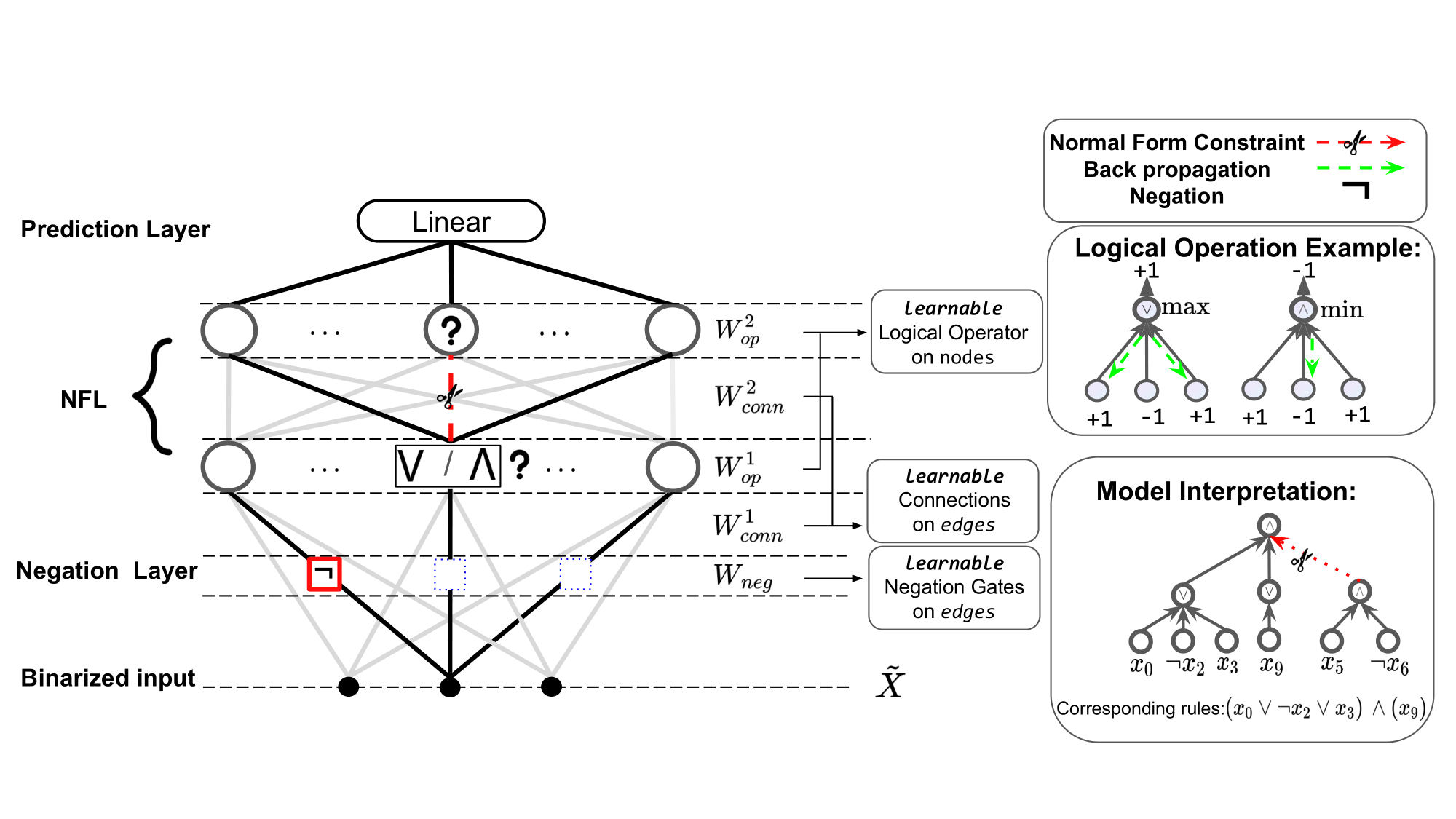
Figure 1: Overall Structure.

To achieve the goal in Section 3.3, we propose a neural network that can be optimized end to end. Specifically, we identify four key challenges: (1) How can neurons be designed to dynamically select suitable logical operations to flexibly represent CNF and DNF? (2) How to support the negation operation? (3) How to efficiently learn logical connections when there is a big search space? and (4) How to effectively optimize the rule-based neural network and tackle the gradient vanishing problem?

Model Structure. To tackle the first challenge, we design the Normal Form Layer (NFL) such that neurons can adaptively select AND or OR logical operations, and the connections between neurons can represent CNF and DNF rules. Then, we invent a negation layer that integrates negation gates to effectively attack the challenge of negation operation for input binary features. To tackle the third challenge, we further devise a Normal Form Constraint (NFC) for efficiently learning connections between neurons. Last, to circumvent gradient vanishing, we adopt +/-1 for neuron values coupled with logical activation by max/min functions. And we apply adaptive gradient update with a Straight-Through Estimator to effectively optimize the proposed model. The framework of NFRL is depicted in Figure 1.

Given an input sample, the original feature vector $\mathbf{x}$ is transformed to its binarized version $\mathbf{\tilde{x}}$. Then, $\mathbf{\tilde{x}}$ will be connected to the first NFL to achieve the first level of logical operations (conjunction or disjunction). During this process, we also integrate a negation layer, which assigns a negation gate to each of the connections to determine if the logical operation takes the original binary feature or its negation as the literal. After this, another NFL follows to achieve the second level of logical operation. Up to now, we gain the rules $\mathfrak{R}$ needed for prediction, and each neuron in the second NFL represents a rule in $\mathfrak{R}$. Last, we adopt a linear layer to weighted aggregate the rules for calculating logits for all classes.

Binary Neuron Values. A key characteristic of NFRL is that the values of all neurons (except for the predicted logits) are constrained to be +1 or -1. The binarized feature input is also constrained to +/-1 as introduced in Section 3.2. Importantly, the reason for constraining values to +/-1 instead of 0/1 as existing works Wang et al. (2020, 2021), is that this design significantly enhances the optimization process by avoiding the gradient vanishing problem. The details regarding optimization and analyses of gradient vanishing will be discussed in Section 4.4.

4.2 Normal Form Layer (NFL)

Neuron Operator Selection. Motivated by the nested structure of CNF and DNF, we propose to stack two Normal Form Layers (NFLs) to effectively express CNF and DNF rules. Each NFL contains K logical neurons $\{u_{1},u_{2},\ldots,u_{K}\}$ where each neuron represents a logical operator selected from either AND ($\wedge$) or OR ($\vee$). We use $\mathbf{w}_{op}\in\mathbb{R}^{K}$ to parameterize the logical operator selection process of all K neurons. Given the weight $\mathbf{w}_{op}^{i}$ for a neuron $u_{i}$, we further get the binary version by taking the sign of it: $\tilde{\mathbf{w}}_{op}^{i}=sign(\mathbf{w}_{op}^{i})\in\{+1,-1\}$. Then, the operator selection mechanism is defined as:

$$u_{i}=\begin{cases}\land,\&\text{if}\ \tilde{w}_{op}^{i}=1\\ \lor,\&\text{otherwise}\end{cases}$$ (1)

Neuron Connection. Similar to multi-layer perceptron, we learn a weight matrix $\mathbf{W}_{conn}$ recording weights for pairs of neurons from two consecutive layers, e.g., $\mathbf{W}_{conn}^{i,j}\in\mathbb{R}$ is the weight for neurons $u_{i}$ and $u_{j}$ from two consecutive layers. In NFRL, we only need to learn two weight matrices, one for (input layer, 1st NFL), the other for (1st NFL, 2nd NFL). Given the learned $\mathbf{W}_{conn}$, we further turn it into a binary version by taking the sign: $\widetilde{\mathbf{W}}_{conn}^{i,j}=sign(\mathbf{W}_{conn}^{i,j})\in\{+1,-1\}$, representing the connection between the involving two layers – neurons $u_{i}$ and $u_{j}$ are connected if $\widetilde{\mathbf{W}}_{conn}^{i,j}=1$, neurons are not connected otherwise. Given this, we define the output $v_{i}$ of a neuron $u_{i}$ in NFL as:

$$v_{i}=\begin{cases}\underset{\widetilde{\mathbf{W}}_{conn}^{i,j}=1}{\bigwedge}v_{j},&\text{if}\,\,u_{i}=\land\\ \underset{\widetilde{\mathbf{W}}_{conn}^{i,j}=1}{\bigvee}v_{j},&\text{if}\,\,u_{i}=\lor\end{cases}$$ (2)

where $v_{j}$ are neurons from the previous layer that are connected to $u_{i}$, i.e., $\widetilde{\mathbf{W}}_{conn}^{i,j}=1$.

Logical Activation Functions. In propositional logic, for a scenario involving m inputs: for the AND operation, the output will be +1 if and only if all the connected neurons are +1; for the OR operation, the output will be +1 as long as at least one connected neuron is +1. Based on these principles, we propose to adopt max and min functions to implement the logical operations as logical activation functions in NFRL. The AND ($\land$) operation can be defined as the minimum of its connected inputs, and the OR operation is defined as the maximum of its connected inputs:

$$v_{i}=\begin{cases}\underset{\widetilde{\mathbf{W}}_{conn}^{i,j}=1}{\text{min}}v_{j},&\text{if}\,\,u_{i}=\land\\ \underset{\widetilde{\mathbf{W}}_{conn}^{i,j}=1}{\text{max}}v_{j},&\text{if}\,\,u_{i}=\lor\end{cases}$$ (3)

Compared to accumulative-multiplication-based activation functions proposed in prior works Wang et al. (2020, 2021), this min-max-based method is more friendly for backpropagation and preventing the gradient vanishing problem, which will be detailed in Section 4.4.

4.3 Negation Layer

Most existing works Wang et al. (2020, 2021) only support {AND, OR}, which is not functional complete Mendelson (1997); Enderton (2001) for propositional logic. We aim to enable NFRL to theoretically express any form of rule by supporting a functionally complete set of logical operators {AND, OR, NEGATION}. To achieve this, we introduce the negation layer to achieve the negation operation on features.

Because the negation is exerted on input features, we apply the negation layer after the input layer. Specifically, for each connection between a neuron $v_{j}$ from the input layer $\tilde{\mathbf{x}}$ and a neuron $u_{i}$ from the 1st NFL, we further design a negation gate to determine if we input the original input $v_{j}$ or the negation $\neg v_{j}$ to $u_{i}$. For such a gate, we learn a weight $\mathbf{W}_{neg}^{i,j}\in\mathbb{R}$ and take the sign of the learned weight to get the binary version: $\widetilde{\mathbf{W}}_{neg}^{i,j}=sign(\mathbf{W}_{neg}^{i,j})\in\{+1,-1\}$, with which we define the negation operation as: $Neg(v_{j},\widetilde{\mathbf{W}}_{neg}^{i,j})=v_{j}\times\widetilde{\mathbf{W}}_{neg}^{i,j}$.

4.4 Optimization

Learning such a binary neural network is challenging. The core challenge lies in calculating gradients for the discrete functions in the model – the $sign(\cdot)$, $max(\cdot)$ and $min(\cdot)$ – all of which are non-differentiable.

Gradient of the Sign Function. Motivated by the idea of searching discrete solutions in continuous space Courbariaux et al. (2015). We adopt the Straight-Through Estimator (STE) algorithm that allows for the propagation of gradients through a non-differentiable operation during backpropagation. In practice, the STE assumes the derivative of the sign function w.r.t. its input is 1, effectively allowing the gradient to “pass through" the non-differentiable operation unchanged:

$$\frac{\partial sign(x)}{\partial x}=1.$$ (4)

Gradient of Logical Activation Functions. The max and min operations, when applied to input neurons, identify the maximum or minimum value across inputs. Previous work Lowe et al. (2022) primarily applies these activation functions in continuous scenarios with paired inputs. We extend this approach to handle discrete and multiple inputs. In pairwise situations, a logical operator selects one or two inputs, making it straightforward to assign a gradient of 1 to the selected input and update the parameters equally. However, extending this to multiple inputs allows several neurons to be satisfied simultaneously for some rules, while others involve a relatively small number of satisfied neurons. This discrepancy within the rule sets makes it inappropriate to expect equalized gradient updates across all neurons. Complex rules should be updated smoothly due to the large number of involved features, while specific rules require more rapid updates. During the backward pass of gradient computation, if multiple neurons share the same maximum or minimum value, the gradient will be evenly distributed among all selected neurons. Formally, given an input vector $\mathbf{x}$ with elements $\{x_{1},x_{2},\ldots\}$, the gradient of an input element $x_{i}$ is:

$$\centering\frac{\partial\max(\mathbf{x})}{\partial x_{i}} =\frac{1}{\sum_{j}\mathbb{I}(x_{j}=\max(\mathbf{x}))},$$ (5)

$$\frac{\partial\min(\mathbf{x})}{\partial x_{i}} =\frac{1}{\sum_{j}\mathbb{I}(x_{j}=\min(\mathbf{x}))}.$$

Gradient Vanishing. Our innovative design circumvents the gradient vanishing problem that plagues existing methods Wang et al. (2020, 2021). There are two primary causes of the gradient vanishing in these prior works. First, they design the binary states of their models with values 0 and 1, leading to numerous neurons producing an output of 0. These 0 values in the forward pass can nullify the gradients in the backward pass. Second, these prior methods rely on accumulative multiplications to implement AND and OR for logical activation functions. For example, the AND operation can be implemented as $AND(\mathbf{x})=\prod_{i}x_{i}$ when $x_{i}\in\{0,1\}$. This results in the situation where the gradient of an input depends on the product of others: $\partial AND(\mathbf{x})/\partial x_{j}=\prod_{i\neq j}x_{i}$. As the input dimension increases, this gradient as a product is likely to approach 0. A detailed discussion is included in Appendix F.

In contrast, we adopt +/-1 for defining the binary states in the neural network to prevent generating 0 outputs and 0 gradients. Furthermore, our simple yet powerful logical activation functions do not rely on a product. The straightforward gradient calculation introduced in Equation 5 alleviate the gradient vanishing problem.

4.5 Normal Form Constraint (NFC)

Next, we turn our attention to one critical challenge of NFRL – learning the connections between the two NFLs is computationally intensive. Assuming we have K neurons in each NFL, we need to learn and determine $K^{2}$ potential connections, significantly weakening the efficiency and efficacy of the model. Hence, we design a normal form constraint to keep the learned rules in CNF and DNF, and at the same time, reduce the search space for learning the connections between two NFLs. Specifically, since CNF and DNF are in a nested structure, where the operations in the two levels have to be different (CNF is the conjunction of disjunction rules, DNF is the opposite), we have the constraint that only different types of neurons from the two NFLs can be connected. For neurons $u_{i}$ and $u_{j}$ from two NFLs, we define a mask parameter $M^{i,j}$ as:

$$M^{i,j}=\tilde{\mathbf{w}}^{i}_{op}\oplus\tilde{\mathbf{w}}^{j}_{op}=-\tilde{\mathbf{w}}^{i}_{op}\tilde{\mathbf{w}}^{j}_{op},$$ (6)

where $\oplus$ denoted the XOR operation. Then, there is a connection between $u_{i}$ and $u_{j}$ if $M^{i,j}\times\widetilde{\mathbf{W}_{conn}^{i,j}}=1$, otherwise no connection. And during optimization, we only update $\mathbf{W}_{conn}^{i,j}$ when $M^{i,j}=1$.

Assuming there are $C_{1}$ and $C_{2}$ conjunction neurons in two NFLs respectively, and $D_{1}$ and $D_{2}$ disjunction neurons respectively ($C_{1}+D_{1}=C_{2}+D_{2}=K$), then potential connections under NFC is $C_{1}D_{2}+C_{2}D_{1}\leq K^{2}$. The empirical study in Section 5.5 demonstrates that NFC benefits both the efficiency and efficacy of the model while guaranteeing the learned rules are in CNF and DNF.

Dataset	Ours	RRL	CRS	C4.5	CART	SBRL	CORELS	LR	SVM	PLNN(MLP)	RF	LightGBM	XGBoost
adult	81.24	80.72	80.95	77.77	77.06	79.88	70.56	78.43	63.63	73.55	79.22	80.36	80.64
bank	77.18	76.32	73.34	71.24	71.38	72.67	66.86	69.81	66.78	72.40	72.67	75.28	74.71
chess	79.20	78.83	80.21	79.90	79.15	26.44	24.86	33.06	79.58	77.85	75.00	80.58	80.66
connect-4	72.15	71.23	65.88	61.66	61.24	48.54	51.72	49.87	69.85	64.55	62.72	70.53	70.65
letRecog	95.82	96.15	84.96	88.20	87.62	64.32	61.13	72.05	95.57	92.34	96.59	96.51	96.38
magic04	86.58	86.33	80.87	82.44	81.20	82.52	77.37	75.72	79.43	83.07	86.48	86.67	86.69
wine	98.80	98.23	97.78	95.48	94.39	95.84	97.43	95.16	96.05	76.07	98.31	98.44	97.78
activity	98.80	98.17	5.05	94.24	93.35	11.34	51.61	98.47	98.67	98.27	97.80	99.41	99.38
dota2	59.96	60.12	56.31	52.08	51.91	34.83	46.21	59.34	57.76	59.46	57.39	58.81	58.53
facebook	90.93	90.27	11.38	80.71	81.50	31.16	34.93	88.62	87.20	89.43	87.49	85.87	88.90
fashion	87.68	89.01	66.92	80.49	79.61	47.38	38.06	84.53	84.46	89.36	88.35	89.91	89.82
AvgRank	2.72	3.81	7.91	8.73	9.64	10.36	11.55	8.91	7.91	6.91	6.00	3.18	3.18

Table 1: F1 scores (%) across 11 datasets. The first seven baselines are interpretable, and the last four are non-interpretable. Best performances are in bold.

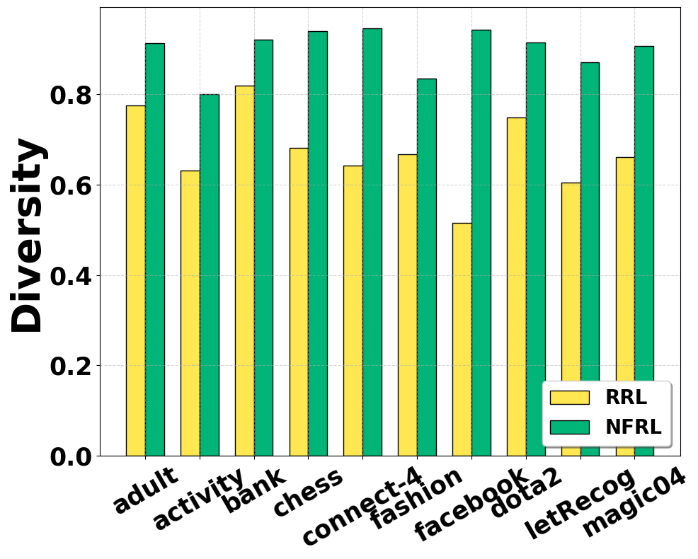
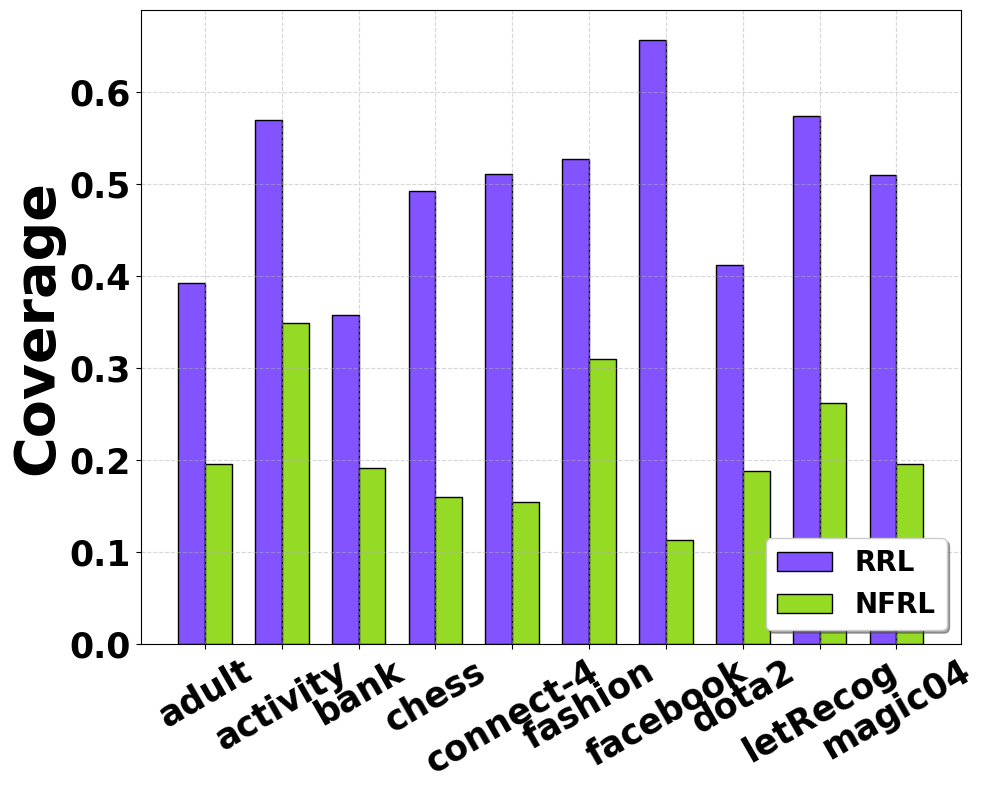
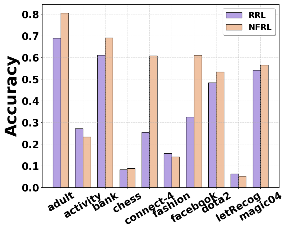
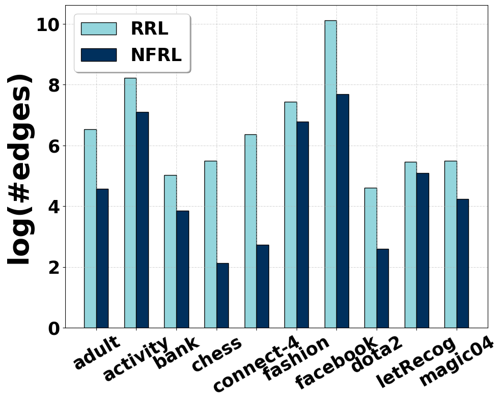
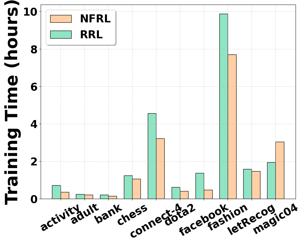
Figure 2: Comparison of Various Metrics. (a) Diversity. (b) Coverage. (c) Accuracy. (d) Average Rule Length. (e) Comparison of Computational Time.

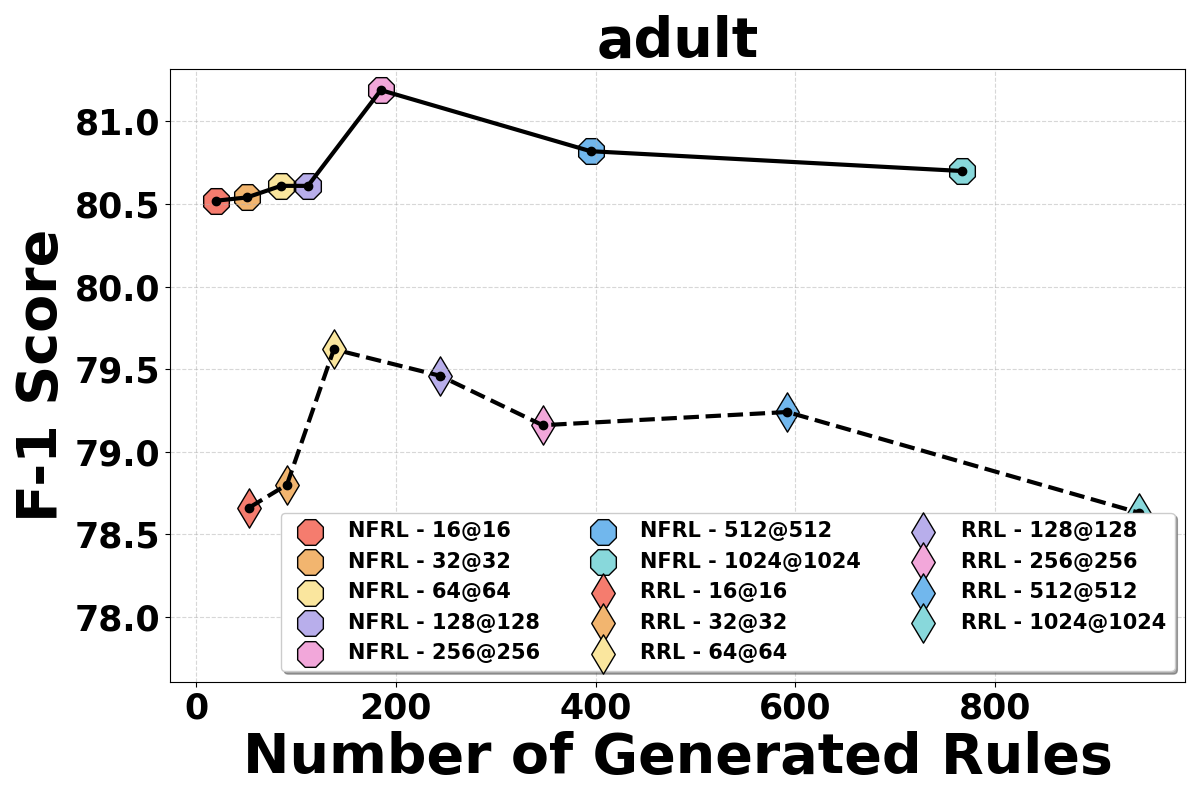
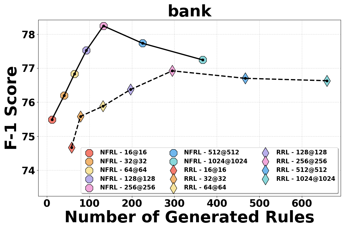
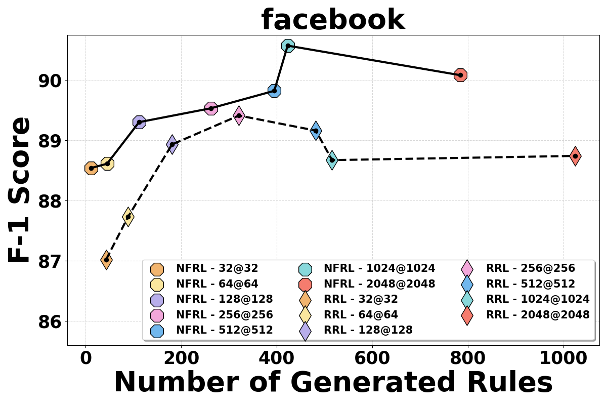
Figure 3: Comparison of F1 Scores for NFRL and RRL with Different Numbers of Generated Rules.

5 Experiment

In this section, we conduct comprehensive experiments to evaluate the proposed model and answer the following research questions: RQ1: How does NFRL perform w.r.t. classification accuracy compared to SOTA baselines? RQ2: What is the quality of the rules learned by NFRL? RQ3: How efficient NFRL is in terms of model complexity and training time? RQ4: What are the effects of the proposed Negation Layer, NFC, and the impact of different binning functions on NFRL? RQ5: What are the impacts of different hyperparameters in NFRL?

5.1 Experimental Settings

Datasets. We conduct extensive experiments on seven small datasets (adult Becker and Kohavi (1996), bank-marketing Moro et al. (2012), chess Bain and Hoff (1994), connect-4 Tromp (1995), letRecog Slate (1991), magic04 Bock (2007), wine Aeberhard and Forina (1991)) and four large datasets (activity Reyes-Ortiz et al. (2012), dota2 Tridgell (2016), facebook mis (2020), fashion-mnist Xiao et al. (2017)). These datasets are commonly utilized for evaluating classification performance and assessing model interpretability Letham et al. (2015); Wang et al. (2017); Yang et al. (2017). Details of these datasets are shown in Appendix A. Datasets are classified as ‘Discrete’ or ‘Continuous’ depending on whether their features are exclusively of one type. A dataset incorporating both types is categorized as ’Mixed’. We employ 5-fold cross-validation for evaluation. We report the average performance over five iterations in this paper.

Performance Evaluation. We use the F1 score (Macro-average for multi-class cases) for assessing classification performance. Additionally, for each dataset, we rank NFRL and baselines based on their performance from 1 (the best performance) to 13 (the worst). We compare models across all datasets using their average rank Demšar (2006) as a comprehensive evaluation (the lower the better).

Reproducibility. In NFRL, there are two NFLs. The number of logical neurons within these layers is grid-searched from 32 to 4096, depending on the dataset’s complexity. For training, we employ cross-entropy loss and use L2 regularization to limit model complexity. The regularization term’s coefficient in the loss function is searched from $10^{-5}$ to $10^{-9}$. The number of bins in the feature binarization layer is selected from $\{15,30,50\}$. We train the model using the Adam optimizer Kingma and Ba (2014) with a batch size of 32. For small datasets, the model is trained for 400 epochs, with the learning rate decreasing by 10% every 100 epochs. For large datasets, it is trained by 100 epochs, with a similar learning rate reduction every 20 epochs. The settings for baselines follow  Wang et al. (2021). We implement NFRL with PyTorch  Paszke et al. (2019). For the baseline comparison, we reuse the high-quality code base released by  Wang et al. (2021). Experiments are conducted on a Linux server with an NVIDIA A100 80GB GPU. All code and data are available at https://anonymous.4open.science/r/NFRL-27B4/.

Baselines. In our comparative analysis, we assess the performance of NFRL against a diverse array of methods, categorized into two main groups: interpretable and more complex but non-interpretable models. The interpretable models include a variety of rule-based approaches such as RRL Wang et al. (2021), Concept Rule Sets (CRS) Wang et al. (2020), C4.5 Quinlan (2014), CART Breiman (2017), Scalable Bayesian Rule Lists (SBRL) Yang et al. (2017), and Certifiably Optimal Rule Lists (CORELS) Angelino et al. (2018), in addition to the linear model Logistic Regression (LR) Kleinbaum et al. (2008). These models are selected for their notable transparency and ease of interpretability. Conversely, the complex models include Piecewise Linear Neural Network (PLNN) Chu et al. (2018), Support Vector Machines (SVM) Schölkopf and Smola (2002), Random Forest (RF) Breiman (2001), LightGBM Ke et al. (2017), and XGBoost Chen and Guestrin (2016). PLNN operates as a variant of the Multi-layer Perceptron (MLP) with piecewise linear activation functions, such as ReLU Nair and Hinton (2010), while RF, LightGBM, and XGBoost are sophisticated ensemble models that aggregate decisions from multiple decision trees to bolster performance. Within this landscape, RRL emerges as the premier interpretable baseline, illustrating the efficacy of rule-based models in terms of transparency. Meanwhile, LightGBM and XGBoost distinguish themselves as the leading complex models, achieving the highest performance metrics albeit at the expense of interpretability.

5.2 Classification Performance (RQ1)

We evaluate the F1 score of NFRL against a set of competitive baselines, including interpretable models and non-interpretable ones. The results are shown in Table 1, where the first seven datasets are small datasets and the last four are large datasets. Baseline results are taken from  Wang et al. (2021) to ensure a fair comparison due to the consistent experimental setup. NFRL achieves the best F1 score on four datasets – bank-marketing, connect-4, wine, and facebook, suggesting a robust classification capability in a variety of contexts.

The average ranking places NFRL among the best, even better than SOTA uninterpretable ensemble models LightGBM and XGBoost (2.72 vs. 3.18). This shows the exceptional performance of NFRL over a range of datasets. It excels beyond traditional interpretable models like CART and C4.5, rule-based models like RRL (the SOTA rule-based interpretable method) and CRS, as well as more advanced but not interpretable models such as RF, SVM, and MLP. NFRL performs effectively on both small and large datasets, and datasets with different types of features, demonstrating its strong scalability and generalizability. Thus, NFRL is a potent method for tasks that demand interpretability alongside accuracy.

5.3 Rule Quality (RQ2)

Next, we aim to evaluate the quality of learned rules from different rule-learning models. We benchmark NFRL against RRL, the SOTA rule-based neural network, to establish a comparative baseline. We first compare rules from these two models by various existing rule quality metrics, and then conduct a simulation experiment to verify if models can recover underlying rules in data.

Ground-Truth Rules	Rules_Ours	Rules_RRL
$(x_{1}\lor x_{2})\land\lnot x_{3}$	$x_{1}\land\lnot x_{3}$	$x_{1}\land x_{2}\land x_{3}$
	$x_{2}\land\lnot x_{3}$	$x_{1}$
	$x_{1}\land x_{2}\land\lnot x_{3}$	$x_{2}$
		$x_{2}\land x_{3}$
$x_{1}\lor(\lnot x_{2}\land\lnot x_{3})$	$\lnot x_{2}\land\lnot x_{3}$	$x_{1}$
	$x_{1}$	$x_{2}$
		$x_{3}\lor x_{2}\lor(x_{2}\lor x_{1})$
$x_{1}\land\lnot x_{2}\land x_{3}$	$x_{1}\land\lnot x_{2}\land x_{3}$	$x_{1}\land x_{3}$
		$x_{2}\lor x_{2}$
		$(x_{1}\land x_{3})\land x_{1}$
$x_{1}\lor\lnot x_{2}\lor\lnot x_{3}$	$x_{1}\lor\lnot x_{2}\lor\lnot x_{3}$	$x_{2}\land x_{3}$
		$(x_{2}\land x_{3})\land x_{2}\land x_{3}$

Table 2: Logical rules obtained from NFRL trained on the synthetic dataset.

Rules	Support_no	Support_yes	Coverage
$(\text{duration}>146.719\land\lnot\text{job}\in\{\text{housemaid},\text{entrepreneur}\}\land$	$-0.4159$	$0.3929$	$0.4236$
$\lnot\text{month}\in\{\text{nov},\text{mar},\text{feb}\}\land\text{balance}<1757.276)$
$\bigvee(\lnot\text{duration}<850.975\land\lnot\text{job}=\text{technician}\land\text{month}=\text{mar})$
$\bigvee(\text{duration}>146.719\land\lnot\text{month}=\text{jan}\land\lnot\text{contact}=\text{unknown})$
$\bigvee(\text{duration}>19.057\land\lnot\text{age}>67.878\land\text{month}=\text{oct}\land\lnot\text{day}<5.569)$
$\bigvee(\lnot\text{duration}<850.975\land\text{age}<66.978\land$
$\lnot\text{job}=\text{housemaid}\land\lnot\text{month}=\text{jan}\land\lnot\text{poutcome}=\text{success})$
$\bigvee(\text{duration}>59.781\land\lnot\text{job}=\text{unknown})$
$\bigvee(\text{duration}>19.057\land\lnot\text{age}>28.949)$
$\bigvee(\text{duration}>59.781\land\lnot\text{age}>67.878\land\lnot\text{job}\in\{\text{self-employed},\text{housemaid}\}\land$
$\lnot\text{month}\in\{\text{oct},\text{nov}\}\land\lnot\text{loan}=\text{yes}\land\lnot\text{default}=\text{yes})$
$(\text{duration}>59.781\land\lnot\text{month}\in{\{\text{jul},\text{aug}\}}\land\text{balance}<1537.899\land$	$0.3314$	$-0.3539$	$0.3617$
$\text{previous}>1.028\land\text{pdays}<229.326)$
$\bigvee(\lnot\text{month}=mar\land\lnot\text{poutcome}=\text{success}\land$
$102.083<\text{pdays}<304.124\land\text{previous}<6.754)$
$(\lnot\text{month}=\text{aug}\land\lnot\text{age}<12.397\land\text{campaign}>0.066\land\text{day}<33.738\land$	$-0.5581$	$0.5437$	$0.3319$
$\text{pdays}<244.292)$

Table 3: Logical rules obtained from NFRL trained on the bank-marketing data set.

5.3.1 Rule Quality Metrics

Following prior work Yu et al. (2023); Lakkaraju et al. (2016), we adopt evaluation metrics including diversity, coverage, and single rule accuracy. We conduct extensive experiments across 10 datasets, as shown in Figure 2 and detailed in Appendix C, . Accuracy measures the prediction accuracy using a single rule for the instances it covers; higher accuracy of a single rule indicates better meaningfulness, as it can make more correct predictions when applied alone. Coverage evaluates the proportion of data instances a rule covers; lower coverage means the rule is easier for human experts to distinguish, as it covers a smaller set of instances. Diversity quantifies the overlap ratio between pairs of rules; higher diversity indicates better generalization power, as each rule covers instances in different scenarios with only a small overlap with other rules. NFRL consistently produces rules with superior results: higher accuracy, greater diversity, and lower coverage deviation, indicating that rules learned by the proposed method are easier to distinguish and exhibit better prediction and generalization power.

5.3.2 Simulation Experiment

We evaluate NFRL’s capability to accurately learn underlying rules that generate the data, serving as an assessment of the model’s proficiency in learning accurate rules.

Setup. Our goal is to generate synthesis data based on predefined logical rules, and then train the rule-based models to evaluate whether the models can reconstruct the ground-truth rules. To generate a dataset based on a rule, we initiate the simulation by defining three probability parameters, $\mathbf{p}=(p_{1},p_{2},p_{3})$ corresponding to three feature variables $\{x_{1},x_{2},x_{3}\}$, each independently drawn from a uniform distribution $U(0,1)$ for $i=1,2,3$. Utilizing them as three Bernoulli parameters, we generate $X_{gen}\in\mathbb{R}^{3\times 50000}$ by repeating Bernoulli sampling, a dataset comprising $n=50000$ binary vectors (samples), with each vector of length 3 corresponding to the elements of $\mathbf{p}$. These vectors are created through sampling from a Bernoulli distribution $Bernoulli(p_{i})$ for each $p_{i}$, yielding binary outcomes. Subsequently, labels are assigned to the binary vectors based on specific logical rules. For instance, if we define a rule $x_{1}\land x_{2}\land x_{3}\rightarrow 1$, a vector (sample) is labeled as 1 if all three features are 1. We design four different types of rules, as shown as ‘Ground-Truth Rules’ in Table 2. We split data into a training set and a test set as 50% vs. 50%. Both NFRL and RRL are set to have a dimension of $64@64$ for their logical layers.

Results. We demonstrate that NFRL is not only capable of providing accurate predictions but also can learn the ground-truth rules underlying the data. The results are presented in Table 2. Given the simple structure of the rules that generate the data, both NFRL and RRL achieve a near 100% accuracy rate. However, NFRL excels by not just delivering precise predictions but also by comprehensively capturing the structure of the ground-truth rules. In contrast, RRL, which lacks support for flexible architecture, often learns rules that are overly simplistic and repetitive even with the doubled size of input features. For instance, consider the Ground-Truth Rule $x_{1}\land\lnot x_{2}\land x_{3}$. NFRL is capable of learning this exact structural rule, whereas RRL is unable to do so. It emphasizes the superior ability of NFRL to learn complex logical rules. Additionally, we report the results of RRL with a naive negation setting in Appendix C for a fair comparison. NFRL still performs better than the baseline.

5.4 Efficiency (RQ3)

We evaluate the learning efficiency by the number of learned rules, the length of the learned rules, and computational time. Generally, very large rule sets with many conditions per rule are challenging to understand. Thus, fewer rules with shorter lengths are desired. We explore the relationship between the number of learned rules and F1 score in Figure 3 and Appendix D, finding that NFRL consistently achieves higher performance with fewer rules compared to RRL. Additionally, we evaluate the average length of the learned rules in NFRL across different datasets in Figure 2 and Appendix D. We observe that NFRL consistently produces shorter rules, with an average length of fewer than eight, making the rules easier for humans to understand. The computational time of the proposed method is shown in Figure 2. We observe that NFRL consistently converges faster than the best baseline across all datasets. Overall, the proposed method consistently produces more concise rules of reasonable size in less computational time, facilitating easier comprehension of the results.

5.5 Ablation Study (RQ4)

Negative Layer and NFC. To demonstrate the effectiveness of the Negation Layer and Normal Form Constraint (NFC), we compare NFRL trained with and without these components. The Negation Layer supports negation operations in learned rules for functional completeness, while NFC narrows the search space for learning connections between logical layers, both aiming to enhance model performance. Table 6 in Appendix E shows F1 scores for NFRL and its variants on a small dataset (bank) and a large dataset (activity). The decreases in F1 scores when the Negation Layer and NFC are removed underscore their importance. Another reason for incorporating NFC is to enhance learning efficiency. With all other factors constant, we compare the training time for NFRL with and without NFC. As shown in Table 7 in Appendix E, NFC reduces training time by 11.22% and 25% for the activity and bank datasets, respectively, underscoring its necessity and importance.

Binning Function. Next, we study how NFRL performs with different binning functions. We consider four binning methods: RanInt Wang et al. (2021), the default in this paper introduced in Section 3.2; KInt Dougherty et al. (1995), which uses K-means clustering to divide the feature value range; EntInt Wang et al. (2020), which partitions the feature range to reduce class label uncertainty (entropy) within each bin; and AutoInt Zhang et al. (2023), a learning-based method that optimizes bins during model training.

The F1 scores of NFRL with different binning functions are shown in Table 8 in Appendix E. NFRL demonstrates strong flexibility with various binning methods, with RanInt achieving the best performance. The randomness in interval selection introduces stochastic diversity in the binning process, helping to prevent overfitting. Additionally, its computational efficiency and intuitive design may be advantageous for this problem. In contrast, the KInt method clusters features based solely on feature values, neglecting the target variable, which can result in bins that do not effectively represent the relationship with the intended output. EntInt incorporates label data to form bins that minimize entropy, potentially enhancing predictive accuracy. Finally, while the learning-based AutoInt method offers adaptability, its computationally intensive parameter search can pose optimization challenges in practice.

5.6 Hyperparameter Study (RQ5)

NFL Dimension K. We analyze the effect of layer dimension K (number of neurons) in the two NFLs. Larger K increases model complexity, improving performance but risking overfitting. We test dimensions K in $\{32@32,64@64,128@128,256@256,512@512,$ $1024@1024,2048@2048\}$ on a small dataset (bank) and a large dataset (activity) shown in Figure 4 in Appendix B. The F1 score rises initially and then falls as K increases, peaking at $1024@1024$ for activity data and $128@128$ for bank data. Thus, the activity dataset benefits from larger models, while the bank dataset performs best with smaller models, indicating that optimal model size depends on dataset complexity.

L2 regularization $\lambda$. We then examine the impact of the L2 regularization weight $\lambda$, which controls NFRL complexity. A larger $\lambda$ reduces model complexity, resulting in fewer and simpler logical rules. We vary $\lambda$ from $1e^{-5}$ to $1e^{-9}$ and show the model’s performance in Figure 5 in Appendix B. The F1 score initially rises and then falls as $\lambda$ increases. This indicates that performance improves when $\lambda$ is appropriately chosen. To avoid overfitting or underfitting, a balanced $\lambda$ is essential for optimal model complexity.

5.7 Model Interpretation

Table 3 presents a set of three most discriminative rules extracted from NFRL, which has been trained on the bank-marketing dataset to identify customer profiles likely to subscribe to a term deposit through telesales. These rules offer a detailed profile of potential subscribers by highlighting specific conditions that, when met, increase the likelihood of subscription. ‘Support_yes’ denotes the contribution of the rule to the positive label – a large positive value indicates that if the rule is true for an input customer, the probability of a subscription is high. On the other hand, ‘Support_no’ denotes the contribution of the rule to the negative label – a high positive value suggests a high likelihood against subscription given the rule is true. ‘Coverage’ represents the ratio of samples in the training data that satisfies this rule, showing the prevalence of the rules.

Thanks to the transparency, we can conclude from the insightful interpretations that subscriptions are less probable in colder seasons, possibly due to a general reluctance to engage in financial decisions during holiday periods. Our model highlights a correlation between effective marketing and longer call duration, implying that interest in deposits often results in extended dialogues. Additionally, our model indicates that housemaids, entrepreneurs, and self-employed individuals are less inclined towards term deposits, potentially due to entrepreneurs’ need for flexibility to support their business ventures, the inherent financial instability faced by self-employed individuals, and the limited disposable income of housemaids. Analysis further reveals age-related trends in communication length, with younger individuals tending towards shorter calls and middle-aged clients engaging in longer discussions. This underscores our model’s utility in reflecting plausible real-world behaviors rather than asserting direct explanations of them.

6 Conclusion

In this work, we introduced the Normal Form Rule Learner (NFRL), an innovative framework that employs a discrete neural network for learning logical rules in both Conjunctive and Disjunctive Normal Forms (CNF and DNF), aiming to enhance interpretability and classification accuracy. Instead of adopting a deep, complex structure, NFRL incorporates two Normal Form Layers (NFLs) equipped with flexible AND and OR neurons, a Negation Layer for implementing negation operations, and a Normal Form Constraint (NFC) to optimize neuron connections. This architecture can be optimized using the Straight-Through Estimator in an end-to-end backpropagation fashion. Extensive experiments demonstrate NFRL’s superiority in terms of prediction accuracy and interpretability compared to both traditional rule-based models and advanced, non-interpretable methods. In the future, we plan to study how to extend this model for other applications, such as recommendation or text processing.

Appendix A Dataset Statistics

In Table  4, the first nine data sets are small, while the last four are large. The "Discrete" or "Continuous" feature type indicates that all features in the data set are either discrete or continuous, respectively. The "Mixed" feature type indicates that the corresponding data set contains both discrete and continuous features.

Dataset	#instances	#classes	#features	feature type
adult	32561	2	14	mixed
bank	45211	2	16	mixed
chess	28056	18	6	discrete
connect-4	67557	3	42	discrete
letRecog	20000	26	16	continuous
magic04	19020	2	10	continuous
wine	178	3	13	continuous
activity	10299	6	561	continuous
dota2	102944	2	116	discrete
facebook	22470	4	4714	discrete
fashion	70000	10	784	continuous

Table 4: Datasets statistics

Appendix B Hyperparameter Study

NFL Dimension K. We analyze the effect of layer dimension K (number of neurons) in the two NFLs. A larger K increases model complexity, potentially improving performance but risking overfitting. We test dimensions K in $\{32@32,64@64,128@128,256@256,$ $512@512,1024@1024,2048@2048\}$ on a small dataset (bank) and a large dataset (activity) shown in Figure 4. The F1 score initially rises and then falls as K increases, peaking at $1024@1024$ for the activity dataset and $128@128$ for the bank dataset. This indicates that the activity dataset benefits from larger models, while the bank dataset performs best with smaller models, suggesting optimal model size depends on dataset complexity.

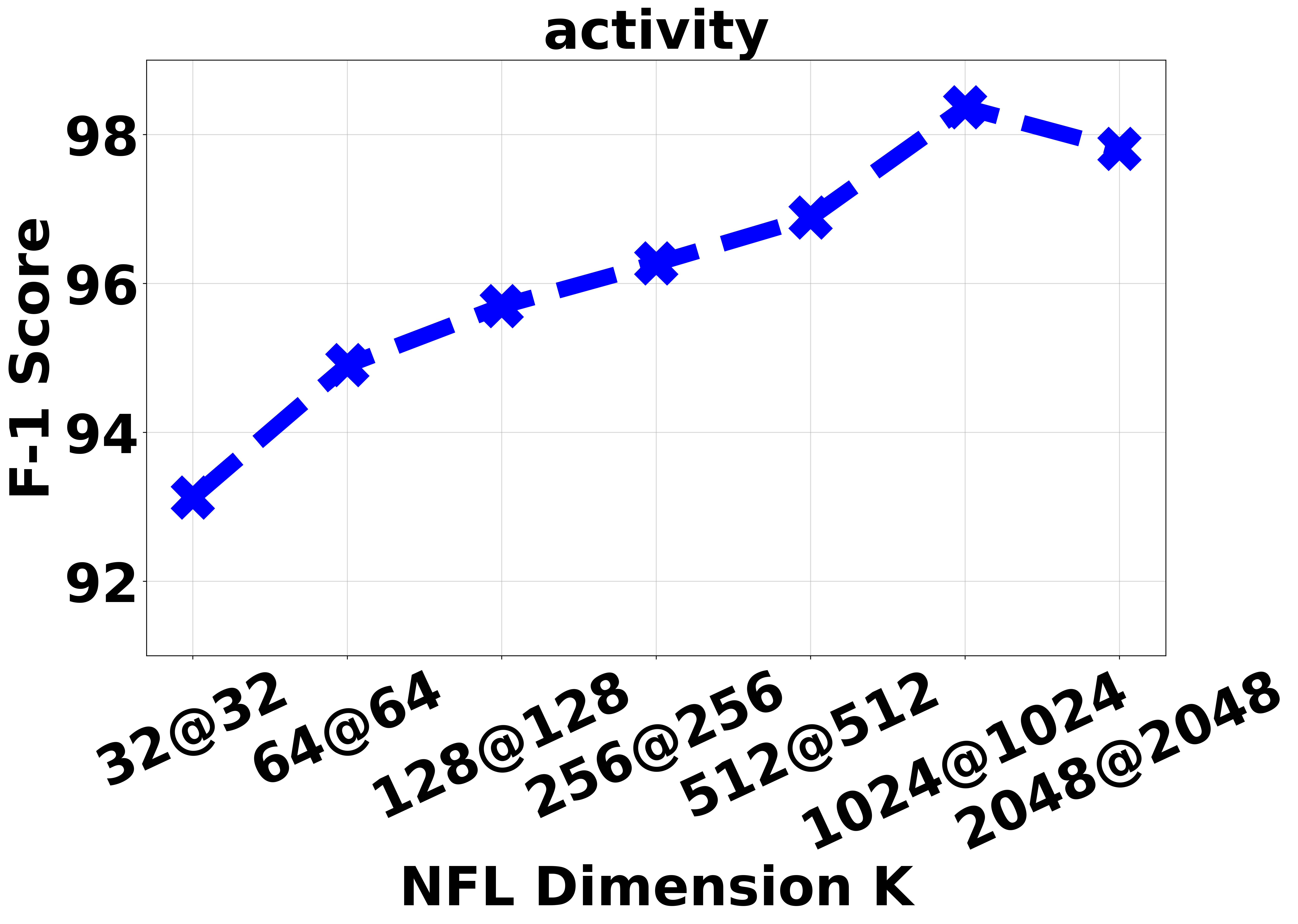
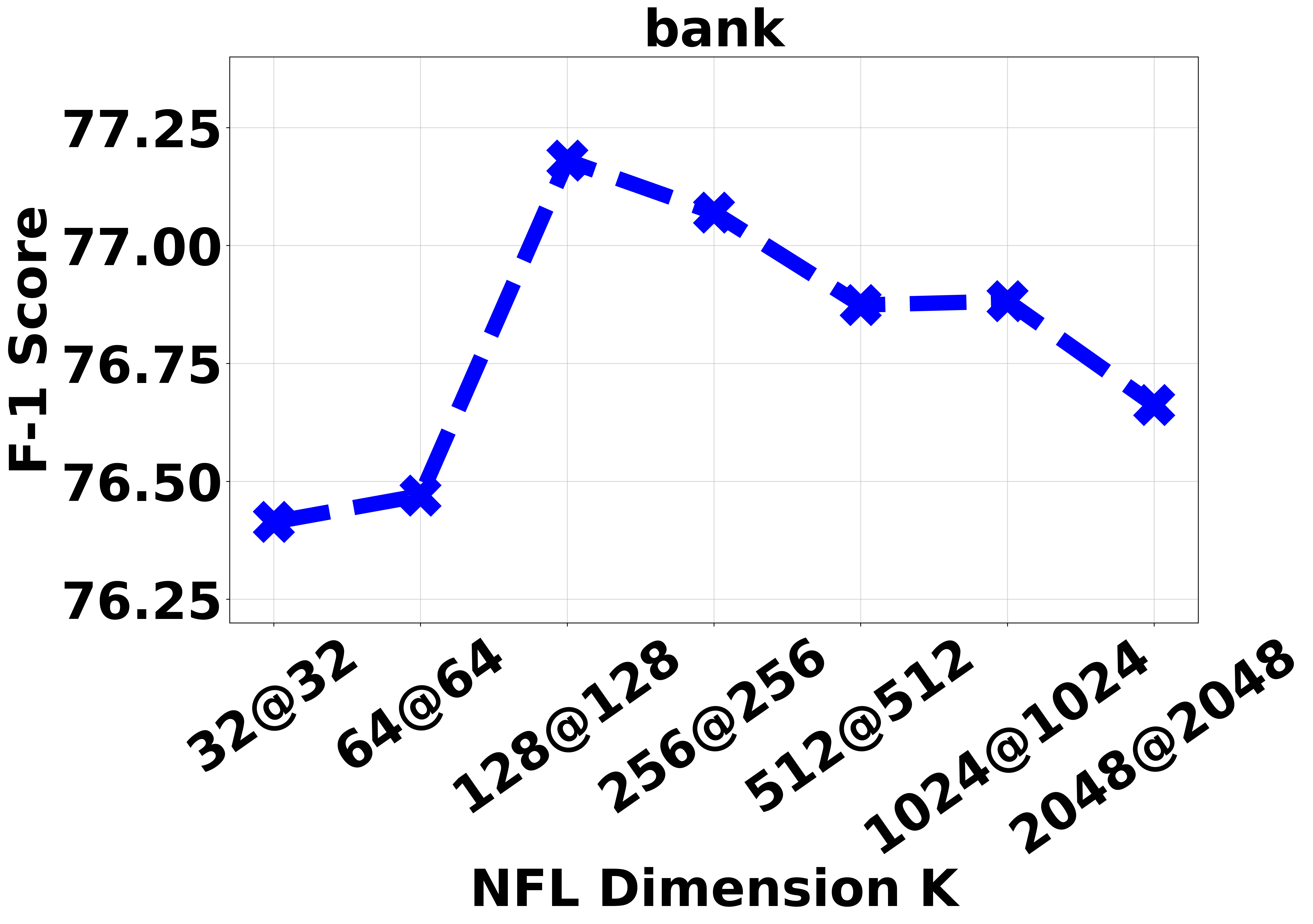
Figure 4: Performance under different Architecture

L2 Regularization $\lambda$. We examine the impact of the L2 regularization weight $\lambda$, which controls NFRL complexity. A larger $\lambda$ reduces model complexity, resulting in fewer and simpler logical rules. We vary $\lambda$ from $1e^{-5}$ to $1e^{-9}$ and show the model’s performance in Figure 5 . The F1 score initially rises and then falls as $\lambda$ increases, indicating that performance improves with an appropriately chosen $\lambda$. Balancing $\lambda$ is essential to avoid overfitting or underfitting and achieve optimal model complexity.

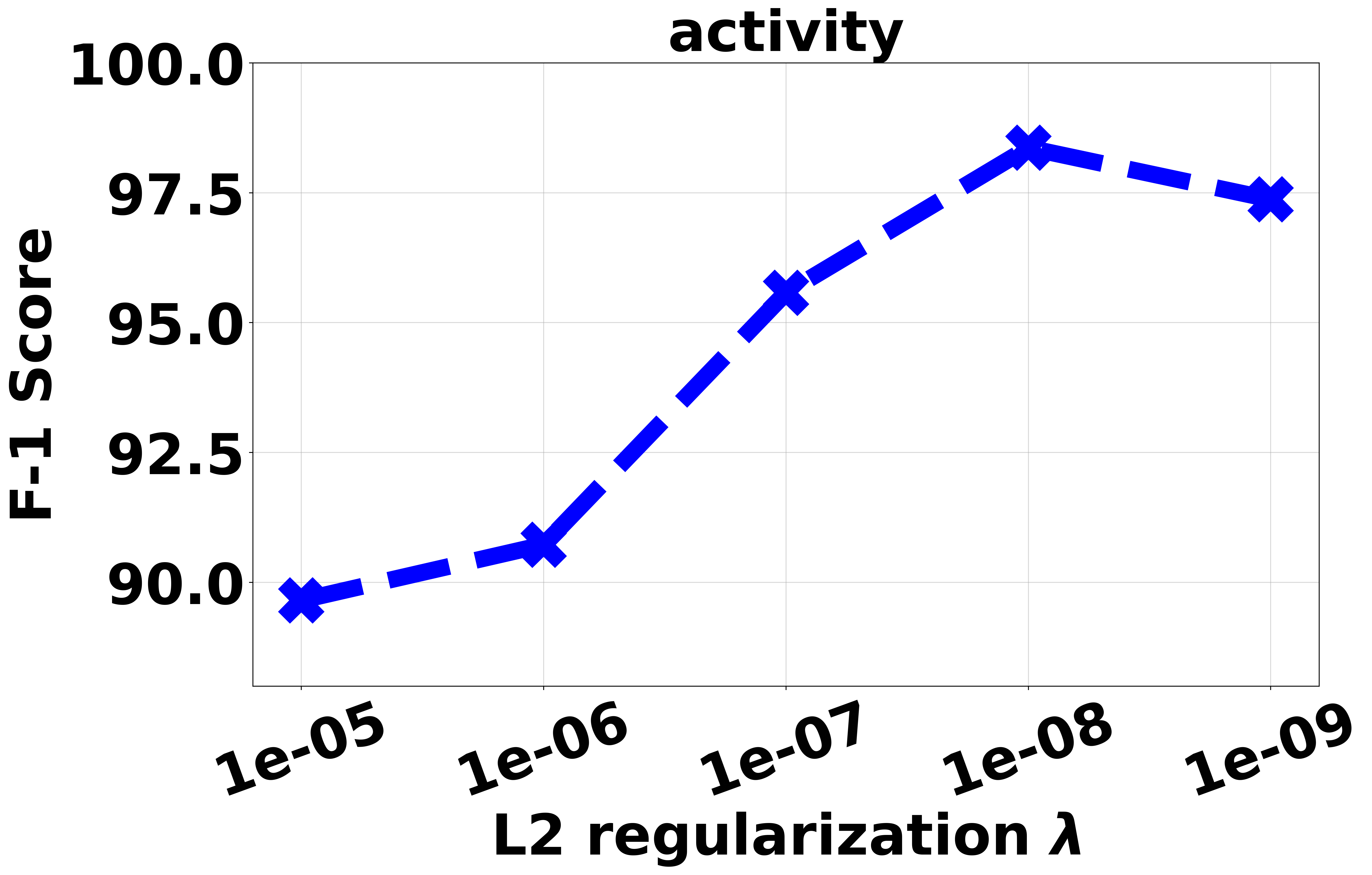
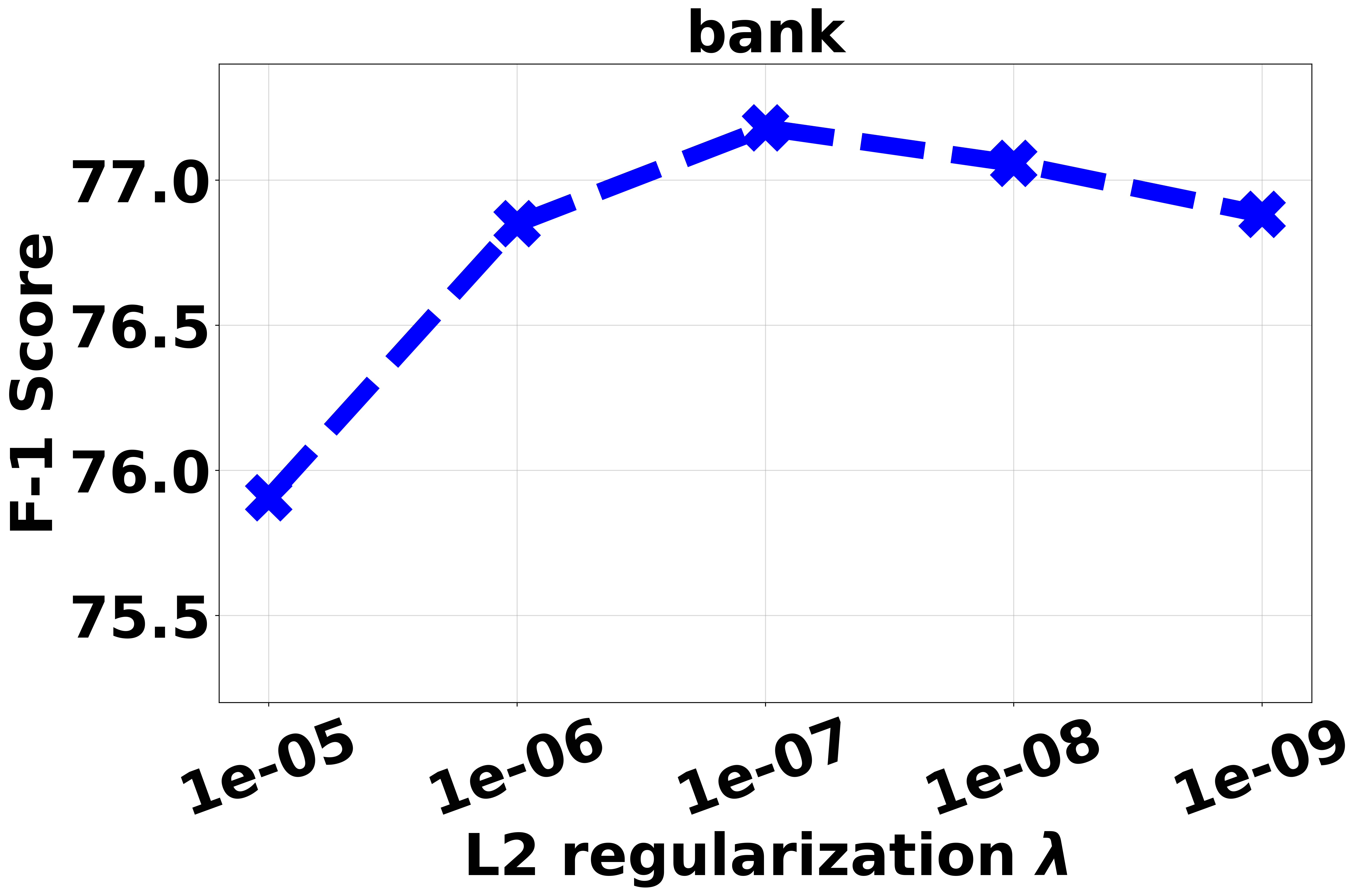
Figure 5: Performance under different L2 regularization

Appendix C Rule Quality

C.1 Rule Quality Metrics

We adopt evaluation metrics including diversity, coverage, and single rule accuracy. We conduct extensive experiments across 10 datasets, as shown in Figure 6, Figure 7 and Figure 8 . NFRL consistently produces rules with superior results: higher accuracy, greater diversity, and lower coverage deviation. This indicates that the rules learned by NFRL are easier to distinguish and exhibit better prediction and generalization power.

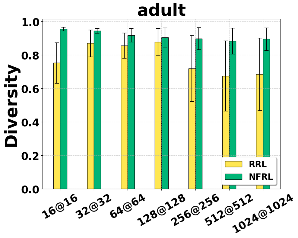
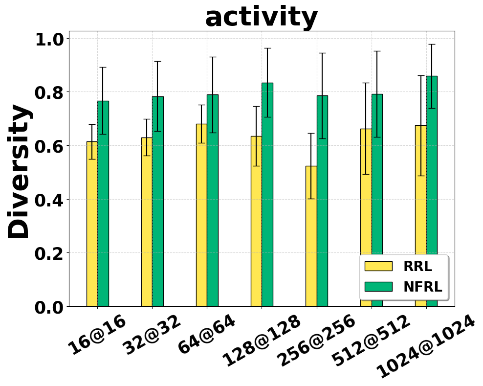
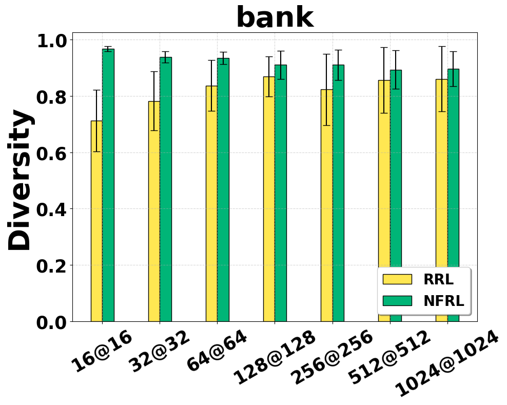
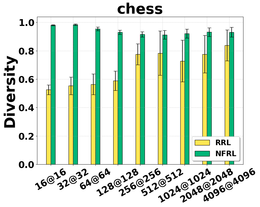
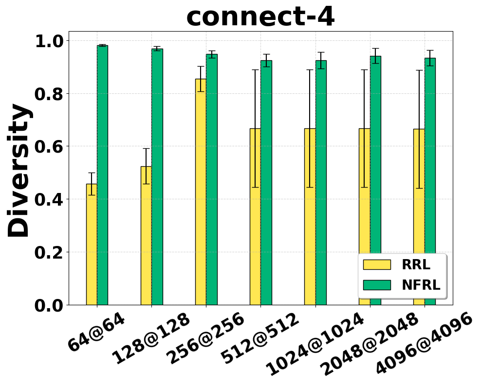
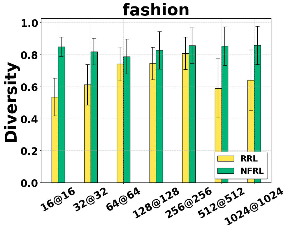
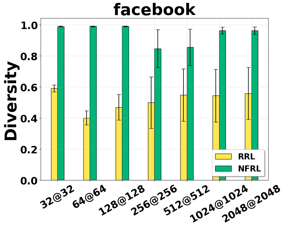
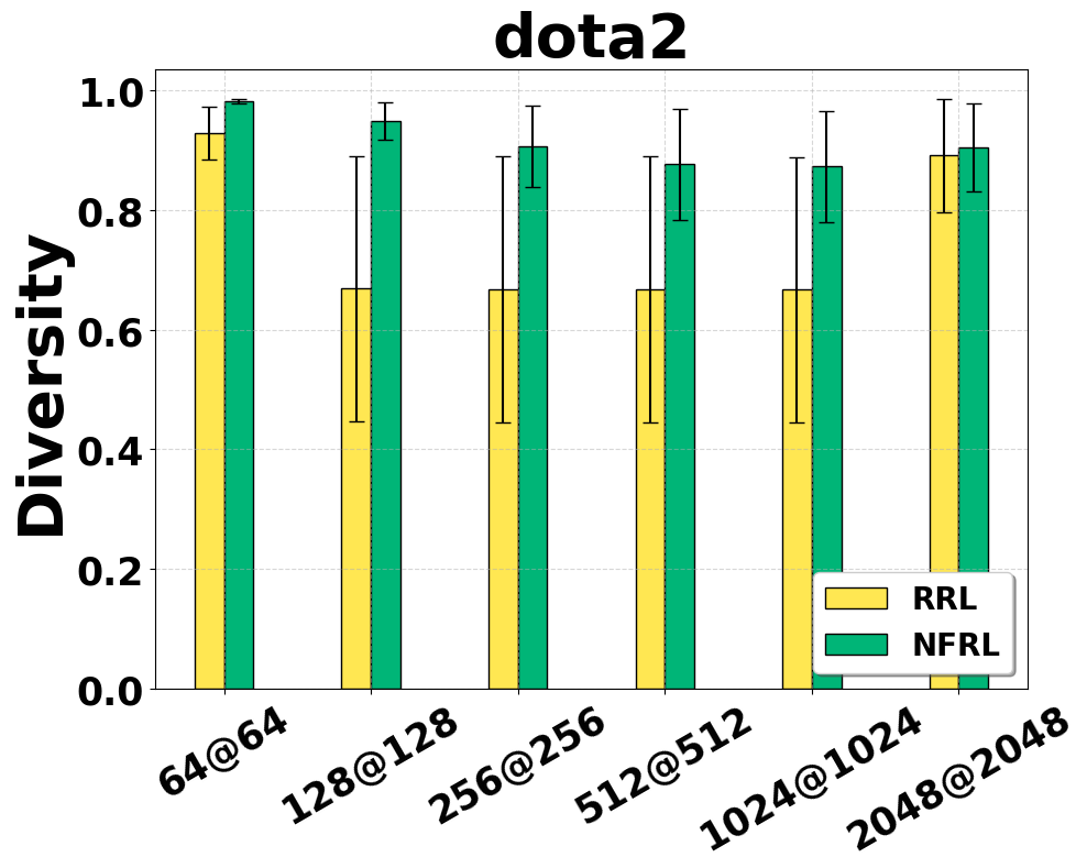
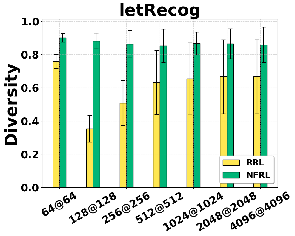
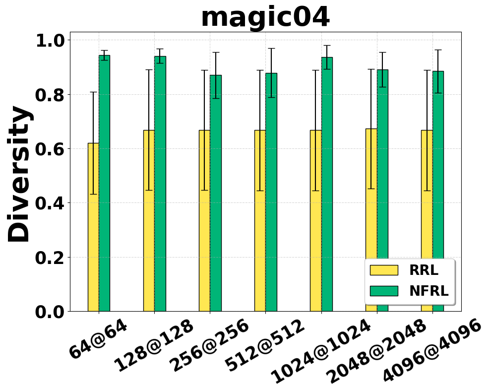
Figure 6: Rule Diversity comparison across different architectures.

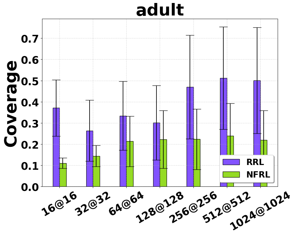
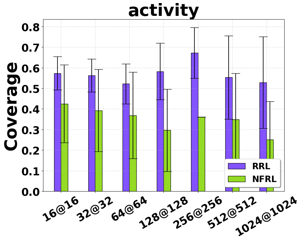
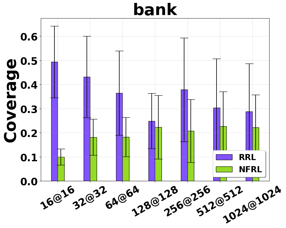
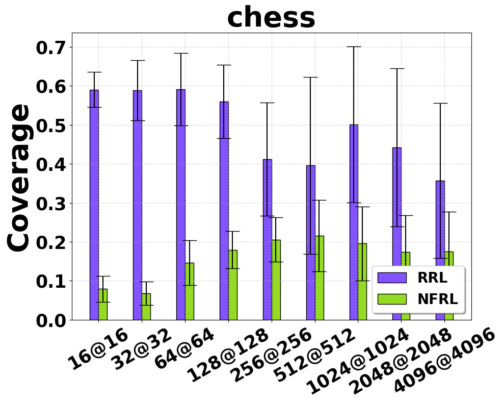
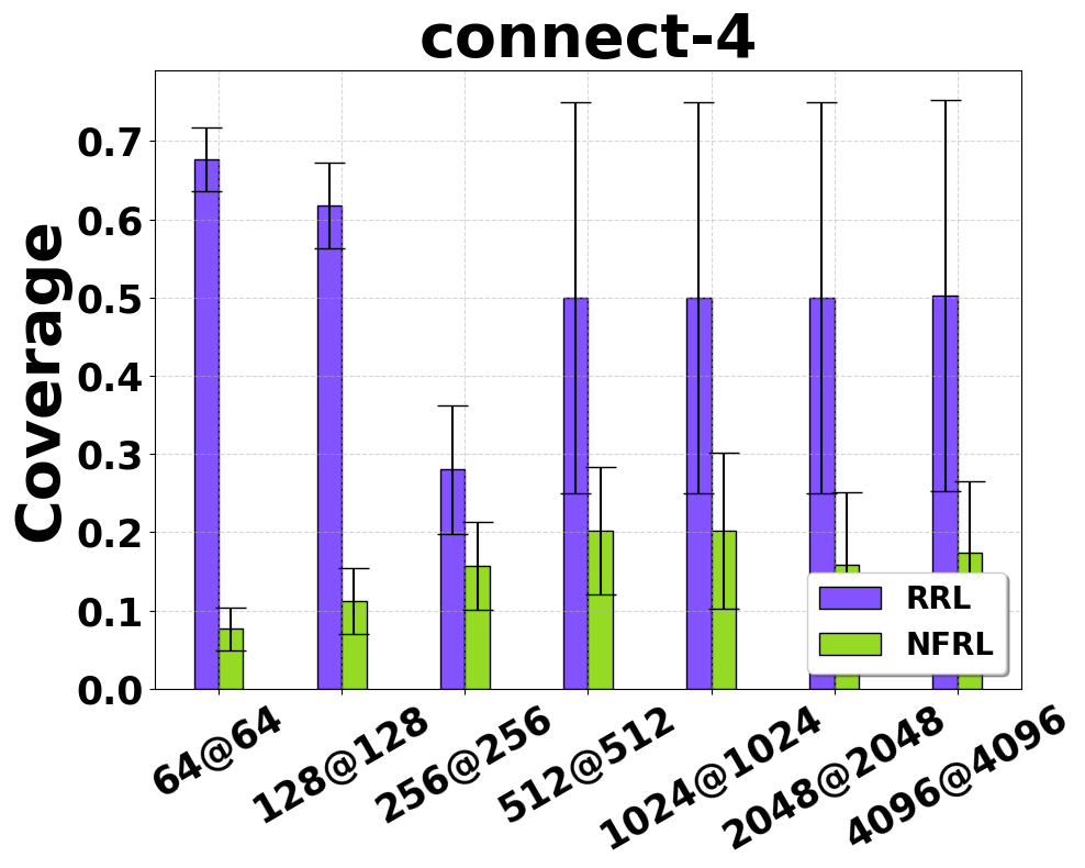
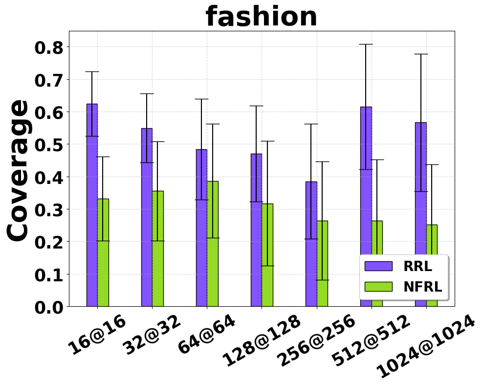
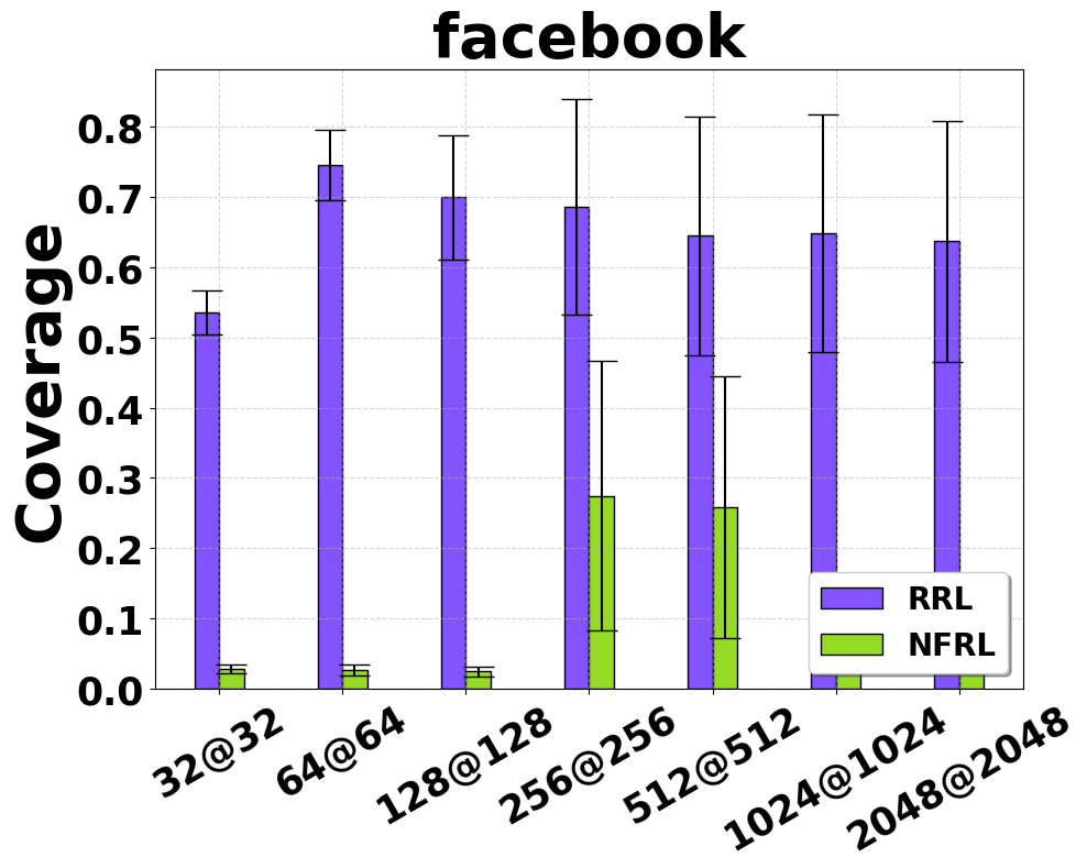
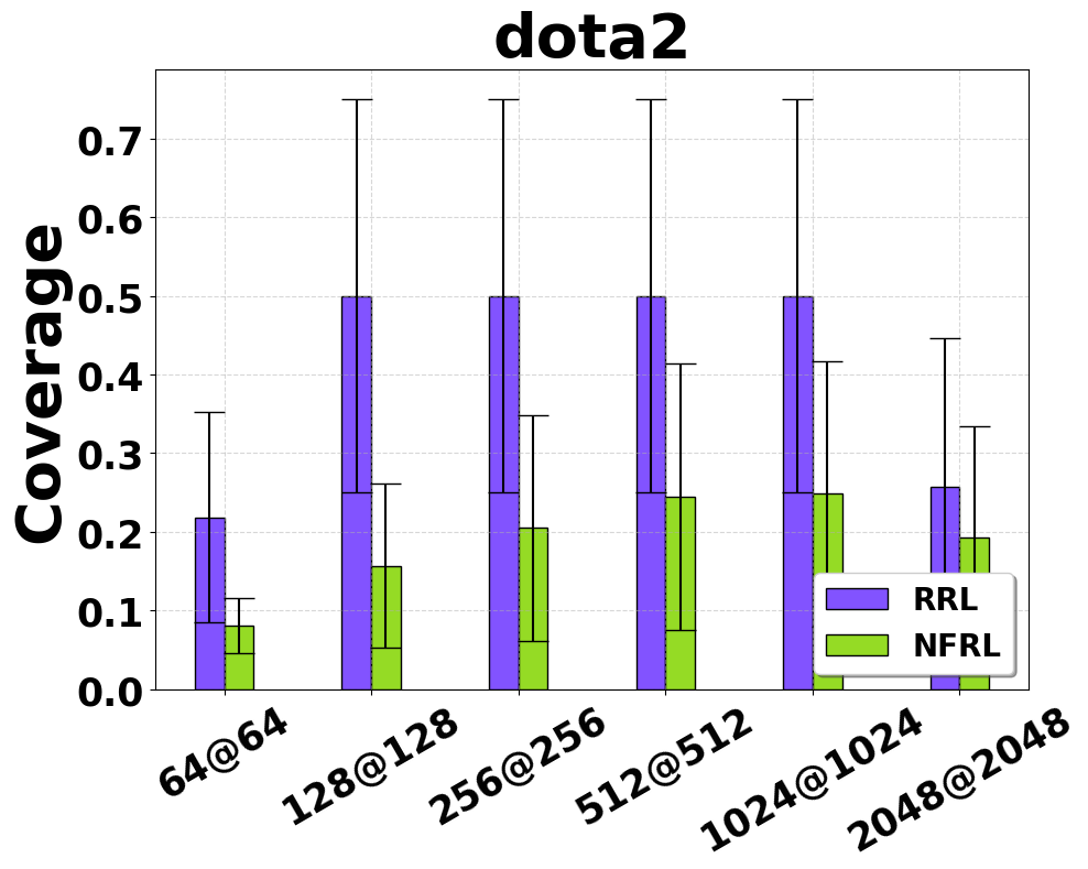
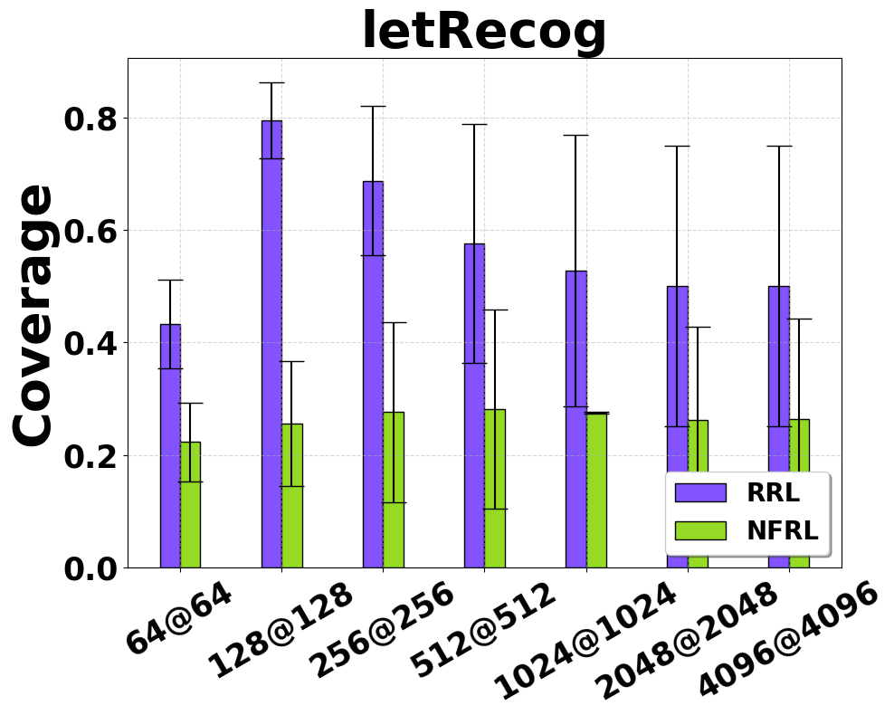
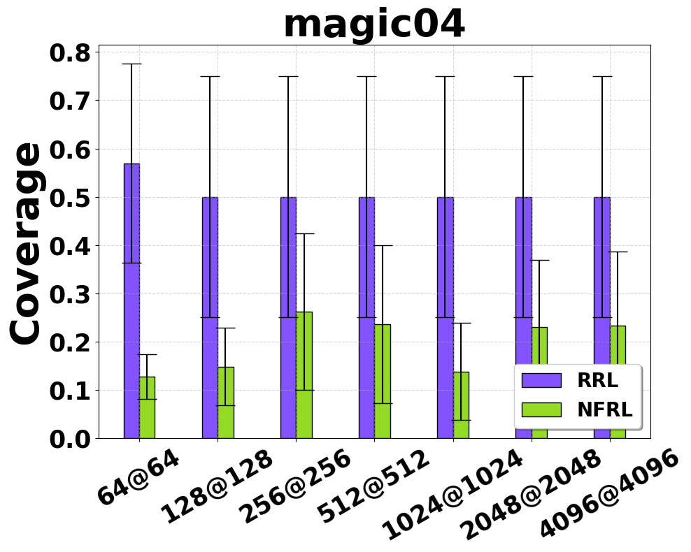
Figure 7: Rule Coverage comparison across different architectures.

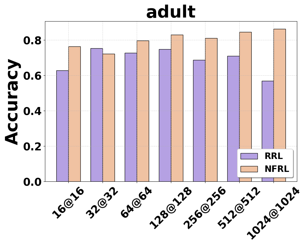
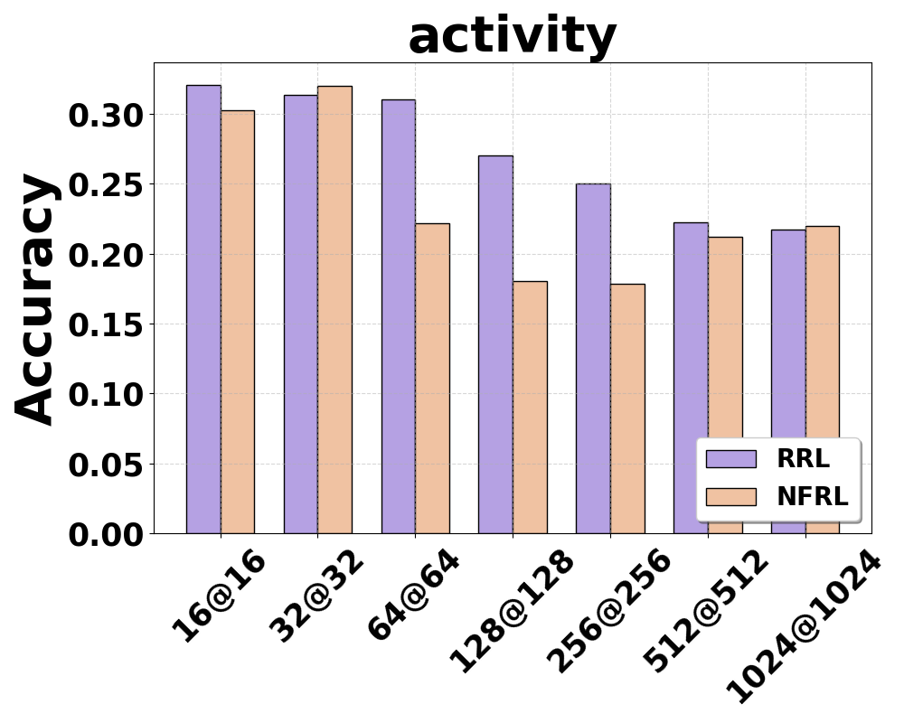
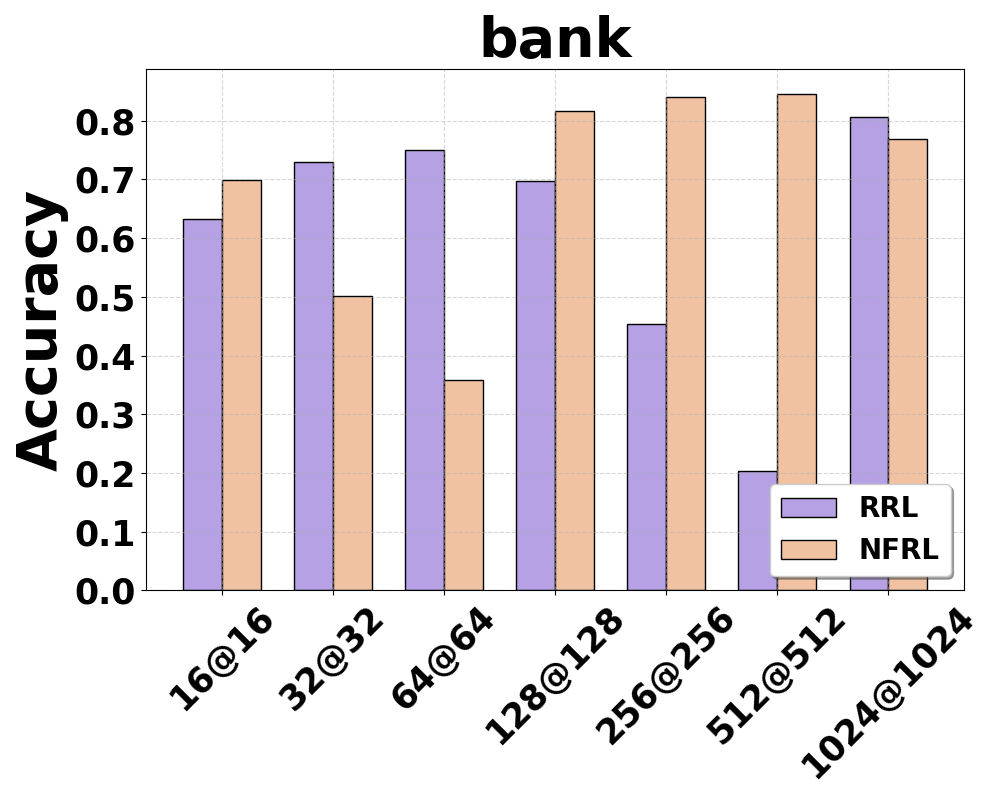
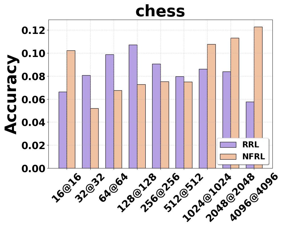
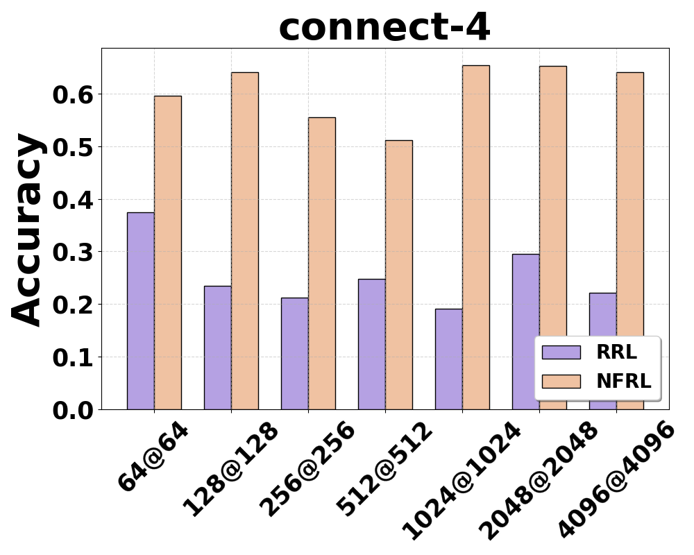
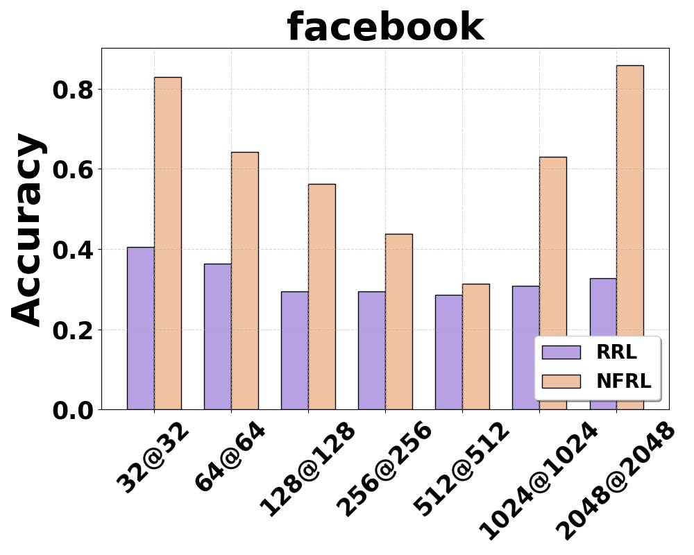
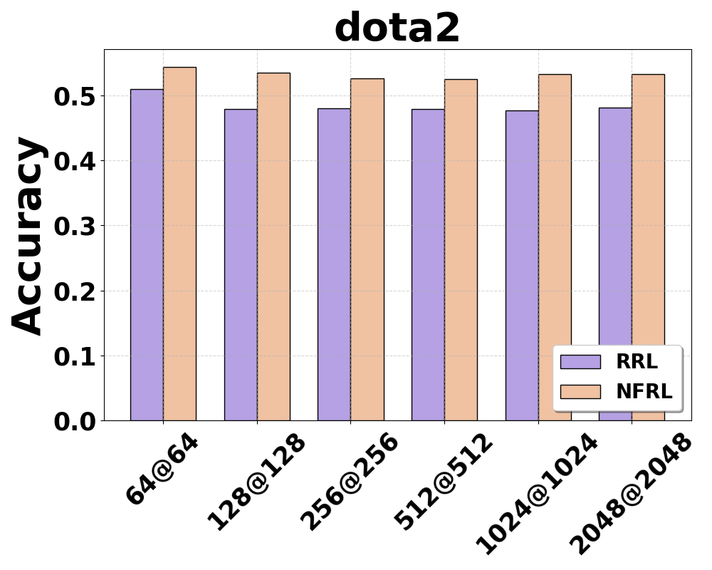
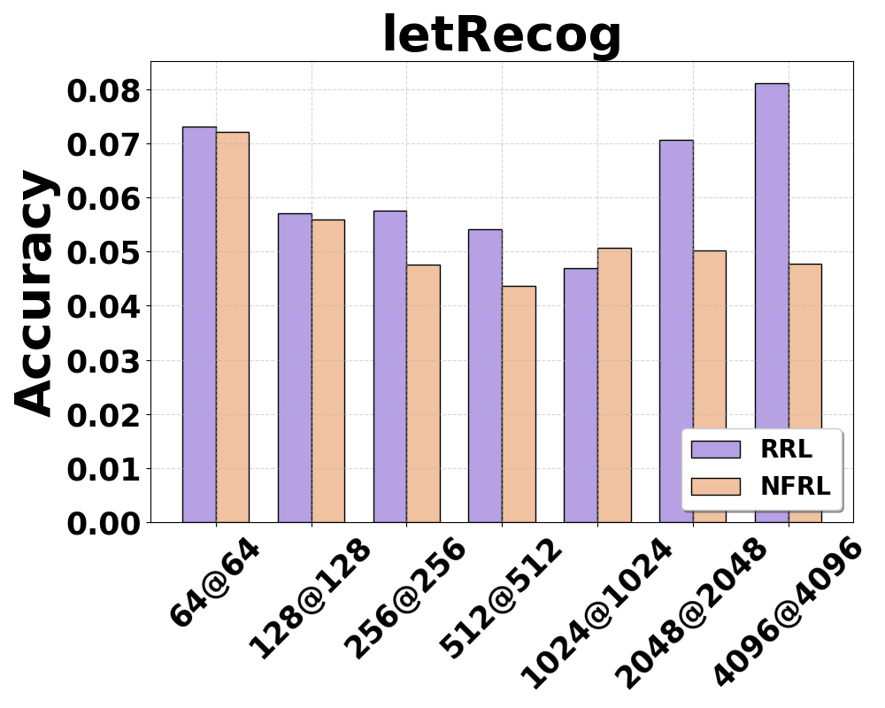
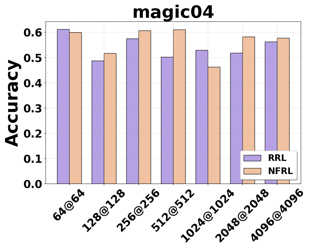
Figure 8: Rule Accuracy comparison across different architectures.

C.2 Simulation Experiment

We are investigating the capability of NFRL in uncovering the underlying data generation processes. Our study includes a comparison with RRL under a naive negation setting, which simply doubles the number of input features, in Table 5. The closer the generated rules are to the ground truth, the better. NFRL consistently outperforms RRL in this regard.

Ground-Truth Rules	Rules_Ours	Rules_RRL
$(x_{1}\lor x_{2})\land\lnot x_{3}$	$x_{1}\land\lnot x_{3}$	$x_{1}\land\lnot x_{2}\land\lnot x_{3}$
	$x_{2}\land\lnot x_{3}$	$x_{1}$
	$x_{1}\land x_{2}\land\lnot x_{3}$	$\lnot x_{3}$
		$x_{2}\land x_{3}$
$x_{1}\lor(\lnot x_{2}\land\lnot x_{3})$	$\lnot x_{2}\land\lnot x_{3}$	$x_{1}$
	$x_{1}$	$x_{2}$
		$x_{1}\lor\lnot x_{2}\land x_{3}$
$x_{1}\land\lnot x_{2}\land x_{3}$	$x_{1}\land\lnot x_{2}\land x_{3}$	$x_{1}\land x_{3}$
		$\lnot x_{2}\lor x_{3}\lor x_{1}$
		$(x_{1}\land x_{3})\land x_{1}$
$x_{1}\lor\lnot x_{2}\lor\lnot x_{3}$	$x_{1}\lor\lnot x_{2}\lor\lnot x_{3}$	$x_{1}\land\lnot x_{3}$
		$\lnot x_{2}\land\lnot x_{3}$

Table 5: Logical rules obtained from NFRL trained on the synthetic dataset.

Appendix D Efficiency

We evaluate learning efficiency by the number and length of learned rules across all datasets, as shown in Figure 9 and Figure 10, respectively. Figure 9 presents scatter plots of F1 score against log(#edges) across 10 datasets. The boundary connecting the results of different NFRL architectures separates the upper left corner from the best baseline methods. This indicates that NFRL consistently learns fewer rules while achieving high prediction accuracy across various scenarios. The average length of rules in NFRL trained on different datasets is shown in Figure 10. The average rule length is less than 6 for all datasets except fashion and facebook, which are unstructured datasets and have more complex features. These results indicate that the rules learned by NFRL are generally easy to understand across different scenarios.

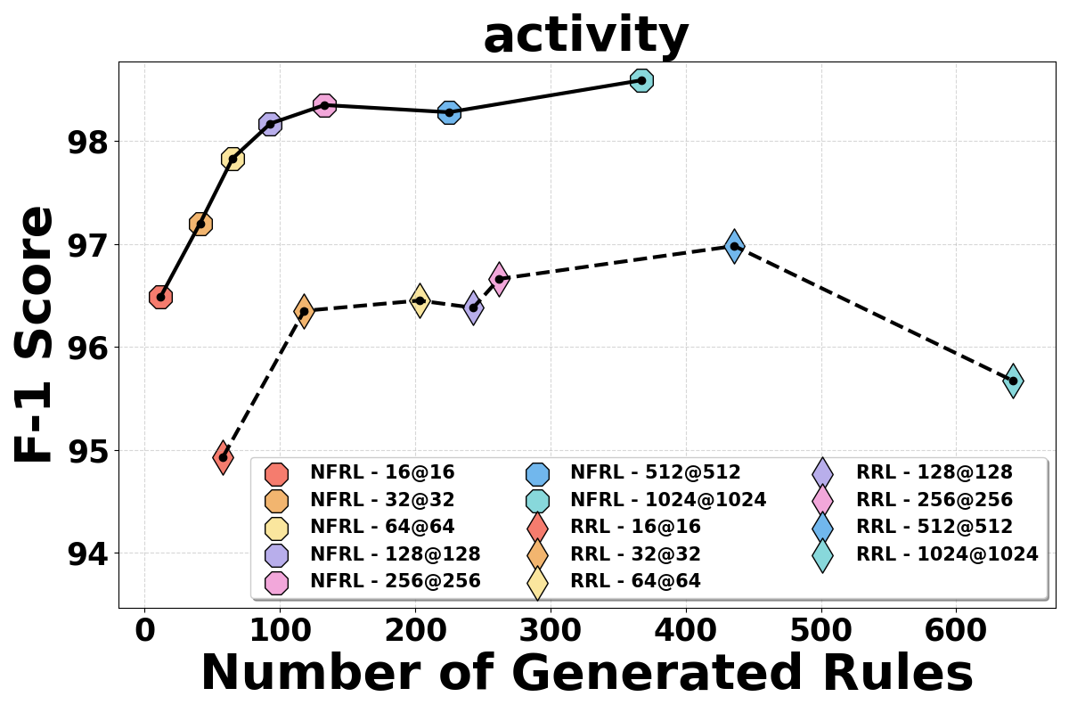
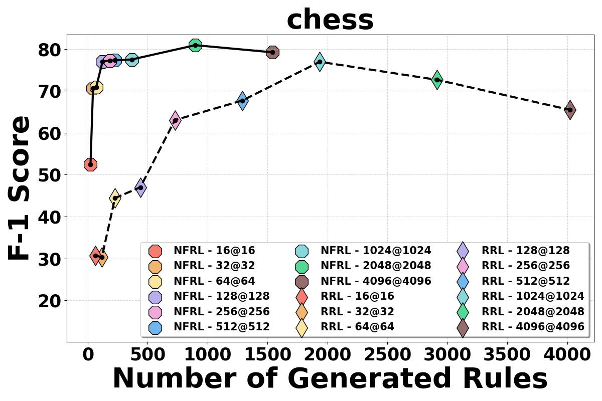
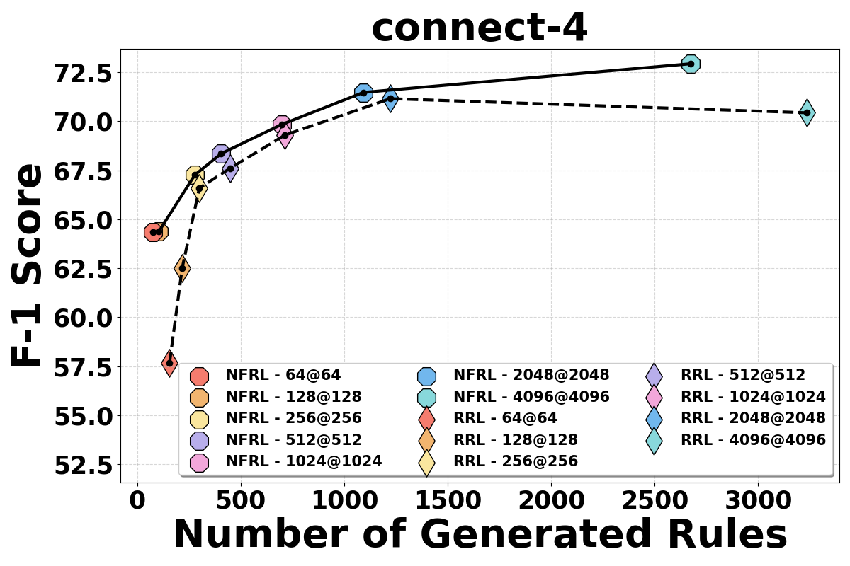
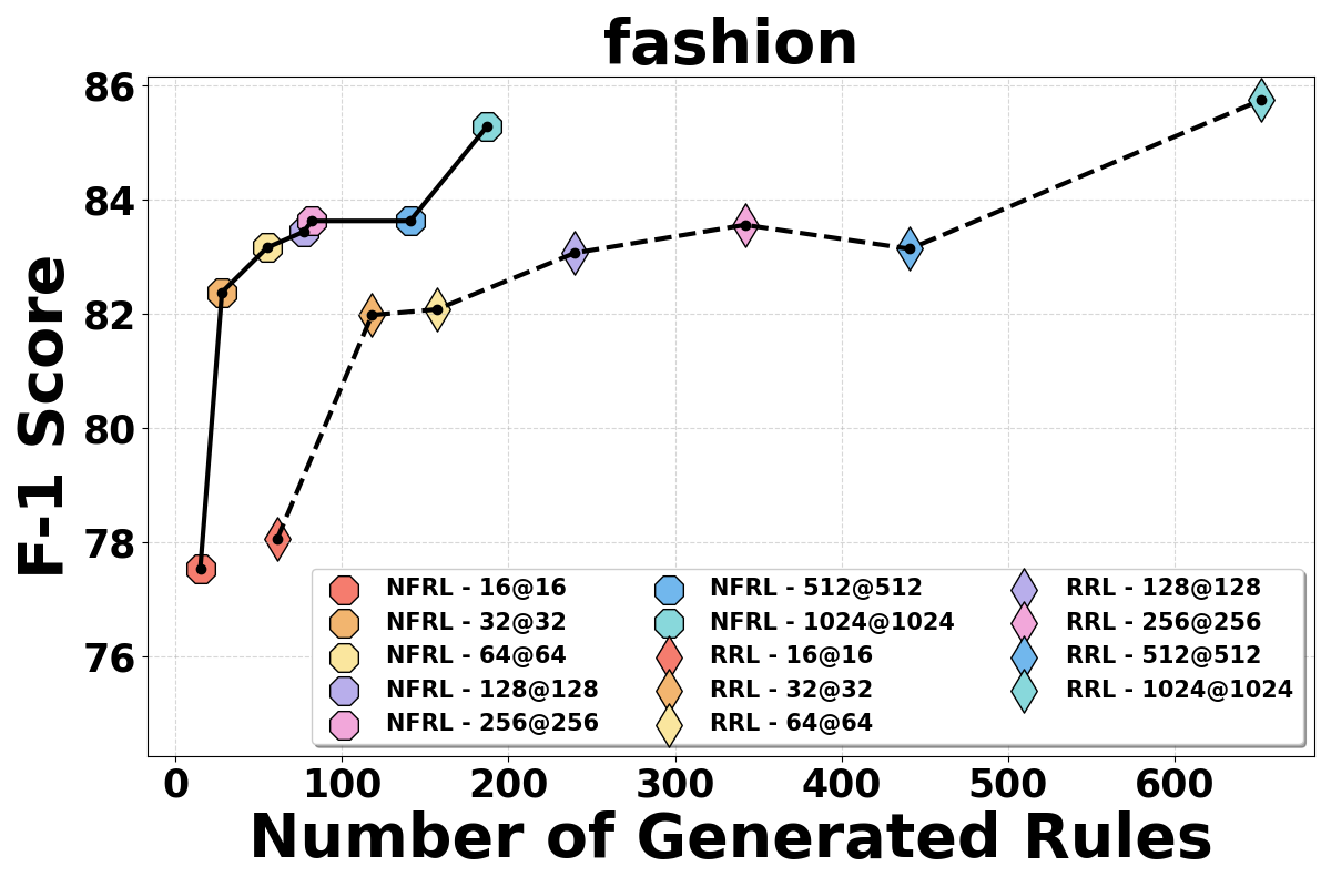
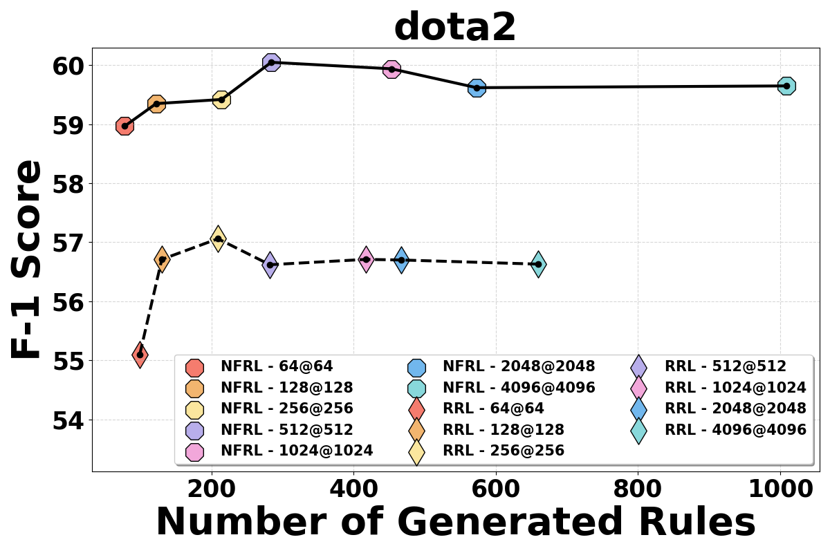
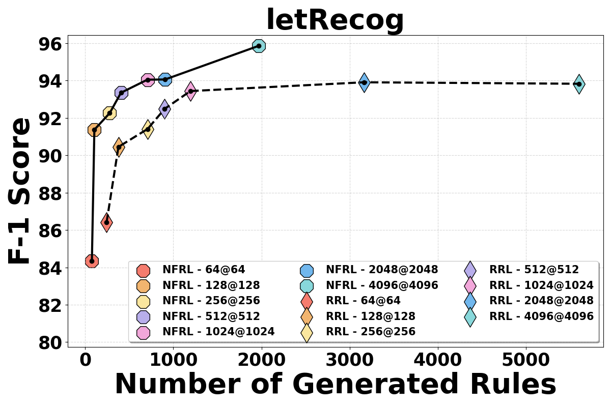
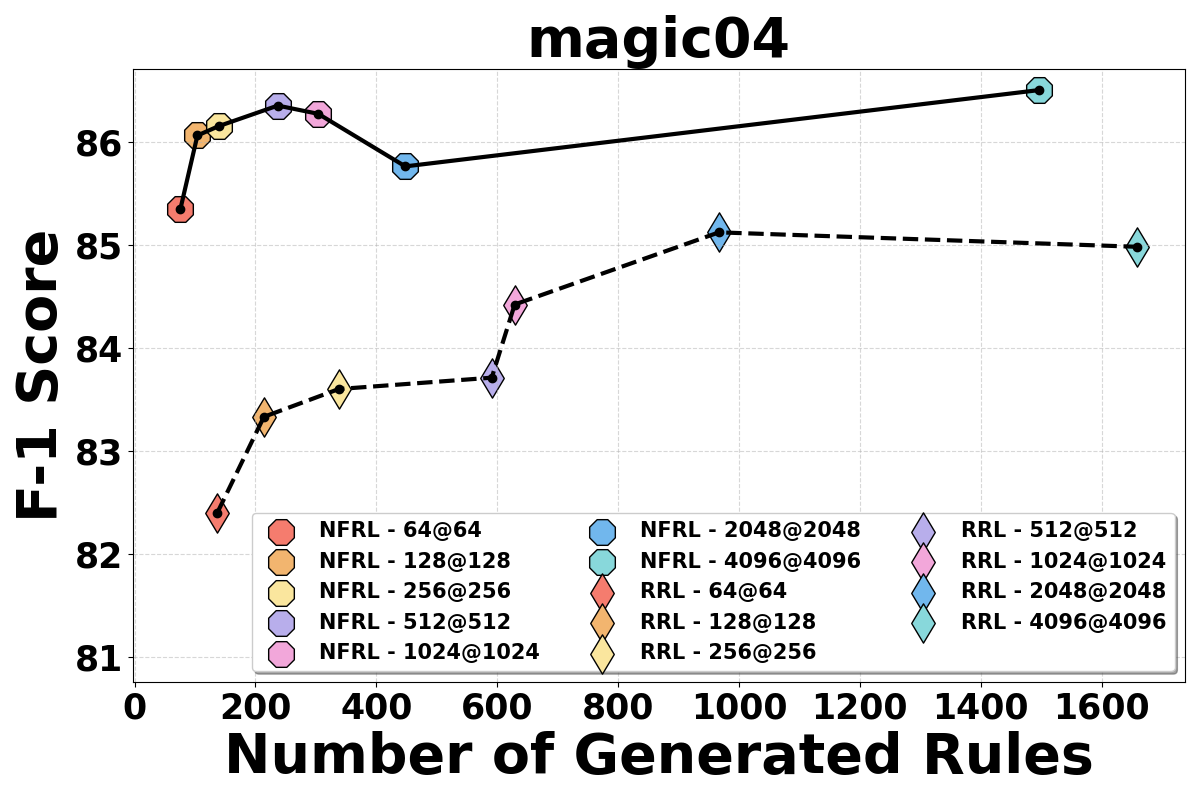
Figure 9: Rule Number comparison across different architectures.

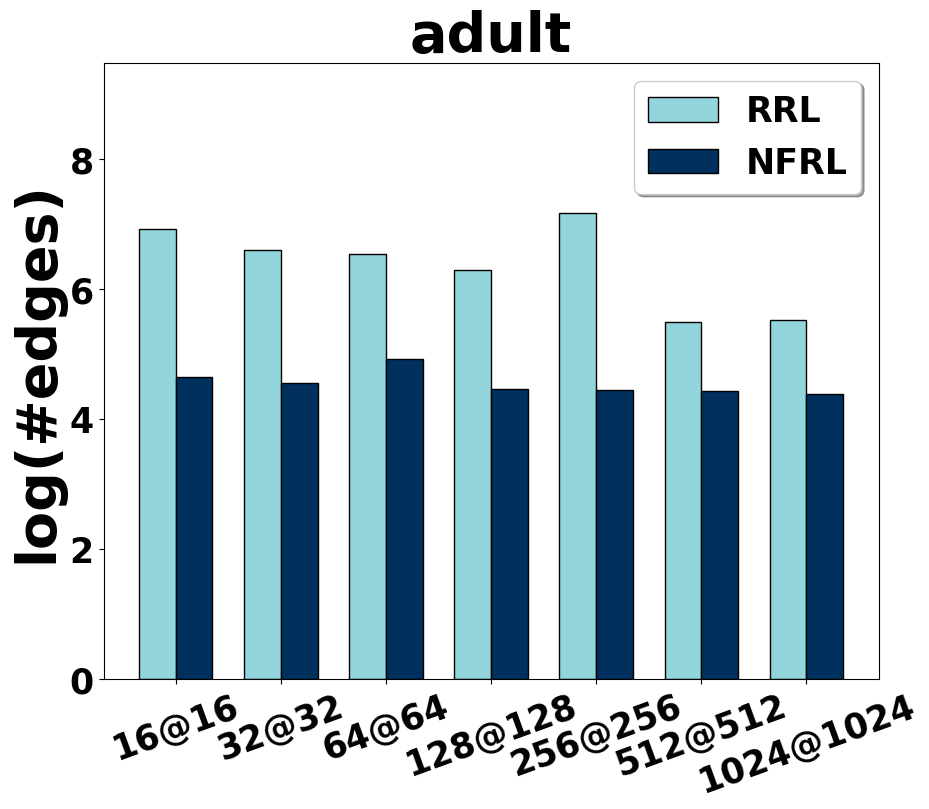
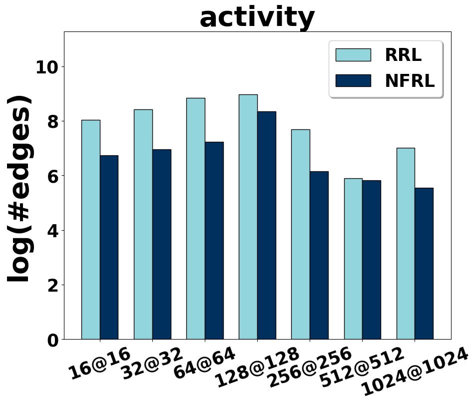
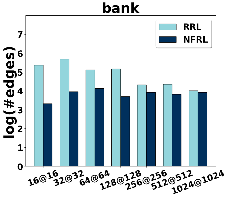
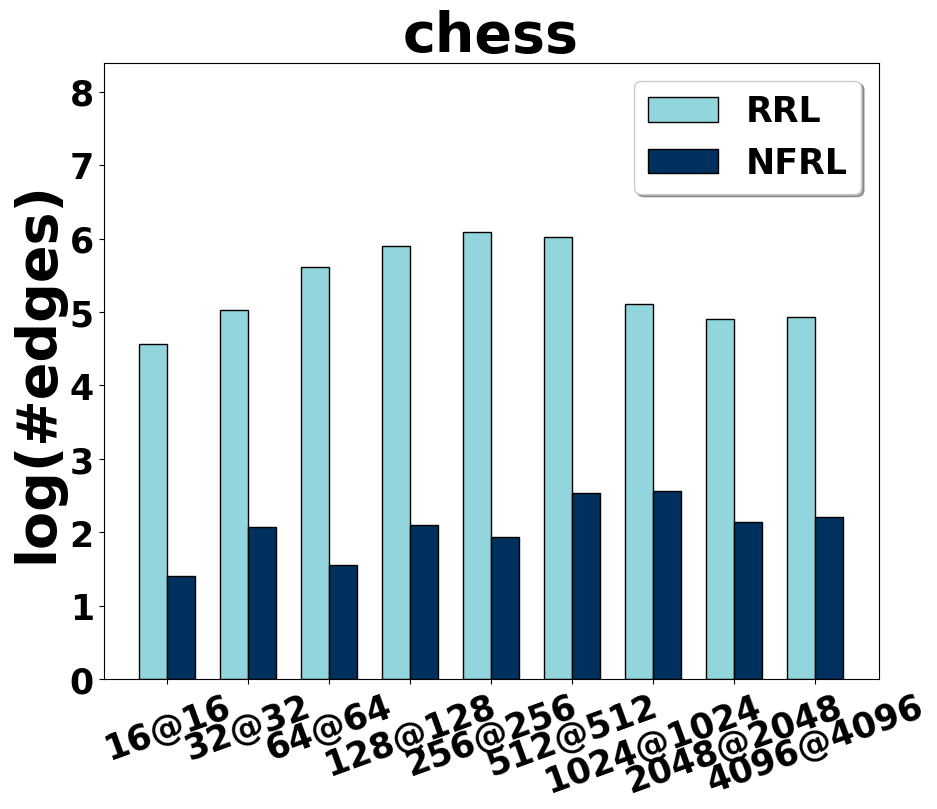
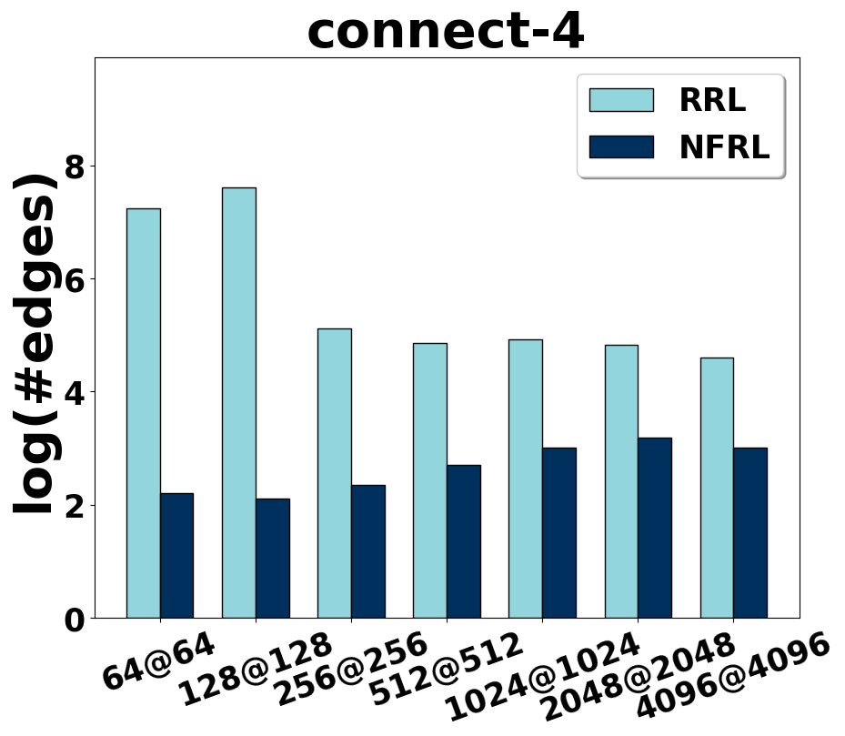
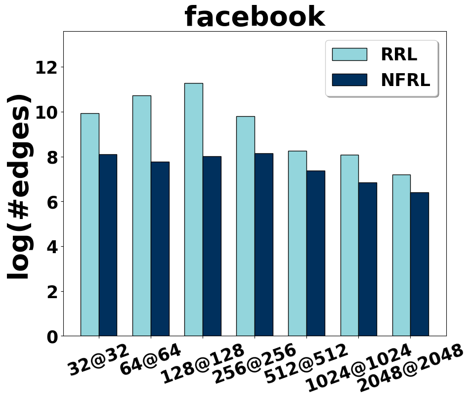
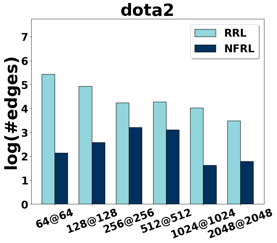
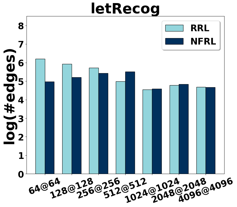
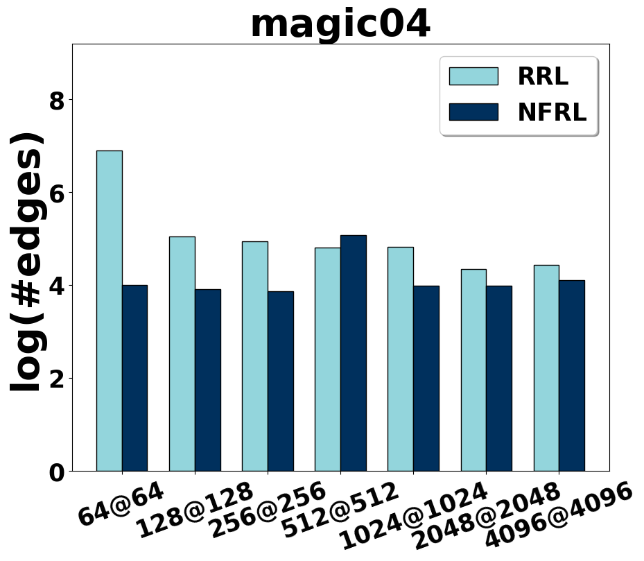
Figure 10: Rule Length comparison across different architectures.

Appendix E Ablation Study

Negative Layer and NFC. To demonstrate the effectiveness of the Negation Layer and Normal Form Constraint (NFC), we compare NFRL trained with and without these components. The Negation Layer supports negation operations in learned rules for functional completeness, while NFC narrows the search space for learning connections between logical layers, both enhancing model performance.Table 6 shows F1 scores for NFRL and its variants on a small dataset (bank) and a large dataset (activity). The decreases in F1 scores when the Negation Layer and NFC are removed underscore their importance.

Additionally, NFC enhances learning efficiency. With all other factors constant, we compare the training time for NFRL with and without NFC. As shown in Table 7, NFC reduces training time by 11.22% for the activity dataset and 25% for the bank dataset, highlighting its necessity and importance.

Binning Function. We study how NFRL performs with different binning functions. We consider four methods: RanInt Wang et al. [2021] (the default in this paper introduced in Section 3.2), KInt Dougherty et al. [1995], EntInt Wang et al. [2020], and AutoInt Zhang et al. [2023].

Table 8 shows the F1 scores of NFRL with different binning functions. NFRL demonstrates strong flexibility, with RanInt achieving the best performance. The randomness in interval selection introduces stochastic diversity, helping to prevent overfitting. Its computational efficiency and intuitive design are also advantageous. In contrast, KInt clusters features based solely on feature values, neglecting the target variable, which can result in less effective bins. EntInt forms bins that minimize entropy using label data, potentially enhancing predictive accuracy. AutoInt offers adaptability but is computationally intensive, posing optimization challenges in practice.

	activity	bank
w/o Negation Layer	97.68	76.92
w/o NFC	97.81	76.36
Ours	98.37	77.18

Table 6: F1 Score(%) of NFRL and its variants.

	activity	bank
w/o NFC	1h38min9s	1h24min50s
Ours	1h27min3s	1h3min56s

Table 7: Training time of NFRL with and without NFC.

	activity	bank
KInt	92.71	74.37
EntInt	97.09	77.02
AutoInt	95.62	75.59
RanInt	98.80	77.18

Table 8: F1 Score(%) of NFRL with different feature binning methods.

Appendix F Gradient vanishing

Despite the high interpretability of discrete logical layers, training them is challenging due to their discrete parameters and non-differentiable structures. This challenge is addressed by drawing inspiration from the training methods used in binary neural networks, which involve searching for discrete solutions within a continuous space.  Wang et al. [2021] leverages the logical activation functions proposed by Payani and Fekri [2019] in RRL:

$$AND(h,W_{conn}^{i})=\prod_{j=1}^{n}F_{c}(h_{j},W_{i,j})$$ (7)

$$OR(h,W_{conn}^{i})=1-\prod_{j=1}^{n}(1-F_{d}(h_{j},W_{i,j}))$$ (8)

where $F_{c}(h,w)=1-w(1-h)$ and $F_{d}(h,w)=h\cdot w$.

If $\mathbf{h}$ and $W_{i}$ are both binary vectors, then $\text{Conj}(\mathbf{h},W_{i})=\land_{W_{i,j}=1}h_{j}$ and $\text{Disj}(\mathbf{h},W_{i})=\lor_{W_{i,j}=1}h_{j}$. $F_{c}(\mathbf{h},W)$ and $F_{d}(\mathbf{h},W)$ decide how much $h_{j}$ would affect the operation according to $W_{i,j}$. After using continuous weights and logical activation functions, the AND and OR operators, denoted by $R$ and $S$, are defined as follows:

$$r_{i}^{(l)}=AND(u^{(l-1)},W_{i}^{(l,0)})$$ (9)

$$s_{i}^{(l)}=OR(u^{(l-1)},W_{i}^{(l,1)})$$ (10)

Although the whole logical layer becomes differentiable by applying this continuous relaxation, the above functions are not compatible with NFRL. In this setting, the output of the node $h\in[0,1]$ conflicts with our binarized setting, where all logical parameters are either $-1$ or $+1$. This not only breaks the inherently discrete nature of NFRL but also suffers from the serious vanishing gradient problem. The reason can be found by analyzing the partial derivative of each node with respect to its directly connected weights and with respect to its directly connected nodes as follows:

$$\frac{\partial r}{\partial W_{i,j}}=(u_{j}^{(l-1)}-1)\cdot\prod_{k\neq j}F_{c}(u_{k}^{(l-1)},W_{i,k}^{(l,0)})$$ (11)

$$\frac{\partial r}{\partial u_{j}^{(l-1)}}=W_{i,j}^{(l,0)}\cdot\prod_{k\neq j}F_{c}(u_{k}^{(l-1)},W_{i,k}^{(l,0)})$$ (12)

Since $u_{j}^{(l-1)}$ and $W_{i,k}^{(l,0)}$ fall within the range of 0 to 1, the values of $F_{c}(\cdot)$ also lie within this range. If the number of inputs is large and most $F_{c}(\cdot)$ are not 1, the gradient tends toward 0 due to multiplications. Additionally, in the discrete setting, only when $u_{j}^{(l-1)}$ and $1-F_{d}(\cdot)$ are all 1, can the gradient be non-zero, which is quite rare in practice.

References

- Angelov et al. [2021] Plamen P Angelov, Eduardo A Soares, Richard Jiang, Nicholas I Arnold, and Peter M Atkinson. Explainable artificial intelligence: an analytical review. Wiley Interdisciplinary Reviews: Data Mining and Knowledge Discovery, 11(5):e1424, 2021.
- Rudin [2019] Cynthia Rudin. Stop explaining black box machine learning models for high stakes decisions and use interpretable models instead, 2019. URL https://arxiv.org/abs/1811.10154.
- Setzu et al. [2021] Mattia Setzu, Riccardo Guidotti, Anna Monreale, Franco Turini, Dino Pedreschi, and Fosca Giannotti. Glocalx - from local to global explanations of black box ai models. Artificial Intelligence, 294:103457, May 2021. ISSN 0004-3702. doi:10.1016/j.artint.2021.103457. URL http://dx.doi.org/10.1016/j.artint.2021.103457.
- Lundberg et al. [2020] Scott M Lundberg, Gabriel Erion, Hugh Chen, Alex DeGrave, Jordan M Prutkin, Bala Nair, Ronit Katz, Jonathan Himmelfarb, Nisha Bansal, and Su-In Lee. From local explanations to global understanding with explainable ai for trees. Nature machine intelligence, 2(1):56–67, 2020.
- Molnar [2020] Christoph Molnar. Interpretable machine learning. Lulu. com, 2020.
- Yin and Han [2003] Xiaoxin Yin and Jiawei Han. Cpar: Classification based on predictive association rules. In Proceedings of the 2003 SIAM international conference on data mining, pages 331–335. SIAM, 2003.
- Frank and Witten [1998] Eibe Frank and Ian H Witten. Generating accurate rule sets without global optimization. 1998.
- Cohen [1995] William W Cohen. Fast effective rule induction. In Machine learning proceedings 1995, pages 115–123. Elsevier, 1995.
- Wang et al. [2020] Zhuo Wang, Wei Zhang, Ning Liu, and Jianyong Wang. Transparent classification with multilayer logical perceptrons and random binarization, 2020.
- Wang et al. [2021] Zhuo Wang, Wei Zhang, Ning Liu, and Jianyong Wang. Scalable rule-based representation learning for interpretable classification, 2021.
- Quinlan [2014] J Ross Quinlan. C4. 5: programs for machine learning. Elsevier, 2014.
- Yang et al. [2017] Hongyu Yang, Cynthia Rudin, and Margo Seltzer. Scalable bayesian rule lists. In International conference on machine learning, pages 3921–3930. PMLR, 2017.
- Angelino et al. [2018] Elaine Angelino, Nicholas Larus-Stone, Daniel Alabi, Margo Seltzer, and Cynthia Rudin. Learning certifiably optimal rule lists for categorical data. Journal of Machine Learning Research, 18(234):1–78, 2018.
- Breiman [2017] Leo Breiman. Classification and regression trees. Routledge, 2017.
- Mooney [1995] Raymond J Mooney. Encouraging experimental results on learning cnf. Machine Learning, 19:79–92, 1995.
- Dries et al. [2009] Anton Dries, Luc De Raedt, and Siegfried Nijssen. Mining predictive k-cnf expressions. IEEE Transactions on Knowledge and Data Engineering, 22(5):743–748, 2009.
- Jain et al. [2021] Arcchit Jain, Clément Gautrais, Angelika Kimmig, and Luc De Raedt. Learning cnf theories using mdl and predicate invention. In IJCAI, pages 2599–2605, 2021.
- Beck et al. [2023] Florian Beck, Johannes Fürnkranz, and Van Quoc Phuong Huynh. Layerwise learning of mixed conjunctive and disjunctive rule sets. In International Joint Conference on Rules and Reasoning, pages 95–109. Springer, 2023.
- Sverdlik [1992] William Sverdlik. Dynamic version spaces in machine learning. Wayne State University, 1992.
- Hong and Tsang [1997] Tzung-Pai Hong and Shian-Shyong Tsang. A generalized version space learning algorithm for noisy and uncertain data. IEEE Transactions on Knowledge and Data Engineering, 9(2):336–340, 1997.
- S. [1969] MICHALSKI R. S. On the quasi-minimal solution of the general covering problem. Proceedings of the 5th International Symposium on Information Processing, 3:125–128, 1969. URL https://cir.nii.ac.jp/crid/1571135649817801472.
- Michalski [1973] Ryszard S. Michalski. Aqval/1–computer implementation of a variable-valued logic system vl1 and examples of its application to pattern recognition. In International Joint Conference on Artificial Intelligence, 1973. URL https://api.semanticscholar.org/CorpusID:60492559.
- Pagallo and Haussler [1990] Giulia Pagallo and David Haussler. Boolean feature discovery in empirical learning. Machine Learning, 5:71–99, 1990. URL https://api.semanticscholar.org/CorpusID:5661437.
- Clark and Niblett [1989] Peter Clark and Tim Niblett. The cn2 induction algorithm. Mach. Learn., 3(4):261–283, mar 1989. ISSN 0885-6125. doi:10.1023/A:1022641700528. URL https://doi.org/10.1023/A:1022641700528.
- Quinlan [1990] J. Ross Quinlan. Learning logical definitions from relations. Machine Learning, 5:239–266, 1990. URL https://api.semanticscholar.org/CorpusID:6746439.
- Loh [2011] Wei-Yin Loh. Classification and regression trees. Wiley interdisciplinary reviews: data mining and knowledge discovery, 1(1):14–23, 2011.
- Ke et al. [2017] Guolin Ke, Qi Meng, Thomas Finley, Taifeng Wang, Wei Chen, Weidong Ma, Qiwei Ye, and Tie-Yan Liu. Lightgbm: A highly efficient gradient boosting decision tree. Advances in neural information processing systems, 30, 2017.
- Breiman [2001] Leo Breiman. Random forests. Machine learning, 45:5–32, 2001.
- Irsoy et al. [2012] Ozan Irsoy, Olcay Taner Yıldız, and Ethem Alpaydın. Soft decision trees. In Proceedings of the 21st international conference on pattern recognition (ICPR2012), pages 1819–1822. IEEE, 2012.
- Letham et al. [2015] Benjamin Letham, Cynthia Rudin, Tyler H. McCormick, and David Madigan. Interpretable classifiers using rules and bayesian analysis: Building a better stroke prediction model. The Annals of Applied Statistics, 9(3), September 2015. ISSN 1932-6157. doi:10.1214/15-aoas848. URL http://dx.doi.org/10.1214/15-AOAS848.
- Wang et al. [2017] Tong Wang, Cynthia Rudin, Finale Doshi-Velez, Yimin Liu, Erica Klampfl, and Perry MacNeille. A bayesian framework for learning rule sets for interpretable classification. The Journal of Machine Learning Research, 18(1):2357–2393, 2017.
- Yu et al. [2023] Lu Yu, Meng Li, Ya-Lin Zhang, Longfei Li, and Jun Zhou. Finrule: Feature interactive neural rule learning. In Proceedings of the 32nd ACM International Conference on Information and Knowledge Management, pages 3020–3029, 2023.
- Liu et al. [1998] Bing Liu, Wynne Hsu, and Yiming Ma. Integrating classification and association rule mining. In Proceedings of the fourth international conference on knowledge discovery and data mining, pages 80–86, 1998.
- Li et al. [2001] Wenmin Li, Jiawei Han, and Jian Pei. Cmar: Accurate and efficient classification based on multiple class-association rules. In Proceedings 2001 IEEE international conference on data mining, pages 369–376. IEEE, 2001.
- Lakkaraju et al. [2016] Himabindu Lakkaraju, Stephen H Bach, and Jure Leskovec. Interpretable decision sets: A joint framework for description and prediction. In Proceedings of the 22nd ACM SIGKDD international conference on knowledge discovery and data mining, pages 1675–1684, 2016.
- Chen and Guestrin [2016] Tianqi Chen and Carlos Guestrin. Xgboost: A scalable tree boosting system. In Proceedings of the 22nd acm sigkdd international conference on knowledge discovery and data mining, pages 785–794, 2016.
- Frosst and Hinton [2017] Nicholas Frosst and Geoffrey Hinton. Distilling a neural network into a soft decision tree. arXiv preprint arXiv:1711.09784, 2017.
- Ribeiro et al. [2016] Marco Tulio Ribeiro, Sameer Singh, and Carlos Guestrin. " why should i trust you?" explaining the predictions of any classifier. In Proceedings of the 22nd ACM SIGKDD international conference on knowledge discovery and data mining, pages 1135–1144, 2016.
- Zhang et al. [2023] Wei Zhang, Yongxiang Liu, Zhuo Wang, and Jianyong Wang. Learning to binarize continuous features for neuro-rule networks. In Proceedings of the Thirty-Second International Joint Conference on Artificial Intelligence, pages 4584–4592, 2023.
- Courbariaux et al. [2015] Matthieu Courbariaux, Yoshua Bengio, and Jean-Pierre David. Binaryconnect: Training deep neural networks with binary weights during propagations. Advances in neural information processing systems, 28, 2015.
- Courbariaux et al. [2016] Matthieu Courbariaux, Yoshua Bengio, and Jean-Pierre David. Binaryconnect: Training deep neural networks with binary weights during propagations, 2016.
- Rastegari et al. [2016] Mohammad Rastegari, Vicente Ordonez, Joseph Redmon, and Ali Farhadi. Xnor-net: Imagenet classification using binary convolutional neural networks, 2016.
- Bulat and Tzimiropoulos [2019] Adrian Bulat and Georgios Tzimiropoulos. Xnor-net++: Improved binary neural networks, 2019.
- Liu et al. [2018] Zechun Liu, Baoyuan Wu, Wenhan Luo, Xin Yang, Wei Liu, and Kwang-Ting Cheng. Bi-real net: Enhancing the performance of 1-bit cnns with improved representational capability and advanced training algorithm, 2018.
- Kim and Smaragdis [2016] Minje Kim and Paris Smaragdis. Bitwise neural networks, 2016.
- Lahoud et al. [2019] Fayez Lahoud, Radhakrishna Achanta, Pablo Márquez-Neila, and Sabine Süsstrunk. Self-binarizing networks, 2019.
- Sakr et al. [2018] Charbel Sakr, Jungwook Choi, Zhuo Wang, Kailash Gopalakrishnan, and Naresh Shanbhag. True gradient-based training of deep binary activated neural networks via continuous binarization. In 2018 IEEE international conference on acoustics, speech and signal processing (ICASSP), pages 2346–2350. IEEE, 2018.
- Cheng et al. [2019] Pengyu Cheng, Chang Liu, Chunyuan Li, Dinghan Shen, Ricardo Henao, and Lawrence Carin. Straight-through estimator as projected wasserstein gradient flow, 2019.
- Dougherty et al. [1995] James Dougherty, Ron Kohavi, and Mehran Sahami. Supervised and unsupervised discretization of continuous features. In Machine learning proceedings 1995, pages 194–202. Elsevier, 1995.
- Mendelson [1997] Elliott Mendelson. Schaum’s outline of theory and problems of beginning calculus. McGraw-Hill, 1997.
- Enderton [2001] Herbert B Enderton. A mathematical introduction to logic. Elsevier, 2001.
- Lowe et al. [2022] Scott C. Lowe, Robert Earle, Jason d’Eon, Thomas Trappenberg, and Sageev Oore. Logical activation functions: Logit-space equivalents of probabilistic boolean operators, 2022.
- Becker and Kohavi [1996] Barry Becker and Ronny Kohavi. Adult. UCI Machine Learning Repository, 1996. DOI: https://doi.org/10.24432/C5XW20.
- Moro et al. [2012] S. Moro, P. Rita, and P. Cortez. Bank Marketing. UCI Machine Learning Repository, 2012. DOI: https://doi.org/10.24432/C5K306.
- Bain and Hoff [1994] Michael Bain and Arthur Hoff. Chess (King-Rook vs. King). UCI Machine Learning Repository, 1994. DOI: https://doi.org/10.24432/C57W2S.
- Tromp [1995] John Tromp. Connect-4. UCI Machine Learning Repository, 1995. DOI: https://doi.org/10.24432/C59P43.
- Slate [1991] David Slate. Letter Recognition. UCI Machine Learning Repository, 1991. DOI: https://doi.org/10.24432/C5ZP40.
- Bock [2007] R. Bock. MAGIC Gamma Telescope. UCI Machine Learning Repository, 2007. DOI: https://doi.org/10.24432/C52C8B.
- Aeberhard and Forina [1991] Stefan Aeberhard and M. Forina. Wine. UCI Machine Learning Repository, 1991. DOI: https://doi.org/10.24432/C5PC7J.
- Reyes-Ortiz et al. [2012] Jorge Reyes-Ortiz, Davide Anguita, Alessandro Ghio, Luca Oneto, and Xavier Parra. Human Activity Recognition Using Smartphones. UCI Machine Learning Repository, 2012. DOI: https://doi.org/10.24432/C54S4K.
- Tridgell [2016] Stephen Tridgell. Dota2 Games Results. UCI Machine Learning Repository, 2016. DOI: https://doi.org/10.24432/C5W593.
- mis [2020] Facebook Large Page-Page Network. UCI Machine Learning Repository, 2020. DOI: https://doi.org/10.24432/C50900.
- Xiao et al. [2017] Han Xiao, Kashif Rasul, and Roland Vollgraf. Fashion-mnist: a novel image dataset for benchmarking machine learning algorithms, 2017.
- Demšar [2006] Janez Demšar. Statistical comparisons of classifiers over multiple data sets. The Journal of Machine learning research, 7:1–30, 2006.
- Kingma and Ba [2014] Diederik P Kingma and Jimmy Ba. Adam: A method for stochastic optimization. arXiv preprint arXiv:1412.6980, 2014.
- Paszke et al. [2019] Adam Paszke, Sam Gross, Francisco Massa, Adam Lerer, James Bradbury, Gregory Chanan, Trevor Killeen, Zeming Lin, Natalia Gimelshein, Luca Antiga, et al. Pytorch: An imperative style, high-performance deep learning library. Advances in neural information processing systems, 32, 2019.
- Kleinbaum et al. [2008] David G Kleinbaum, K Dietz, M Gail, M Klein, and M Klein. Logistic regression. A Self-Learning Tekst, 2008.
- Chu et al. [2018] Lingyang Chu, Xia Hu, Juhua Hu, Lanjun Wang, and Jian Pei. Exact and consistent interpretation for piecewise linear neural networks: A closed form solution. In Proceedings of the 24th ACM SIGKDD International Conference on Knowledge Discovery & Data Mining, pages 1244–1253, 2018.
- Schölkopf and Smola [2002] Bernhard Schölkopf and Alexander J Smola. Learning with kernels: support vector machines, regularization, optimization, and beyond. MIT press, 2002.
- Nair and Hinton [2010] Vinod Nair and Geoffrey E Hinton. Rectified linear units improve restricted boltzmann machines. In Proceedings of the 27th international conference on machine learning (ICML-10), pages 807–814, 2010.
- Payani and Fekri [2019] Ali Payani and Faramarz Fekri. Learning algorithms via neural logic networks. arXiv preprint arXiv:1904.01554, 2019.