Illuminating the Incidence of Extraplanar Dust Using Ultraviolet Reflection Nebulae with GALEX

Abstract

Circumgalactic dust grains trace the circulation of mass and metals between star-forming regions and gaseous galactic halos, giving insight into feedback and tidal stripping processes. We perform a search for ultraviolet (UV) reflection nebulae produced by extraplanar dust around 551 nearby ($D<100$ Mpc), edge-on disk galaxies using archival near-UV (NUV) and far-UV (FUV) images from GALEX, accounting for the point-spread function (FWHM $=4^{\prime\prime}-5^{\prime\prime}$). We detect extraplanar emission ubiquitously in stacks of galaxies binned by morphology and star-formation rate, with scale heights of $h_{\text{h}}=1-2.3$ kpc and $\approx 10$% of the total (reddened) flux in the galaxy found beyond the $B$-band isophotal level of $\mu_{\text{B}}=25$ mag arcsec${}^{-2}$. This emission is detected in $7$% of the individual galaxies, and an additional one third have at least $5$% of their total flux found beyond $\mu_{\text{B}}=25$ mag arcsec${}^{-2}$ in a disk component. The extraplanar luminosities and colors are consistent with reflection nebulae rather than stellar halos and indicate that, on average, disk galaxies have an extraplanar dust mass of $5\%-15\%$ of that in their interstellar medium. This suggests that recycled material composes at least a third of the inner circumgalactic medium ($R<10$ kpc) in $\sim L^{*}$ galaxies.

1 Introduction

Cosmic dust grains form in star-forming regions and can be dispersed within and around galaxies by star-formation feedback, AGN outflows, and galaxy interactions. The presence and properties of circumgalactic dust (CGD) thus encode a rich history about the circulation of dust-bearing gas between star-forming regions and the circumgalactic medium (CGM). How dust is transported into the CGM by galactic fountains, outflows, and/or tidal stripping, as well as how it survives in the hot halo environment, remain open questions. The dust itself may be a key factor in driving galactic outflows via radiation pressure from reprocessed infrared photons produced when dust grains absorb ultraviolet (UV) light from young stars (e.g., 2011ApJ...735...66M). Dust grains also play an important role in regulating the physical conditions in dust-bearing gas, affecting the heating and cooling balance, enabling molecule formation, and depleting metals from the gas phase.

Multi-wavelength observations reveal CGD around the Milky Way and nearby galaxies. In the Galaxy, the chemical abundance patterns of halo gas detected in absorption show significant depletion of refractory elements onto dust grains (e.g., 1996ARA&A..34..279S; 2000ApJ...544L.107W). On larger spatial scales, 2010MNRAS.405.1025M use the reddening of background quasars to infer the presence of CGD around external, $\sim L^{*}$ galaxies at $z\approx 0.3$ to impact parameters greater than 1 Mpc in the Sloan Digital Sky Survey. If this reddening is due to CGD, then approximately half of the dust produced in galaxy disks has been redistributed across CGM scales (see also 2015ApJ...813....7P, though note the potential contribution of extended disks to the signal as discussed by 2016MNRAS.462..331S).

In external galaxies, direct detection of dust grains and polycyclic aromatic hydrocarbons (PAHs) via thermal emission in the far- and mid-infrared reveal CGD entrained in galactic winds (e.g., 2009ApJ...698L.125K; 2010A&A...514A..14K; 2010A&A...518L..66R; 2015ApJ...804...46M; 2018MNRAS.477..699M). Extraplanar dust is also seen in extinction at the disk-halo interfaces of nearby, normal galaxies (e.g., 2000AJ....119..644H), suggesting the circulation of dust-bearing gas through galactic fountain flows. Absorption-line spectroscopy indicates diverse origins for CGD, with contributions from fountain flows (e.g., 2019ApJ...876..101Q), outflows (e.g., 2021MNRAS.502.3733W), and interactions (e.g., 2022ApJ...926L..33B).

Reflection nebulae, or scattered starlight produced by dust grains, are a key means by which to study CGD. The UV wavelength regime is well-suited to the detection of these nebulae due to the high scattering cross-section and relatively dark sky. UV reflection nebulae have been detected around tens of nearby ($D\lesssim 25$ Mpc), edge-on disk galaxies, where they occur in both starburst outflows and around more moderately star-forming systems (2005ApJ...619L..99H; 2014ApJ...785L..18S; 2014ApJ...789..131H; 2016ApJ...833...58H; 2018ApJ...862...25J). These reflection nebulae have UV luminosities that are typically a few percent to $20$% of the apparent (reddened) UV galaxy luminosity. They are detected on scales as large as $10-20$ kpc, with characteristic scale heights of a few kpc. The reflection nebulae around normal galaxies have thick disk morphologies, while more extended and filamentary nebulae are associated with galactic outflows (e.g., 2016ApJ...833...58H). The luminosities and colors of the nebulae disfavor an origin in stellar halos, and a strong correlation between the extraplanar and disk luminosities is consistent with reflection nebulae (2014ApJ...789..131H; 2016ApJ...833...58H).

The small sample sizes of UV reflection nebulae have limited exploration of how CGD properties depend on galaxy luminosity, morphology, and star-formation rate (SFR). The current picture suggests that dust grains are likely found in both ionized and neutral gas phases and that both outflows and interactions contribute to the extraplanar dust layer within a single galaxy (e.g., 2010A&A...514A..14K; 2021MNRAS.502..969Y). A first step in understanding how CGD depends on host galaxy properties is to explore a larger sample to establish statistically significant relationships.

Here we present a search for UV reflection nebulae around 550 nearby ($D<100$ Mpc), highly inclined disk galaxies using archival Galaxy Evolution Explorer (GALEX) near-UV (NUV) and far-UV (FUV) imaging. This expands on previous sample sizes by more than an order of magnitude. We undertake two analysis approaches: first, we search for extraplanar emisssion in all of the sample galaxies individually, and then we repeat the analysis in stacks of galaxies constructed based on galaxy morphology and SFR. We then examine the properties of the extraplanar emission to assess the likelihood that it is produced by reflection nebulae. Throughout this work, we model the effect of the GALEX point-spread function (PSF; $4^{\prime\prime}-5^{\prime\prime}$) to account for contamination by the PSF wings.

This paper is organized as follows. In § 2, we present the sample selection and the archival data set. We then discuss the data analysis in § 3, where we detail the construction and modeling of individual and stacked galaxy luminosity profiles. We present the detection rates and properties of extraplanar emission in the full sample and in the stacks in § 4. In § LABEL:sec:disc, we interpret the relative incidence of this emission in the individual galaxies and in the stacks, and we discuss implications for the inferred extraplanar dust mass and the recycled fraction of the inner CGM. Throughout this paper, we assume a $\Lambda$ cosmology with $\Omega_{\text{M}}=0.3$, $\Omega_{\Lambda}=0.7$, and $H_{0}=70$ km s${}^{-1}$ Mpc${}^{-1}$.

2 Data

This study uses archival imaging of nearby, edge-on disk galaxies observed in the FUV ($\lambda_{\text{eff}}\approx 1528$ Å) and NUV band ($\lambda_{\text{eff}}\approx 2310$ Å) with GALEX. We adopt a model of the average PSF obtained from in-flight observations by the GALEX team. The full width at half maximum of the GALEX PSF is $4.3^{\prime\prime}$ in the FUV and $5.3^{\prime\prime}$ in the NUV, or $2$ kpc and $2.5$ kpc at $D=100$ Mpc, the maximum distance in the sample (see § 2.1). A radius of $7^{\prime\prime}$ and $10^{\prime\prime}$ encloses 90% of the energy in the FUV and NUV, or $3.2$ kpc and $4.6$ kpc at $D=100$ Mpc, respectively. The PSF profile has a roughly Gaussian core with extended wings, including a plateau in the NUV PSF at about the $0.1$% level out to $\approx 45^{\prime\prime}$. GALEX has a field of view of $1.25^{\circ}$ and a plate scale of $1.5^{\prime\prime}$ pixel${}^{-1}$. The GALEX Medium Imaging Survey (MIS) observed $1000$ square degrees of sky with sufficient depth ($t_{\text{exp}}=1500$ s) to probe faint extraplanar emission, and we draw primarily from the MIS to construct the sample here.

2.1 Sample Selection

To detect extraplanar emission, we require a signal-to-noise ratio (S/N) of $\text{S/N}\gtrsim 3$ per pixel in the one-dimensional vertical luminosity profiles constructed in § 3, to allow robust model fitting to the planar and extraplanar emission. We estimate the expected S/N by adopting the median absolute magnitudes ($M_{\text{NUV}}=-13.7$ mag and $M_{\text{FUV}}=-12.9$ mag) of the extraplanar emission in 26 nearby, highly inclined galaxies ($M_{\text{B}}<-20$ mag) observed by 2016ApJ...833...58H. We also assume that the emission is uniformly distributed over a region with a length of $10$ kpc and a width equal to twice the median scale height measured by 2016ApJ...833...58H, $h_{\text{h}}=3.4$ kpc. This yields an estimated surface brightness of $\mu_{\text{NUV}}=27.5$ mag arcsec${}^{-2}$ and $\mu_{\text{FUV}}=28.3$ mag arcsec${}^{-2}$. This is comparable to the typical GALEX background ($\mu_{\text{NUV}}=27.4$ mag arcsec${}^{-2}$ and $\mu_{\text{FUV}}=28.0$ mag arcsec${}^{-2}$).

We estimate the S/N per pixel in the two-dimensional image, accounting for Poisson noise from the source and background. We then determine the S/N per pixel in the one-dimensional profile constructed by averaging over the dimension parallel to the major axis (see § 3.1), assuming an improvement of $\sqrt{N_{\text{pix}}}$, where $N_{\text{pix}}$ is the number of pixels. This yields a detection significance of $\approx 4\sigma$ in the NUV at a distance of $D=100$ Mpc with an exposure time of $t_{\text{exp}}=1000$ s. A similar detection significance ($\approx 3\sigma$) is found at a distance of $D=50$ Mpc in the FUV with the same exposure time. There is evidence that the extraplanar luminosity is positively correlated with the galaxy luminosity (2016ApJ...833...58H), which implies $\approx 2\sigma$ halo detections in the NUV down to $M_{\text{B}}\approx-19$ mag at comparable distances and exposure times.

From the HyperLeda database (2014A&A...570A..13M), we select late-type galaxies (Sa - Sd) with $M_{\text{B}}<-19$ mag and $D\leq 100$ Mpc; we also require an inclination angle $i\gtrsim 75^{\circ}$ to allow for spatial separation of the planar and extraplanar regions. From this initial sample, we identify galaxies with GALEX imaging with $t_{\text{exp}}\geq 1000$ s in either the FUV and/or NUV bands. The median exposure time of the GALEX All-Sky Imaging Survey is below our exposure time cutoff, and thus the majority of the data used in this study are from the Medium Imaging Survey, the Nearby Galaxy Survey, and guest observer programs. We exclude by eye galaxies that are morphologically disturbed, including warps. We also exclude those that have nearby, bright stars that require masking a significant portion of the galaxy, or have positions and/or angular sizes that do not permit the extraction box (see below) to fit within the GALEX field of view. The final sample consists of 551 galaxies, of which 343 (546) have data available in the FUV (NUV) band. There are 338 galaxies that have data available in both bands. All of the GALEX data used in this study can be found in MAST: https://doi.org/10.17909/c1xr-dy81 (catalog https://doi.org/10.17909/c1xr-dy81). We present the properties of the galaxy sample in Appendix LABEL:sec:gal_sample.

2.2 Image Preparation

For each galaxy, we obtain a pipeline-reduced intensity map from the GALEX data release GR6/7 via the public archive. For galaxies with intensity maps available from more than one observation, we select the map with the longest exposure time (stacking between multiple observations of the same galaxy is not done to avoid source blurring due to astrometric effects and PSF distortions). We crop each map to a $0.11$ square degree image centered on the galaxy. We then use SExtractor (1996A&AS..117..393B) to identify and mask point sources in the field, where each object is masked with a circular aperture with radius equal to the Kron radius. The point source masks were inspected by eye, and we perform additional masking by hand where necessary, including in the case of extended sources in the foreground or background.

We do not mask any sources within a box around the galaxy to prevent masking star-forming regions and other intrinsic structures within the galaxy. We define the box to have length equal to the major axis at the $B$-band isophotal level of $\mu_{\text{B}}=25$ mag arcsec${}^{-2}$, $D_{\text{25}}$, and width equal to the minor axis, $B_{\text{25}}=D_{\text{25}}R_{\text{25}}$. We obtain $D_{\text{25}}$ and $R_{\text{25}}$ from HyperLeda. We denote half of the major and minor axes as $r_{\text{25}}=D_{\text{25}}/2$ and $b_{\text{25}}=B_{\text{25}}/2$, respectively.

3 Analysis

We conduct a two-stage analysis to characterize the presence and properties of extraplanar emission in the UV. In the first stage, we analyze the vertical luminosity profiles of all individual galaxies. In the second stage, we stack the luminosity profiles by morphological type and SFR to improve the detection significance of the faint extraplanar light. We also explore relationships between the scale height and luminosity of the extraplanar emission and the properties of the underlying galaxies. Here, we discuss the creation of the luminosity profiles for the individual (§ 3.1) and stacked galaxies (§ 3.2) and the model fitting procedure used to assess the presence of extraplanar light (§ 3.3).

3.1 Vertical UV Luminosity Profiles

For each galaxy, we construct the vertical (perpendicular to the disk) UV luminosity profiles for both GALEX bands. The motivation for analyzing one-dimensional profiles is to improve the S/N of the faint extraplanar emission and to average over clumpiness in the planar and (potentially) extraplanar components. We define an extraction box over which to construct the profile that has a width equal to $D_{\text{25}}$ and a height that is twice the width. This choice of box height captures at least several times the expected scale height of the extraplanar emission (e.g., 2016ApJ...833...58H). Within the box, we calculate the median intensity as a function of height above or below the disk, $z$, excluding the masked pixels. Finally, we calculate the corresponding uncertainty due to Poisson noise and background fluctuations, where the latter is the standard deviation of the median intensity at $|z|>b_{\text{25}}$.

3.2 Stacking Procedure

To investigate the dependence of extraplanar emission on galaxy properties, we stack the vertical luminosity profiles based on galaxy morphology and SFR. For the morphology criterion, we define four bins from early to late morphological type: Sa, Sb, Sc, and Sd galaxies. We include both barred and unbarred galaxies in the stacks, and we exclude galaxies with intermediate classifications (e.g., Sab; this is approximately one third of the sample). For the SFR criterion, we define five bins: $\text{SFR}\leq 0.1$, $0.1<\text{SFR}\leq 0.3$, $0.3<\text{SFR}\leq 1$, $1<\text{SFR}\leq 3$, and $\text{SFR}>3$, where the SFR has units of $M_{\odot}~{}\text{yr}^{-1}$. These bins are chosen to represent the dynamic range of the sample while providing sufficient statistics in each stack. The number of galaxies included in each stack are given in Tab. LABEL:tab:stack_results.

To construct each stack, we first project the profiles to a common distance of $D_{\text{max}}=100$ Mpc, the limiting distance of the sample. A careful treatment of the PSF is needed to stack the projected galaxies. Since the galaxies are observed at a range of distances, they have a range of effective PSFs when projected to a common distance. For example, for galaxies observed at $D=25$ Mpc and $D=100$ Mpc, the NUV PSF of $5.3^{\prime\prime}$ corresponds to a physical scale of $0.6$ kpc and $2.5$ kpc, respectively. Consequently, when the galaxy observed at $D=25$ Mpc is projected to $D=100$ Mpc, it has an effective PSF that is a factor of a few better than if the galaxy had been observed at $D=100$ Mpc originally. A sample of galaxies projected to $D_{\text{max}}$ thus has a range of effective PSFs, and a stack of these galaxies cannot be well fit with a single, common PSF. To address this, we convolve the profiles with the GALEX PSF, including both the PSF core and wings, after projecting them to $D_{\text{max}}$, to approximate observing them at this distance originally.

As the profiles are now twice convolved with the PSF, they are modestly artificially broadened; closer galaxies, which are less impacted by PSF convolution at the time of observation, experience less artificial broadening than those farther away. Due to the double convolution, the measured scale heights of all emission components approximates the true scale height convolved with the PSF at the original (observed) distance. This sets a floor in the minimum measurable scale height that is determined by the physical scale (in kpc) of the PSF averaged over the distance distribution. At the median distance of the sample ($D_{\text{med}}=71$ Mpc), the standard deviation of the PSF (FWHM/($2\sqrt{2\ln{2}}$)) is $\sigma=0.6$ kpc and $\sigma=0.7$ kpc in the FUV and NUV, respectively. This exceeds the expected scale height of the stellar thin disk ($h_{\text{d}}\approx 0.2-0.4$ kpc; e.g., 2013ApJ...773...45S; 2016ARA&A..54..529B), but is significantly smaller than the typical scale height of extraplanar emission produced by reflection nebulae ($h_{\text{h}}\approx 3.5$ kpc; 2016ApJ...833...58H). Consequently, we cannot recover the true scale heights of the stellar disks in the galaxy stacks (see discussion in § LABEL:sec:stack_results), but we anticipate robust recovery of the scale height and luminosity of any extraplanar emission. We note that the PSF wings are broad compared to the halo scale heights, but the luminosity in the wings typically falls significantly below the detected halo luminosity (see, e.g., Fig. LABEL:fig:stack_Hubble_Sd), and therefore the wings do not significantly impact the measured halo scale heights.

After convolving the projected profiles with the GALEX PSF, we construct the stacks by subtracting a linear model of the background and spatially aligning the profiles by their flux peaks (the background and peak locations are determined by the fitting performed in § 3.3). We then calculate a weighted average of the projected, convolved profiles, where the weights are determined by the exposure times ($w_{i}=t_{\text{exp},i}/\sum\limits_{i}t_{\text{exp},i}$, where $t_{\text{exp},i}$ is the exposure time of the $i$th galaxy). We calculate $b_{\text{25}}$ for the stacks by determining the weighted average of the $b_{\text{25}}$ values of the contributing galaxies, using the same weights.

3.3 Fitting Procedure

We fit each vertical luminosity profile to determine whether extraplanar emission is present and measure its scale height and luminosity. We begin by fitting the profile with only a disk component, and then we determine whether including extraplanar emission, which we refer to as the halo component, significantly improves the fit. The summarized steps are:

1. Fit a disk-only model with one component (Gaussian or exponential; § 3.3.1).

2. Add a second component to the disk model (Gaussian or exponential); determine whether the second component significantly improves the fit using an F-test ($p$-value $\leq 0.05$; § 3.3.1).

3. Add an exponential halo component to the chosen disk model; determine whether the halo significantly improves the fit, again using an F-test ($p\leq 0.05$; § 3.3.2).

4. If the halo model is selected and both FUV and NUV data are available, fit the halo simultaneously in both bands for improved constraints on the scale height and amplitude (§ 3.3.2).

5. For all detected halos, measure the deconvolved halo emission at $|z|>b_{25}$; we adopt this as the extraplanar luminosity (§ 3.3.4).

These steps are illustrated for an example galaxy in Fig. 1 and are discussed in more detail in the sections below. For all model fits, we include a linear fit to the background.

There are two complexities to address in the fitting. The first is to properly account for the intrinsically two-dimensional PSF when fitting one-dimensional profiles. The amount of emission that is scattered into the extraplanar region by the convolution depends on the scale length of the galaxy, which is not preserved when flattening the two-dimensional images into one dimension. Therefore, the models must be convolved with the PSF in two dimensions. We first construct a two-dimensional model, convolve this model with the PSF, and create a one-dimensional profile following the same masking and extraction procedures used for the data (§ 3.1).

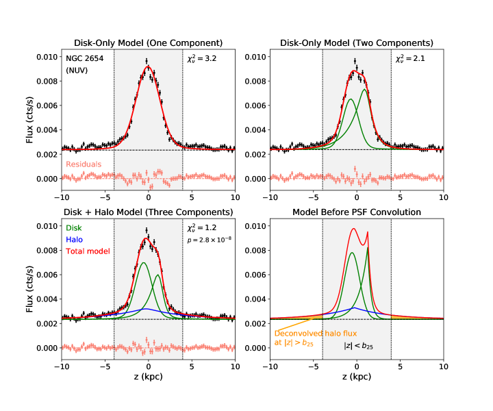
Figure 1: Summary of the procedure used to characterize UV halos, shown here for the example galaxy NGC 2654 in the NUV. We first fit a disk-only model with a single component to the vertical luminosity profile (upper left). We then add a second disk component if this sufficiently improves the quality of the fit ($p\leq 0.05$; upper right). Next, we add the halo component, again if sufficient improvement is seen ($p\leq 0.05$; lower left). We consider the extraplanar luminosity to be the emission in the deconvolved halo at $|z|>b_{25}$ ($\mu_{\text{B}}=25$ mag arcsec${}^{-2}$), as shown at lower right; all emission within $|z|\leq b_{25}$ is considered stellar light.

Secondly, the luminosity profiles of the disks are intrinsically complex. The UV traces young, clumpy stellar populations and is highly susceptible to extinction, resulting in more irregular profiles than in the optical or near infrared. In principle, we expect the disks to be well fit by a single exponential distribution. However, in practice, the UV disks can depart from single exponentials due to structure in the stellar population, including multiple (e.g., thin and thick) disks, clumping of star-forming regions, and disk perturbations such as warps. Additionally, the disk emission is modified by central dust lanes and other anisotropic extinction. The PSF often prevents disentangling which of these effects are at play. This motivates testing disk models of different forms (exponential and Gaussian) and number of components (one or two disk components), as discsused below. There may also be intrinsic differences between the disks in the FUV and the NUV (the former of which traces younger stars), depending on the ages and spatial distributions of the stellar populations. We thus fit the FUV and NUV profiles separately. We use the IDL routine mpfitfun to perform the fit, which employs a Levenberg-Marquardt least-squares minimizer. We report the best-fit values and the errors determined from the diagonal terms of the covariance matrix returned by mpfitfun. In the following sections, we provide details on the model fitting for individual (§ 3.3.1 and § 3.3.2) and stacked galaxies (§ 3.3.3).

3.3.1 Fitting Individual Galaxies - the Disk

The complexities discussed above require us to diversify the disk model set beyond single exponential disks. We select this model set by empirically determining the simplest distributions that well fit the disk profiles. We first consider single exponential and Gaussian profiles; the former nominally describes a smooth disk, while the latter describes a clumpier stellar population. We find that approximately half of the sample galaxies are better fit by a Gaussian profile than by an exponential. We thus allow for use of a Gaussian profile if it provides an improved fit compared to an exponential.

We find that the disks are not well fit by a single component in approximately one third of the galaxies. We therefore allow for a second disk component if it significantly improves the fit using an F-test as described below. We add either an exponential or a Gaussian component, depending on which better improves the fit. We thus arrive at disks modeled by two exponentials (i.e., two smooth disks), an exponential and a Gaussian (a smooth disk modified by clumping), or two Gaussians (a highly clumpy distribution).

We now describe the fitting procedure quantitatively. The exponential disk is of the form:

$$f(z)_{\text{d}}=\begin{cases}f_{0,\text{d}}e^{-\frac{|z|}{h_{\text{d1}}}}&\text{if $z\leq z_{0}$}\\ f_{0,\text{d}}e^{-\frac{|z|}{h_{\text{d2}}}}&\text{if $z>z_{0}$},\end{cases}$$ (1)

where $z$ is the distance from the midplane, $z_{0}$, and $f_{0,\text{d}}$ is the flux at $z_{0}$. The exponential scale heights, $h_{\text{d1}}$ and $h_{\text{d2}}$, are allowed to differ on each side of the disk. This accounts for projection effects in galaxies at lower inclination angles. The Gaussian takes the form:

$$f(z)_{\text{d}}=f_{0,\text{d}}e^{-z^{2}/(2h_{\text{d}}^{2})},$$ (2)

where $h_{\text{d}}$ is the scale height. As the Gaussian distribution is intended to describe clumping rather than a smooth disk, we do not allow the scale height to vary on each side of the disk.

As shown in the top left panel of Fig. 1, we first select either a single exponential or a single Gaussian model based on the fit with the lowest $\chi_{\nu}^{2}=\chi^{2}/\nu=\sum\limits_{i}((f_{i,\text{obs}}-f_{i,\text{mod}})^{2}/\sigma_{i}^{2})/\nu$. Here, $f_{i,\text{obs}}$ and $f_{i,\text{mod}}$ are the observed and modeled fluxes in the $i$th spatial bin, respectively, and $\sigma_{i}$ is the uncertainty on the observed quantity. The number of degrees of freedom, $\nu=N-m$, is the difference between the number of spatial bins, $N$, and the number of free parameters, $m$. All quality-of-fit statistics are computed over $|z|\leq 2b_{\text{25}}$.

Next, as shown in the top right panel of Fig. 1, we assess whether an additional disk component is required using an F-test. We fit two, two-component disk models by adding an exponential or a Gaussian component to the original best-fit model; the parameters of both the first and second components are allowed to vary in the two-component fit. We then calculate an F-statistic of the form:

$$F=((\chi_{1}^{2}-\chi_{2}^{2})/(m_{2}-m_{1}))/\chi_{\nu,2}^{2}.$$ (3)

Here, the subscripts refer to the $\chi^{2}$, $\chi_{\nu}^{2}$, and $m$ values for the one- (1) and two-component models (2). We then compute the F-test probability, $p$; this quantifies the likelihood that improvement in the model fit due to the addition of the second component occurs by chance. If $p\leq 0.05$ for either of the two-component models, we adopt this model as the best fit. In the case that this condition is met for both models, we select the model with the lower $p$ value.

To ensure that the second disk component is physically motivated, we impose several priors on the fit. The second component is intended to characterize structure in the disk rather than emission on halo scales. Thus, we set the prior that the scale heights of both disk components do not exceed the scale height determined from the one-component model (the prior is imposed based on the maximum scale height in the case of the asymmetric exponential profile). We also intend for the weaker component to be sufficiently strong to reflect true sub-structure, and we thus set a prior that the amplitude of the second component is at least $10\%$ of the amplitude of the one-component model. The centroids of both components are allowed to vary from $z_{0}$ above. To robustly detect extraplanar emission, it is more important to appropriately assign the disk emission to the disk component(s) than to recover the intrinsic properties (e.g., scale height) of the disk. We emphasize that the goal is to select the simplest model that well characterizes the disk distribution, so that the presence of extraplanar light can be assessed.

3.3.2 Fitting Individual Galaxies - the Halo

We next test whether a halo component is present (see the bottom left panel of Fig. 1). We consider only an exponential profile for the halo. This is empirically motivated by our sample and by past studies of UV halos, which find that the halo morphologies resemble thick disks (e.g., 2016ApJ...833...58H). The profile has the form:

$$f(z)_{\text{h}}=f_{0,\text{h}}e^{-\frac{|z-z_{0,\text{h}}|}{h_{\text{h}}}}.$$ (4)

Here, $f_{0,\text{h}}$ is the halo flux at $z_{0,\text{h}}$ and $h_{\text{h}}$ is the halo scale height. We impose several priors to ensure that the halo is a sub-dominant component that is more spatially extended than the disk. We do not allow $f_{0,\text{h}}$ to exceed half of the amplitude of the best-fit one-component disk model or $h_{\text{h}}$ to be less than the maximum scale height selected by the best-fit (one- or two-component) disk model. We assume that the midpoint of the halo, $z_{0,\text{h}}$, lies in the midplane of the galaxy. For a one-component disk model, we assume that the disk midpoint reflects the true midplane, and we tie the midpoints of the disk and the halo together ($z_{0,\text{h}}$ = $z_{0}$). For a two-component disk model, neither of the disk midpoints may reflect the true midplane if they capture clumpy sub-structure. We thus require the halo midpoint to fall within 10% of the observed FWHM of the profile peak.

We expect UV halos to have the same scale height in the FUV and NUV. For galaxies with data available in both bands, we can more precisely measure the halo scale heights and luminosities by imposing this restriction than from either band alone. For these galaxies, if a halo is detected in at least one band, we re-perform the fit in the FUV and NUV simultaneously on a grid in halo scale height ($h_{\text{h}}=0.5-8.0$ kpc, in steps of $0.5$ kpc) and fractional NUV flux in the halo ($f_{\text{h,NUV}}=0.05-0.95$, in steps of 0.05). From dust models (e.g., 2001ApJ...548..296W), we expect reflection nebulae to be either bluer than the disks or comparable in color, and we require the fractional flux in the FUV to match or exceed that in the NUV. We adopt the the best-fit disk model as determined for each band in § 3.3.1, but we allow the disk parameters to vary between grid points.

Assuming a likelihood of the form $\mathcal{L}\propto e^{-\chi^{2}/2}$, we construct marginalized probability distribution functions for the halo scale heights and fractional fluxes by calculating a joint $\chi^{2}$ over both bands. From the cumulative distribution functions, we report the median as the best-fit value and the $68$% confidence interval as the $1\sigma$ uncertainties. For both the single-band and two-band fits, we again assess the need for the halo component by calculating the F-statistic (Eq. 3) and corresponding $p$-value. In addition to requiring $p\leq 0.05$ to adopt the halo model, we also require that the best-fit value of $f_{\text{h,NUV}}$ exceed zero at the $\geq 2\sigma$ level. The latter removes cases of weak detections; visual inspection indicates that at least some of these cases are due to non-linear structure in the background. These conservative criteria favor fidelity of the halo detections at the potential expense of the loss of a small number of weak detections.

3.3.3 Fitting Stacked Galaxies

We follow the procedures in § 3.3.1 and § 3.3.2 to fit a simplified set of models to the vertical luminosity profiles of the galaxy stacks. The disks of the stacked profiles are well described by a single Gaussian, with a $\chi^{2}$ test preferring a Gaussian disk to an exponential disk for all stacks. This is a result of the second PSF convolution performed after projecting the profiles to $D_{\text{max}}$ (see § 3.2); due to the double convolution, the vertical profile of the disk approximates the true profiles convolved with the Gaussian core of the PSF at the original (observed) distances. We thus fit a single Gaussian disk model (Eq. 2), refit adding an exponential halo (Eq. 4), and assess the need for the halo component using the F-test (Eq. 3). We apply the same halo priors and detection criteria as for the individual galaxies.

We use bootstrap resampling to determine the probability distributions of the model parameters. For each bin containing $N_{\text{gal}}$ galaxies, we resample the galaxies $10^{3}$ times, drawing $N_{\text{gal}}$ galaxies each time with replacement. We then construct the galaxy stack and perform the fit as described above for each resampled set of galaxies. For each model parameter, we construct the probability distribution from the best-fit values determined from each fit, and we report the median value and the $68$% confidence interval as the corresponding $1\sigma$ uncertainties. The halo detection rates and scale heights are consistent between the bands within the uncertainties, and thus we do not perform the multi-band grid search for the galaxy stacks.

3.3.4 Quantifying Extraplanar Emission

The goal of this analysis is to quantify the UV luminosity of extraplanar emission. This requires defining “extraplanar”. As our objective is to identify scattered light from a dusty disk-halo interface and/or CGM, we seek to separate scattered light as cleanly as possible from starlight. The model profile fitting provides a starting point by separating the light into disk and halo components. However, a significant fraction of the light in the halo component is co-spatial with the disk, and this light may come from the stellar population rather than from a reflection nebula. We therefore define a distance from the disk, $|z|=b_{25}$, which separates planar and extraplanar emission, where $b_{25}$ is defined as in § 2.2. We consider all light in the halo component found at $|z|>b_{\text{25}}$ to be extraplanar emission and all other light to be starlight. We illustrate this distinction in the bottom right panel of Fig. 1. Throughout this work, the term “halo” is used to refer to the model component defined in § 3.3.2, while “extraplanar emission” is used to refer to the light in this component found at $|z|>b_{\text{25}}$.

$b_{25}$ is chosen to conservatively enclose the thin and thick stellar disks within $|z|<b_{25}$. The median value of $b_{25}$ in the sample, $b_{25}\approx 3$ kpc, is a factor of $\gtrsim 6$ and $\sim 3$ times the typical thin- and thick-disk scale heights in an $L^{*}$ galaxy, respectively. In § 4.1, we show that only a few percent of the light in the disk component is typically found at $|z|>b_{\text{25}}$, demonstrating that this is a reasonable demarcation between starlight and extraplanar emission. It is possible that significant scattered light is found within $|z|<b_{25}$, and thus this criterion provides a conservative measure of the extraplanar emission in order to ensure minimal contamination by starlight.

4 Results

4.1 Individual Galaxy Results

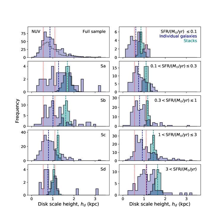
Figure 2: Measured disk scale heights are broadened beyond typical thin disk scale heights due to clumpy UV morphologies, inclined disks ($i<90^{\circ}$), and the GALEX PSF. The NUV disk scale heights for the individual galaxies and the stacks are shown in blue and cyan, respectively; the median is given by the dashed lines. The full sample is displayed at the upper left; the FUV distribution is shown as the dashed histogram for comparison. We separate the sample by morphological type in the remainder of the left column and by SFR in the right column. The stack distributions result from bootstrap resampling and are renormalized for display purposes. The dotted red lines indicate the NUV PSF (FWHM/$2\sqrt{2\ln{2}}$) at $D=50$ Mpc and $D=100$ Mpc. See Appendix LABEL:sec:supp_fuv for the equivalent figure for the FUV data.

We first consider evidence for extraplanar emission from the individual galaxies. We report the disk properties in Tab. LABEL:tab:disks, including the best-fit disk model, flux, fractional flux at $|z|>b_{25}$, scale height(s), and FUV - NUV color. The observed and modeled profiles of three example galaxies are shown in Appendix LABEL:sec:lum_prof. The best-fit model for $37$% of the sample in the NUV ($31$% in the FUV) requires two disk components, demonstrating that clumpiness in the stellar population is relatively common in the sample.

We show the distributions of the disk scale heights for the full sample in the top panel of Fig. 2 (for galaxies with asymmetric profiles and/or multiple components, the median scale height is shown). The scale heights are generally consistent between the FUV and NUV within the errors. The median scale height in the NUV (FUV) is $h_{\text{d}}=0.9$ kpc ($h_{\text{d}}=0.8$ kpc), with $68$% of the sample ranging from $h_{\text{d}}=0.5-1.4$ kpc ($h_{\text{d}}=0.5-1.3$ kpc). The somewhat smaller scale heights in the FUV may reflect the fact that the youngest stars are generally found in the thinnest disks. However, the median value is significantly larger than the stellar thin disk scale heights typically observed in the Milky Way and nearby, resolved galaxies ($h_{\text{d}}\approx 0.2-0.4$ kpc).

Several effects contribute to measuring unphysically large disk scale heights. First, the scale height measurement assumes a perfectly edge-on disk, whereas our sample has a range of inclination angles ($i\gtrsim 75^{\circ}$). The measurement may also be inflated by clumpiness in the stellar population and other morphological perturbations, such as those induced by interactions. Additionally, the projected size of the PSF (FWHM/$2\sqrt{2\ln{2}}$ $\approx 0.5$ kpc at $D=50$ Mpc and $\approx 1.0$ kpc at $D=100$ Mpc in the NUV) makes it difficult to measure the scale height of an unresolved disk even when accounting for PSF convolution in the model profiles.

In Fig. 2, we separate the disk scale heights into bins by morphology and SFR for the NUV (see Appendix LABEL:sec:supp_fuv for the equivalent figure for the FUV). A slight evolution is seen in the scale height with morphological class, with the thinnest disks observed in the latest type galaxies, as expected. Additionally, there is a weak trend toward larger scale heights with increasing SFR; this trend is also expected, as higher SFRs are typically found in more massive disks. However, the PSF causes the measured disk scale heights to be biased high for all morphological types and SFRs, due to the difficulty of resolving disks with scale heights significantly smaller than the PSF.

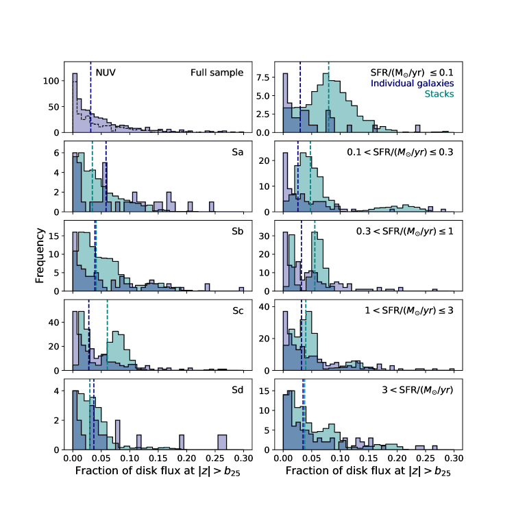
Figure 3: Fractional disk flux at $|z|>b_{\text{25}}$, $f_{\text{d,out}}^{\prime}$, is typically a few percent for the individual galaxies (blue) and the stacks (cyan), demonstrating that $b_{\text{25}}$ reasonably separates planar and extraplanar emission. The stacked distributions are bootstrap resampled. The colors and linestyles are the same as in Fig 2. See Appendix LABEL:sec:supp_fuv for the equivalent figure for the FUV data.

Table 1: Disk properties of the sample galaxies

(1)	(2)	(3)	(4)	(5)	(6)	(7)	(8)	(9)
Galaxy	Disk model	$F_{\text{d}}$	$f_{\text{d},\text{out}}^{\prime}$	$h_{z,1}$	$h_{z,2}$	$h_{z,3}$	$h_{z,4}$	FUV - NUV
		(mJy)		(kpc)	(kpc)	(kpc)	(kpc)	(mag)
NUV
PGC000012	1G	$0.64\pm 0.02$	$0.08$	$2.37\pm 0.06$	-	-	-	$0.45\pm 0.04$
PGC000192	1G	$0.520\pm 0.008$	$0.009$	$1.49\pm 0.03$	-	-	-	-
UGC00043	1G	$0.203\pm 0.007$	$0.05$	$1.13\pm 0.06$	-	-	-	$0.44\pm 0.06$
…	…	…	…	…	…	…	…	…
FUV
PGC000012	GE	$0.40\pm 0.01$	$0.03$	$1.70^{+0.6}_{-1.0}$	-	$0.84^{+1.5}_{-0.7}$	$1.3\pm 0.6$	$0.45\pm 0.04$
PGC000192	-	-	-	-	-	-	-	-
UGC00043	1E	$0.129\pm 0.006$	$0.22$	$1.5\pm 0.2$	$0.8\pm 0.1$	-	-	$0.44\pm 0.06$
…	…	…	…	…	…	…	…	…

Note. — (1) Galaxy name, (2) disk model; 1G = one Gaussian component, 1E = one exponential component, 2G = two Gaussian components, 2E = two exponential components, GE = one Gaussian and one exponential component, (3) total disk flux, (4) fraction of the disk flux at $|z|>b_{\text{25}}$, $f_{\text{d,out}}^{\prime}=F_{\text{d,out}}/F_{\text{d}}$, (5) - (8) disk scale height(s); up to four values are given depending on the number of components (1 or 2) and their symmetry (Gaussian) or asymmetry (exponential), and (9) the FUV - NUV disk color. We correct $F_{\text{d}}$ for Galactic extinction following 2007ApJS..173..293W; this treatment assumes the extinction law of 1989ApJ...345..245C with $R_{\text{V}}=3.1$, yielding $A_{\lambda}/E(B-V)=8.24$ and $8.20$ in the FUV and NUV, respectively. We adopt $E(B-V)$ from 2011ApJ...737..103S. Scale heights without error bars are fixed to the value of the prior defined in § 3.3.1. The full table is available in the online-only materials.

We show the fractional deconvolved flux in the disk at $|z|>b_{\text{25}}$, $f_{\text{d,out}}^{\prime}=F_{\text{d,out}}/F_{\text{d}}$, in Fig. 3 (here the prime notation is used to distinguish this quantity from that which defines the denominator as the total flux, $f_{\text{d,out}}=F_{\text{d,out}}/(F_{\text{d}}+F_{\text{h}})$). The distributions are similar in both bands and are strongly peaked toward minimal disk flux outside of $b_{\text{25}}$. In the NUV (FUV), we find a median $f_{\text{d,out}}^{\prime}=0.03$ ($f_{\text{d,out}}^{\prime}=0.02$). Additionally, this is a minority of the total deconvolved flux at $|z|>b_{\text{25}}$ in galaxies with halos. Thus, in general, the use of $b_{25}$ to separate the planar and extraplanar emission is reasonable. At the same time, $35$% of galaxies have $f_{\text{d,out}}^{\prime}\geq 0.05$ in the NUV; this number is $32$% in the FUV.

The light in the extended disk may come from several sources. 2018ApJ...862...25J fit the GALEX FUV and NUV profiles of 38 nearby, edge-on disk galaxies with single exponential profiles, finding a modest median scale height of $h\approx 0.5$ kpc, consistent with a thick disk. They demonstrate a strong positive correlation between the UV and H$\alpha$ scale heights, suggesting that the extended UV emission comes from scattered light in the thick disk of the dusty ISM. However, it is also possible that the H$\alpha$-emitting gas is at least partially ionized by a thick stellar disk of hot, low-mass evolved stars (2011MNRAS.415.2182F), which may be responsible for producing some of the UV emission. Additionally, due to the large sample size, we adopt a simple definition of the region considered to be extraplanar, and there are instances in which perturbations to the structure of the stellar disk (e.g., warps) produce emission in this region. The disk wings at $|z|>b_{\text{25}}$ are likely a combination of starlight and scattered light from a dusty disk-halo interface. We therefore consider the disk light at $|z|>b_{\text{25}}$ to be an upper limit on additional extraplanar emission, above that measured from the halo light at $|z|>b_{\text{25}}$.

Table 2: Halo properties of the sample galaxies

(1)	(2)	(3)	(4)	(5)	(6)	(7)
Galaxy	$F_{\text{h}}$, NUV	$F_{\text{h}}$, FUV	$f_{\text{h,out}}$, NUV	$f_{\text{h,out}}$, FUV	$h_{\text{h}}$	FUV - NUV ($|z|>b_{\text{25}}$)
	(mJy)	(mJy)			(kpc)	(mag)
NGC0085B	$0.04^{+0.02}_{-0.01}$	$0.018^{+0.009}_{-0.005}$	$0.06$	$0.07$	$4.2^{+2.6}_{-2.0}$	$0.65^{+0.06}_{-0.10}$
IC0045	$0.09^{+0.04}_{-0.03}$	-	$0.17$	-	$5.8^{+1.6}_{-2.3}$	-
PGC087843	$0.06\pm 0.02$	-	$0.25$	-	$5.5^{+1.8}_{-2.5}$	-
…	…	…	…	…	…	…

Note. — (1) Galaxy name, (2) total halo flux (NUV), (3) total halo flux (FUV), (4) fractional flux in the halo at $|z|>b_{\text{25}}$, $f_{\text{h,out}}=F_{\text{h,out}}/(F_{\text{d}}+F_{\text{h}})$ (NUV), (5) fractional flux in the halo at $|z|>b_{\text{25}}$ (FUV), (6) halo scale height, (7) FUV - NUV halo color at $|z|>b_{\text{25}}$. The halo flux is corrected for Galactic extinction as described in Tab. LABEL:tab:disks. The full table is available in the online-only materials.