Spin-Dependent Force and Inverted Harmonic Potential for Rapid Creation of Macroscopic Quantum Superpositions
Abstract
Creating macroscopic spatial superposition states is crucial for investigating matter-wave interferometry and advancing quantum sensor technology. Currently, two potential methods exist to achieve this objective. The first involves using inverted harmonic potential (IHP) to spatially delocalize quantum states through coherent inflation [1]. The second method employs a spin-dependent force to separate two massive wave packets spatially [2]. The disadvantage of the former method is the slow initial coherent inflation, while the latter is hindered by the diamagnetism of spin-embedded nanocrystals, which suppresses spatial separation. In this study, we integrate two methods: first, we use the spin-dependent force to generate initial spatial separation, and second, we use IHP to achieve coherent inflating trajectories of the wavepackets. This approach enables the attainment of massive large spatial superposition in minimal time. For instance, a spatial superposition with a mass of kg and a size of 50 m is realized in seconds. We also calculate the evolution of wave packets in both harmonic potential (HP) and IHP using path integral approach.
I Introduction
The significant interest in massive quantum superposition states primarily arises from three aspects. The first is the exploration of the quantum-classical boundary [3]. Quantum interference, from electrons to macromolecules ( kg), has been observed in contemporary experiments, demonstrating their quantum nature [4, 5, 6, 7, 8]. This leads to quests about whether quantum superposition states can also be achieved for objects of larger mass [9]. The second aspect is their utility in validating theoretical models [10]. For instance, they can be employed to test wave function collapse theories [11, 12], modified quantum mechanical frameworks [13, 14, 15], and examine the weak equivalence principle [16, 17]. Additionally, they may reveal the quantum nature of gravity by combining two massive spatial superposition states [18, 19, 20, 21], see theoretical explanations [22, 23, 24, 25, 26, 27, 28].
The third aspect is that they can act as highly sensitive quantum sensors, detecting phenomena such as the Casimir force and dipole interactions [29, 30, 31, 32], gravitational waves [33, 34], quantum sensors for detecting accelerations, and inertial rotations [35, 36, 37], dark matter [38], physics beyond the Standard Model [39], testing massive graviton [40], non-local gravitational interaction [22, 41], and analogue of light bending experiment in quantum gravity [42].
Advancements in quantum technology have enabled the fabrication of massive quantum superposition states. A critical challenge in realizing these states is decoherence, induced by gas molecule scattering and the emission and absorption of thermal photons, dipoles and electromagnetic interactions [43, 15, 44, 45]. However, this decoherence effect can be effectively minimized through levitation mechanics in ultrahigh vacuum environments [46]. It is now feasible to simultaneously cool the internal degrees of freedom (phonons) and the mechanical degrees of freedom (center-of-mass (CoM) motion) of nano-objects ranging from to kg to a quantum ground state [47, 48, 49]. Additionally, atom chips are employed to control magnetic fields precisely [50]. Recently, a full-loop Stern-Gerlach interferometer for \ce^87Rb atoms was realized for the first time using magnetic fields generated by atom chips [51]. Furthermore, embedding a single nitrogen-vacancy (NV) centre in nanodiamonds has achieved electron spin coherence times of ms [52, 53].
Based on these cutting-edge techniques, numerous experimental schemes for creating macroscopic spatial superposition states have been proposed [15, 2, 54, 55, 1, 56, 57, 58, 59, 60, 32]. A natural method to achieve a delocalized quantum state is to allow a quantum wave packet to evolve freely [15]. However, this delocalization process is slow. For instance, consider a silica microsphere with a mass of kg trapped by a magnetic field at a frequency of 100 Hz and cooled to its ground state [61]. Its initial wave packet spatial width is approximately m. After 1 s of free evolution, the wave packet width becomes about m, roughly one-thousandth of its size. To accelerate this delocalization process, an IHP can induce coherent inflation [1, 62]. This approach allows the coherent length of a kg nanoparticle to increase to around 1 m in 0.6 s, making the coherence length comparable to its size. Another method for creating macroscopic spatial superposition states involves utilizing spin-dependent forces, such as using diamond embedded with a NV center [2, 54, 57, 56]. Initially, a pulse is used to place the electron spin of the NV center in a superposition state, followed by applying a magnetic field to induce spatial splitting, similar to the Stern-Gerlach experiment. The advantage of this method is the ease of preparing the initial superposition state and reading out the final spin state [63]. However, the diamagnetism of the diamond suppresses the spatial separation of the wave packets when an external magnetic field is applied [59, 64, 65, 66], limiting the direct increase of the superposition size through enhanced magnetic field gradients.
In this work, we combine spin-dependent forces and IHP to achieve a massive large spatial superposition in a relatively short time. Initially, the spin-dependent force is used to create a spatial separation between two massive wave packets. Subsequently, the IHP facilitates rapid separation of the wave packets. This approach addresses the challenges of slow acceleration in the early stages of the IHP [1, 62] and the suppression of superposition size due to diamagnetism [56, 57, 32, 59, 64, 67, 65, 66].
The paper is organized as follows. Section II presents the specific experimental protocol and the magnetic fields required to construct the HP and IHP for the experiment. Section III provides an analytical solution for the classical trajectories of the wave packets at each experiment stage. In Section IV, we numerically calculate the classical trajectories of the wave packet without approximations for the nonlinear magnetic field and compare these results with the analytical solution. Section V discusses the evolution of the wave packet under HP and IHP using path integrals. In Section VI, we examine the effect of fluctuations in the magnetic field gradient on wave packet contrast for both the HP and IHP cases. Finally, we conclude our findings in Section VII.
II Experimental scheme
The Hamiltonian of the nanodiamond embedded with a NV center in the presence of an external magnetic field is given by:
| (1) |
The first term represents the kinetic energy of the nanodiamond, where is the momentum and is the mass of the nanodiamond. The second term signifies the magnetic energy of a diamagnetic material (nanodiamond) in a magnetic field, with as the mass susceptibility and as the vacuum permeability. The third term is electron spin interacting with the magnetic field. is the reduced Plank constant and the electronic gyromagnetic ratio. is the spin operator. is the magnetic field. The last term represents the zero-field splitting of the NV center with GHz. is the spin component operator aligned with the NV axis. In this paper, we will assume that the nanodiamond’s rotational angular momentum is zero; see for a finite angular momentum and its implications [64]
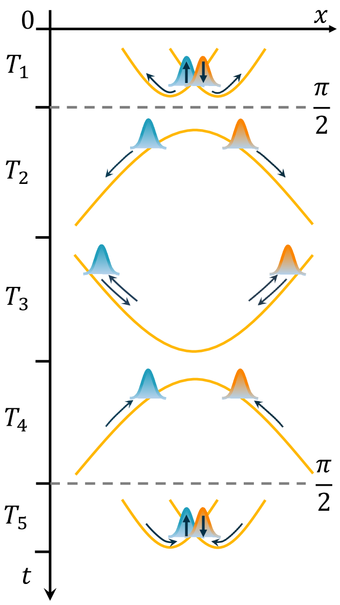
The experimental protocol is divided into five stages: the initial separation stage, the enhancement stage, the return stage, the deceleration stage, and the recombination stage. This division aims to achieve a large spatial superposition size in a short time (around 0.1 s) and to recombine the trajectories of the CoM, thereby restoring spin coherence [51]. The five stages are outlined in Fig. 1 and described below.
-
•
Initial state: The initial state is a spin superposition state , and and are eigenstates with eigenvalues of 1 and -1 for the spin operator .
-
•
Initial separation stage (Stage 1): Switching on an external linear magnetic field, the wave packets with different spin eigenstates generate spatial separation in the HP.
-
•
Enhancement stage (Stage 2): When the spatial separation of the two wave packets in the HP is maximized, the linear magnetic field is switched off. Then a pulse is applied to transform the state into [68, 69]. We ignore the time of applying the pulse here. Subsequently, switching on the nonlinear magnetic field creates an IHP allowing the wave packets to separate rapidly, increasing the superposition size in a short period of time.
-
•
Return stage (Stage 3): The nonlinear magnetic field is switched off, and the linear field is switched on after the wave packet has evolved in the IHP for a while 111The exact evolution time is related to the superposition size we want to achieve. The longer the time, the larger the spatial separation between the wave packets.. The velocities of the wave packets gradually decrease in the HP and then reverse. The spatial separation between wave packets reaches its maximum at this stage.
-
•
Deceleration stage (Stage 4): When the magnitude of the wave packet velocity is the same as the magnitude at the end of the second stage and in the opposite direction, the linear magnetic field is switched off and the nonlinear magnetic field is switched on. The wave packet gradually decelerates in the IHP.
-
•
Recombination stage (Stage 5): The nonlinear magnetic field is switched off when the wave packet velocity decreases to zero. A pulse is then applied to transform the state from to . The linear magnetic field is then switched on. The gradient of the magnetic field is fine-tuned so that the trajectories of the two wave packets are closed after half a period.
For clarity, we use terms like ”initial separation stage” and ”Stage 1” interchangeably without ambiguity in the following sections. To simplify the discussion, only the magnetic field component in the x-direction is considered to construct the one-dimensional HP and IHP. The HP can be obtained using a linear magnetic field [2, 56]:
| (2) |
where is a bias field along the x-direction and is the gradient corresponding to the linear magnetic field. Substituting Eq.(2) into the Hamiltonian Eq.(1) one have:
| (3) |
The superscript “H” denotes the HP. is the frequency of the HP. The IHP can be obtained by means of a nonlinear magnetic field [59]:
| (4) |
where is the gradient parameter corresponding to the nonlinear magnetic field. Note that the dimension of is . Substituting Eq.(4) into the Hamiltonian Eq.(1) one have:
| (5) |
Here term has been ignored. This is because this term is zero during the enhancement and deceleration stages. It follows from Eq.(1) that the IHP is obtained when the condition is satisfied 222When this condition is not satisfied, we get a quartic potential. This potential can also be used to create macroscopic spatial superposition [70]. The evolution of the wave packet in the quartic potential can be solved analytically and numerically [71, 72].. At this point, the Hamiltonian can be written as:
| (6) |
The superscript “I” denotes the IHP. is the frequency of the IHP.
III CoM trajectory and superposition size
The expectation value of position operator satisfies the equation of motion:
| (7) |
Since the trajectories of the two wave packets are completely symmetric, to simplify the calculation process, we take the wave packet with the spin quantum number as an example to calculate the classical trajectory. For convenience of representation, we make the conventions shown in Table 1.
| Symbol | Meaning |
| The frequency of the harmonic or inverted harmonic potential at the i-th stage. | |
| The classical trajectory of the i-th stage. | |
| The classical position at the end of the i-th stage. | |
| The classical velocity at the end of the i-th stage. | |
| The time variable at the i-th stage. | |
| The time interval at the i-th stage.333For example, at the beginning of the i-th stage and at the end of that stage . |
Stage 1 — Substituting the Hamiltonian Eq.(II) into Eq.(7) and then taking the second order derivative of the expectation value of the position operator with respect to time gives:
| (8) |
where is the frequency of the HP in the initial separation stage. The term in Eq.(8) does not affect the maximum superposition size in the initial separation stage. To be consistent with the coordinates of the later stages, we set in the initial separation stage equal to zero. Considering the initial conditions and , the solution of Eq.(8) is:
| (9) |
When , the superposition size achieves the maximum value in the initial separation stage. The position of the CoM at this point is taken as the initial condition to solve the equation of motion for the enhancement stage.
Stage 2 — Using Eq.(7) again and considering the Hamiltonian in Eq.(6), one can obtain the CoM trajectory for the enhancement stage:
| (10) |
where
| (11) |
The is the frequency of the IHP in the enhancement stage.
Stage 3 — At the end of the enhancement stage, the position and velocity of the CoM are:
| (12) |
Taking the position and velocity of the CoM as the initial conditions and then combining Eq.(II) and (7) yields the trajectory of the CoM in the return stage:
| (13) |
where
| (14) |
The is the frequency of the HP in the return stage. The superposition size reaches its maximum value when . The maximum superposition size is:
| (15) |
where
| (16) |
is a dimensionless quantity. The maximum superposition size can be rewritten as:
| (17) |
The time corresponding to the maximum superposition size at the stage 3 is:
| (18) |
We set the time interval of stage 3 to be . This is not necessary, but doing so makes the enhancement and deceleration stages symmetric. This is because, at the end of stage 3, the wave packet returns to its initial position, at which point its velocity is equal in magnitude and opposite in direction to the velocity at the beginning of the stage. We can use the same IHP as in the enhancement stage to decelerate the wave packet, thereby finally closing the wave packet trajectories. At the end of stage 3, the position and velocity of the CoM are:
| (19) |
Stage 4 — Using the position and velocity at the end of the return stage as the initial conditions for the deceleration stage, similar to the enhancement stage, the CoM trajectory for the deceleration stage can be found by using Eq.(6) and (7) as:
| (20) |
where is the frequency of the IHP in the deceleration stage. Deriving Eq.(20) with respect to time and making it equal to zero gives the time
| (21) |
required for the CoM velocity to decrease to zero. Substituting the evolution time into Eq.(20) gives the position of the CoM at this time
| (22) |
If is assumed, then one have . The reason for the negative sign is that the position is opposite in sign to the velocity at the end of return stage and should be greater than zero. However, Substituting this into gives . This is because as the CoM gets closer to the origin position, the velocity gets smaller, and at the same time the acceleration also gets smaller and eventually tends to zero. Therefore the time for the CoM to decelerate to zero tends to infinity. To avoid this situation, can only take a small value other than zero. This is why the recombination stage is needed to close the CoM trajectory.
Stage 5 — The equation of motion for the final stage (recombination stage) is the same as the initial separation stage but with a different frequency. The solution is:
| (23) |
where is the frequency of the HP in the recombination stage. The second equation in Eq.(III) holds because the CoM is required to return to the origin after half a period of motion. At this point, the position and momentum of the CoM coincide.
IV Comparing analytic and numerical results
In the analytic calculation of the classical trajectories of the wave packet in Sec.III, we used approximate Hamiltonian (see Eq.(6)) in the second and fourth stages in the presence of a nonlinear magnetic field. In the numerical calculations of this section, we use the Hamiltonian without approximation (see Eq.(II)).
| (T) | (T/m) | (T/) | (s) | |
| 1 | 0 | 2507 | — | 0.01784 |
| 2 | 10 | — | 0.03000 | |
| 3 | 0 | — | 0.00415 | |
| 4 | 10 | — | 0.03000 | |
| 5 | 0 | — | 0.01853 |
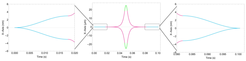
The numerical calculation results are shown in Fig.2. The first stage is the initial separation stage. The time of this stage is (half a period), which is about 0.018 s. Due to their different spin states, the two wave packets move in two different HPs and yield a spatial separation of about 6 nm. The second stage is the enhancement stage. The longer the duration of this stage, the larger the superposition size obtained. However, in order to keep the total running time around 0.1 s, we set the evolution time of this stage to be 0.03 s. With the parameters in Table.2, the spatial separation between the two wave packets at the end of the enhancement stage is about 37.14 m. The third stage is the return stage. In this stage, the two wave packets move away from each other in the HP, and the speed of the wave packets decreases gradually. When the velocity decreases to 0, the spatial separation between them reaches a maximum value of about 50 m. Then, the velocities of the two wave packets are reversed, and they gradually come closer together. We bring the wave packets back to roughly the initial position of this stage by fine-tuning the evolution time 444The fine-tuning of the time is done here to make the trajectory more symmetric, but this tuning is not mandatory. We can also set different evolution times in this stage and then close the trajectory by adjusting the parameters of the later stages and keeping the total evolution time around 0.1 s. to 0.00415 s. The fourth stage is the deceleration stage. As analyzed in stage 4 of Sec.III, this deceleration process takes an infinite time if we want the velocity to decrease to 0 when the trajectories close. So, we make the velocity decrease to 0 when the spatial separation between the wave packets is about 6 nm by fine-tuning the magnetic field gradient. The parameter values used in this stage are shown in Table.2 and the evolution time is 0.03 s 555Here, we set the evolution time to 0.03 s to be symmetric with the second stage. We can also fix the magnetic field gradient and then fine-tune the time to make the velocity of the wave packets decrease to 0 when they are separated by about 6 nm.. The fifth stage is the recombination stage. This stage is the inverse process of the initial separation stage. By fine-tuning the magnetic field gradient and evolution time in this stage, with parameters taking the values shown in Table.2, the wave packets are able to return to the initial position and with a velocity of zero.
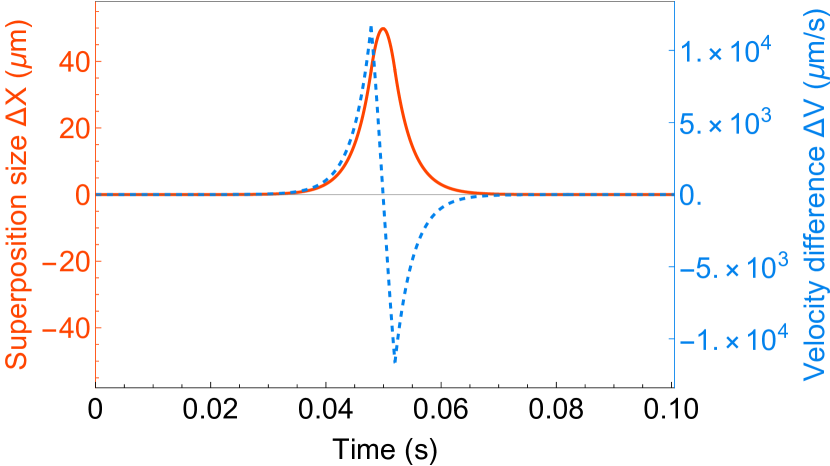
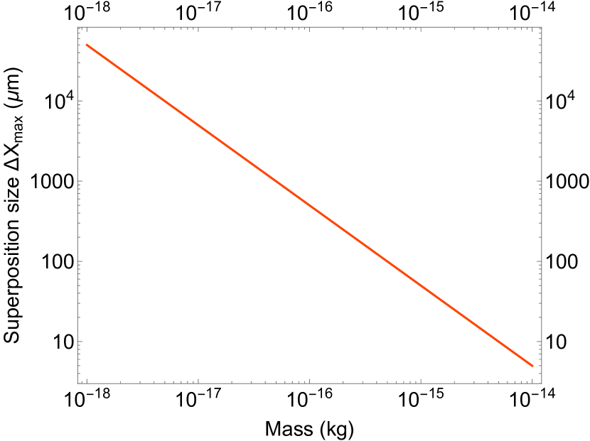
Combining these five stages, the variations in superposition size and velocity differences are shown in Fig.3. The superposition size increases and then decreases, reaching a maximum value of 49.8294 m at t = 0.0499 s. At this point, the velocity difference is , and the velocity of the wave packet starts to reverse. For comparison with the analytical expression, we substitute the parameter values from Table.2 into Eq.(15), which gives a maximum superposition state size of 49.8298 m. The per cent error between the theoretical and numerical calculations is less than %. This indicates that the IHP approximation we made is reasonable. By fixing the magnetic field gradient and evolution time from the first to the third stage to the values shown in Table.2, and then varying the mass, we obtain the scalar behaviour of the superposition size with respect to the mass, as shown in Fig.4.
V Wave packet evolution
If the initial state is a Gaussian shape wave packet666The difference between Gaussian wave packet and Gaussian shape wave packet is that Gaussian wave packet maintains minimum uncertainty but Gaussian shape wave packets do not necessarily maintain this property [73]. (GSWP), then the evolution of the wave packet under HP and IHP can be solved analytically [74, 75, 76, 73]. In Appendix A, we give a detailed procedure for calculating the wave packet evolution using the path integral. In this section, we provide the main results. The general form of a GSWP can be written as:
| (24) |
where is the normalization factor, is the wave packet width, is the center position of the wave packet, and , and are the phase related factors. The factor 1/4 in front of the parameter is set for the convenience of later calculations. A GSWP remains a GWSP after it has evolved in HP and IHP. Their general solutions can be written as:
| (25) |
Where is the spatial width of the wave packet evolving in time and is the classical equation of motion of the wave packet. For the HP case, we have:
| (26) | ||||
| (27) |
where
| (28) |
The index “H” indicates the expression of the physical quantity in the case of HP. For the IHP case, we have:
| (29) | ||||
| (30) |
where
| (31) |
The index “I” indicates the expression of the physical quantity in the case of IHP. The expressions for the other parameters in Eq.(25) for the HP and IHP cases are given in Appendix A. The form of the solution of the wave packet in the IHP are the same as in the HP case, but with the replacement of with and with . If the initial state is a Gaussian wave packet, the values of the parameters in Eq.(24) are:
| (32) |
where is the initial momentum. Substituting these parameters into Eqs.(26) - (31) gives:
| (33) | ||||
| (34) |
and
| (35) | ||||
| (36) |
The Eqs.(33) and (35) for the evolution of the spatial width of the wave packet in HP and IHP are the same as those in [73]. Eqs.(34) and (36) are the same as the classical equations of motion (III) and (20).
VI Fluctuation in magnetic field and wave packet contrast
In this section, we study the effect of fluctuation of the magnetic field on the contrast of the wave packets. Fluctuations in the magnetic field cause deviations from the classical position and momentum of the wave packet, preventing the two wave packets from overlapping and causing a decrease in the contrast of the wave packets. This is also known as the Humpty-Dumpty problem in the Stern-Gerlach interferometer [77].
We mark the wave packets on the two arms of the interferometer as and . The contrast of the wave packets can be defined as:
| (37) |
Since we are considering the effect of classical position and momentum deviations on the contrast, the values of the parameters are the same in and except for (classical position) and (associated with classical momentum). The integral of Eq.(37) can be written as:
| (38) |
where
| (39) |
The and are the classical positions of the wave packets of the left and right arms of the interferometer. The and correspond to the values of the parameter in the left and right wave packets. For Eq.(38), only the exponential decay terms associated with the classical position and momentum deviations are retained while the amplitude and phase factor is neglected [78]. Since both the classical trajectory and the parameter are functions of the gradient 777For a linear magnetic field, is taken as . For a nonlinear magnetic field, is taken as . and time , when there is a small fluctuation in the gradient, Eq.(VI) can be written as:
| (40) |
Note that the change in the parameter is caused by a change in the classical momentum, so the parameter needs to be written as an expression with respect to the momentum . Substituting the expressions for and into Equation (VI) for the HP and IHP cases, and then combining the results with Equation (38), would reveal the effect of fluctuations in the gradient on the contrast in both cases.
VI.1 Wave packet contrast in the case of HP
The expression for the classical momentum in the HP case can be obtained by deriving Eq.(34) with respect to time:
| (41) |
Considering the Gaussian wave packet as an initial condition (see Eq.(32)) and setting the initial momentum , in combination with Eq.(41), the parameter (see Eq.(A.1) in the Appendix A) can be written as:
| (42) |
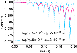
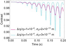
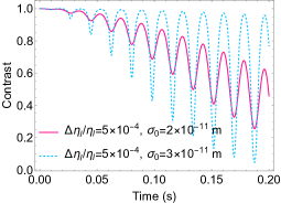
Combining Eq.(34), (38), (VI), (41) and (42) gives the variation of wave packet contrast with time when there is a small fluctuation in the linear magnetic field gradient, as shown in Fig.5. The evolution time is set to 0.2 s to see the changing trend of the contrast more clearly. Over a short period of time, the contrast is generally oscillating and decaying with time. The larger the gradient fluctuation, the faster the decay. The initial wave packet spatial width also has an effect on the contrast. The wider the initial spatial width, the slower the contrast decays.
VI.2 Wave packet contrast in the case of IHP
Derivation of Eq.(36) with respect to time yields the momentum for the IHP case:
| (43) |
Consider also the Gaussian wave packet as an initial condition (see Eq.(32)) and set the initial momentum . Combined with Eq.(43), the parameter (see Eq.(A.2) in the Appendix A) can be written as:
| (44) |
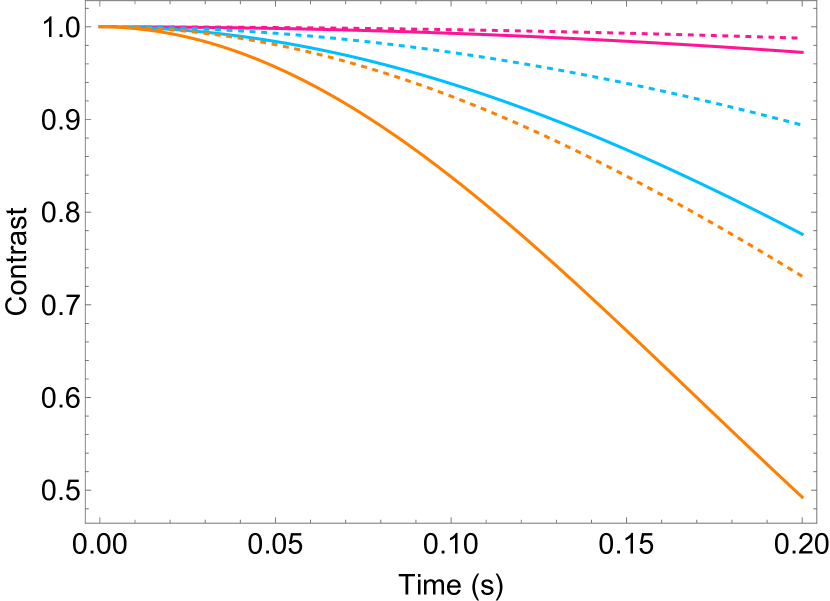
Combining Eq.(36), (38), (VI), (43) and (44) gives the variation of wave packet contrast with time when there is a small fluctuation in the nonlinear magnetic field gradient, as shown in Fig.6. The wave packet contrast decays with time. The smaller the fluctuation , the slower the decay. Also, increasing the initial wave packet spatial width can slow down the wave packet contrast decay.
For both HP and IHP cases, reducing the fluctuation of the magnetic field gradient and increasing the initial wave packet width can suppress the decay of contrast.
VII Conclusion
In this paper, we investigated the use of spin-dependent force and IHP to generate massive large spatial superposition states and construct a full-loop interferometer. The spin-dependent force enables a massive wave packet to achieve a small spatial separation in a short time. Subsequently, the IHP allows this separation to increase rapidly. For a nanodiamond with a mass of kg, we found that a superposition size of 50 m can be achieved in 0.1 s. We also analytically calculated the evolution of the wave packet in both the HP and IHP using path integrals. Additionally, we discussed how fluctuations in the magnetic field gradient affect the wave packet contrast, concluding that smaller gradient fluctuations and a wider wave packet width result in a slower decrease in contrast.
Our study focused on a nanodiamond embedded with an NV centre. The nanodiamond possesses mechanical degrees of freedom (CoM motion), internal degrees of freedom (phonons), and rotational degrees of freedom. Currently, both center-of-mass motion and phonons can be cooled to the ground state [49], and phonons are difficult to excite during movement in HP and IHP [79, 80]. The rotational degree of freedom can affect the final wave packet contrast of the interferometer; however, if the NV center is at or near the nanodiamond center, this effect can be mitigated by fine-tuning the magnetic field and timing [81, 82, 64]. Furthermore, the electron spin coherence time of the NV center can be as long as 1 s at low temperatures and under pure nanocrystal conditions [83, 84, 85]. These findings indicate the feasibility of realizing macroscopic quantum states with masses ranging from to kg and superposition sizes on the order of micrometres in the laboratory.
Note added: Following the completion of our work, we identified corresponding independent research by Sougato Bose’s group (on arXiv today).
acknowledgments
We are grateful to Tian Zhou, Ryan Marshman and Sougato Bose for stimulating discussions. R. Z. and Q. X. are supported by China Scholarship Council (CSC) fellowship. A. M. is supported by Sloan and the Gordon and Betty Moore foundations.
References
- [1] Oriol Romero-Isart. Coherent inflation for large quantum superpositions of levitated microspheres. New Journal of Physics, 19(12):123029, December 2017.
- [2] Matteo Scala, M. S. Kim, G. W. Morley, P. F. Barker, and S. Bose. Matter-wave interferometry of a levitated thermal nano-oscillator induced and probed by a spin. Physical Review Letters, 111(18):180403, 2013.
- [3] Markus Arndt and Klaus Hornberger. Testing the limits of quantum mechanical superpositions. Nature Physics, 10(4):271, 2014.
- [4] A. Tonomura, J. Endo, T. Matsuda, T. Kawasaki, and H. Ezawa. Demonstration of single-electron buildup of an interference pattern. American Journal of Physics, 57(2):117–120, February 1989.
- [5] T. Kovachy, P. Asenbaum, C. Overstreet, C. A. Donnelly, S. M. Dickerson, A. Sugarbaker, J. M. Hogan, and M. A. Kasevich. Quantum superposition at the half-metre scale. Nature, 528(7583):530–533, December 2015.
- [6] Markus Arndt, Olaf Nairz, Julian Vos-Andreae, Claudia Keller, Gerbrand van der Zouw, and Anton Zeilinger. Wave-particle duality of C60 molecules. Nature, 401(6754):680–682, 1999.
- [7] Stefan Gerlich, Sandra Eibenberger, Mathias Tomandl, Stefan Nimmrichter, Klaus Hornberger, Paul J Fagan, Jens Tüxen, Marcel Mayor, and Markus Arndt. Quantum interference of large organic molecules. Nature communications, 2(1):1–5, 2011.
- [8] Yaakov Y. Fein, Philipp Geyer, Patrick Zwick, Filip Kiałka, Sebastian Pedalino, Marcel Mayor, Stefan Gerlich, and Markus Arndt. Quantum superposition of molecules beyond 25 kDa. Nature Physics, 15(12):1242–1245, December 2019.
- [9] Filip Kiałka, Yaakov Y. Fein, Sebastian Pedalino, Stefan Gerlich, and Markus Arndt. A roadmap for universal high-mass matter-wave interferometry. AVS Quantum Science, 4(2):020502, April 2022.
- [10] Sougato Bose, Ivette Fuentes, Andrew A. Geraci, Saba Mehsar Khan, Sofia Qvarfort, Markus Rademacher, Muddassar Rashid, Marko Toroš, Hendrik Ulbricht, and Clara C. Wanjura. Massive quantum systems as interfaces of quantum mechanics and gravity. November 2023.
- [11] Angelo Bassi, Kinjalk Lochan, Seema Satin, Tejinder P Singh, and Hendrik Ulbricht. Models of wave-function collapse, underlying theories, and experimental tests. Reviews of Modern Physics, 85(2):471, 2013.
- [12] Angelo Bassi, Mauro Dorato, and Hendrik Ulbricht. Collapse Models: A Theoretical, Experimental and Philosophical Review. Entropy, 25(4):645, April 2023.
- [13] Stephen L. Adler and Angelo Bassi. Is Quantum Theory Exact? Science, 325(5938):275–276, July 2009.
- [14] Angelo Bassi and GianCarlo Ghirardi. Dynamical reduction models. Physics Reports, 379(5):257, 2003.
- [15] Oriol Romero-Isart. Quantum superposition of massive objects and collapse models. Phys. Rev. A, 84:052121, Nov 2011.
- [16] Sougato Bose, Anupam Mazumdar, Martine Schut, and Marko Toroš. Entanglement witness for the weak equivalence principle. Entropy, 25(3):448, March 2023.
- [17] Sumanta Chakraborty, Anupam Mazumdar, and Ritapriya Pradhan. Distinguishing Jordan and Einstein frames in gravity through entanglement. Phys. Rev. D, 108(12):L121505, 2023.
- [18] Sougato Bose, Anupam Mazumdar, Gavin W Morley, Hendrik Ulbricht, Marko Toroš, Mauro Paternostro, Andrew A Geraci, Peter F Barker, MS Kim, and Gerard Milburn. Spin entanglement witness for quantum gravity. Physical Review letters, 119(24):240401, 2017.
- [19] Sougato Bose. https://www.youtube.com/watch?v=0Fv-0k13s_k, 2016. Accessed 1/11/22.
- [20] Chiara Marletto and Vlatko Vedral. Gravitationally induced entanglement between two massive particles is sufficient evidence of quantum effects in gravity. Physical Review Letters, 119(24):240402, 2017.
- [21] Farhan Hanif, Debarshi Das, Jonathan Halliwell, Dipankar Home, Anupam Mazumdar, Hendrik Ulbricht, and Sougato Bose. Testing whether gravity acts as a quantum entity when measured. 7 2023.
- [22] Ryan J. Marshman, Anupam Mazumdar, and Sougato Bose. Locality and entanglement in table-top testing of the quantum nature of linearized gravity. Phys. Rev. A, 101(5):052110, 2020.
- [23] Daine L Danielson, Gautam Satishchandran, and Robert M Wald. Gravitationally mediated entanglement: Newtonian field versus gravitons. Physical Review D, 105(8):086001, 2022.
- [24] Sougato Bose, Anupam Mazumdar, Martine Schut, and Marko Toroš. Mechanism for the quantum natured gravitons to entangle masses. Phys. Rev. D, 105(10):106028, 2022.
- [25] Daniel Carney. Newton, entanglement, and the graviton. Phys. Rev. D, 105(2):024029, 2022.
- [26] Marios Christodoulou and Carlo Rovelli. On the possibility of laboratory evidence for quantum superposition of geometries. Physics Letters B, 792:64–68, 2019.
- [27] Daniel Carney, Philip C E Stamp, and Jacob M Taylor. Tabletop experiments for quantum gravity: a user’s manual. Classical and Quantum Gravity, 36(3):034001, jan 2019.
- [28] Marios Christodoulou, Andrea Di Biagio, Markus Aspelmeyer, Časlav Brukner, Carlo Rovelli, and Richard Howl. Locally mediated entanglement through gravity from first principles. arXiv preprint arXiv:2202.03368, 2022.
- [29] Thomas W. van de Kamp, Ryan J. Marshman, Sougato Bose, and Anupam Mazumdar. Quantum Gravity Witness via Entanglement of Masses: Casimir Screening. Phys. Rev. A, 102(6):062807, 2020.
- [30] Martine Schut, Alexey Grinin, Andrew Dana, Sougato Bose, Andrew Geraci, and Anupam Mazumdar. Relaxation of experimental parameters in a quantum-gravity-induced entanglement of masses protocol using electromagnetic screening. Phys. Rev. Res., 5(4):043170, 2023.
- [31] Martine Schut, Andrew Geraci, Sougato Bose, and Anupam Mazumdar. Micrometer-size spatial superpositions for the QGEM protocol via screening and trapping. Phys. Rev. Res., 6(1):013199, 2024.
- [32] Ryan J. Marshman, Sougato Bose, Andrew Geraci, and Anupam Mazumdar. Entanglement of magnetically levitated massive schrödinger cat states by induced dipole interaction. Physical Review A, 109(3):L030401, March 2024.
- [33] Asimina Arvanitaki and Andrew A. Geraci. Detecting High-Frequency Gravitational Waves with Optically Levitated Sensors. Physical Review Letters, 110(7):071105, February 2013.
- [34] Ryan J. Marshman, Anupam Mazumdar, Gavin W. Morley, Peter F. Barker, Steven Hoekstra, and Sougato Bose. Mesoscopic Interference for Metric and Curvature (MIMAC) Gravitational Wave Detection. New J. Phys., 22(8):083012, 2020.
- [35] Marko Toroš, Thomas W. Van De Kamp, Ryan J. Marshman, M. S. Kim, Anupam Mazumdar, and Sougato Bose. Relative acceleration noise mitigation for nanocrystal matter-wave interferometry: Applications to entangling masses via quantum gravity. Phys. Rev. Res., 3(2):023178, 2021.
- [36] Meng-Zhi Wu, Marko Toroš, Sougato Bose, and Anupam Mazumdar. Quantum gravitational sensor for space debris. Phys. Rev. D, 107(10):104053, 2023.
- [37] Meng-Zhi Wu, Marko Toroš, Sougato Bose, and Anupam Mazumdar. Inertial Torsion Noise in Matter-Wave Interferometers for Gravity Experiments. 4 2024.
- [38] Eva Kilian, Markus Rademacher, Jonathan M. H. Gosling, Julian H. Iacoponi, Fiona Alder, Marko Toroš, Antonio Pontin, Chamkaur Ghag, Sougato Bose, Tania S. Monteiro, and P. F. Barker. Dark Matter Searches with Levitated Sensors. January 2024.
- [39] Peter F. Barker, Sougato Bose, Ryan J. Marshman, and Anupam Mazumdar. Entanglement based tomography to probe new macroscopic forces. Phys. Rev. D, 106(4):L041901, 2022.
- [40] Shafaq Gulzar Elahi and Anupam Mazumdar. Probing massless and massive gravitons via entanglement in a warped extra dimension. Phys. Rev. D, 108(3):035018, 2023.
- [41] Ulrich K. Beckering Vinckers, Álvaro de la Cruz-Dombriz, and Anupam Mazumdar. Quantum entanglement of masses with nonlocal gravitational interaction. Phys. Rev. D, 107(12):124036, 2023.
- [42] Dripto Biswas, Sougato Bose, Anupam Mazumdar, and Marko Toroš. Gravitational Optomechanics: Photon-Matter Entanglement via Graviton Exchange. 9 2022.
- [43] Maximilian Schlosshauer. Quantum decoherence. Phys. Rept., 831:2078, October 2019.
- [44] Paolo Fragolino, Martine Schut, Marko Toroš, Sougato Bose, and Anupam Mazumdar. Decoherence of a matter-wave interferometer due to dipole-dipole interactions. Phys. Rev. A, 109(3):033301, 2024.
- [45] Martine Schut, Herre Bosma, MengZhi Wu, Marko Toroš, Sougato Bose, and Anupam Mazumdar. Dephasing due to electromagnetic interactions in spatial qubits. Phys. Rev. A, 110(2):022412, 2024.
- [46] C. Gonzalez-Ballestero, M. Aspelmeyer, L. Novotny, R. Quidant, and O. Romero-Isart. Levitodynamics: Levitation and control of microscopic objects in vacuum. Science, 374(6564):eabg3027, October 2021.
- [47] J. D. Teufel, T. Donner, Dale Li, J. W. Harlow, M. S. Allman, K. Cicak, A. J. Sirois, J. D. Whittaker, K. W. Lehnert, and R. W. Simmonds. Sideband cooling of micromechanical motion to the quantum ground state. Nature, 475(7356):359–363, July 2011.
- [48] Jasper Chan, T. P. Mayer Alegre, Amir H. Safavi-Naeini, Jeff T. Hill, Alex Krause, Simon Gröblacher, Markus Aspelmeyer, and Oskar Painter. Laser cooling of a nanomechanical oscillator into its quantum ground state. Nature, 478(7367):89–92, October 2011.
- [49] Uroš Delić, Manuel Reisenbauer, Kahan Dare, David Grass, Vladan Vuletić, Nikolai Kiesel, and Markus Aspelmeyer. Cooling of a levitated nanoparticle to the motional quantum ground state. Science, 367(6480):892–895, January 2020.
- [50] Mark Keil, Omer Amit, Shuyu Zhou, David Groswasser, Yonathan Japha, and Ron Folman. Fifteen years of cold matter on the atom chip: Promise, realizations, and prospects. Journal of Modern Optics, 63(18):1840–1885, May 2016.
- [51] Yair Margalit et al. Realization of a complete Stern-Gerlach interferometer: Towards a test of quantum gravity. Science Advances, 7(22), 11 2020.
- [52] Matthew E. Trusheim, Luozhou Li, Abdelghani Laraoui, Edward H. Chen, Hassaram Bakhru, Tim Schröder, Ophir Gaathon, Carlos A. Meriles, and Dirk Englund. Scalable Fabrication of High Purity Diamond Nanocrystals with Long-Spin-Coherence Nitrogen Vacancy Centers. Nano Letters, 14(1):32–36, January 2014.
- [53] B. D. Wood, G. A. Stimpson, J. E. March, Y. N. D. Lekhai, C. J. Stephen, B. L. Green, A. C. Frangeskou, L. Ginés, S. Mandal, O. A. Williams, and G. W. Morley. Long spin coherence times of nitrogen vacancy centers in milled nanodiamonds. Physical Review B, 105(20):205401, May 2022.
- [54] Zhang-qi Yin, Tongcang Li, Xiang Zhang, and LM Duan. Large quantum superpositions of a levitated nanodiamond through spin-optomechanical coupling. Physical Review A, 88(3):033614, 2013.
- [55] C. Wan, M. Scala, G. W. Morley, ATM. A. Rahman, H. Ulbricht, J. Bateman, P. F. Barker, S. Bose, and M. S. Kim. Free nano-object ramsey interferometry for large quantum superpositions. Physical Review Letters, 117(14):143003, September 2016.
- [56] Julen S. Pedernales, Gavin W. Morley, and Martin B. Plenio. Motional dynamical decoupling for interferometry with macroscopic particles. Physical Review Letters, 125:023602, 7 2020.
- [57] Ryan J. Marshman, Anupam Mazumdar, Ron Folman, and Sougato Bose. Constructing nano-object quantum superpositions with a Stern-Gerlach interferometer. Phys. Rev. Res., 4(2):023087, 2022.
- [58] BD Wood, S Bose, and GW Morley. Spin dynamical decoupling for generating macroscopic superpositions of a free-falling nanodiamond. Physical Review A, 105(1):012824, 2022.
- [59] Run Zhou, Ryan J. Marshman, Sougato Bose, and Anupam Mazumdar. Catapulting towards massive and large spatial quantum superposition. Physical Review Research, 4(4):043157, December 2022.
- [60] Run Zhou, Ryan J. Marshman, Sougato Bose, and Anupam Mazumdar. Mass-independent scheme for enhancing spatial quantum superpositions. Phys. Rev. A, 107:032212, Mar 2023.
- [61] Bradley R. Slezak, Charles W. Lewandowski, Jen-Feng Hsu, and Brian D’Urso. Cooling the motion of a silica microsphere in a magneto-gravitational trap in ultra-high vacuum. New Journal of Physics, 20(6):063028, February 2018.
- [62] H Pino, J Prat-Camps, K Sinha, B Prasanna Venkatesh, and O Romero-Isart. On-chip quantum interference of a superconducting microsphere. Quantum Science and Technology, 3(2):025001, 2018.
- [63] Lucio Robledo, Lilian Childress, Hannes Bernien, Bas Hensen, Paul F. A. Alkemade, and Ronald Hanson. High-fidelity projective read-out of a solid-state spin quantum register. Nature, 477(7366):574–578, September 2011.
- [64] Tian Zhou, Sougato Bose, and Anupam Mazumdar. Gyroscopic stability for nanoparticles in Stern-Gerlach Interferometry and spin contrast. July 2024.
- [65] Run Zhou, Ryan J. Marshman, Sougato Bose, and Anupam Mazumdar. Mass-independent scheme for enhancing spatial quantum superpositions. Phys. Rev. A, 107(3):032212, 2023.
- [66] Lorenzo Braccini, Martine Schut, Alessio Serafini, Anupam Mazumdar, and Sougato Bose. Large Spin Stern-Gerlach Interferometry for Gravitational Entanglement. 12 2023.
- [67] Run Zhou, Ryan J. Marshman, Sougato Bose, and Anupam Mazumdar. Gravito-diamagnetic forces for mass independent large spatial superpositions. Phys. Scripta, 99(5):055114, 2024.
- [68] J. M. Taylor, P. Cappellaro, L. Childress, L. Jiang, D. Budker, P. R. Hemmer, A. Yacoby, R. Walsworth, and M. D. Lukin. High-sensitivity diamond magnetometer with nanoscale resolution. Nature Physics, 4(10):810–816, October 2008.
- [69] Edlyn V. Levine, Matthew J. Turner, Pauli Kehayias, Connor A. Hart, Nicholas Langellier, Raisa Trubko, David R. Glenn, Roger R. Fu, and Ronald L. Walsworth. Principles and techniques of the quantum diamond microscope. Nanophotonics, 8(11):1945–1973, September 2019.
- [70] M. Roda-Llordes, A. Riera-Campeny, D. Candoli, P. T. Grochowski, and O. Romero-Isart. Macroscopic Quantum Superpositions via Dynamics in a Wide Double-Well Potential. Physical Review Letters, 132(2):023601, January 2024.
- [71] Andreu Riera-Campeny, Marc Roda-Llordes, Piotr T. Grochowski, and Oriol Romero-Isart. Wigner Analysis of Particle Dynamics in Wide Nonharmonic Potentials. August 2023.
- [72] M. Roda-Llordes, D. Candoli, P. T. Grochowski, A. Riera-Campeny, T. Agrenius, J. J. García-Ripoll, C. Gonzalez-Ballestero, and O. Romero-Isart. Numerical simulation of large-scale nonlinear open quantum mechanics. Physical Review Research, 6(1):013262, March 2024.
- [73] Alexander Rauh. Coherent states of harmonic and reversed harmonic oscillator. Symmetry, 8(6):46, 2016.
- [74] G. Barton. Quantum mechanics of the inverted oscillator potential. Annals of Physics, 166(2):322, 1986.
- [75] C Yuce. Quantum inverted harmonic potential. Physica Scripta, 96(10):105006, July 2021.
- [76] Karthik Rajeev, Sumanta Chakraborty, and T. Padmanabhan. Inverting a normal harmonic oscillator: Physical interpretation and applications. General Relativity and Gravitation, 50(9):116, August 2018.
- [77] J. Schwinger, M. O. Scully, and B. G. Englert. Is spin coherence like Humpty-Dumpty? II. General theory. Z Phys D - Atoms, Molecules and Clusters, 10:135–144, 6 1988.
- [78] Y. Japha. Unified model of matter-wave-packet evolution and application to spatial coherence of atom interferometers. Physical Review A, 104(5):053310, November 2021.
- [79] Carsten Henkel and Ron Folman. Internal decoherence in nano-object interferometry due to phonons. AVS Quantum Sci., 4(2):025602, 2022.
- [80] Qian Xiang, Run Zhou, Sougato Bose, and Anupam Mazumdar. Phonon Induced Contrast in Matter Wave Interferometer. April 2024.
- [81] Yonathan Japha and Ron Folman. Role of rotations in stern-gerlach interferometry with massive objects. 2 2022.
- [82] Yonathan Japha and Ron Folman. Quantum uncertainty limit for stern-gerlach interferometry with massive objects. Physical Review Letters, 130(11):113602, March 2023.
- [83] N. Bar-Gill, L.M. Pham, A. Jarmola, D. Budker, and R.L. Walsworth. Solid-state electronic spin coherence time approaching one second. Nature Communications, 4:1743, 6 2013.
- [84] A. C. Frangeskou, A. T. M. A. Rahman, L. Gines, S. Mandal, O. A. Williams, P. F. Barker, and G. W. Morley. Pure nanodiamonds for levitated optomechanics in vacuum. New Journal of Physics, 20(4):043016, 2018.
- [85] M. H. Abobeih, J. Cramer, M. A. Bakker, N. Kalb, M. Markham, D. J. Twitchen, and T. H. Taminiau. One-second coherence for a single electron spin coupled to a multi-qubit nuclear-spin environment. Nature Communications, 9:2552, 12 2018.
Appendix A Wave packet evolution
According to the path integral, the evolution of the wave function can be written as:
| (45) |
where represents the wave function at the initial moment. is the propagator. When the potential energy is quadratic, the propagator can be calculated by the Van Vleck-Pauli-Morette formula:
| (46) |
where is the classical action quantity and defined as:
| (47) |
(t) is the Lagrangian of the system. Assuming that the solution to the classical trajectory of the system is , the Lagrangian can be written as:
| (48) |
A.1 Wave packet evolution in a HP
The general solution for the classical trajectory of a wave packet in a HP is:
| (49) |
where and are the classical initial position and initial momentum of the wave packet, respectively. Consider the boundary conditions and . Substituting them into Eq.(49) yields:
| (50) |
Combining Eq.(47), (48) and (50) gives the classical action at the harmonic potential as:
| (51) |
Note that after integrating in Eq.(47), the time parameter in the action is “”. In Eq.(51) we replace “” with “”, thus aligning with the time variable in Eq.(45). Substituting Eq.(51) into Eq(46) results in the propagator of the wave packet at the HP as:
| (52) |
Since both the initial wave function (Eq.(24)) and the propagator (Eq.(52)) are Gaussian quadratic functions, solving Eq.(45) for the wave packet evolution is a Gaussian quadratic integral. The result of the integration is still a Gaussian quadratic function:
| (53) |
where
| (54) |
Eq.(53) can be rewritten in the familiar form of the GSWP:
| (55) |
where
| (56) | ||||
| (57) |
which represent the spatial width of the wave packet and the classical equation of motion of the nanoparticle, respectively. The expressions for the three parameters in the imaginary part are:
| (58) |
A.2 Wave packet evolution in a IHP
The calculation process for the evolution of the wave packet in the IHP is the same as in the case of the HP. The form of the classical equation of motion and the action of the wave packet in the IHP are the same as in the HP case, but with the replacement of with and with . According to Eq.(46), the propagator at the IHP is obtained as:
| (59) |
Using Eq.(45) again, multiplying this propagator with the initial wave function and integrating over the initial position gives:
| (60) |
where
| (61) |
Rearranging Eq.(60) yields:
| (62) |
where
| (63) | ||||
| (64) |
which are the spatial width of the wave packet and the classical equation of motion at the IHP. The expressions for the parameters of the imaginary part are:
| (65) |