A theory of time based on wavefunction collapse

Abstract

We propose that moments of time arise through the failed emergence of the temporal diffeomorphism as gauge symmetry, and that the passage of time is a continual process of an instantaneous state collapsing toward a gauge-invariant state. Unitarity and directedness of the resulting time evolution are demonstrated for a minisuperspace model of cosmology.

I Introduction

Time is the most fundamental concept in physics, yet the least understood one. In the Newtonian paradigm, time is a parameter that labels moments of history and endows them with a chronological order. Like the conductor of an orchestra who silently leads other musicians, time itself is not observable but provides incessant cues for physical degrees of freedom to march on. Physical laws dictate how dynamical variables evolve as functions of time, but explaining the flow of time is not necessarily a mandate of theories in this framework.

Einstein’s theory of gravity deems temporal evolution as a gauge transformation that generates redundant descriptions of one spacetime. Specifying a moment without a reference to dynamical variables is impossible because only relations among them are measurableRovelli (2002); Dittrich (2007) While the theory predicts correlation among physical observables, it does not explain why events unfold in a particular order. Therefore, relational theories such as general relativity are often challenged with the apparent gap between our experience of instants that persistently pass by and the four-dimensional block universe present once and for all.

Quantizing gravityDeWitt (1967) comes with a new set of challenges related to time Isham (1992); Kuchar (1992); Anderson (2012). Here, we focus on one. Suppose $\Psi$ is a gauge-invariant state annihilated by the Hamiltonian constraint $\hat{H}$. Being a steady state of the generator of temporal translations, $\Psi$ encodes dynamical information through the entanglement of physical degrees of freedomPage and Wootters (1983). A moment is defined through a measurement of a variable chosen as a clock. The entanglement between the clock and other variables determines the dynamics, that is, the latter’s dependence on the former. However, there are many ways of defining moments, even for one clock variable, because the basis of the clock can be rotated to define a different set of moments in history, which may even change the notion of locality in spaceLee (2021).

To illustrate this point, let us consider a simple constrained system made of two dynamical variables $\hat{t}$ and $\hat{x}$ whose Hamiltonian constraint reads $\hat{H}=\hat{p}_{t}+\hat{p}_{x}$, where $\hat{p}_{t}$ and $\hat{p}_{x}$ are conjugate momenta of $\hat{t}$ and $\hat{x}$, respectively. General gauge invariant wavefunctions take the form of $\Psi(t,x)=f(x-t)$. An instant is defined by measuring a clock variable, which we choose to be $\hat{t}$. Upon the measurement of ‘time’ $t$, the conditional probability for the outcome of $\hat{x}$ measurement becomes $P(x|t)=|\Psi(t,x)|^{2}/\int dx^{\prime}|\Psi(t,x^{\prime})|^{2}$. Now, let us consider a new basis, $|{\mathcal{T}}\rangle_{\pm}=\int dt~{}\frac{1}{\gamma}Ai\left(\pm\frac{t-{\mathcal{T}}}{\gamma}\right)|t\rangle$, where $Ai(t)$ is the Airy function and $\gamma$ is a positive constant. $\frac{1}{\gamma}Ai\left(\frac{t-{\mathcal{T}}}{\gamma}\right)$ $\left[\frac{1}{\gamma}Ai\left(-\frac{t-{\mathcal{T}}}{\gamma}\right)\right]$ is peaked around $t={\mathcal{T}}$ with its amplitude exponentially suppressed for $t>{\mathcal{T}}$ [$t<{\mathcal{T}}$] with width $\gamma$ but only power-law suppressed for $t<{\mathcal{T}}$ [$t>{\mathcal{T}}$]. The new basis satisfies ${}_{+}\langle{\mathcal{T}}^{\prime}|{\mathcal{T}}\rangle_{+}=~{}_{-}\langle{\mathcal{T}}^{\prime}|{\mathcal{T}}\rangle_{-}=\delta({\mathcal{T}}-{\mathcal{T}}^{\prime})$, and the Hamiltonian is invariant under the unitary transformation that generates the basis change. Therefore, one may well define a moment of time from the projective measurement of the clock in the $|{\mathcal{T}}\rangle_{+}$ or $|{\mathcal{T}}\rangle_{-}$ basis. Upon the measurement of the clock in $|{\mathcal{T}}\rangle_{\pm}$, the conditional probability of $x$ is controlled by an instantaneous wavefunction, $\Psi_{\pm}({\mathcal{T}},x)=\int dt~{}\frac{1}{\gamma}Ai\left(\pm\frac{t-{\mathcal{T}}}{\gamma}\right)\Psi(t,x)$. At a moment of time defined in this new basis, the system is in a linear superposition of states with vastly different $t$. For example, $\Psi(t,x)=\delta(t-x)$ describes a particle localized at position $x=t$ at time $t$ defined in the $|t\rangle$ basis. For the same state, the instantaneous wavefunction defined at time ${\mathcal{T}}$ in the $|{\mathcal{T}}\rangle_{\pm}$ basis is $\Psi_{\pm}({\mathcal{T}},x)=\frac{1}{\gamma}Ai\left(\pm\frac{x-{\mathcal{T}}}{\gamma}\right)$, which includes the contributions from the far past and future in the original basis, respectively. In the absence of a preferred basis of clock, we may wonder why we are confined to this state of instant at this moment in time.

The fundamental difficulty of defining time in relational quantum theories is that the notion of instant is not gauge invariant. No matter what clock we choose, the state of an instant that arises from a projective measurement of time is not gauge invariant. Therefore, restoring time in quantum gravity may involve reconsidering the role of the temporal diffeomorphism as gauge symmetryBarbour and Foster (2008). For other ideas on the origin of time, see Refs. Silvia De Bianchi (2024); Horwitz et al. (1988); Ishibashi et al. (1997); Connes and Rovelli (1994); Smolin (2015); Carroll and Chen (2004); Magueijo (2021); Hull and Lambert (2014); Lee (2020); Leutheusser and Liu (2023); Brahma et al. (2022)

In this paper, we posit that the temporal diffeomorphism is not fundamental but is enforced only approximately. This amounts to replacing $\delta(\hat{H})$ with a soft constraint. Relaxing the strict gauge constraint is not as bad as it may sound because gauge symmetry can emerge at long-distance scales in models where the constraint is imposed softly at the microscopic scaleKitaev (2006); Wen (2003); Hermele et al. (2004). Furthermore, strictly gauge-invariant Hilbert spaces can not be written as a product of local Hilbert spaces. A soft projection of gauge non-invariant state $\Psi_{0}$ can be implemented through a random walk along the gauge orbit, where one step is taken to be either $e^{i\hat{H}\epsilon}$ or $e^{-i\hat{H}\epsilon}$ with $\epsilon$ being an infinitesimal step size and the randomly chosen sign. The state obtained from averaging over all paths of $N$ steps becomes

$$\Psi_{N}\sim\sum_{\{\epsilon_{j}\}}e^{i\sum_{j=1}^{N}\epsilon_{j}\hat{H}}\Psi_{0},$$ (1)

where $\epsilon_{j}=\epsilon$ or $-\epsilon$. In the large $N$ limit with fixed $T=\sqrt{N}\epsilon$, the net gauge parameter $\tau\equiv\sum_{j=1}^{N}\epsilon_{j}$ acquires the Gaussian distribution with width $T$, and Eq. (1) becomes $\Psi(T)={\cal N}(T)\int_{-\infty}^{\infty}d\tau~{}e^{-\frac{1}{2T^{2}}\tau^{2}}e^{i\hat{H}\tau}\Psi_{0}$, where ${\cal N}(T)$ is a normalization. Integrating over $\tau$, one obtains

$$\Psi(T) = \sqrt{2\pi}T{\cal N}(T)e^{-\frac{T^{2}}{2}\hat{H}^{2}}\Psi_{0}.$$ (2)

With increasing $T$, $\Psi_{0}$ is gradually projected to a gauge-invariant state.

The exact gauge constraint is restored at $T=\infty$. How close the state at a finite $T$ is to a gauge-invariant state crucially depends on whether the gauge group is compact or non-compact. To quantify the violation of the gauge constraint that remains after the soft projection, we use the normalized trace distance $d_{\Psi}(y)\equiv\frac{1}{2\langle\Psi|\Psi\rangle}tr\left\{\left||\Psi\rangle\langle\Psi|-e^{iy\hat{H}}|\Psi\rangle\langle\Psi|e^{-iy\hat{H}}\right|\right\}$ that measures the distance between $\Psi$ and $e^{iy\hat{H}}\Psi$: for gauge invariant $\Psi$, $d_{\Psi}(y)=0$ for all $y$; if $\Psi$ and $e^{iy\hat{H}}\Psi$ are orthogonal, $d_{\Psi}(y)=1$; otherwise it takes values between $0$ and $1$. If $\hat{H}$ is a generator of a compact group, the spectrum of $\hat{H}$ is discrete. Because the gauge non-invariant components of $\Psi(T)$ are uniformly suppressed at large $T$, $\Psi(T)$ can be made arbitrarily close to a gauge-invariant state: for any non-zero $\delta$, there exists a sufficiently large $T$ such that $d_{\Psi(T)}(y)<\delta$ for all $y$. The situation is different for non-compact groups such as the temporal diffeomorphism, where gauge-invariant states are generally within a band of states with continuously varying eigenvalues. In such cases, no matter how large $T$ is, there always exists a sufficiently large $y$ such that $d_{\Psi(T)}(y)$ is $O(1)$. To see this, we write $|\Psi_{0}\rangle=\int dE~{}\Phi_{0}(E)|E\rangle$, where $|E\rangle$ is the eigenstate of $\hat{H}$ with eigenvalue $E$. The trace distance between $|\Psi(T)\rangle=e^{-\frac{T^{2}}{2}\hat{H}^{2}}|\Psi_{0}\rangle$ and $e^{i\hat{H}y}|\Psi(T)\rangle$ becomes $d_{\Psi(T)}(y)=\sqrt{1-\left|\frac{\int dE~{}|\Phi_{0}(E)|^{2}e^{-T^{2}E^{2}+iyE}}{\int dE~{}|\Phi_{0}(E)|^{2}e^{-T^{2}E^{2}}}\right|^{2}}$. For smooth function $\Phi_{0}(E)$, $\lim_{y\rightarrow\infty}d_{\Psi(T)}(y)=1$ for any finite $T$. In this sense, the non-compact gauge symmetry does not emerge from a soft projection. This difference also affects whether the Coulomb phase of a gauge theory can emerge or not in lattice models with soft gauge constraints. Examples are discussed in Appendix A.

II Emergent time from a collapse of wavefunction

We view the failed emergence of non-compact gauge symmetry as the underlying reason why moments of time ever exist, and time continues to flow. There is a similarity between this and how the bulk space emerges in holographic duals of field theoriesMaldacena (1999); Witten (1998); Gubser et al. (1998). The renormalization group flow, which generates the radial direction of the emergent bulk spacede Boer et al. (2000); Skenderis (2002), can be understood as the gradual collapse of a state associated with a UV action toward the state associated with an IR fixed point through an action-state mappingLee (2014). Here, the UV state, which is not annihilated by the radial constraint, exhibits a non-trivial RG flow, and the inability to project a highly entangled UV state to the trivial IR state creates a space with infinite radial depth in the bulkLee (2016).

This leads us to make the following proposal: a gauge non-invariant state represents a moment of time, and time evolution is a continual collapse of the state toward a gauge invariant state. In the following, we apply this scenario to the Friedmann–Robertson–Walker (FRW) model for the scale factor ($\alpha$) of a three-dimensional space and a massless free scalar ($\phi$). The Hamiltonian constraint reads

$$\hat{H}=\Bigl{\llbracket}e^{-3\hat{\alpha}}(-\hat{p}_{\alpha}^{2}+\hat{p}_{\phi}^{2})+e^{3\hat{\alpha}}\rho(\hat{\alpha})\Bigl{\rrbracket},$$ (3)

where $\hat{p}_{\alpha}$ and $\hat{p}_{\phi}$ are the conjugate momenta of $\hat{\alpha}$ and $\hat{\phi}$, respectively, and $\llbracket\hat{O}\rrbracket\equiv\frac{1}{2}(\hat{O}+\hat{O}^{\dagger})$ is ‘hermitianized’ $\hat{O}$. We consider the $\alpha$-dependent energy density of the form,

$$\rho(\alpha) = \Lambda_{c}(\alpha)+\Lambda_{m}e^{-3\alpha}+\Lambda_{r}e^{-4\alpha}.$$ (4)

Here, $\Lambda_{c}(\alpha)=\Lambda_{0}+\Lambda_{1}e^{-2\alpha}$; $\Lambda_{0}$ is the $\alpha$-independent cosmological constant, and $\Lambda_{1}$ includes the component of the dark energy that decays as $e^{-2\alpha}$Özer and Taha (1987); Freese et al. (1987); Carvalho et al. (1992); Chen and Wu (1990) and the contribution of the spatial curvature. Henceforth, $\Lambda_{c}(\alpha)$ will be simply called the dark energy. $\Lambda_{m}$ and $\Lambda_{r}$ represent the contributions of matter and radiation, respectively. Eq. (3) can be obtained by projecting a Hamiltonian of all degrees of freedom to a sub-Hilbert space in which the degrees of freedom other than $\alpha$ and $\phi$ are in an $\alpha$-dependent state (see Appendix B). The Planck scale is set to be $1$. We consider a process in which an instantaneous state $\Psi_{0}(\alpha,\phi)$ gradually collapses to a gauge-invariant state through the soft projection in Eq. (2). However, we have to first address two immediate issues before we can interpret such wavefunction collapses as time evolution.

The first is unitarity. In general, the projection of a wavefunction causes its norm to change. One can, in principle, enforce unitarity by choosing ${\cal N}(T)$ so that the norm of Eq. (2) is independent of $T$. However, such a choice of ${\cal N}(T)$ generally depends on $\Psi_{0}$. A state-dependent ${\cal N}(T)$ leads to an evolution that is non-linear in state. To keep the linearity, one should be able to choose ${\cal N}(T)$ that is independent of state. A state-independent normalization does not affect any observable because two states $\psi$ and $a\psi$ are physically equivalent for any non-zero complex number $a$. It turns out that there exists a state-independent ${\cal N}(T)$ that makes the evolution unitary for a large class of initial states in the large $T$ limit. To see this, we write the initial wavefunction as

$$\Psi_{0}(\alpha,\phi)=\int dEdq~{}\Phi(E,q)\Psi_{E,q}(\alpha,\phi),$$ (5)

where $\Psi_{E,q}(\alpha,\phi)$ is the eigenstate of $\hat{H}$ with eigenvalue $E$ with $q$ denoting the eigenvalue of $\hat{p}_{\phi}$. We consider normalizable states with $\lim_{E\rightarrow\pm\infty}|\Phi(E,q)|^{2}=0$. Then, Eq. (2) is written as

$$\Psi(T)=\sqrt{2\pi}T{\cal N}(T)\int dEdqe^{-\frac{T^{2}}{2}E^{2}}\Phi(E,q)\Psi_{E,q}(\alpha,\phi),$$ (6)

where $\Psi(\alpha,\phi;T)$ has been abbreviated into $\Psi(T)$. Its norm becomes

$$\langle\Psi(T)|\Psi(T)\rangle=2\pi T^{2}{\cal N}(T)^{2}\int dEdq|\Phi(E,q)|^{2}e^{-T^{2}E^{2}}.$$ (7)

For $|\Phi(E,q)|^{2}$ that is smooth and non-zero at $E=0$, Eq. (7) approaches $2\pi^{3/2}T{\cal N}(T)^{2}\int dq|\Phi(0,q)|^{2}$ in the large $T$ limit. With the choice of ${\cal N}(T)=\frac{1}{2\pi\sqrt{T}}$, the norm becomes independent of $T$. Unitarity emerges in the large $T$ limit because the projection affects the norm of the near-gauge invariant states in a universal manner.

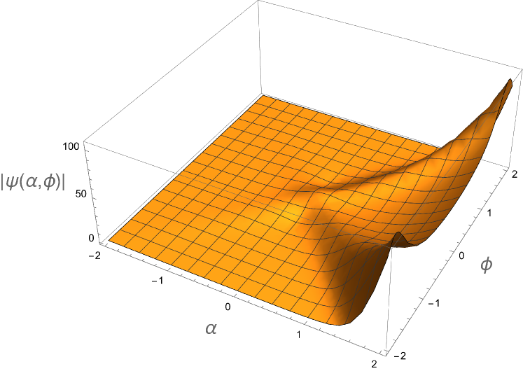
Figure 1: The amplitude of $\psi(\alpha,\phi)=e^{\frac{3}{2}\alpha}\int dq~{}e^{-\frac{1}{2\Delta^{2}}q^{2}}e^{iq\phi+i\epsilon_{q}\alpha}$ with $\Delta=5$, which is a gauge invariant state of Eq. (3) for $\rho(\alpha)=0$. The peak along the classical trajectories of $\phi=\pm\alpha$ is superimposed with an exponentially growing factor of $\alpha$.

The second issue is the directedness of time. The gradual projection of the wave function is a result of a stochastic evolution along the gauge orbit. Under such an evolution, a state usually diffuses in all directions in the gauge orbit. If one of the variables is used as a clock, the diffusion would create a state that is merely more spread over a more extensive range of past and future without pushing time in one direction. In the present case, however, a directedness of time evolution can arise because $\hat{H}$ is asymmetric in $\alpha$. In particular, the kinetic terms in Eq. (3) are exponentially suppressed at large $\alpha$. This can be viewed as the $\alpha$-dependent effective masses, which tend to make the dynamics slower as the universe gets bigger. Since the random walk is exponentially slowed down at large $\alpha$, configurations generated through the random walk at a larger scale factor add up with a stronger constructive interference in the ensemble of Eq. (1). This $\alpha$-dependent effective mass makes the state evolve preferably toward the one with larger $\alpha$ with increasing $T$. For the same reason, gauge invariant states can have exponentially larger amplitude at larger $\alpha$, as is shown in Fig. 1. A projection of $\Psi_{0}$ with finite support in $\alpha$ toward such gauge invariant states makes $\Psi_{0}$ evolve toward the region of large $\alpha$ to maximize the overlap.

Now, we demonstrate the unitarity and directedness of the time evolution through an explicit calculation. We write eigenstates of Eq. (3) with eigenvalue $E$ as $\Psi_{E,q}(\alpha,\phi)=e^{iq\phi+\frac{3}{2}\alpha}f_{E,q}(\alpha)$, where $f_{E,q}(\alpha)$ satisfies

$$f^{{}^{\prime\prime}}_{E,q}(\alpha)+P_{E,q}(\alpha)^{2}f_{E,q}(\alpha)=0,$$ (8)

where

$$P_{E,q}(\alpha)^{2}=q^{2}+(3/2)^{2}+\rho(\alpha)e^{6\alpha}-Ee^{3\alpha}.$$ (9)

For simplicity, we focus on states with $q\lesssim 1$, and assume that there exists a hierarchy among different types of energy densities such that $(\Lambda_{1}/\Lambda_{0})^{1/2}\gg\Lambda_{m}/\Lambda_{1}\gg\Lambda_{r}/\Lambda_{m}\gg 1/\Lambda_{r}^{1/2}\gg 1$. In this case, the evolution undergoes a series of crossovers at $\alpha_{A}\sim\log(1/\Lambda_{r}^{1/2})$, $\alpha_{B}\sim\log(\Lambda_{r}/\Lambda_{m})$ and $\alpha_{C}\sim\log(\Lambda_{m}/\Lambda_{1})$. Between these crossover scales, one of the terms dominates the energy density in Eq. (9), which results in the following epochs: 1) pre-radiation era ($\alpha\ll\alpha_{A})$, 2) radiation-dominated era ($\alpha_{A}\ll\alpha\ll\alpha_{B})$, 3) matter-dominated era, ($\alpha_{B}\ll\alpha\ll\alpha_{C})$, 4) dark-energy-dominated era ($\alpha_{C}\ll\alpha)$. The dark-energy-dominated era is further divided into two sub-eras around $\alpha^{*}\sim\frac{1}{2}\log(\Lambda_{1}/\Lambda_{0})$, depending on whether the $\Lambda_{1}$ or $\Lambda_{0}$ term dominates the dark energy. Below, we describe the evolution of the universe in each era.

II.1 Pre-radiation era

In this era, the Hamiltonian constraint becomes ${\cal H}=\Bigl{\llbracket}e^{-3\alpha}\left(\partial_{\alpha}^{2}-\partial_{\phi}^{2}\right)\Bigl{\rrbracket}$. This may not describe the realistic pre-radiation era as it ignores other effects, such as inflation. Nonetheless, we study this as a toy model because the exact solution available in this limit is useful for demonstrating the general idea without an approximation. Normalizable eigenstates of ${\cal H}$ have non-positive eigenvalues. Eigenstates with eigenvalue $E$ ($E\leq 0$), which are regular in the small $|E|$ limit, are given by

$$\Psi_{E,q}^{(\pm)}(\alpha,\phi) = e^{\frac{3}{2}\alpha+iq\phi}(-E)^{\mp i\frac{\epsilon_{q}}{3}}~{}J\left[\pm i\frac{2}{3}\epsilon_{q};\frac{2}{3}\sqrt{-E}e^{\frac{3}{2}\alpha}\right],~{}~{}~{}~{}~{}~{}$$ (10)

where $J[\nu;z]$ is the Bessel function of the first kind of order $\nu$ and $\epsilon_{q}=\sqrt{q^{2}+\left(\frac{3}{2}\right)^{2}}$. In the small $|E|$ limit, Eq. (10) reduces to gauge-invariant states: $\lim_{E\rightarrow 0}\Psi_{E,q}^{(\pm)}(\alpha,\phi)\sim e^{\frac{3}{2}\alpha}e^{iq\phi\pm i\epsilon_{q}\alpha}$. A general normalizable gauge non-invariant state can be written as

$$\Psi_{0}(\alpha,\phi) = \sum_{s=\pm}\int_{-\infty}^{0}dE\int dq~{}\Phi_{s}(E,q)\Psi_{E,q}^{(s)}(\alpha,\phi).~{}~{}$$ (11)

For $\Phi_{\pm}(E,q)$ that is smooth in $E$, Eq. (6) at large $T$ becomes

$$\Psi(T)=\sum_{s=\pm}\int dq~{}\Phi_{s}(0,q)e^{iq\phi+is\epsilon_{q}\alpha}\chi_{q,s}\left(\frac{e^{\alpha}}{T^{1/3}}\right)+O(1/T),~{}$$ (12)

where $\chi_{q,\pm}(z)=6^{\mp i\frac{2\epsilon_{q}}{3}}\frac{\pi^{1/2}}{2}z^{\frac{3}{2}}\Bigg{[}~{}_{0}\tilde{F}_{2}\left(;\frac{3\pm 2i\epsilon_{q}}{6},\frac{3\pm i\epsilon_{q}}{3};\frac{z^{6}}{648}\right)$ $-\frac{\sqrt{2}}{36}~{}_{1}\tilde{F}_{3}\left(1;\frac{3}{2},\frac{3\pm i\epsilon_{q}}{3},\frac{9\pm 2i\epsilon_{q}}{6};\frac{z^{6}}{648}\right)z^{3}\Bigg{]}$ with ${}_{p}\tilde{F}_{p^{\prime}}\left({a_{1},..,a_{p}};{b_{1},..,b_{p^{\prime}}};x\right)=\frac{{}_{p}F_{p^{\prime}}\left({a_{1},..,a_{p}};{b_{1},..,b_{p^{\prime}}};x\right)}{\Gamma(b_{1})..\Gamma(b_{p^{\prime}})}$.

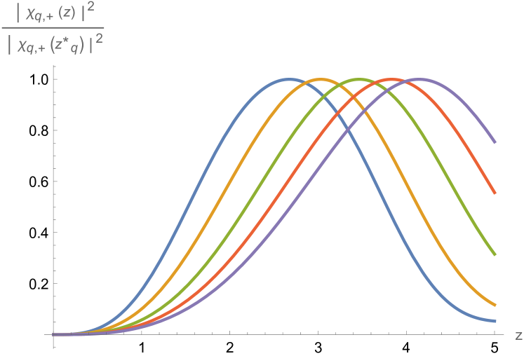
Figure 2: $|\chi_{q,\pm}(z)|^{2}$ normalized by its peak value at $z_{q}^{*}$ with increasing $q=0,2,4,6,8$ from left to right curves. The scale factor at which the wavefunction is peaked increases with $q$ because a larger momentum of $\phi$ gives rise to a larger momentum for $\alpha$.

Eq. (12) describes the evolution of the state as it gradually collapses toward a gauge invariant state with increasing $T$ which is regarded as time. $\chi_{q,\pm}(z)$, which controls the magnitude of the wavefunction for each component of $q$, is peaked at $z_{q}^{*}$, as is shown in Fig. 2. The wavefunction for $\alpha$ is peaked at $T$-dependent scale factor $\alpha(T)$ with a finite uncertainty. At time $T$, $e^{\alpha(T)}\sim T^{1/3}$, and its conjugate momentum is $p_{\alpha}(T)\approx\pm\epsilon_{q}$. While $\Psi(\alpha,\phi;T)$ is not gauge invariant, it satisfies the Hamiltonian constraint at the semi-classical level. Since the state of $\alpha$ is fixed at each $T$, $\alpha$ is not an independent dynamical variable. The scalar, which retains information about the initial state, is the physical degree of freedom. Therefore, the present theory keeps the same number of physical degrees of freedom as the system in which the gauge symmetry is strictly enforced.

For $T\gg 1$, the norm of the wavefunction is independent of $T$ and the resulting unitary time evolution can be written as $\Psi(\alpha,\phi;T+\Delta T)=e^{-i\Delta T\hat{H}_{eff}(T)}\Psi(\alpha,\phi;T)$, where $\hat{H}_{eff}(T)=\frac{1}{3T}\Bigl{\llbracket}\hat{p}_{\alpha}-\hat{\Pi}\sqrt{\hat{p}_{\phi}^{2}+\left(\frac{3}{2}\right)^{2}}\Bigl{\rrbracket}$ is the effective Hamiltonian. Here, $\hat{\Pi}$ is the operator that takes eigenvalues $\pm 1$ for $\psi^{(\pm)}_{E,q}$. The effective Hamiltonian makes $\alpha$ to increase with increasing time irrespective of $p_{\alpha}$. This arrow of time arises because the preferred direction of the gauge parameter is determined by the state: for states with $p_{\alpha}>0$ ($p_{\alpha}<0$), $e^{i\epsilon\hat{H}}$ ($e^{-i\epsilon\hat{H}}$) generates a stronger constructive interference to always push the state to larger $\alpha$.

II.2 Radiation and matter-dominated eras

At $T_{A}=1/\Lambda_{r}^{3/2}$, the peak of the wavefunction reaches the first crossover scale: $\alpha(T_{A})\sim\alpha_{A}$. For $T>T_{A}$, the evolution becomes dominated by radiation and then matter consecutively. We consider the two eras together because the analysis is parallel for those two cases. In each era, we can keep only one dominant term in the energy density to write Eq. (9) as

$$P_{E,q}(\alpha)^{2}=C_{n}e^{n\alpha}-Ee^{3\alpha}$$ (13)

with $C_{2}=\Lambda_{r}$ and $C_{3}=\Lambda_{m}$, respectively. In solving Eq. (9), it is useful to understand the relative magnitude between the two terms in Eq. (13) for typical values that $E$ and $\alpha$ take. At time $T$, the range of $E$ in Eq. (6) is $E(T)\sim T^{-1}$ while the wavefunction is peaked at $\alpha(T)$. At $T_{A}$, the two terms are comparable: $\frac{C_{2}e^{2\alpha(T_{A})}}{E(T_{A})e^{3\alpha(T_{A})}}\sim\Lambda_{r}e^{2\alpha_{A}}\sim 1$. For $T\gg T_{A}$, a hierarchy emerges such that

$$C_{n}e^{n\alpha(T)}\gg E(T)e^{3\alpha(T)}\gg 1.$$ (14)

This will be shown to be true through a self-consistent computation in the following. For now, we proceed, assuming that this is the case. With $P_{E,q}\gg 1$, we can use the WKB-approximation to write the eigenstates of ${\cal H}$ with eigenvalue $E$ as

$$\Psi_{E,q}^{(s)}(\alpha,\phi)=e^{\frac{3}{2}\alpha+iq\phi}\frac{\exp{\left[is\int P_{E,q}(\alpha)d\alpha\right]}}{\sqrt{P_{E,q}(\alpha)}}$$ (15)

with $s=\pm 1$. Furthermore, Eq. (14) allows us to expand Eq. (15) around $E=0$ to write $\Psi_{E,q}^{(\pm)}(\alpha,\phi)\approx\frac{e^{\frac{3}{2}\alpha+i\left[q\phi\pm\int P_{0,q}(\alpha)d\alpha\mp E\int\frac{e^{3\alpha}}{2P_{0,q}(\alpha)}d\alpha\right]}}{\sqrt{P_{0,q}(\alpha)}}$. To the leading order in $1/T$, the integration over $E$ in Eq. (6) leads to

$$\Psi(T) = \sum_{s=\pm}\int dq~{}\Phi_{s}(0,q)e^{i\left(q\phi+2s\frac{\sqrt{C_{n}}}{n}e^{\frac{n}{2}\alpha}\right)}\times$$ (16)

$$\chi_{n}\left(\frac{e^{\alpha}}{(C_{n}T^{2})^{\frac{1}{6-n}}}\right),$$

where $\chi_{n}(z)=z^{\frac{6-n}{4}}e^{-\frac{z^{6-n}}{2(6-n)^{2}}}$. At time $T$, the wavefunction is peaked at $e^{\alpha(T)}\sim(C_{n}T^{2})^{\frac{1}{6-n}}$. In the radiation-dominated era, the size of the universe increases as $e^{\alpha(T)}\sim e^{\alpha_{A}}\left(T/T_{A}\right)^{\frac{1}{2}}$ until $\alpha(T)$ reaches $\alpha_{B}$ around $T_{B}\sim\Lambda_{r}^{3/2}/\Lambda_{m}^{2}$. In $T\gg T_{B}$, the matter dominates and the universe expands as $e^{\alpha(T)}\sim e^{\alpha_{B}}\left(T/T_{B}\right)^{\frac{2}{3}}$. We note that Eq. (14) is indeed satisfied throughout the radiation-dominated era and afterward because $\frac{C_{n}e^{n\alpha(T)}}{E(T)e^{3\alpha(T)}}\sim\frac{C_{n}e^{n\alpha(T)}}{C_{n}^{1/2}e^{3\alpha(T)-\frac{6-n}{2}\alpha(T)}}\sim\left(C_{n}e^{n\alpha(T)}\right)^{1/2}\gg 1$ for $T\gg T_{A}$. Therefore, the approximation used in Eq. (16) is justified. In these eras, the effective Hamiltonian is given by

$$\hat{H}_{eff}(T)=\frac{2}{(6-n)T}\Bigl{\llbracket}\hat{p}_{\alpha}-\sqrt{C_{n}}\hat{\Pi}e^{\frac{n}{2}\hat{\alpha}}\Bigl{\rrbracket}$$ (17)

to the leading order in $e^{-\alpha}$, where $\hat{\Pi}$ is an operator that takes eigenvalue $s$ for $\Psi_{E,q}^{(s)}(\alpha,\phi)$. In the regime where the WKB approximation is valid, $\hat{\Pi}\approx\hat{p}_{\alpha}/|\hat{p}_{\alpha}|$. The effective Hamiltonian does not depend on $q$ to the leading order in $e^{-\alpha}$.

II.3 Dark-energy-dominated era

Around time $T_{C}\sim\Lambda_{m}/\Lambda_{1}^{3/2}$, the wavefunction becomes peaked at $\alpha_{C}$. Beyond this size, the dark energy dominates and Eq. (15) becomes

$$\Psi_{E,q}(\alpha,\phi)=\frac{e^{\frac{3}{2}\alpha}e^{i\left(q\phi\pm\eta(\alpha)\mp E\xi(\alpha)\right)}}{\left[\Lambda_{0}e^{6\alpha}+\Lambda_{1}e^{4\alpha}\right]^{1/4}},$$ (18)

where $\eta(\alpha)=\frac{e^{2\alpha}}{3}\frac{\Lambda_{0}^{2}e^{4\alpha}+3\Lambda_{0}\Lambda_{1}e^{2\alpha}+3\Lambda_{1}^{2}}{\left(\Lambda_{0}e^{2\alpha}+\Lambda_{1}\right)^{3/2}+\Lambda_{1}^{3/2}}$, $\xi(\alpha)=\frac{1}{4\sqrt{\Lambda_{0}}}\log\left[\frac{\left(\sqrt{\Lambda_{0}e^{2\alpha}}+\sqrt{\Lambda_{0}e^{2\alpha}+\Lambda_{1}}\right)^{2}}{\Lambda_{1}}\right]$. The soft projection gives the time-dependent wavefunction,

$$\Psi(T)=\frac{e^{\frac{3}{2}\alpha}}{\sqrt{T}}\sum_{s=\pm}\int dq~{}\Phi_{s}(0,q)\frac{e^{i\left(q\phi+s\eta(\alpha)\right)}e^{-\frac{\xi(\alpha)^{2}}{2T^{2}}}}{\left[\Lambda_{0}e^{6\alpha}+\Lambda_{1}e^{4\alpha}\right]^{1/4}}.$$ (19)

In the first part of the dark-energy-dominated era, $\Lambda_{0}$ is negligible, and Eq. (19) reduces to Eq. (16) with $n=4$ and $C_{4}=\Lambda_{1}$. In this era, the universe expands as $e^{\alpha(T)}\sim e^{\alpha_{C}}(T/T_{C})$, and its unitary evolution is governed by Eq. (17) for $n=4$.

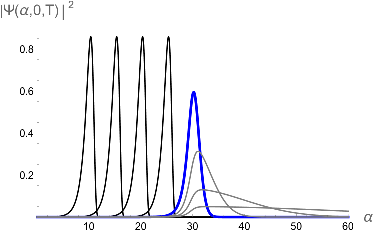
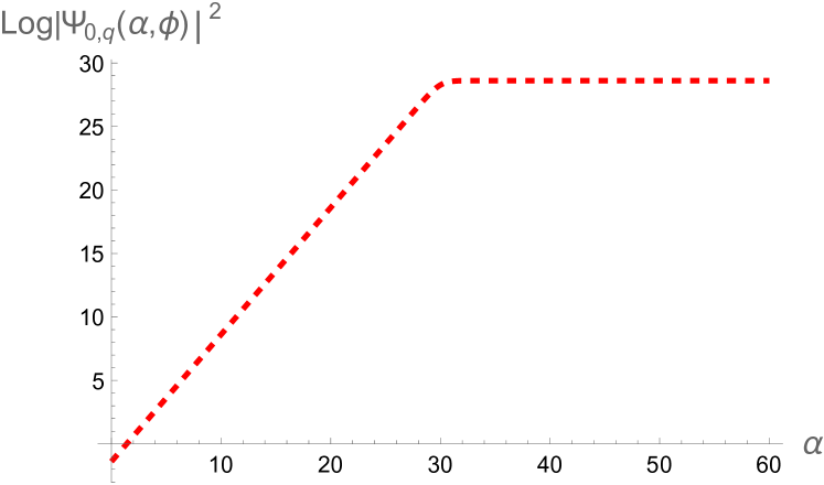
Figure 3: (a) The amplitude of the wavefunction in the dark-energy-dominated era with $\Lambda_{1}=1$, $\Lambda_{0}=e^{-60}$ and $\Phi_{+}(0,q)=\delta(q)$, $\Phi_{-}(0,q)=0$. Each curve represents $|\Psi(\alpha,0,T)|^{2}$ as a function of $\alpha$ for $T=e^{10},e^{15},e^{20},e^{25},e^{30},e^{31},^{32},e^{33}$ from left to right. The curve in the thick (blue) line is at $T^{*}=e^{30}$, which marks the crossover from the $\Lambda_{1}$-dominated to the $\Lambda_{0}$-dominated evolution. At the crossover time, the wavefunction is peaked around $\alpha^{*}=30$. For $T<T^{*}$, the peak of the wavefunction moves to larger values of $\alpha$ with increasing $T$. Beyond $T^{*}$, the wavefunction gets broader in $T$ with the peak position fixed at $\alpha^{*}$. (b) The logarithm of the amplitude of the gauge invariant wavefunction $\Psi_{E=0,q}(\alpha,\phi)$ in Eq. (18) for the same choice of parameters as in (a).

At $T^{*}=\Lambda_{0}^{-1/2}$, the evolution crossovers to the $\Lambda_{0}$-dominated era and the wavefunction is peaked around $\alpha^{*}\equiv\frac{1}{2}\log\frac{\Lambda_{1}}{\Lambda_{0}}$. In $T\gg T^{*}$, the form of the wavefunction becomes qualitatively different. In $\alpha\ll\alpha^{*}$, it is still described by Eq. (16) with $n=4$. In $\alpha\gg\alpha^{*}$, however, the wavefunction becomes

$$\Psi(T)=T^{-1/2}\Lambda_{0}^{-\frac{1}{4}}\times$$

$$\sum_{s=\pm}\int dq~{}\Phi_{s}(0,q)e^{i\left(q\phi+s\frac{\sqrt{\Lambda_{0}}}{3}e^{3\alpha}\right)}e^{-\frac{\left(\alpha-\alpha^{*}\right)^{2}}{8\Lambda_{0}T^{2}}}.$$ (20)

As is shown in Fig. 3, the peak of the wavefunction is pinned at $\alpha^{*}$, and the width grows as $\Delta\alpha\sim T$ on the side of $\alpha>\alpha^{*}$. While the expectation value of $e^{\alpha}$ grows exponentially in $T$, the wavefunction acquires an increasingly large uncertainty of $\alpha$. In this era, the effective Hamiltonian, which can be written as $\hat{H}_{eff}(T)=\frac{1}{T}\Bigl{\llbracket}(\hat{\alpha}-\alpha^{*})\left(\hat{p}_{\alpha}-\sqrt{\Lambda_{0}}e^{3\hat{\alpha}}\hat{\Pi}\right)\Bigl{\rrbracket}$ in $\alpha\gg\alpha^{*}$, describes the broadening of the wavefunction. Therefore, the semi-classical time evolution ends once the $\alpha$-independent cosmological constant dominates. The change in the character of the time evolution in the $\Lambda_{0}$-dominated era can be understood from the profile of gauge-invariant wavefunction. For $\alpha<\alpha^{*}$, the gauge-invariant wavefunction $\Psi_{E=0,q}(\alpha,\phi)$ in Eq. (18) grows exponentially in $\alpha$ as is shown in Fig. 3. If an initial wavefunction is localized in $\alpha<\alpha^{*}$, the projection $e^{-\frac{T^{2}}{2}\hat{H}^{2}}$ pushes the wavefunction to the region with larger amplitude to maximize the overlap, which gives rise to the directed semi-classical time evolution. On the other hand, the amplitude of $\Psi_{E=0,q}(\alpha,\phi)$ becomes flat in $\alpha>\alpha^{*}$, and the projection makes the wavefunction evolve diffusively.

III Discussion

In the present proposal, the time evolution is one big measurement that causes a gauge non-invariant state of an instant to gradually collapse toward a gauge-invariant state. The wavefunction collapse is not only an intrinsic part of time evolutionGhirardi et al. (1986, 1990); Diósi (1989); Penrose (1996) but is the very driving force. Time flows toward the direction that maximizes the overlap between the instantaneous state and a gauge-invariant state. Therefore, the violation of the Hamiltonian constraint at the quantum level plays the role of an absolute time. A prediction that follows is that the expectation value of $\hat{H}^{2}$, which is in principle measurable, is non-zero for our vacuum, and decreases monotonically with time as $\langle\Psi(T)|\hat{H}^{2}|\Psi(T)\rangle\sim T^{-2}$.

Appendix A Failed emergence of Coulomb phase from a soft non-compact gauge constraint

In models that exhibit emergent gauge symmetry, the full Hilbert space of microscopic degrees of freedom includes states that do not satisfy Gauss’s constraint. Nonetheless, gauge theories can dynamically emerge at low energies in the presence of interactions that energetically penalize states that violate the constraint. In this appendix, we review how this works for a compact group and discuss how it fails for the non-compact counterpart.

A.1 U(1) group

Here, we consider a lattice model where the pure U(1) gauge theory emerges at low energies. Let $\hat{\theta}_{i,\mu}$ be the $U(1)$ rotor variable defined on link $(i,\mu)$ of the $d$-dimensional hyper-cubic lattice, where $i$ is the site index and $\mu=1,2,..,d$ denotes $d$ independent directions of links. For links along $-\mu$ direction, we define $\hat{\theta}_{i,-\mu}=-\hat{\theta}_{i-\mu,\mu}$. $\hat{n}_{i,\mu}$ denotes the conjugate momentum of $\hat{\theta}_{i,\mu}$. With $\theta_{i,\mu}\sim\theta_{i,\mu}+2\pi$, $\hat{n}_{i,\mu}$ takes integer eigenvalues. The Hamiltonian is written as

$$\hat{H}=U\sum_{i}\hat{Q}_{i}^{2}+g\sum_{i,\mu}\hat{n}_{i,\mu}^{2}+...,$$ (21)

where $\hat{Q}_{i}\equiv\sum_{\mu}(\hat{n}_{i\mu}-\hat{n}_{i-\mu,\mu})$ and $...$ denotes other terms. The first two terms in the Hamiltonian respect the local $U(1)$ symmetry for every link, but $...$ may partially or completely break the symmetry. For example, we add $\hat{H}_{J}=-2J\sum_{i,\mu}\cos(\hat{\theta}_{i,\mu})$ that breaks all internal symmetry. We are interested in the low-energy spectrum of the theory in the limit that $U$ is larger than all other couplings. If we view $\hat{n}_{i,\mu}$ as the electric flux in direction $\mu$, $\hat{Q}_{i}$ corresponds to the divergence of the electric field evaluated at site $i$. The $U$-term in the Hamiltonian penalizes states that violate Gauss’s constraint. In the $U\rightarrow\infty$ limit, Gauss’s constraint is strict, and states with finite energies only have closed loops of electric flux lines.

For a finite $U$, Gauss’s constraint is not strictly enforced. However, the gap between the low-energy sector with energy $E\ll U$ and the sector with $E\sim U$ guarantees that the low-energy Hilbert space evolves adiabatically as $U$ is decreased from infinity to a finite value as long as $U$ is much larger than other couplings. Therefore, there remains a one-to-one correspondence between states with $Q_{i}=0$ and the states with $E\ll U$ for a large enough $U$. This guarantees that there exists a unitary transformation $\hat{V}$ that rotates the basis such that the Hamiltonian has no off-diagonal elements that mix the $Q_{i}=0$ sector and the rest. In the rotated basis, Gauss’s law becomes an exact constraint within the low-energy Hilbert space with $E\ll U$. Using the standard degenerate perturbation theory, one can derive the pure U(1) gauge theory as the low-energy effective Hamiltonian,

$$\hat{V}\hat{H}\hat{V}^{\dagger}=g\sum_{i,\mu}\hat{n}_{i,\mu}^{2}-\sum_{C}t_{C}\cos\left(\sum_{(i,\mu)\in C}\hat{\theta}_{i,\mu}\right),$$ (22)

where $t_{C}\sim J(J/U)^{L_{C}-1}$ with $L_{C}$ being the length of closed loop $C$. For $g\ll t_{\Box}$, the gauge theory is in the deconfinement phase that supports $(d-1)$ gapless photons. The gaplessness of the photon is protected from small perturbations. Therefore, the Coulomb phase emerges through the soft Gauss constraint for the U(1) group.

A.2 $R$ group

Now, we consider a non-compact counterpart of Eq. (21) by replacing $\theta_{i,\mu}$ with a non-compact variable $\hat{x}_{i,\mu}$,

$$\hat{H}=U\sum_{i}\hat{Q}_{i}^{2}+g\sum_{i,\mu}\hat{p}_{i,\mu}^{2}+....$$ (23)

Here, $\hat{p}_{i,\mu}$ denotes the conjugate momentum of $\hat{x}_{i,\mu}$. Their eigenvalues can take any real number. $\hat{Q}_{i}\equiv\sum_{\mu}(\hat{p}_{i\mu}-\hat{p}_{i-\mu,\mu})$ is the generator of a local $R$ transformation at site $i$. The symmetry-breaking perturbation, which is included in $...$, is written as $\hat{H}_{J}=J\sum_{i,\mu}\hat{x}_{i,\mu}^{2}$. The question is whether the local $R$ symmetry emerges at a large but finite $U$ in the presence of such perturbations. For simplicity, let us consider only $\hat{H}_{J}$ in the perturbation, which is enough for our purpose. In this case, the theory is quadratic and can be exactly solved. In the Fourier space, we write $\left(\begin{array}[]{c}\hat{x}_{i,\mu}\\ \hat{p}_{i,\mu}\end{array}\right)=\frac{1}{\sqrt{L^{d}}}\sum_{m}\sum_{k}\left(\begin{array}[]{c}\hat{x}_{k}^{(m)}\\ \hat{p}_{k}^{(m)}\end{array}\right)\varepsilon_{k,\mu}^{(m)}~{}e^{ir_{i}k}$, where $k=\frac{2\pi}{L}(l_{1},..,l_{d})$ with $l_{i}=-L/2,..,L/2-1$ denotes discrete momenta that are compatible with the periodic boundary condition for the system with linear size $L$. $\varepsilon_{k,\mu}^{(m)}$ with $m=1,..,d$ denotes the polarization of the $m$-th mode with $\varepsilon_{k,\mu}^{(m)*}\varepsilon_{k,\mu}^{(n)}=\delta_{m,n}$. In terms of the Fourier mode, the Hamiltonian becomes diagonal,

$$\hat{H}=\sum_{k,m}\left[J\hat{x}_{k}^{(m)}\hat{x}_{-k}^{(m)}+V_{k,m}\hat{p}_{k}^{(m)}\hat{p}_{-k}^{(m)}\right],$$ (24)

where $V_{k,1}=g+4U\sum_{\mu}\sin^{2}\frac{k_{\mu}}{2}$ and $V_{k,m\geq 2}=g$. Here, $m=1$ represents the longitudinal mode with $\varepsilon_{k,\mu}^{(1)}=\frac{e^{\frac{i}{2}k_{\mu}}\sin\left(\frac{k_{\mu}}{2}\right)}{\sqrt{\sum_{\nu}\sin^{2}\left(\frac{k_{\nu}}{2}\right)}}$, and $2\leq m\leq d$ represent $(d-1)$ transverse modes. The energy dispersion of the mode is given by $E_{k,m}=2\sqrt{JV_{k,m}}$. It is noted that all excitations are gapped for any $J,g>0$. Therefore, there is no gapless photon.

The failed emergence of the Coulomb phase is a consequence of the fact that the states with $Q_{i}=0$ are in the middle of the spectrum with continuously varying $Q_{i}$. Because there is no gap between the gauge invariant states and others, an arbitrarily small perturbation mixes states with different eigenvalues with an $O(1)$ weight. It destroys the one-to-one correspondence between the gauge invariant states and the low-energy states for any non-zero $J/U$. This can also be understood in terms of the ground state,

$$\langle x|\psi_{0}\rangle=e^{-\frac{1}{2}\sum_{k,m}\sqrt{\frac{J}{V_{k,m}}}\left|x_{k}^{(m)}\right|^{2}}.$$ (25)

In the thermodynamic limit, the trace distance between the ground state and the state obtained by applying a local $R$ transformation $e^{iy\hat{Q}_{0}}$ at the origin is

$$d_{\psi_{0}}(y) = \sqrt{1-e^{-2y^{2}\int\frac{dk}{(2\pi)^{d}}\sqrt{\frac{J}{g+4U\sum_{\mu}\sin^{2}\frac{k_{\mu}}{2}}}\sum_{\nu}\sin^{2}\frac{k_{\nu}}{2}}}.$$ (26)

As expected, only the longitudinal modes contribute to the trace distance. Due to the soft longitudinal mode, there always exists $y$ for which Eq. (26) becomes $O(1)$ for any $J/U\neq 0$.

Appendix B Reduced FRW model

In principle, we should treat all degrees of freedom on an equal footing. Let us write the full Hamiltonian as

$$\hat{H}=\Bigl{\llbracket}e^{-3\hat{\alpha}}(-\hat{p}_{\alpha}^{2}+\hat{p}_{\phi}^{2})+\hat{h}_{X}\Bigl{\rrbracket}.$$ (27)

Here, $X$ collectively represents all other degrees of freedom that include radiation, matter and other fields that source the dark energy and $\hat{h}_{X}=h(\hat{\alpha},\hat{X},\hat{p}_{X})$ denotes the Hamiltonian that governs their dynamics. Let $|X(\alpha)\rangle$ be an eigenstate of $\hat{h}_{X}$ with energy density $\rho_{0}(\alpha)$ at each scale factor $\alpha$: $\hat{h}_{X}|X(\alpha)\rangle=e^{3\alpha}\rho_{0}(\alpha)|X(\alpha)\rangle$. Now, we consider a sub-Hilbert space defined by the projection operator,

$$\hat{\cal P}=\int d\alpha d\phi~{}|\alpha,\phi\rangle\langle\alpha,\phi|,$$ (28)

where $|\alpha,\phi\rangle\equiv|\alpha\rangle\otimes|\phi\rangle\otimes|X(\alpha)\rangle$. For $|\Psi\rangle=\int d\alpha d\phi~{}\Psi(\alpha,\phi)|\alpha,\phi\rangle$, the Hamiltonian projected to the sub-Hilbert space acts as

$${\cal\hat{P}}\hat{H}|\Psi\rangle=\int d\alpha d\phi~{}\left[{\cal H}\Psi(\alpha,\phi)\right]|\alpha,\phi\rangle,$$ (29)

where

$$\left[{\cal H}\Psi(\alpha,\phi)\right] = \frac{1}{2}\Bigg{\{}\Big{[}e^{-3\alpha}\Big{(}\partial_{\alpha}^{2}+\langle X(\alpha)|\partial_{\alpha}^{2}|X(\alpha)\rangle+2\langle X(\alpha)|\partial_{\alpha}|X(\alpha)\rangle\partial_{\alpha}-\partial_{\phi}^{2}\Big{)}+e^{3\alpha}\rho_{0}(\alpha)\Big{]}+h.c.\Bigg{\}}\Psi(\alpha,\phi),$$ (30)

where $h.c.$ represents the Hermitian conjugate. Without loss of generality, we can choose the phase of $|X(\alpha)\rangle$ such that $\langle X(\alpha)|\partial_{\alpha}|X(\alpha)\rangle=0$ because $\alpha$ is non-compact. With $\rho(\alpha)\equiv\rho_{0}(\alpha)+e^{-6\alpha}\langle\Psi(\alpha)|\partial_{\alpha}^{2}|\Psi(\alpha)\rangle$, we obtain the projected Hamiltonian in Eq. (3),

$${\cal H}=\Bigl{\llbracket}e^{-3\alpha}(\partial_{\alpha}^{2}-\partial_{\phi}^{2})+e^{3\alpha}\rho(\alpha)\Bigl{\rrbracket},$$ (31)

where $\rho(\alpha)$ behaves as an $\alpha$-dependent energy density contributed from $X$ degrees of freedom.

References

- Rovelli (2002) C. Rovelli, Phys. Rev. D 65, 124013 (2002), URL https://link.aps.org/doi/10.1103/PhysRevD.65.124013.
- Dittrich (2007) B. Dittrich, General Relativity and Gravitation 39, 1891 (2007), ISSN 1572-9532, URL https://doi.org/10.1007/s10714-007-0495-2.
- DeWitt (1967) B. S. DeWitt, Phys. Rev. 160, 1113 (1967), URL https://link.aps.org/doi/10.1103/PhysRev.160.1113.
- Isham (1992) C. J. Isham, ArXiv General Relativity and Quantum Cosmology e-prints (1992), eprint gr-qc/9210011.
- Kuchar (1992) K. V. Kuchar, Proceedings of the 4th Canadian Conference on General Relativity and Relativistic Astrophysics p. 211 (1992).
- Anderson (2012) E. Anderson, Annalen der Physik 524, 757 (2012), eprint https://onlinelibrary.wiley.com/doi/pdf/10.1002/andp.201200147, URL https://onlinelibrary.wiley.com/doi/abs/10.1002/andp.201200147.
- Page and Wootters (1983) D. N. Page and W. K. Wootters, Phys. Rev. D 27, 2885 (1983), URL https://link.aps.org/doi/10.1103/PhysRevD.27.2885.
- Lee (2021) S.-S. Lee, Journal of High Energy Physics 2021, 204 (2021), URL https://doi.org/10.1007/JHEP04(2021)204.
- Barbour and Foster (2008) J. Barbour and B. Z. Foster, arXiv e-prints arXiv:0808.1223 (2008), eprint 0808.1223.
- Silvia De Bianchi (2024) L. M. Silvia De Bianchi, Marco Forgione, ed., Time and Timelessness in Fundamental Physics and Cosmology (Springer Cham, 2024).
- Horwitz et al. (1988) L. P. Horwitz, R. I. Arshansky, and A. C. Elitzur, Foundations of Physics 18, 1159 (1988), URL https://doi.org/10.1007/BF01889430.
- Ishibashi et al. (1997) N. Ishibashi, H. Kawai, Y. Kitazawa, and A. Tsuchiya, Nuclear Physics B 498, 467 (1997), ISSN 0550-3213, URL https://www.sciencedirect.com/science/article/pii/S0550321397002903.
- Connes and Rovelli (1994) A. Connes and C. Rovelli, Classical and Quantum Gravity 11, 2899 (1994), URL https://dx.doi.org/10.1088/0264-9381/11/12/007.
- Smolin (2015) L. Smolin, Studies in History and Philosophy of Science Part B: Studies in History and Philosophy of Modern Physics 52, 86 (2015), ISSN 1355-2198, cosmology and Time: Philosophers and Scientists in Dialogue, URL https://www.sciencedirect.com/science/article/pii/S1355219815000271.
- Carroll and Chen (2004) S. M. Carroll and J. Chen (2004), eprint hep-th/0410270.
- Magueijo (2021) J. Magueijo, Physics Letters B 820, 136487 (2021), ISSN 0370-2693, URL https://www.sciencedirect.com/science/article/pii/S0370269321004275.
- Hull and Lambert (2014) C. M. Hull and N. Lambert, Journal of High Energy Physics 2014, 16 (2014), URL https://doi.org/10.1007/JHEP06(2014)016.
- Lee (2020) S.-S. Lee, Journal of High Energy Physics 2020, 70 (2020), URL https://doi.org/10.1007/JHEP06(2020)070.
- Leutheusser and Liu (2023) S. Leutheusser and H. Liu, Phys. Rev. D 108, 086020 (2023), URL https://link.aps.org/doi/10.1103/PhysRevD.108.086020.
- Brahma et al. (2022) S. Brahma, R. Brandenberger, and S. Laliberte, Journal of High Energy Physics 2022, 31 (2022), URL https://doi.org/10.1007/JHEP09(2022)031.
- Kitaev (2006) A. Kitaev, Annals of Physics 321, 2 (2006), ISSN 0003-4916, january Special Issue, URL https://www.sciencedirect.com/science/article/pii/S0003491605002381.
- Wen (2003) X.-G. Wen, Phys. Rev. Lett. 90, 016803 (2003), URL https://link.aps.org/doi/10.1103/PhysRevLett.90.016803.
- Hermele et al. (2004) M. Hermele, M. P. A. Fisher, and L. Balents, Phys. Rev. B 69, 064404 (2004), URL https://link.aps.org/doi/10.1103/PhysRevB.69.064404.
- Maldacena (1999) J. M. Maldacena, Int.J.Theor.Phys. 38, 1113 (1999), eprint hep-th/9711200.
- Witten (1998) E. Witten, Adv.Theor.Math.Phys. 2, 253 (1998), eprint hep-th/9802150.
- Gubser et al. (1998) S. Gubser, I. R. Klebanov, and A. M. Polyakov, Phys.Lett. B428, 105 (1998), eprint hep-th/9802109.
- de Boer et al. (2000) J. de Boer, E. P. Verlinde, and H. L. Verlinde, JHEP 0008, 003 (2000), eprint hep-th/9912012.
- Skenderis (2002) K. Skenderis, Class.Quant.Grav. 19, 5849 (2002), eprint hep-th/0209067.
- Lee (2014) S.-S. Lee, Journal of High Energy Physics 2014, 76 (2014), ISSN 1029-8479, URL https://doi.org/10.1007/JHEP01(2014)076.
- Lee (2016) S.-S. Lee, Journal of High Energy Physics 2016, 44 (2016), ISSN 1029-8479, URL https://doi.org/10.1007/JHEP09(2016)044.
- Özer and Taha (1987) M. Özer and M. Taha, Nuclear Physics B 287, 776 (1987), ISSN 0550-3213, URL https://www.sciencedirect.com/science/article/pii/0550321387901283.
- Freese et al. (1987) K. Freese, F. C. Adams, J. A. Frieman, and E. Mottola, Nuclear Physics B 287, 797 (1987), ISSN 0550-3213, URL https://www.sciencedirect.com/science/article/pii/0550321387901295.
- Carvalho et al. (1992) J. C. Carvalho, J. A. S. Lima, and I. Waga, Phys. Rev. D 46, 2404 (1992), URL https://link.aps.org/doi/10.1103/PhysRevD.46.2404.
- Chen and Wu (1990) W. Chen and Y.-S. Wu, Phys. Rev. D 41, 695 (1990), URL https://link.aps.org/doi/10.1103/PhysRevD.41.695.
- Ghirardi et al. (1986) G. C. Ghirardi, A. Rimini, and T. Weber, Phys. Rev. D 34, 470 (1986), URL https://link.aps.org/doi/10.1103/PhysRevD.34.470.
- Ghirardi et al. (1990) G. C. Ghirardi, P. Pearle, and A. Rimini, Phys. Rev. A 42, 78 (1990), URL https://link.aps.org/doi/10.1103/PhysRevA.42.78.
- Diósi (1989) L. Diósi, Phys. Rev. A 40, 1165 (1989), URL https://link.aps.org/doi/10.1103/PhysRevA.40.1165.
- Penrose (1996) R. Penrose, General Relativity and Gravitation 28, 581 (1996), URL https://doi.org/10.1007/BF02105068.