A Unified Theory of Quantum Neural Network Loss Landscapes

Abstract

Classical neural networks with random initialization famously behave as Gaussian processes in the limit of many neurons, with the architecture of the network determining the covariance of the associated process. This limit allows one to completely characterize the training behavior of such networks and show that, generally, classical neural networks train efficiently via gradient descent. No such general understanding exists for quantum neural networks (QNNs), which—outside of certain special cases—are known to not behave as Gaussian processes when randomly initialized.

We here prove that instead QNNs and their first two derivatives generally form what we call Wishart processes, where now certain algebraic properties of the network determine the hyperparameters of the process. This Wishart process description allows us to, for the first time:

1. Give necessary and sufficient conditions for a QNN architecture to have a Gaussian process limit.

2. Calculate the full gradient distribution, unifying previously known barren plateau results.

3. Calculate the local minima distribution of algebraically constrained QNNs.

The transition from trainability to untrainability in each of these contexts is governed by a single parameter we call the degrees of freedom of the network architecture. We thus end by proposing a formal definition for the “trainability” of a given QNN architecture using this experimentally accessible quantity.

I Introduction

I.1 Motivation

One of the miracles of machine learning on classical computers is that simple, gradient-based optimizers can efficiently find the minimum of extremely high-dimensional, nonconvex loss landscapes, allowing for the efficient training of deep neural networks. Over the past decade this has been understood in more and more detail via random matrix theory. In particular, it is now known that the loss landscapes of randomly initialized, wide neural networks are distributed as Gaussian processes with covariance given by the so-called neural tangent kernel (NTK) [1, 2, 3, 4]. The NTK is completely determined by the neural structure of the network, linking the asymptotic behavior of the network to architectural choices made in its construction. This understanding of classical neural networks has been used to show that large neural networks train efficiently via gradient descent [2, 3, 5, 6]. It also explains other emergent phenomena in deep learning, such as the remarkably good generalization performance of neural networks beyond what learning theory predicts [5, 7].

One might hope that a similar, universal story would exist for quantum neural networks (QNNs). These are classes of neural networks where the associated loss function $\ell$ takes as input a quantum state $\bm{\rho}$, performs some parameterized unitary operation $\bm{U}$, and then measures some quantum observable $\bm{O}$. That is,

$$\ell\left(\bm{\rho}\right)=\Tr\left(\bm{\rho}\bm{U}^{\dagger}\bm{O}\bm{U}\right).$$ (1)

Such networks are defined by the choice of parameterized gate set $\bm{U}$ (typically called the ansatz) and the observable $\bm{O}$ measured after the ansatz is applied (here called the objective observable) [8]. Unfortunately, it is known that QNNs generally do not have a quantum NTK (QNTK) asymptotic limit. For instance, randomly initialized QNNs with generic shallow ansatzes instead converge to Wishart hypertoroidal random fields (WHRFs) with poor local minima [9, 10]. Though a QNTK limit has been shown to exist in certain specialized settings [11, 12, 13], they all exhibit a superpolynomial decay in gradients known as the barren plateau phenomenon [14]. This implies that measuring the gradient of such a network on a quantum computer would take a superpolynomial number of measurements to resolve. It is therefore unknown whether there exist classes of QNNs which asymptotically converge to Gaussian processes that are usable in practice.

The presence of barren plateaus or poor local minima in QNN loss landscapes paints a pessimistic picture for the practical utility of generic QNNs. However, these negative results can be circumvented by considering structured QNNs. For instance, one might constrain the parameterized ansatz $\bm{U}$ to be generated by a low-dimensional Lie algebra $\mathfrak{g}$ [15]. If the objective observable $\bm{O}$ is itself a representation of an element of $\mathfrak{g}$, the QNN is called a Lie algebra-supported ansatz (LASA). It is known that LASAs do not exhibit barren plateaus when $\bm{\rho}$ and $\mathfrak{g}$ are chosen judiciously [16, 17]. Many of the initial proposals for LASA-based quantum learning algorithms have since been dequantized [18, 19], but there still do exist unconditionally provable quantum advantages in using LASAs for certain learning tasks [20, 21]. Though this is perhaps the most promising direction in QNN research, nothing concretely is known about the loss landscapes of LASAs beyond the variance of the loss function over parameter space.

I.2 Contributions

Fully understanding how the various phenomenologies of QNN loss landscapes are related is important if we ever hope to have as deep an understanding of QNNs as the neural tangent kernel has enabled for classical neural networks. Motivated by this, we here for the first time prove a concise asymptotic limit for the loss functions of effectively all QNNs with approximately uniformly random initialization and problem-independent choice of ansatz. In short, our main result is proving that wide (not necessarily deep) QNNs form Wishart processes. Such processes can be written exactly in terms of the matrix elements of Wishart-distributed positive semidefinite random matrices $\bm{W}$, which are distributed as:

$$\bm{W}=\bm{X}\bm{X}^{\dagger}$$ (2)

for $\bm{X}$ a rectangular matrix with i.i.d. standard normal entries. The number of columns of $\bm{X}$ is called the degrees of freedom $r$ of $\bm{W}$ in analogy with the degrees of freedom of a $\chi^{2}$-distributed random variable; indeed, the diagonal entries of $\bm{W}$ are i.i.d. $\chi^{2}$-distributed each with $r$ degrees of freedom.

Just as the neural structure of a given classical neural network determines its associated neural tangent kernel, the algebraic structure of a QNN completely determines the hyperparameters of its associated Wishart process. This algebraic structure arises from viewing a given ansatz $\bm{U}$ as belonging to the automorphism group of some Jordan algebra—effectively, a Lie algebra with the Lie bracket replaced by the anticommutator—$\mathcal{A}\cong\bigoplus\limits_{\alpha}\mathcal{A}_{\alpha}$ to which the objective observable $\bm{O}$ belongs. We show that such a description exists for any QNN by considering $\bm{O}$ as belonging to a Jordan subalgebra of the space of Hermitian matrices. We call this link between the Jordan algebraic structure of a QNN and its associated Wishart process description a Jordan algebraic Wishart system (JAWS).

Such Jordan subalgebras have been completely classified [22, 23]: each $\mathcal{A}_{\alpha}$ is isomorphic to the algebra of Hermitian matrices over a field $\mathbb{F}_{\alpha}$ that is one of the reals, complex numbers, or quaternions. This allows us to consider the loss landscape of an arbitrary QNN in terms of these simple algebraic components. Our main result is as follows:

Theorem 1 (Quantum neural networks are Wishart processes, informal).

Consider a QNN with approximately uniformly random initialization and corresponding Jordan algebra $\mathcal{A}\cong\bigoplus\limits_{\alpha}\mathcal{A}_{\alpha}$ as previously described. Let $\cdot^{\alpha}$ denote the projection of $\cdot$ into the defining representation of $\mathcal{A}_{\alpha}$. Let $\ell^{\ast}$ be the optimum of the loss. Then, there is a convergence in joint distribution over $\bm{\rho}$:

$$\ell\left(\bm{\rho}\right)-\ell^{\ast}\rightsquigarrow\sum\limits_{\alpha}r_{\alpha}^{-1}\Tr\left(\bm{\rho}^{\alpha}\bm{W}^{\alpha}\right)$$ (3)

which happens polynomially quickly in the dimension of $\mathcal{A}$. The $\bm{W}^{\alpha}$ are i.i.d. Wishart-distributed random variables over $\mathbb{F}_{\alpha}$, each with

$$r_{\alpha}=\left\lfloor\frac{\Tr\left(\bm{O}^{\alpha}\right)^{2}}{\Tr\left(\left(\bm{O}^{\alpha}\right)^{2}\right)}\right\rceil$$ (4)

degrees of freedom.

Many previous results in the literature studying the loss landscapes of QNNs reduce to various properties of these Wishart processes. These reductions are summarized in Fig. 1.

Figure 1: Relation between models for quantum variational loss landscapes. Our introduced theory for the loss landscapes of quantum neural networks (QNNs) are Jordan algebraic Wishart systems (JAWS), which define the asymptotic behavior of QNN loss landscapes in terms of Wishart-distributed random matrices with parameters given by the algebraic structure of the QNN. For shallow QNNs, the Wishart matrices associated with the JAWS are full-rank (underparameterized). When additionally the network has no algebraic structure, JAWS reduce to the previously-studied Wishart hypertoroidal random fields (WHRFs), known to be swamped with poor local minima. For deep QNNs, the Wishart matrices associated with the JAWS are low-rank (overparameterized). When restricted to only performing Pauli measurements, JAWS reduce to Gaussian processes with covariance given by the quantum neural tangent kernel (QNTK). Furthermore, results from the Lie algebra-supported ansatz (LASA) and matchgate (MG) literature—which only calculate the gradient variance over the loss landscape—are reproduced by taking the variance of overparameterized JAWS. Cartoons of the loss landscapes associated with previously studied models are also shown.

The algebraic structure of a JAWS is qualitatively similar to that of a LASA. However, unlike LASAs, JAWS no longer require that the objective observable $\bm{O}$ belongs to the same Lie algebra generating the ansatz. This allows us to discuss in a unified way the loss landscapes of both LASAs and matchgate circuits, the latter of which were previously cited as a “special case” of a gradient scaling result beyond LASAs [24]. In particular, we are able to produce the following general barren plateau result:

Corollary 2 (General expression for barren plateaus, informal).

Consider a QNN with corresponding Euclidean Jordan algebra $\mathcal{A}\cong\bigoplus\limits_{\alpha}\mathcal{A}_{\alpha}$ as previously described. The variance of the loss function over the loss landscape is:

$$\operatorname{Var}\left[\ell\right]=\sum\limits_{\alpha}\operatorname{Var}\left[\ell_{\alpha}\right]\equiv\sum\limits_{\alpha}\frac{\Tr\left(\left(\bm{O}^{\alpha}\right)^{2}\right)\Tr\left(\left(\bm{\rho}^{\alpha}\right)^{2}\right)}{\dim_{\mathbb{R}}\left(\mathfrak{g}_{\alpha}\right)}.$$ (5)

Here, $\dim_{\mathbb{R}}\left(\mathfrak{g}_{\alpha}\right)$ is the dimension of the automorphism group $\exp\left(\mathfrak{g}_{\alpha}\right)$ of $\mathcal{A}_{\alpha}$.

This matches the exact barren plateau expressions given in Refs. [16, 17] when considering the special case of LASAs. More generally now, though, we do not require that $\bm{O}^{\alpha}\in\mathfrak{g}_{\alpha}$; operators are projected into Jordan algebra representations rather than Lie algebra representations.

We not only prove the convergence of the QNN loss function $\ell$ to that of a Wishart process, but also $\ell$, its gradient, and Hessian jointly. In doing so we are able to show that the loss landscape of QNNs—not just the landscape at a single point in parameter space, or averaged over it—converges to that of a Wishart process. We are then able to examine the distribution of local minima of this loss landscape in detail. We prove that in the presence of algebraic structure, the local minima density over values of $\ell$ converges to a convolution of gamma distributions, with parameters depending on the algebraic structure associated with the JAWS. This result generalizes previous studies of local minima in QNNs [9, 10] to a setting where the variational ansatz may have an algebraic structure. Informally, we show the following:

Corollary 3 (General expression for local minima, informal).

Consider a suitable random class of QNNs with corresponding Euclidean Jordan algebra $\mathcal{A}\cong\bigoplus\limits_{\alpha}\mathcal{A}_{\alpha}$ and minimum loss function value $\ell^{\ast}$. Let $p$ be the number of trainable parameters of the QNN and let $r_{\alpha}$ be as in Eq. (4). The expected density of local minima at a loss function value $\ell^{\ast}+E>\ell^{\ast}$ is given by the convolution:

$$\kappa\left(\ell^{\ast}+E\right)=\operatorname*{\scalerel*{\ast}{\sum}}\limits_{\alpha:\gamma_{\alpha}<1}f_{\Gamma}\left(E;\frac{\beta_{\alpha}r_{\alpha}}{2},\frac{2}{\beta_{\alpha}r_{\alpha}}\right).$$ (6)

Here, $f_{\Gamma}\left(\cdot;k,\theta\right)$ is the gamma distribution with shape $k$ and scale $\theta$ parameters; $\beta_{\alpha}=1,2,4$ for $\mathbb{F}_{\alpha}=\mathbb{R},\mathbb{C},\mathbb{H}$, respectively; and $\gamma_{\alpha}$ is the overparameterization ratio of the algebraic sector labeled by $\alpha$:

$$\gamma_{\alpha}=\frac{p}{\beta_{\alpha}r_{\alpha}}.$$ (7)

Examples of this distribution are plotted in Fig. 2, where we give a finite width to the density in the overparameterized regime to represent potential finite-size effects. Intriguingly, we will later see that the variance of this distribution in the underparameterized regime—that is, when all $\gamma_{\alpha}<1$—corresponds to the variance of the loss function itself, i.e., as given in Corollary 2. However, due to the exponential tails of the gamma distribution, even when there are no barren plateaus in the loss landscape there is only an exponentially small fraction of local minima in the vicinity of the global minimum. That is, both barren plateaus and poor local minima are potential obstructions to efficient trainability that must be taken into account in the design of practical QNNs.

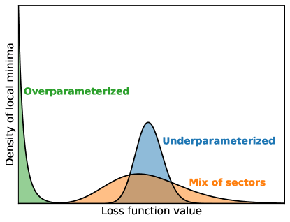
Figure 2: Density of local minima in various parameter regimes. The density of local minima when the quantum neural network is underparameterized, overparameterized, and when some algebraic sectors are underparameterized and some are overparameterized (mix of sectors). In the latter case, convolutions between various algebraic sectors broaden the distribution, though the proportion of minima near the global minimum in energy still vanishes exponentially in the system size due to the exponential tails of the gamma distribution.

Finally, by examining the joint distribution of the Wishart process over multiple inputs we are able to extend previously known results from the existing QNTK literature. We have shown generally that QNNs are Wishart processes rather than Gaussian processes; thus, we can exactly characterize the special cases when these Wishart processes asymptotically converge to a Gaussian process. We show that convergence to the QNTK only occurs when higher-order cumulants of the Wishart process asymptotically vanish and a central-limit-like theorem holds.

Corollary 4 (Exact conditions for convergence to a Gaussian process, informal).

Consider a QNN with loss function $\ell$ and objective observable $\bm{O}$ in an $N$-dimensional Hilbert space. Let $\bm{O}$ have mean eigenvalue $\overline{o}$ and let

$$r=\frac{\Tr\left(\bm{O}\right)^{2}}{\Tr\left(\bm{O}^{2}\right)}.$$ (8)

The rescaled loss function $\mathcal{N}\ell$ of the QNN is a Gaussian process in the limit $N\to\infty$ if and only if:

1. $\mathcal{N}\leq\operatorname{O}\left(\sqrt{r}\right)$.

2. $\mathcal{N}^{2}\operatorname{Var}\left[\ell\left(\bm{\rho}\right)\right]$ has a well-defined, nonzero limit for all $\bm{\rho}$ in the data set, where $\operatorname{Var}\left[\ell\left(\bm{\rho}\right)\right]$ is as in Eq. (5).

When the QNN asymptotically converges to a Gaussian process we are also able to explicitly write the covariance $\mathcal{K}\left(\bm{\rho},\bm{\rho^{\prime}}\right)$ in terms of the algebraic properties of the network. In particular, we show that this covariance is some fixed quadratic functional in its arguments.

Theorem 5 ($\mathcal{K}$ is quadratic in $\bm{\rho},\bm{\rho^{\prime}}$).

$\mathcal{K}\left(\bm{\rho},\bm{\rho^{\prime}}\right)$ can be written as a closed-form, explicit function of only the $\Tr\left(\bm{\rho}^{\alpha}\right)$, $\Tr\left(\bm{\rho^{\prime}}^{\alpha}\right)$, $\Tr\left(\left(\bm{\rho}^{\alpha}\right)^{2}\right)$, $\Tr\left(\left(\bm{\rho^{\prime}}^{\alpha}\right)^{2}\right)$, and $\Tr\left(\bm{\rho}^{\alpha}\bm{\rho^{\prime}}^{\alpha}\right)$.

Due to the relatively simple nature of the covariance, we hope in the future to use the nice properties of Wishart processes to directly deduce generalizations of NTK-like properties for non-Gaussian QNN loss landscapes.

I.3 Discussion

Taken together, our results show that the natural model for quantum neural networks is not one of Gaussian processes obeying a quantum neural tangent kernel, but rather one of Wishart processes. This Wishart process model unifies all of the recent major thrusts in calculating properties of quantum neural network loss landscapes. Indeed, our results allow us to propose a simple definition for the “trainability” of quantum neural networks, which to date has been a term used heuristically without any formal definition.

Definition 6 (Trainability of quantum neural networks).

Consider a QNN in a Hilbert space of dimension $N$ with $p$ trained parameters. Let $\mathcal{A}\cong\bigoplus\limits_{\alpha}\mathcal{A}_{\alpha}$ be the corresponding Jordan algebra as previously described. Define the degrees of freedom parameter:

$$r_{\alpha}\equiv\frac{\Tr\left(\bm{O}^{\alpha}\right)^{2}}{\Tr\left(\left(\bm{O}^{\alpha}\right)^{2}\right)}.$$ (9)

We say that the QNN is trainable if and only if, as $N\to\infty$, the QNN satisfies:

1. Absence of barren plateaus (Corollary 2):

   $$\sum\limits_{\alpha}\frac{\Tr\left(\left(\bm{O}^{\alpha}\right)^{2}\right)\Tr\left(\left(\bm{\rho}^{\alpha}\right)^{2}\right)}{\dim_{\mathbb{R}}\left(\mathfrak{g}_{\alpha}\right)}=\operatorname{\Omega}\left(\operatorname{poly}\left(\log\left(N\right)\right)^{-1}\right).$$ (10)

2. Absence of poor local minima (Corollary 3):

   $$p\geq\max\limits_{\alpha}\beta_{\alpha}r_{\alpha}.$$ (11)

Practically, where does this leave quantum neural networks? For one, it seems unlikely that there exists any computational quantum advantage during the training of QNNs—outside of HHL-like speedups [25, 26]—that does not leverage some existing knowledge of the data to be learned as in Refs. [27, 28, 29]. This was noted in Ref. [19] for deep QNNs, where the authors postulated that deep QNNs exhibiting no barren plateaus are classically simulable (outside of certain special cases). This is due to the fact that barren plateaus exist in deep QNNs when the explored Hilbert space grows superpolynomially quickly with the system size, which is typically a prerequisite for demonstrating a superpolynomial quantum computational advantage. Our results demonstrate a similar phenomenon for shallow QNNs: poor local minima in polynomially-sized circuits can only be avoided when the effective Hilbert space dimension grows at most polynomially quickly with the system size. This leaves the space for a practical, superpolynomial quantum advantage when training with a problem-agnostic algorithm such as gradient descent even narrower than previously believed: a veritable Amity Island in a sea of negative results.

However, polynomial quantum advantages during inference—i.e., after training—are certainly still on the table. Indeed, Refs. [20, 21] have demonstrated this for certain translation problems. One interpretation of their demonstrated results is that they prove the existence—for any constant $k$—of “quantum-inspired classical” recurrent neural networks of size $N$ that, once trained on a classical computer, can be compiled to a quantum device on $N^{\frac{1}{k}}$ qumodes. This network only requires $\log\left(N\right)$-depth quantum circuits in each unit cell. They also demonstrate that there exist machine learning tasks with classical memory lower-bounds of $N$ that these networks can perform to zero error. We argue that this is the setting future research should be devoted to searching for practical quantum advantages in machine learning: learning scenarios where the quantum models are provably trainable, and achieve some sort of quantum advantage over classical networks during inference.

There are some interesting questions that our results pose. For one, we only study the local minima distribution in detail when the eigenvalue spectrum of the objective observable is concentrated as is typical of low-weight fermionic [30] and local spin Hamiltonians [31]. However, the behavior of the local minima density differs when the spectrum is not concentrated, as is typical of observables drawn from the Gaussian unitary ensemble (GUE) and nonlocal spin systems. Observables from this latter class are known to be “quantumly easy” in the sense that phase estimation performed on the maximally mixed state efficiently prepares the ground state [32]. Based on this intuition these nonlocal systems may also yield local minima distributions for quantum neural networks more amenable to variational optimization even at shallow depth. If this is true, this may give a natural class of optimization problems which are easy to solve given access to a quantum computer.

Furthermore, given the importance of noise in current-generation quantum hardware, it would be important to understand generalizations of this work to quantum channels. It is already known that noise can affect the presence of barren plateaus [33] as well as local minima [34, 35] in variational loss landscapes. Heuristically the former can be understood as an additional channel mixing the variational ansatz over Hilbert space, and the latter as noise effectively limiting the number of parameters influencing the variational ansatz and thus always keeping the network in the underparameterized regime. We hope in the future to make this heuristic understanding rigorous.

The exact density of local minima—in particular, if one has control of the second moment of the local minima density, which we do not study here—of classical spin glass systems is known to have intriguing connections not only to the true ground state value [36] but also to general (i.e., beyond gradient descent) algorithmic thresholds for optimizing spin glasses [37]. Studying second moments of quantum spin glass local minima distributions may thus be a tractable avenue for studying the algorithmic hardness of quantum problems, as well as avoiding the need to study generalizations of the Parisi formula to the quantum setting in order to evaluate the quenched free energy of quantum systems. This would have important implications beyond a variational optimization perspective.

Finally, our work gives a unified understanding of quantum neural networks as Wishart processes. Great strides have been made in the classical machine learning literature in understanding the training dynamics [2, 3, 5, 6] and generalization behavior [5, 7] of classical neural networks via their connections to Gaussian processes, which unfortunately only port over in the specific settings where the Wishart process itself approaches the QNTK [11, 12, 13]. Fully understanding how specific properties of the Wishart process influence the learning behavior of the network seems the most natural way forward for using random matrix theory to understand how quantum neural networks learn.

II Preliminaries

We begin by reviewing concepts that we will use in proving our results. We also give a summary of the notation we use throughout in Table 1.

$\mathbb{N}_{0}$	Natural numbers including $0$
$\mathbb{N}_{1}$	Natural numbers excluding $0$
$\left[n\right]$	Natural numbers from $1$ through $n$
$\mathcal{H}^{n}\left(\mathbb{F}\right)$	Jordan algebra of $n\times n$ Hermitian matrices over $\mathbb{F}$
$\mathbb{F}$	Field, here one of $\mathbb{R},\mathbb{C},\mathbb{H}$
$\beta$	$\beta=1,2,4$ when associated field $\mathbb{F}=\mathbb{R},\mathbb{C},\mathbb{H}$, respectively
$\dim_{\mathbb{F}}\left(\cdot\right)$	Dimension of $\cdot$ as a vector space over $\mathbb{F}$
$\mathcal{N}^{\beta}\left(0,1\right)$	Standard normal distribution over $\mathbb{F}$ (given by $\beta$)
$\mathcal{W}_{n}^{\beta}\left(r,\bm{\varSigma}\right)$	$\beta$-Wishart distribution of $n\times n$ matrices with $r$ degrees of freedom and scale matrix $\bm{\varSigma}$
$\rightsquigarrow$	Convergence in distribution
$\xrightarrow{p}$	Convergence in probability
$\odot$	Hadamard product
$\mathcal{A}_{\alpha}$	Simple components of semisimple Jordan algebra $\mathcal{A}$
$G_{\alpha}$	Lie group isomorphic to a connected component of $\operatorname{Aut}\left(\mathcal{A}_{\alpha}\right)$
$\mathfrak{g}_{\alpha}$	Lie algebra generating $G_{\alpha}$
$\cdot^{\alpha}$	Defining representation of the projection of $\cdot$ into $\mathcal{A}_{\alpha}$
$N_{\alpha}$	Dimension of vector space on which the defining representation of $\mathcal{A}$ acts
$N$	Sum of $N_{\alpha}$
$\Tr_{\alpha}\left(\cdot\right)$	Trace of $\cdot$ in the defining representation of $\mathcal{A}_{\alpha}$
$\Tr\left(\cdot\right)$	Trace of $\cdot$ according to its representation in $\mathcal{H}^{N}\left(\mathbb{C}\right)\supseteq\mathcal{A}$
$\left\lVert\cdot\right\rVert_{\text{op}}$	Operator norm of $\cdot\in\mathcal{A}_{\alpha}$ in its defining representation
$\left\lVert\cdot\right\rVert_{\ast}$	Trace (nuclear) norm of $\cdot\in\mathcal{A}_{\alpha}$ in its defining representation
$\left\lVert\cdot\right\rVert_{\textrm{F}}$	Frobenius norm of $\cdot\in\mathcal{A}_{\alpha}$ in its defining representation
$\operatorname{O}\left(\operatorname{poly}\left(N\right)\right)$	$\operatorname{O}\left(N^{\kappa}\right)$ for some constant $\kappa>0$
WLOG	without loss of generality
w.h.p.	with high probability

Table 1: Table of notation. Notation used in the presentation of our results are given in the left column with corresponding meaning given in the right column. We also note here that exponents written as decimals throughout our results are chosen somewhat arbitrarily, i.e., can be improved by any sufficiently small constant $\epsilon>0$ in the exponent. Finally, we note that we will often forgo writing “…a sequence of [ansatzes, loss functions, observables, QNNs, …]…” when describing our asymptotic convergence results for brevity.

II.1 Quantum Neural Networks

We first review quantum neural networks (QNNs). These are defined by a parameterized ansatz

$$\bm{U}\left(\bm{\theta}\right)=\prod\limits_{i=p}^{1}\exp\left(-\mathrm{i}\theta_{i}\bm{A}_{i}\right)$$ (12)

with the goal of minimizing an empirical risk of the form:

$$f\left(\bm{\theta};\bm{\rho}\right)=\frac{1}{\left\lvert\mathcal{R}\right\rvert}\sum\limits_{\bm{\rho}\in\mathcal{R}}\ell\left(\bm{\theta};\bm{\rho}\right)=\frac{1}{\left\lvert\mathcal{R}\right\rvert}\sum\limits_{\bm{\rho}\in\mathcal{R}}\Tr\left(\bm{U}\left(\bm{\theta}\right)\bm{\rho}\bm{U}\left(\bm{\theta}\right)^{\dagger}\bm{O}\right).$$ (13)

Here, $\mathcal{R}$ can be thought of a data set comprising multiple input states $\bm{\rho}$, and $\ell$ the loss function. Historically, when $\left\lvert\mathcal{R}\right\rvert=1$ QNNs have been referred to as variational quantum algorithms (VQAs) [8] due to their connection to finding variational approximations to the ground states of quantum Hamiltonians. There are known quantum-classical separations for the expressivity of quantum neural networks even when taking into account the requirement that the training procedure is efficient [27, 28, 29], though they require very specific training algorithms that take advantage of the structure of the data.

There has been recent hope that, with enough ansatz structure, efficient training may follow just via a simple application of gradient descent. This follows from the Lie algebra supported ansatz (LASA) literature, where it has been shown that if the generators $\mathrm{i}\bm{A}_{i}$ of the ansatz $\bm{U}$ as well as the (scaled) objective observable $\mathrm{i}\bm{O}$ belong to some Lie algebra $\mathfrak{g}$—called the dynamical Lie algebra [15]—gradients scale inversely with the dimension of $\mathfrak{g}$ [16, 17]. It is also conjectured that when $\dim\left(\mathfrak{g}\right)$ scales polynomially with the system size there exist polynomial-depth ansatzes that do not have poor local minima, which together with the large gradients would imply efficient trainability of these loss functions via gradient descent. Conditioned on this conjecture there have been results demonstrating expressivity separations in quantum machine learning where the QNN is efficiently trainable through a simple application of gradient descent [20, 21].

Though the LASA framework gives sufficient conditions for loss functions to have large gradients, it is known that they are not necessary. One example of this was demonstrated in Ref. [24], where it was shown that parameterized matchgate circuits with an objective observable given by constant-degree polynomials in Majorana fermions are efficiently trainable though they are not a part of the LASA setting. We claim that both settings are special cases of a Jordan algebraic understanding of variational loss functions. In preparation of discussing this connection we now review Jordan algebras.

II.2 Jordan Algebras

A Jordan algebra over the reals is formally a real vector space $V$ with a commutative multiplication operation $\circ$ acting on $u,v\in V$ satisfying the Jordan identity:

$$u\circ\left(\left(u\circ u\right)\circ v\right)=\left(u\circ u\right)\circ\left(u\circ v\right),$$ (14)

which ensures the associativity of the power. A simple example of a Jordan algebra over the reals is the real algebra $\mathcal{H}^{N}\left(\mathbb{C}\right)$ of $N\times N$ complex-valued Hermitian matrices with $\circ$ given by half the anticommutator. In particular, for any finite-dimensional quantum system both $\bm{O}$ and the inputs $\bm{\rho}$ in Eq. (13) belong to $\mathcal{H}^{N}\left(\mathbb{C}\right)$. We emphasize that though this algebra is typically written in terms of complex matrices it is still a real Jordan algebra. This is because, for instance, $\mathrm{i}\not\in\mathbb{R}$ multiplying a Hermitian matrix is no longer Hermitian. In fact, the Jordan algebra of Hermitian matrices is Euclidean (or formally real) as it satisfies the defining property [38]:

$$\forall A,B\in\mathcal{A},\,A\circ A+B\circ B=0\iff A=B=0.$$ (15)

It is apparent that all subalgebras of a formally real algebra are also formally real.

The real vector space $V$ with which a Jordan algebra is associated also has a natural linear transformation $L\left(u\right)$:

$$L\left(u\right)v\equiv u\circ v,$$ (16)

which can be viewed as the Jordan algebraic analogue of the adjoint representation of Lie algebras. This linear transformation gives rise to the canonical trace form:

$$\tau\left(u,v\right)\equiv\Tr\left(L\left(u\circ v\right)\right).$$ (17)

When $\tau$ is nonsingular we call the associated Jordan algebra $\mathcal{A}$ semisimple. As an example, for the algebra $\mathcal{H}^{N}\left(\mathbb{F}\right)$ of Hermitian matrices over the field $\mathbb{F}$, $\tau\left(u,v\right)$ is just the Frobenius inner product between $u$ and $v$. Just as is the case for semisimple Lie algebras, all symmetric bilinear forms on a semisimple Jordan algebra are identical up to an overall scaling. Specifically, for any symmetric bilinear form $\sigma$, there exists an element $z$ in the center of $\mathcal{A}$ such that (Theorem 10, Ref. [39]):

$$\sigma\left(u,v\right)=\tau\left(z\circ u,v\right).$$ (18)

For $\mathcal{A}=\mathcal{H}^{N}\left(\mathbb{C}\right)$ in the defining representation the center is just real multiples of the identity matrix, i.e., there exists a real $I\geq 0$ such that:

$$I\sigma\left(u,v\right)=\tau\left(u,v\right).$$ (19)

We call $I$ the index of $\sigma$ in analogy with Ref. [16] for Lie algebras.

Though perhaps not as famous as the classification of compact Lie groups, the semisimple Euclidean Jordan algebras have also been classified.

Theorem 7 (Classification of semisimple Euclidean Jordan algebras [23]).

Any semisimple Euclidean Jordan algebra is isomorphic to a direct sum of the simple Euclidean Jordan algebras:

• $\mathcal{L}_{N}$ for $N\geq 1$: the spin factor, with vector space equal to $\mathbb{R}^{N}$ and $\circ$ given by the operation

  $$\bm{x}\circ\bm{y}=\left(\bm{x}\cdot\bm{y},x_{1}\bm{\overline{y}}+y_{1}\bm{\overline{x}}\right),$$ (20)

  where $\overline{\cdot}$ denotes $\cdot$ with the first coordinate projected out;

• $\mathcal{H}^{N}\left(\mathbb{R}\right)$ for $N\geq 3$: $N\times N$ symmetric matrices over $\mathbb{R}$, with $\circ$ half the anticommutator;

• $\mathcal{H}^{N}\left(\mathbb{C}\right)$ for $N\geq 3$: $N\times N$ Hermitian matrices over $\mathbb{C}$, with $\circ$ half the anticommutator;

• $\mathcal{H}^{N}\left(\mathbb{H}\right)$ for $N\geq 3$: $N\times N$ Hermitian matrices over $\mathbb{H}$, with $\circ$ half the anticommutator;

• $\mathcal{H}^{3}\left(\mathbb{O}\right)$ for $N\geq 3$: $3\times 3$ Hermitian matrices over $\mathbb{O}$, with $\circ$ half the anticommutator.

We use the term defining representation to speak of the described matrix representations of these algebras. As the Hermitian octonion case is not an infinite family it is often called exceptional. We here are interested in asymptotic sequences of Jordan algebras so we will not be considering the exceptional case.

Every Jordan algebra $\mathcal{A}$ has associated with it an automorphism group $\operatorname{Aut}\left(\mathcal{A}\right)$. As an example, for $\mathcal{H}^{N}\left(\mathbb{R}\right)$ in the defining representation this is just given by the action of conjugation (under the usual matrix multiplication) by orthogonal matrices. More generally, the nonexceptional simple cases have automorphism groups [40]:

• $\operatorname{Aut}\left(\mathcal{L}_{N}\right)$: left-action of $\left\{1\right\}\times\operatorname{O}\left(N-1\right)$;

• $\operatorname{Aut}\left(\mathcal{H}^{N}\left(\mathbb{R}\right)\right)$: conjugation action of $\operatorname{PO}\left(N\right)$;

• $\operatorname{Aut}\left(\mathcal{H}^{N}\left(\mathbb{C}\right)\right)$: disjoint union of the conjugation action of $\operatorname{PU}\left(N\right)$, and the transpose followed by the conjugation action of $\operatorname{PU}\left(N\right)$;

• $\operatorname{Aut}\left(\mathcal{H}^{N}\left(\mathbb{H}\right)\right)$: conjugation action of $\operatorname{PSp}\left(N\right)$.

We are here primarily interested in the connected component $\operatorname{Aut}_{1}\left(\cdot\right)\subseteq\operatorname{Aut}\left(\cdot\right)$ containing the identity transformation, so we will only concern ourselves with the path-connected automorphism subgroups:

• $\operatorname{SO}\left(N-1\right)\cong\operatorname{Aut}_{1}\left(\mathcal{L}_{N}\right)\subset\operatorname{Aut}\left(\mathcal{L}_{N}\right)$;

• $\operatorname{SO}\left(N\right)\cong\operatorname{Aut}_{1}\left(\mathcal{H}^{N}\left(\mathbb{R}\right)\right)\subseteq\operatorname{Aut}\left(\mathcal{H}^{N}\left(\mathbb{R}\right)\right)$;

• $\operatorname{SU}\left(N\right)\cong\operatorname{Aut}_{1}\left(\mathcal{H}^{N}\left(\mathbb{C}\right)\right)\subset\operatorname{Aut}\left(\mathcal{H}^{N}\left(\mathbb{C}\right)\right)$;

• $\operatorname{Sp}\left(N\right)\cong\operatorname{Aut}_{1}\left(\mathcal{H}^{N}\left(\mathbb{H}\right)\right)\subset\operatorname{Aut}\left(\mathcal{H}^{N}\left(\mathbb{H}\right)\right)$.

Surprisingly, the automorphism groups of semisimple Jordan algebras are also classified. Given a decomposition of a semisimple Euclidean Jordan algebra $\mathcal{A}$ into simple components:

$$\mathcal{A}\cong\bigoplus\limits_{\alpha}\mathcal{A}_{\alpha},$$ (21)

the connected component of $\operatorname{Aut}_{1}\left(\mathcal{A}\right)\subseteq\operatorname{Aut}\left(\mathcal{A}\right)$ containing the identity is isomorphic to the direct product (Theorem 10, Ref. [22]):

$$\operatorname{Aut}_{1}\left(\mathcal{A}\right)\cong\bigtimes\limits_{\alpha}\operatorname{Aut}_{1}\left(\mathcal{A}_{\alpha}\right).$$ (22)

II.3 $\epsilon$-Approximate $t$-Designs Over $\operatorname{Aut}_{1}\left(\mathcal{A}\right)$

In order to discuss the structure of the loss function in any detail we will need to consider some choice of randomness over loss functions. To achieve this we will use $\epsilon$-approximate $t$-designs over $\operatorname{Aut}_{1}\left(\mathcal{A}\right)$. Our use of these designs formalizes the notion of approximate “independence” or “uniform initialization” of the ansatz with respect to the eigenbasis of a given objective observable, as when $\epsilon\to 0$ and $t\to\infty$ the ansatz is chosen in a completely group-invariant way over $\operatorname{Aut}_{1}\left(\mathcal{A}\right)$. By Eq. (22) these designs are (up to isomorphism) direct products of $\epsilon$-approximate $t$-designs over $\operatorname{SO}\left(N\right)$, $\operatorname{SU}\left(N\right)$, and $\operatorname{Sp}\left(N\right)$.

Before defining $\epsilon$-approximate $t$-designs we define the Haar measure on compact Lie groups such as $\operatorname{Aut}_{1}\left(\mathcal{A}\right)$. This is the unique group-invariant normalized measure on these compact Lie groups.

Definition 8 (Haar measure on $G$ [41]).

Let $G$ be a compact Lie group. The unique measure satisfying:

$$\int_{G}\differential{\mu}=1$$ (23)

as well as

$$\differential{\mu}=\differential{\left(g\mu\right)}$$ (24)

for all $g\in G$ is the Haar measure on $G$. The existence and uniqueness of this measure follows from Ref. [41].

We now define $\epsilon$-approximate $t$-designs. We will here use the “trace norm definition” out of convenience, though all of the commonly used definitions are roughly equivalent [42].

Definition 9 ($\epsilon$-approximate $t$-designs over $G$).

Let $G$ be a compact Lie group with defining representation over an $N$-dimensional space, and $\mu$ the Haar measure over $G$. A measure $\nu$ satisfying:

$$\sum\limits_{m}\left\lvert\mathbb{E}_{U\sim\mu}\left[m\left(U\right)\right]-\mathbb{E}_{U\sim\nu}\left[m\left(U\right)\right]\right\rvert\leq\epsilon,$$ (25)

where the sum is over all degree-$\left(t,t\right)$ monomials $m\left(U\right)$ in the entries of $U$ and $U^{\ast}$, is an $\epsilon$-approximate $t$-design over $G$.

II.4 Wishart Matrices

Our main results will be given in terms of Wishart-distributed random matrices, so before proceeding we give a brief review of this distribution. We will use $\mathcal{W}_{n}^{\beta}\left(r,\bm{\Sigma}\right)$ to denote the $\beta$-Wishart distribution [43], where:

• $\beta=1,2,4$ indicates it is over a field $\mathbb{R},\mathbb{C},\mathbb{H}$, respectively;

• $r\in\mathbb{N}_{1}$ is the degrees of freedom parameter of the distribution;

• $\bm{\varSigma}\in\mathcal{H}^{n}\left(\mathbb{R}\right)$ is the symmetric, real-valued, positive-definite scale matrix parameter of the distribution.

When we do not specify $\beta$ we implicitly are referring to the usual Wishart distribution where $\beta=1$. The $\beta$-Wishart distribution is over positive semidefinite matrices of rank $r$, constructed by drawing i.i.d. standard Gaussian entries over $\mathbb{F}$:

$$X_{i,j}\sim\mathcal{N}^{\beta}\left(0,1\right)$$ (26)

for $i\in\left[n\right]$ and $j\in\left[r\right]$, and considering the distribution of:

$$\bm{W}=\sqrt{\bm{\varSigma}}\bm{X}\bm{X}^{\dagger}\sqrt{\bm{\varSigma}}.$$ (27)

Here there exists the so-called Bartlett decomposition for $\bm{W}\sim\mathcal{W}_{n}^{\beta}\left(r,\bm{I}_{n}\right)$:

$$\bm{W}\sim\sqrt{\bm{\varSigma}}\bm{L}\bm{L}^{\dagger}\sqrt{\bm{\varSigma}},$$ (28)

where $\bm{L}$ is lower-triangular. When $r\geq n$, the the entries below the diagonal of $\bm{L}$ are i.i.d. $\mathcal{N}^{\beta}\left(0,1\right)$-distributed and the diagonal entries are i.i.d. distributed as [44]:

$$\beta L_{i,i}^{2}\sim\chi^{2}\left(\beta\left(r-i+1\right)\right),$$ (29)

i.e., the $L_{i,i}$ are $\chi$-distributed up to an overall scaling of $\beta^{-\frac{1}{2}}$. When $r<n$, $\bm{L}$ is $n\times r$ with first $r$ rows as above and all other entries i.i.d. according to $\mathcal{N}^{\beta}\left(0,1\right)$ [45, 46, 47]. This completely characterizes the marginal distribution of the entries of any $\bm{W}\sim\mathcal{W}_{n}^{\beta}\left(r,\bm{I}_{n}\right)$.

Our final results will be written in terms of real Wishart matrices $\bm{W}$, i.e., those with $\beta=1$. When we analyze the asymptotic density of local minima of a JAWS it will turn out we will need to consider the asymptotic spectrum of a real Wishart matrix, which we now discuss. When the scale matrix $\bm{\varSigma}$ of $\bm{W}$ is the identity, as $n,r\to\infty$ with $\frac{n}{r}=\gamma$ held constant, the spectrum of $r^{-1}\bm{W}$ is known to almost surely converge weakly to a fixed distribution [48]. This fixed distribution is the Marčenko–Pastur distribution, given by

$$\derivative{\mu_{\text{MP}}}{\lambda}=\left(1-\gamma^{-1}\right)\delta\left(\lambda\right)\bm{1}\left\{\gamma\geq 1\right\}+\frac{\sqrt{\left(\gamma_{+}-\lambda\right)\left(\lambda-\gamma_{-}\right)}}{2\uppi\gamma\lambda}\bm{1}\left\{\gamma_{-}\leq\lambda\leq\gamma_{+}\right\},$$ (30)

where

$$\gamma_{\pm}\equiv\left(1\pm\sqrt{\gamma}\right)^{2}$$ (31)

and $\bm{1}$ is the indicator function. This distribution is illustrated in Fig. 3.

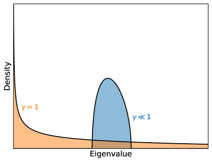
Figure 3: Marčenko–Pastur distribution. The density of the Marčenko–Pastur distribution—the asymptotic empirical eigenvalue distribution of normalized Wishart matrices—in the regime where $\gamma\ll 1$ and where $\gamma=1$. At $\gamma=1$ the associated Wishart matrix transitions from being full-rank to being low-rank.

II.5 Convergence of Random Variables

We finally discuss in more detail the various of notions of convergence of random variables that we use throughout our paper. Given a sequence of a set $\left(X_{i}^{N}\right)_{i}$ of real-valued random variables as $N\to\infty$, we say $\left(X_{i}^{N}\right)_{i}$ weakly converges (or converges in distribution) to $\left(X_{i}^{\infty}\right)_{i}$ if the joint cumulative distribution function $F^{N}$ of the $X_{i}^{N}$ converges to the joint cumulative distribution function $F^{\infty}$ of the $X_{i}^{\infty}$ at every point at which $F^{\infty}$ is continuous. That is,

$$\lim\limits_{N\to\infty}F^{N}\left(\bm{x}\right)=F^{\infty}\left(\bm{x}\right)$$ (32)

for all points $\bm{x}$ at which $F^{\infty}$ is continuous. We denote this at the level of random variables with the notation:

$$\left(X_{i}^{N}\right)_{i}\rightsquigarrow\left(X_{i}^{\infty}\right)_{i}.$$ (33)

One way to quantify the rate of this convergence is through the use of the Lévy–Prokhorov metric. Letting $p^{N}$ and $p^{\infty}$ be the densities associated with $F^{N}$ and $F^{\infty}$, respectively, the Lévy–Prokhorov metric is given by:

$$\pi\left(p^{N},p^{\infty}\right)=\inf\left\{\epsilon>0\mid\forall A,\,F^{N}\left(A\right)\leq F^{\infty}\left(A^{\epsilon}\right)+\epsilon\right\},$$ (34)

where here $A^{\epsilon}$ is an $\epsilon$-neighborhood in $\infty$-norm of $A$. $\pi\left(p^{N},p^{\infty}\right)\to 0$ if and only if $\left(X_{i}^{N}\right)_{i}\rightsquigarrow\left(X_{i}^{\infty}\right)_{i}$.

Convergence in distribution is closely related to the pointwise convergence of probability densities. Indeed, the latter implies the former by Scheffé’s theorem [49]. The former implies the latter if the $p^{N}$ are equicontinuous and uniformly bounded as $N\to\infty$ [50].

We finally discuss convergence in probability. This is the statement that, for all $\epsilon>0$,

$$\lim\limits_{N\to\infty}\mathbb{P}\left(\left\lVert\bm{X}^{N}-\bm{X}^{\infty}\right\rVert_{\infty}>\epsilon\right)=0.$$ (35)

We denote this convergence using the notation:

$$\left(X_{i}^{N}\right)_{i}\xrightarrow{p}\left(X_{i}^{\infty}\right)_{i}.$$ (36)

One way to quantify convergence in probability is through the Ky Fan metric, which is given by:

$$\alpha\left(p^{N},p^{\infty}\right)=\inf\left\{\epsilon>0\mid\mathbb{P}\left(\left\lVert\bm{X}^{N}-\bm{X}^{\infty}\right\rVert_{\infty}>\epsilon\right)\leq\epsilon\right\}.$$ (37)

$\alpha\left(p^{N},p^{\infty}\right)\to 0$ if and only if $\left(X_{i}^{N}\right)_{i}\xrightarrow{p}\left(X_{i}^{\infty}\right)_{i}$. The Ky Fan metric upper bounds the Lévy–Prokhorov metric [51], consistent with the notion of convergence in probability implying convergence in distribution.

We will in what follows often be loose with language and say two sequences of distributions converge to one another at a rate $K$, either weakly or in probability, rather than state convergence to a fixed distribution. This should be understood to mean that their distance in associated metric asymptotically vanishes as $K^{-1}$.

III Main Results

III.1 The Jordan Algebraic Structure of Variational Loss Landscapes

With these preliminaries in place we can write the variational loss function given in Eq. (13) as the canonical trace form on $\mathcal{H}^{N}\left(\mathbb{C}\right)$:

$$\ell\left(\bm{\theta};\bm{\rho}\right)=\tau\left(\bm{\rho},T\left(\bm{\theta}\right)\bm{O}\right),$$ (38)

where here $\bm{\rho}\in\mathcal{H}^{N}\left(\mathbb{C}\right)$, $\bm{O}$ is a member of some semisimple Euclidean Jordan subalgebra $\mathcal{A}\subseteq\mathcal{H}^{N}\left(\mathbb{C}\right)$, and $T\left(\bm{\theta}\right)$ parameterizes some path-connected space

$$\mathcal{T}\subseteq\operatorname{Aut}\left(\mathcal{A}\right)\subseteq\operatorname{Aut}\left(\mathcal{H}^{N}\left(\mathbb{C}\right)\right).$$ (39)

We also assume WLOG that $\mathcal{T}$ includes the identity; if it does not, we redefine $\bm{O}\to T\left(\bm{0}\right)\bm{O}$ and $T\left(\bm{\theta}\right)\to T\left(\bm{\theta}\right)T\left(\bm{0}\right)^{-1}$. Because of this, we can instead consider:

$$\mathcal{T}\subseteq\operatorname{Aut}_{1}\left(\mathcal{A}\right).$$ (40)

As the trace form is zero for components of $\bm{\rho}$ orthogonal to $\mathcal{A}$ it is easy to see that we only need consider the projection of $\bm{\rho}$ onto $\mathcal{A}$. Because of this we will often consider $\bm{\rho}$ an element of $\mathcal{A}$ in a slight abuse of notation. We call a variational loss function of this form a Jordan algebra-supported ansatz (JASA), in analogy with the term Lie-algebra supported ansatz (LASA) introduced in Ref. [16]. However, whereas variational loss functions are LASAs only if $\mathrm{i}\bm{O}$ belongs to the dynamical Lie algebra generating the ansatz, all variational loss functions are JASAs (up to assuming the path-connectedness of $\mathcal{T}$). Indeed, in Appendix B we give a direct mapping from both LASAs and the variational matchgate formalism of Ref. [24] to JASAs and show that a mapping in the other direction is generally not possible.

We are often interested in the case where our variational loss landscape has some sort of structure. In the context of LASAs this structure was endowed by the Lie algebra to which the generators of the variational ansatz were constrained. Because of this, generic properties of the loss landscape could be deduced just by the structure of the dynamical Lie algebra, which fell into just one of a few cases due to the widely celebrated classification of compact Lie groups. For JASAs the equivalent structure is given by the semisimple Euclidean Jordan subalgebra $\mathcal{A}$ to which $\bm{O}$ belongs, which generally has a decomposition into simple sectors:

$$\mathcal{A}\cong\bigoplus\limits_{\alpha}\mathcal{A}_{\alpha},$$ (41)

where the $\mathcal{A}_{\alpha}$ are one of the (assumed nonexceptional) cases given in Theorem 7. We define:

$$N_{\alpha}\equiv\dim\left(\mathcal{A}_{\alpha}\right).$$ (42)

We use $\Tr_{\alpha}\left(\cdot\right)$ to denote the trace of $\cdot$ in the defining representation of $\mathcal{A}_{\alpha}$ and $\Tr\left(\cdot\right)$ to denote the trace of $\cdot$ according to its representation in $\mathcal{H}^{N}\left(\mathbb{C}\right)\supseteq\mathcal{A}$. In Appendix A we demonstrate that in the context of examining variational loss landscapes, the spin factor sectors ($\mathcal{A}_{\alpha}=\mathcal{L}_{N_{\alpha}}$) effectively reduce to real symmetric ($\mathcal{A}_{\alpha}=\mathcal{H}^{N_{\alpha}}\left(\mathbb{R}\right)$) sectors. Because of this, we will from here on out focus on the case when $\mathcal{A}_{\alpha}$ is the Jordan algebra of Hermitian matrices over a field, i.e., $\mathcal{A}_{\alpha}\cong\mathcal{H}^{N_{\alpha}}\left(\mathbb{F}_{\alpha}\right)$ for $\mathbb{F}_{\alpha}=\mathbb{R},\mathbb{C},\mathbb{H}$. We will also throughout use $\beta_{\alpha}=1,2,4$ to label these three cases, respectively, as is commonly done in the physics literature.

Recalling the universality of the trace form and the direct product decomposition of $\operatorname{Aut}\left(\mathcal{A}\right)$, we can rewrite the loss function of Eq. (38) as:

$$\ell\left(\bm{\theta};\bm{\rho}\right)=\sum\limits_{\alpha}\ell^{\alpha}\left(\bm{\theta};\bm{\rho}\right)\equiv\sum\limits_{\alpha}I_{\alpha}\tau^{\alpha}\left(\bm{\rho}^{\alpha},T^{\alpha}\left(\bm{\theta}\right)\bm{O}^{\alpha}\right),$$ (43)

where here $\cdot^{\alpha}$ is used to denote the component of $\cdot$ in $\mathcal{A}_{\alpha}$, $\tau^{\alpha}$ is the canonical trace form on $\mathcal{A}_{\alpha}$, and $I_{\alpha}>0$ is the constant due to Eq. (19).

We now give an explicit form for $T^{\alpha}\left(\bm{\theta}\right)$. Recall that elements of $\operatorname{Aut}_{1}\left(\mathcal{A}_{\alpha}\right)$ are, in the defining representation of $\mathcal{A}_{\alpha}$, given by the conjugation action by elements of $\operatorname{SO}\left(N_{\alpha}\right)$, $\operatorname{SU}\left(N_{\alpha}\right)$, or $\operatorname{Sp}\left(N_{\alpha}\right)$ when $\mathbb{F}_{\alpha}=\mathbb{R},\mathbb{C},\mathbb{H}$, respectively. We let $G_{\alpha}$ denote the corresponding Lie group and $\mathfrak{g}_{\alpha}$ the associated Lie algebra. We also denote $G$ as the direct product over $G_{\alpha}$, and $\mathfrak{g}$ the corresponding Lie algebra. Following the typical structure of variational quantum algorithms [8] we will assume $T^{\alpha}\left(\bm{\theta}\right)$ in the defining representation corresponds to conjugation by:

$$U_{\bm{g},h}^{\alpha}\left(\bm{\theta}\right)=g_{0}^{\alpha\dagger}\left(\prod\limits_{i=1}^{p}g_{i}^{\alpha}\exp\left(\theta_{i}A_{i}^{\alpha}\right)g_{i}^{\alpha\dagger}\right)h^{\alpha}\in G_{\alpha}$$ (44)

for some $g_{i},h\in G$ and $A_{i}\in\mathfrak{g}$, where $\cdot^{\alpha}$ denotes the projection onto $G_{\alpha}$ or $\mathfrak{g}_{\alpha}$ appropriately. With this choice of ansatz it is also easy to see the derivatives of $\ell$ have algebraic interpretations. For instance, at $\bm{\theta}=\bm{0}$, $i\geq j$,

$$\partial_{i}\ell\left(\bm{\theta};\bm{\rho}\right) =\sum\limits_{\alpha}I_{\alpha}\tau^{\alpha}\left(g_{0}^{\alpha}\bm{\rho}^{\alpha}g_{0}^{\alpha\dagger},\left[g_{i}^{\alpha}A_{i}^{\alpha}g_{i}^{\alpha\dagger},h^{\alpha}\bm{O}^{\alpha}h^{\alpha\dagger}\right]\right),$$ (45)

$$\partial_{i}\partial_{j}\ell\left(\bm{\theta};\bm{\rho}\right) =\sum\limits_{\alpha}I_{\alpha}\tau^{\alpha}\left(g_{0}^{\alpha}\bm{\rho}^{\alpha}g_{0}^{\alpha\dagger},\left[g_{j}^{\alpha}A_{j}^{\alpha}g_{j}^{\alpha\dagger},\left[g_{i}^{\alpha}A_{i}^{\alpha}g_{i}^{\alpha\dagger},h^{\alpha}\bm{O}^{\alpha}h^{\alpha\dagger}\right]\right]\right),$$ (46)

where the commutator action of the automorphism group of a Jordan algebra is canonically defined through its representation $L$ defined in Eq. (16) (see Lemma 7 of Ref. [22]).

III.2 Jordan Algebraic Wishart Systems

We have demonstrated that all variational loss landscapes are Jordan algebra-supported ansatzes (JASAs). We are finally ready to discuss our main results, which give an explicit expression for the loss landscape of a JASA when its ansatz takes the form of Eq. (44). To do this we first define a Jordan algebraic Wishart system (JAWS), leaving for now ambiguous the connection to Wishart matrices.

Definition 10 (Jordan algebraic Wishart system).

Let $O$ belong to a Jordan algebra $\mathcal{A}\subseteq\mathcal{H}^{N}\left(\mathbb{C}\right)$ and let $\mathcal{T}$ be a path-connected subspace $\mathcal{T}\subseteq\operatorname{Aut}_{1}\left(\mathcal{A}\right)$. Let

$$\mathcal{A}\cong\bigoplus\limits_{\alpha}\mathcal{A}_{\alpha}$$ (47)

be the decomposition of $\mathcal{A}$ into simple Euclidean components as in Theorem 7 with associated decomposition $\mathcal{T}\cong\bigoplus\mathcal{T}_{\alpha}$ as in Eq. (22). Let $\mathcal{G}_{i}^{\alpha},\mathcal{H}^{\alpha}$ be independent distributions over $\mathcal{T}_{\alpha}$, and $\bm{A}=\left\{A_{i}\right\}_{i=1}^{p}$ elements of the Lie algebra of $\operatorname{Aut}_{1}\left(\mathcal{A}\right)$. We call

$$\mathcal{J}=\left(\mathcal{A},\mathcal{T},\bm{\mathcal{G}},\bm{\mathcal{H}},\bm{A},O\right)$$ (48)

a Jordan algebraic Wishart system (JAWS).

Every JAWS has associated with it a loss function as discussed in Sec. III.1. Using $\cdot^{\alpha}$ to label the projection of $\cdot$ into $\mathcal{A}_{\alpha}$ in its defining representation, the associated loss function takes the form:

$$\ell\left(\bm{\theta};\bm{\rho}\right)=\sum\limits_{\alpha}\ell^{\alpha}\left(\bm{\theta};\bm{\rho}\right)=\sum\limits_{\alpha}I_{\alpha}\Tr_{\alpha}\left(\bm{\rho}^{\alpha}\bm{U}^{\alpha}\left(\bm{\theta}\right)\bm{O}^{\alpha}\bm{U}^{\alpha}\left(\bm{\theta}\right)^{\dagger}\right),$$ (49)

where $\bm{U}^{\alpha}\left(\bm{\theta}\right)\in G_{\alpha}$ for all $\bm{\theta}$ and is of the form:

$$\bm{U}^{\alpha}\left(\bm{\theta}\right)\equiv g_{0}^{\alpha\dagger}\left(\prod\limits_{i=1}^{p}g_{i}^{\alpha}\exp\left(\theta_{i}A_{i}^{\alpha}\right)g_{i}^{\alpha\dagger}\right)h^{\alpha}.$$ (50)

Here, $g_{i}^{\alpha}$ is the defining representation of an element drawn from from the distribution $\mathcal{G}_{i}^{\alpha}$, and $h^{\alpha}$ is similar for $\mathcal{H}^{\alpha}$.

Our main result is a concise, asymptotic description of $\ell\left(\bm{\theta};\bm{\rho}\right)$ when the ansatz is chosen “sufficiently independently” from $\bm{O}$ (up to respecting the algebra $\mathcal{A}$). More formally, the rate at which $\ell\left(\bm{\theta};\bm{\rho}\right)$ converges to its asymptotic limit depends on the parameters defined by the following assumption.

Assumption 11 ($\epsilon$-approximate $t$-design of observable basis).

Each $\mathcal{H}^{\alpha}$ is an $\epsilon$-approximate $t$-design over $\operatorname{Aut}_{1}\left(\mathcal{A}_{\alpha}\right)$.

If there is a sense of geometric locality in the system, i.e., if the reverse lightcone of $\bm{O}^{\alpha}$ is of the form:

$$\bm{U}^{\alpha}\left(\bm{\theta}\right)\bm{O}^{\alpha}\bm{U}^{\alpha}\left(\bm{\theta}\right)^{\dagger}=\bm{\tilde{O}}^{\alpha}\otimes\bm{I}$$ (51)

for some $\bm{\tilde{O}}^{\alpha}$ acting on a space of dimension at most $D\equiv\exp\left(\operatorname{O}\left(p^{d}\right)\right)$ for constant geometric dimension $d$, one can explicitly enforce this with only a modest overhead in circuit depth. Indeed, one may embed $\mathcal{A}_{\alpha}$ into qubits and use the construction of Ref. [42] to give a $d$-dimensional random circuit of depth $\operatorname{O}\left(\operatorname{poly}\left(t\right)p\right)$ that achieves this over $\operatorname{Aut}_{1}\left(\mathcal{H}^{2^{n}}\left(\mathbb{C}\right)\right)\supset\operatorname{Aut}_{1}\left(\mathcal{A}_{\alpha}\right)$ for some $n=\operatorname{O}\left(p^{d}\right)$ and $\epsilon=\exp\left(-\operatorname{\Omega}\left(p\right)\right)$.

Given Assumption 11 we are able to prove our main result on the convergence of loss functions. We are able to prove our convergence for any $N$-dependent overall normalization of the loss function $\mathcal{N}$, the only requirement being that central moments of sufficiently large (constant) order have a finite limit as $N\to\infty$. This is always true for $\mathcal{N}=1$ and, depending on the specific choice of $t$-design, potentially holds for any $\mathcal{N}\leq\operatorname{O}\left(N^{1-\delta}\right)$ where $\delta>0$ is constant.

Theorem 12 (Loss function distribution).

Let $\mathcal{J}$ be a JAWS satisfying Assumption 11 with loss function $\ell\left(\bm{\theta};\bm{\rho}\right)$ for $\bm{\rho}\in\mathcal{R}$. Further assume that

$$\Tr\left(\left(\bm{\rho}^{\alpha}\right)^{2}\right)=\operatorname{\Omega}\left(\frac{1}{N_{\alpha}^{0.999}}\right).$$ (52)

Fix $\bm{\theta}$. Assume $\mathcal{N}\leq\operatorname{O}\left(\min_{\alpha}N_{\alpha}^{0.99}\right)$ is such that there exists a constant $k^{\ast}$ such that the central moments of order $k>k^{\ast}$ of $\left(\mathcal{N}\ell\left(\bm{\theta};\bm{\rho}\right)\right)_{\bm{\rho}\in\mathcal{R}}$ are finite as all $\epsilon^{-1},t,N_{\alpha}\to\infty$. We have the convergence in joint distributions:

$$\left(\mathcal{N}\ell\left(\bm{\theta};\bm{\rho}\right)\right)_{\bm{\rho}\in\mathcal{R}}\rightsquigarrow\left(\mathcal{N}\hat{\ell}\left(\bm{\theta};\bm{\rho}\right)\right)_{\bm{\rho}\in\mathcal{R}}$$ (53)

as all $\epsilon^{-1},t,N_{\alpha}\to\infty$, where

$$\hat{\ell}\left(\bm{\theta};\bm{\rho}\right)\equiv\sum\limits_{\alpha}\hat{\ell}^{\alpha}\left(\bm{\theta};\bm{\rho}\right)\equiv\sum\limits_{\alpha}\frac{I_{\alpha}\overline{o}^{\alpha}}{r_{\alpha}}\Tr_{\alpha}\left(\bm{\rho}^{\alpha}\bm{W}^{\alpha}\right),$$ (54)

$\overline{o}^{\alpha}$ is the arithmetic mean eigenvalue of $\bm{O}^{\alpha}$ in the defining representation:

$$\overline{o}^{\alpha}=N_{\alpha}^{-1}\Tr_{\alpha}\left(\bm{O}^{\alpha}\right),$$ (55)

and the $\bm{W}^{\alpha}$ are independent Wishart-distributed random matrices with $\beta_{\alpha}r_{\alpha}$ degrees of freedom, where

$$r_{\alpha}\equiv\frac{\left\lVert\bm{O}^{\alpha}\right\rVert_{\ast}^{2}}{\left\lVert\bm{O}^{\alpha}\right\rVert_{\textrm{F}}^{2}}.$$ (56)

In particular, the distributions differ in Lévy–Prokhorov metric by

$$\pi=\operatorname{O}\left(\frac{\log\log\left(\mathcal{N}^{-t}\epsilon^{-1}\right)}{\log\left(\mathcal{N}^{-t}\epsilon^{-1}\right)}+\frac{\log\left(t\right)}{\sqrt{t}}+\sum\limits_{\alpha}\sqrt{\frac{\mathcal{N}\log\left(N_{\alpha}\right)}{N_{\alpha}^{1.001}}}\right)=\operatorname{o}\left(1\right).$$ (57)

In Appendix C we show that Eq. (52) can effectively be taken WLOG. This is because all $\bm{\rho}^{\alpha}$ for which this is not true are such that $\ell^{\alpha}\left(\bm{\theta};\bm{\rho}\right)$ have asymptotically vanishing variance even when rescaled by the potentially exponentially large $\mathcal{N}=\operatorname{O}\left(N\right)$. This is why we do not take Eq. (52) as a numbered Assumption. Examples of the loss density are illustrated in Fig. 4(a).

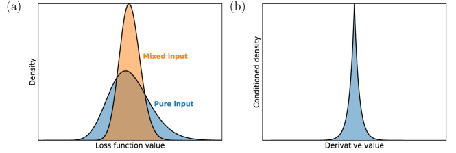
Figure 4: Loss and derivative densities. (a) A cartoon of the loss density when the quantum neural network has a pure input and when it has a mixed input. The distributions are centered at the mean eigenvalue of the objective observable. The mixed input density also illustrates the density when there are many algebraic sectors and any given input is mixed when projected into any one of them. (b) A cartoon of the gradient density conditioned on a nonzero loss function value. The distribution is centered at zero.

We can strengthen the statement of weak convergence in Theorem 12 to one of pointwise convergence of densities given equicontinuity and boundedness of the appropriately normalized loss function density. Whether this is true depends on the specifics of the distributions $\bm{\mathcal{G}},\bm{\mathcal{H}}$, particularly whether the loss is equicontinuous and bounded at the same $\mathcal{N}=\sqrt{r_{\alpha}}$ scale as $\hat{\ell}^{\alpha}$. We give some standard examples where this is true in Appendix E.

Corollary 13 (Convergence of loss function densities).

Let $\mathcal{J},\ell,\hat{\ell}$ be as in Theorem 12. Assume the density of $\left(\sqrt{r_{\alpha}}\ell^{\alpha}\left(\bm{\theta};\bm{\rho}\right)\right)_{\bm{\rho}\in\mathcal{R},\alpha}$ is equicontinuous and bounded as all $\epsilon^{-1},t,N_{\alpha}\to\infty$. Then the joint density of $\left(\sqrt{r_{\alpha}}\ell^{\alpha}\left(\bm{\theta};\bm{\rho}\right)\right)_{\bm{\rho}\in\mathcal{R},\alpha}$ is pointwise equal to that of $\left(\sqrt{r_{\alpha}}\hat{\ell}^{\alpha}\left(\bm{\theta};\bm{\rho}\right)\right)_{\bm{\rho}\in\mathcal{R},\alpha}$ up to an additive error $\operatorname{O}\left(\pi\right)$.

As-written our result only gives the loss function distribution at a single point $\bm{\theta}$ in parameter space. However, any finite set $\varTheta$ of points in parameter space can be considered by taking

$$\bm{\rho}\left(\bm{\theta}\right)=\bm{U}^{\alpha}\left(\bm{\theta}\right)\bm{\rho}\bm{U}^{\alpha\dagger}\left(\bm{\theta}\right)$$ (58)

to be elements in an augmented set of input states:

$$\mathcal{R}^{\prime}=\mathcal{R}\times\varTheta.$$ (59)

We can give a more concrete form for the parameter-dependence of the loss landscape by considering the joint distribution of $\ell$ with its derivatives. We begin with the gradient. In order to consider the joint distribution over what can potentially be many gradient components—a number growing with the number of parameters $p$—we take the following additional assumption on the growth of $t$ with $p$ so we are able to fully capture correlations between the derivatives.

Assumption 14 (Scaling of parameter space dimension with $t$-design).

The number of trained parameters $p$ satisfies:

$$p^{2}\leq\operatorname{o}\left(\min\left(\frac{\log\left(\epsilon^{-1}\right)}{\log\log\left(\epsilon^{-1}\right)},\frac{\sqrt{t}}{\log\left(t\right)}\right)\right),$$ (60)

where the $\mathcal{G}_{i}^{\alpha}$ are i.i.d. $\epsilon$-approximate $t$-designs over $\operatorname{Aut}_{1}\left(\mathcal{A}_{\alpha}\right)$, and

$$p\leq\operatorname{O}\left(\operatorname{poly}\left(\min\limits_{\alpha}N_{\alpha}\right)\right).$$ (61)

It is possible to weaken this assumption and instead assume that the $\mathcal{G}_{i}^{\alpha}$ are $\epsilon$-approximate $2$-designs rather than $t$-designs, but this is at the expense of requiring $\mathcal{N}\leq\operatorname{o}\left(N^{\frac{2}{3}}\right)$ and only considering jointly at most $\sim\log\left(N\right)$ components of the gradient. We leave further details of this alternative setting to Appendix D.

It will also be convenient for the rest of our discussion to consider a concrete set of $\bm{A}_{i}$.

Assumption 15 (Concrete choice of $\bm{A}_{i}$).

For $\mathbb{F}_{\alpha}=\mathbb{C},\mathbb{H}$, the $\bm{A}_{i}^{\alpha}$ are rank $1$. For $\mathbb{F}_{\alpha}=\mathbb{R}$, the $\bm{A}_{i}^{\alpha}$ are rank $2$.

The distinction between the cases $\mathbb{F}_{\alpha}=\mathbb{C},\mathbb{H}$ and $\mathbb{F}_{\alpha}=\mathbb{R}$ is due to there being no rank $1$ operators in the defining representation of $\mathfrak{so}\left(N_{\alpha}\right)$. This choice of $\bm{A}_{i}^{\alpha}$ may seem unphysical due to their nonlocality, but one can emulate the behavior of high-rank (e.g., Pauli) rotations by considering a factor of $N_{\alpha}$ more layers $p_{\alpha}$ in a given simple sector—each, for instance, performing a rotation under each eigenvector of $\bm{A}_{i}^{\alpha}$—and then tying the associated parameters together. This breaks no other assumptions as taking $p_{\alpha}\to N_{\alpha}p_{\alpha}$ maintains Eq. (61).

We then have the following theorem. It is stated assuming only a single input $\bm{\rho}$ which is rank-$1$ when projected to the defining representation of each simple sector to simplify the final result. However, in Sec. V.3 we give a full, exact expression of the joint distribution in terms of Wishart matrix elements for any choice of $\mathcal{R}\ni\bm{\rho}$ and independent of the scaling of $N_{\alpha}-r_{\alpha}$.

Theorem 16 (Gradient distribution).

Consider the setting of Theorem 12, with the additional Assumptions 14 and 15. Assume $\frac{\sigma_{o}^{\alpha}}{\overline{o}}$ is bounded—where $\sigma_{o}^{\alpha}$ is the standard deviation of the eigenvalues of $\bm{O}^{\alpha}$—and assume $\left\lvert\mathcal{R}\right\rvert=1$ with element $\bm{\rho}$ such that each $\bm{\rho}^{\alpha}$ is rank-$1$ in its defining representation. We have the convergence in joint distributions:

$$\left(\mathcal{N}\ell\left(\bm{\theta};\bm{\rho}\right),\mathcal{N}\partial_{i}\ell\left(\bm{\theta};\bm{\rho}\right)\right)_{i\in\left[p\right]}\rightsquigarrow\left(\mathcal{N}\hat{\ell}\left(\bm{\theta};\bm{\rho}\right),\mathcal{N}\hat{\ell}_{;i}\left(\bm{\theta};\bm{\rho}\right)\right)_{i\in\left[p\right]}$$ (62)

as all $\epsilon^{-1},t,N_{\alpha}\to\infty$, where conditioned on

$$\hat{\ell}^{\alpha}\left(\bm{\theta};\bm{\rho}\right)=z^{\alpha}$$ (63)

we have that

$$\hat{\ell}_{;i\mid z^{\alpha}}^{\alpha}\left(\bm{\theta};\bm{\rho}\right)=\frac{2I_{\alpha}\sigma_{o}^{\alpha}\Tr_{\alpha}\left(\bm{\rho}^{\alpha}\right)}{N_{\alpha}}\sqrt{\frac{\beta_{\alpha}z^{\alpha}}{I_{\alpha}\overline{o}^{\alpha}}}\chi_{i}^{\alpha}G_{i}^{\alpha},$$ (64)

where

$$\hat{\ell}_{;i}\left(\bm{\theta};\bm{\rho}\right)\mid\left\{\hat{\ell}^{\alpha}\left(\bm{\theta},\bm{\rho}\right)=z^{\alpha}\right\}_{\alpha}\equiv\hat{\ell}_{;i\mid\bm{z}}\left(\bm{\theta};\bm{\rho}\right)\equiv\sum\limits_{\alpha}\hat{\ell}_{;i\mid z^{\alpha}}^{\alpha}\left(\bm{\theta};\bm{\rho}\right).$$ (65)

Here, the $\chi_{i}^{\alpha}$ are independent $\chi$-distributed random variables with $\max\left(2,\beta_{\alpha}\right)$ degrees of freedom and the $G_{i}^{\alpha}$ are i.i.d. standard normal random variables. In particular, the distributions differ in Lévy–Prokhorov metric by

$$\pi^{\prime}=\operatorname{O}\left(\frac{p\log\log\left(\mathcal{N}^{-t}\epsilon^{-1}\right)}{\log\left(\mathcal{N}^{-t}\epsilon^{-1}\right)}+\frac{p\log\left(t\right)}{\sqrt{t}}+\sum\limits_{\alpha}\sqrt{\frac{\mathcal{N}\log\left(N_{\alpha}\right)}{N_{\alpha}^{1.001}}}+\frac{\mathcal{N}^{\frac{1}{3}}\log\left(N\right)}{N^{\frac{5}{12}}}\right)=\operatorname{o}\left(1\right).$$ (66)

This result is stronger than typical barren plateau results as it gives the full distributional form of the gradient—even when conditioned on the loss contribution $z^{\alpha}$—rather than just its variance [14, 15, 16, 17]. The conditional distribution as in Eq. (64) is illustrated in Fig. 4(b).

Just as with the loss function, we can strengthen Theorem 16 to show pointwise convergence in probability densities assuming equicontinuity of the original distribution.

Corollary 17 (Convergence of gradient densities).

Let $\mathcal{J},\ell,\hat{\ell}$ be as in Corollary 13. Assume the density of $\left(\sqrt{r_{\alpha}}\ell_{;i}^{\alpha}\left(\bm{\theta};\bm{\rho}\right)\right)_{\alpha}$ is equicontinuous and bounded for all $z^{\alpha}\in\mathbb{R}_{\geq 0}$ as all $\epsilon^{-1},t,N_{\alpha}\to\infty$. Then the joint density of $\left(\sqrt{r_{\alpha}}\ell_{;i}^{\alpha}\left(\bm{\theta};\bm{\rho}\right)\right)_{\alpha}$ is pointwise equal to that of $\left(\sqrt{r_{\alpha}}\hat{\ell}_{;i}^{\alpha}\left(\bm{\theta};\bm{\rho}\right)\right)_{\alpha}$ up to an additive error $\operatorname{O}\left(\pi^{\prime}\right)$.

We now give our final result, which specifies the joint distribution of not only the loss and gradient but also the Hessian at critical points. This is required to reason about the critical point distribution of the loss landscape using the so-called Kac–Rice formula [52] that we will discuss in detail in Sec. IV.3. We state our result assuming $\sigma_{o}\ll\overline{o}$ for simplicity, giving as we did for the gradient the full expression in terms of Wishart matrix elements in Sec. V.3.

Theorem 18 (Hessian distribution).

Let $\mathcal{J},\ell,\hat{\ell}$ be as in Theorem 16. Assume all $\frac{\sigma_{o}^{\alpha}}{\overline{o}^{\alpha}}=\operatorname{o}\left(1\right)$ as $N_{\alpha}\to\infty$. We have the convergence in joint distributions:

$$\left(\ell\left(\bm{\theta};\bm{\rho}\right),\partial_{i}\ell\left(\bm{\theta};\bm{\rho}\right),\partial_{i}\partial_{j}\ell\left(\bm{\theta};\bm{\rho}\right)\right)_{\bm{\rho}\in\mathcal{R},i,j\in\left[p\right]}\rightsquigarrow\left(\hat{\ell}\left(\bm{\theta};\bm{\rho}\right),\hat{\ell}_{;i}\left(\bm{\theta};\bm{\rho}\right),\hat{\ell}_{;i,j}\left(\bm{\theta};\bm{\rho}\right)\right)_{\bm{\rho}\in\mathcal{R},i,j\in\left[p\right]}$$ (67)

as all $\epsilon^{-1},t,N_{\alpha}\to\infty$, where conditioned on

$$\hat{\ell}^{\alpha}\left(\bm{\theta};\bm{\rho}\right)=z^{\alpha}$$ (68)

and

$$\hat{\ell}_{;i\mid z^{\alpha}}^{\alpha}\left(\bm{\theta};\bm{\rho}\right)=0$$ (69)

we have that

$$\hat{\ell}_{;i,j\mid z^{\alpha},0}^{\alpha}\left(\bm{\theta};\bm{\rho}\right)=\frac{2I_{\alpha}\sigma_{o}^{\alpha}\Tr_{\alpha}\left(\bm{\rho}^{\alpha}\right)}{N_{\alpha}^{2}}\sqrt{\frac{z^{\alpha}}{I_{\alpha}\overline{o}_{\alpha}}}G_{i}^{\alpha}\chi_{j}^{\alpha}\bra{i}\bm{W}^{\alpha}\ket{j},$$ (70)

where

$$\hat{\ell}_{;i,j}\left(\bm{\theta};\bm{\rho}\right)\mid\left\{\hat{\ell}^{\alpha}\left(\bm{\theta},\bm{\rho}\right)=z^{\alpha},\left(\hat{\ell}_{;i}^{\alpha}\left(\bm{\theta};\bm{\rho}\right)\right)_{i\in\left[p\right]}=\bm{0}\right\}_{\alpha}\equiv\hat{\ell}_{;i,j\mid\bm{z},\bm{0}}\left(\bm{\theta};\bm{\rho}\right)\equiv\sum\limits_{\alpha}\hat{\ell}_{;i,j\mid z^{\alpha},0}^{\alpha}\left(\bm{\theta};\bm{\rho}\right).$$ (71)

Here, the $G_{i}^{\alpha}$ are i.i.d. standard normal random variables, the $\chi_{i}^{\alpha}$ are independent $\chi$-distributed random variables with $\max\left(2,\beta_{\alpha}\right)$ degrees of freedom, and the $\bm{W}^{\alpha}$ are independent Wishart-distributed random matrices with $\beta_{\alpha}r_{\alpha}$ degrees of freedom. In particular, the distributions differ in Lévy–Prokhorov metric by

$$\pi^{\prime\prime}=\operatorname{O}\left(\frac{p^{2}\log\log\left(\mathcal{N}^{-t}\epsilon^{-1}\right)}{\log\left(\mathcal{N}^{-t}\epsilon^{-1}\right)}+\frac{p^{2}\log\left(t\right)}{\sqrt{t}}+\sum\limits_{\alpha}\frac{\mathcal{N}^{\frac{1}{3}}\log\left(N_{\alpha}\right)}{N_{\alpha}^{\frac{1}{3}}}\right)=\operatorname{o}\left(1\right).$$ (72)

IV Consequences of Our Results

Before proceeding with proofs of our results we examine their implications.

IV.1 Barren Plateaus

The first implication of our results that we will discuss is the unification of barren plateau results [16, 17] in the large $N_{\alpha}$ limit.

Corollary 19 (General expression for the loss function variance).

Let $\ell$ be as in Theorem 12. The variance is:

$$\operatorname{Var}\left[\ell\left(\bm{\theta};\bm{\rho}\right)\right]=\sum\limits_{\alpha}\frac{\Tr\left(\left(\bm{O}^{\alpha}\right)^{2}\right)\Tr\left(\left(\bm{\rho}^{\alpha}\right)^{2}\right)}{\dim_{\mathbb{R}}\left(\mathfrak{g}_{\alpha}\right)}+\operatorname{O}\left(\pi\right).$$ (73)

Here, $\dim_{\mathbb{R}}\left(\mathfrak{g}_{\alpha}\right)$ is the dimension of the automorphism group of $\mathcal{A}_{\alpha}$ and $\pi$ is as in Eq. (57).

Proof.

Note that

$$\dim_{\mathbb{R}}\left(\mathfrak{g}_{\alpha}\right)=\left(\beta_{\alpha}-1\right)N_{\alpha}+\frac{\beta_{\alpha}N_{\alpha}\left(N_{\alpha}-1\right)}{2}=\frac{\beta_{\alpha}N_{\alpha}^{2}}{2}+\operatorname{O}\left(N_{\alpha}\right).$$ (74)

Similarly,

$$\frac{\left(\overline{o}^{\alpha}\right)^{2}}{r_{\alpha}}=\frac{\left\lVert\bm{O}^{\alpha}\right\rVert_{\text{F}}^{2}}{N_{\alpha}^{2}}.$$ (75)

By Eq. (19), we also have that

$$I_{\alpha}\left\lVert\bm{O}^{\alpha}\right\rVert_{\text{F}}^{2}=\Tr\left(\left(\bm{O}^{\alpha}\right)^{2}\right),$$ (76)

with $\Tr\left(\cdot\right)$ the trace on the full $N$-dimensional Hilbert space. In the language of Ref. [17] this is the $\mathcal{A}_{\alpha}$-purity $\mathcal{P}_{\mathcal{A}_{\alpha}}$ of $\bm{O}$. Using the fact that the diagonal entries of $\beta_{\alpha}\bm{W}^{\alpha}$ are i.i.d. $\chi^{2}$-distributed with $\beta_{\alpha}r_{\alpha}$ degrees of freedom (see Sec. II.4), we then have from Theorem 12 that as $N_{\alpha}\to\infty$:

$$\operatorname{Var}\left[\ell\left(\bm{\theta};\bm{\rho}\right)\right] =\sum\limits_{\alpha}\operatorname{Var}\left[\hat{\ell}^{\alpha}\left(\bm{\theta};\bm{\rho}\right)\right]+\operatorname{O}\left(\pi\right)$$ (77)

$$=\sum\limits_{\alpha}\frac{2I_{\alpha}^{2}\left(\overline{o}^{\alpha}\right)^{2}}{\beta_{\alpha}r_{\alpha}}\Tr_{\alpha}\left(\left(\bm{\rho}^{\alpha}\right)^{2}\right)+\operatorname{O}\left(\pi\right)$$

$$=\sum\limits_{\alpha}\frac{2I_{\alpha}\left(\overline{o}^{\alpha}\right)^{2}}{\beta_{\alpha}r_{\alpha}}\Tr\left(\left(\bm{\rho}^{\alpha}\right)^{2}\right)+\operatorname{O}\left(\pi\right)$$

$$=\sum\limits_{\alpha}\frac{\Tr\left(\left(\bm{O}^{\alpha}\right)^{2}\right)\Tr\left(\left(\bm{\rho}^{\alpha}\right)^{2}\right)}{\dim_{\mathbb{R}}\left(\mathfrak{g}_{\alpha}\right)}+\operatorname{O}\left(\pi\right).$$

∎

This result immediately implies Theorem 1 of Ref. [17] in the case of Lie algebra supported ansatzes. However, our result holds for all variational ansatzes, i.e., it does not rely on either $\mathrm{i}\bm{O}$ or $\mathrm{i}\bm{\rho}$ being a member of the dynamical Lie algebra generating the ansatz.

IV.2 The Quantum Neural Tangent Kernel

We now connect our results to the quantum neural tangent kernel (QNTK) literature [11, 12, 13]. The landmark result in this field is that, under certain conditions on $\mathcal{R}$, $\bm{O}$, and $\mathcal{A}$, variational loss functions are asymptotically a Gaussian process when $\epsilon^{-1},t,N\to\infty$. However, this same body of work has noted that such a Gaussian process description cannot generally be true: for instance, if $\bm{O}$ is rank-$1$ and $\mathcal{A}$ is the space of complex Hermitian matrices, the loss should be Porter–Thomas distributed as this reduces to a random circuit sampling setting [53].

Our results can be seen as a unifying model of neural network loss landscapes, including both when convergence to a Gaussian process is achieved and when it is not. Recall that Theorem 12 demonstrated that the asymptotic expression for the variational loss with objective observable $\bm{O}$ is distributed as a Wishart process:

$$\hat{\ell}\left(\bm{\rho}\right)=\sum\limits_{\alpha}\frac{I_{\alpha}\overline{o}^{\alpha}}{r_{\alpha}}\Tr_{\alpha}\left(\bm{\rho}^{\alpha}\bm{W}^{\alpha}\right),$$ (78)

even when rescaled by a quantity $\mathcal{N}$ exponentially large in the problem size. This correctly captures the Porter–Thomas behavior when $\mathcal{A}$ is the space of complex Hermitian matrices and $\rank\left(\bm{O}\right)=r=1$. This is because the diagonal entries of a complex Wishart matrix are $\chi^{2}$-distributed with two degrees of freedom each, which is identical to the exponential distribution.

Indeed, our more general result can be used to exactly characterize when QNNs asymptotically form Gaussian processes. This occurs when the loss is scaled by some $\mathcal{N}$ such that Eq. (78) has nonvanishing variance yet the higher-order cumulants vanish. It is immediate from the distribution of Wishart matrix elements that the latter happens for any $\mathcal{N}\leq\operatorname{O}\left(\sqrt{r}\right)$. We thus can state this pair of conditions formally as follows.

Corollary 20 (Exact conditions for convergence to a Gaussian process).

Let $\mathcal{J},\ell$ be as in Theorem 12. $\mathcal{N}\ell\left(\bm{\theta};\bm{\rho}\right)$ is asymptotically a Gaussian process as $\epsilon^{-1},t,N\to\infty$ if and only if $\mathcal{N}\leq\operatorname{O}\left(\sqrt{r}\right)$ and the variance given in Corollary 19 is nonvanishing for all $\bm{\rho}\in\mathcal{R}$.

When these conditions are met, the covariance is given by:

$$\mathcal{K}\left(\bm{\rho},\bm{\rho^{\prime}}\right)=\lim\limits_{N\to\infty}\mathcal{K}_{N}\left(\bm{\rho},\bm{\rho^{\prime}}\right)=\lim\limits_{N\to\infty}\mathcal{N}^{2}\sum\limits_{\alpha}\frac{\Tr\left(\left(\bm{O}^{\alpha}\right)^{2}\right)}{r_{\alpha}^{2}}I_{\alpha}\mathbb{E}\left[\Tr_{\alpha}\left(\bm{\rho}^{\alpha}\left(\bm{W}^{\alpha}-r_{\alpha}\right)\right)\Tr_{\alpha}\left(\bm{\rho^{\prime}}^{\alpha}\left(\bm{W}^{\alpha}-r_{\alpha}\right)\right)\right].$$ (79)

It is now easy to see why (for simple $\mathcal{A}$) the $r=1$ case does not converge to a Gaussian process: when $r=1$ we may only choose a normalization $\mathcal{N}=\operatorname{O}\left(1\right)$, but here the variance vanishes asymptotically. In contrast, our results demonstrating convergence to a Wishart process hold for any $\mathcal{N}\leq\operatorname{O}\left(N^{1-\delta}\right)$ with $\delta>0$ fixed; in particular, any finite number of moments of a QNN can be shown to match that of a Wishart process, not just the first two.

We can also be more concrete on the form of $\mathcal{K}\left(\bm{\rho},\bm{\rho^{\prime}}\right)$. Indeed, we are able to show that each algebraic sector $\mathcal{A}_{\alpha}$ contributes to the covariance an explicit, quadratic expression in $\bm{\rho}^{\alpha}$ and $\bm{\rho^{\prime}}^{\alpha}$, depending only on the field $\mathbb{F}_{\alpha}$ associated with its defining representation. In other words, whether or not a given quantum neural network is asymptotically a Gaussian process just depends on how SWAP tests of the inputs scale. As the expression is complicated we do not reproduce it here, instead giving references to where it may be found for each of $\mathbb{F}_{\alpha}=\mathbb{R},\mathbb{C},\mathbb{H}$. See 5

Proof.

By the Haar invariance of $\bm{W}^{\alpha}$ there are explicit formulas for covariances of the form of $\mathcal{K}\left(\bm{\rho},\bm{\rho^{\prime}}\right)$ as degree-$2$ polynomials in $\bm{\rho}$ and $\bm{\rho^{\prime}}$. These formulas are given in:

1. Theorem 1 of Ref. [54] when $\mathbb{F}=\mathbb{R}$;

2. Theorem 3.5 of Ref. [55] when $\mathbb{F}=\mathbb{C}$;

3. Sec. 5.3 of Ref. [56] when $\mathbb{F}=\mathbb{H}$.

The result then follows by noting that $I_{\alpha}\Tr_{\alpha}\left(\cdot^{\alpha}\right)=\Tr\left(\cdot^{\alpha}\right)$. ∎

We give a simple example of the calculation of $\mathcal{K}$ when there is no algebraic structure and all inputs $\bm{\rho_{0}}$ can be mutually diagonalized. By the unitary invariance of Wishart matrices we can assume WLOG that all inputs are diagonal. Inputs are then completely parameterized by the eigenvalues $\bm{x}\in\mathbb{R}_{\geq 0}^{N_{\alpha}}$ of the input states, where $\left\lVert\bm{x}\right\rVert_{1}=1$. By the independence of diagonal entries of a Wishart matrix we then have that (when $\mathcal{N}=1$):

$$\mathcal{K}_{N}\left(\bm{x},\bm{x^{\prime}}\right) =\frac{\overline{o}^{2}}{r^{2}}\sum\limits_{i=1}^{N}x_{i}x_{i}^{\prime}\operatorname{Var}\left[\bra{i}\bm{W}\ket{i}\right]$$ (80)

$$=\frac{\overline{o}^{2}}{r}\bm{x}\cdot\bm{x}^{\prime}$$

$$=\frac{\Tr\left(\bm{O}^{2}\right)}{\dim_{\mathbb{R}}\left(\mathfrak{g}\right)}\bm{x}\cdot\bm{x}^{\prime}+\operatorname{o}\left(1\right),$$

where in the final line we used similar simplifications as in Sec. IV.1. Noting that $\bm{x}\cdot\bm{x}^{\prime}$ is just the overlap of $\bm{\rho}$ and $\bm{\rho^{\prime}}$ yields an equivalent formulation:

$$\mathcal{K}_{N}\left(\bm{\rho},\bm{\rho^{\prime}}\right)=\frac{\Tr\left(\bm{O}^{2}\right)}{\dim_{\mathbb{R}}\left(\mathfrak{g}\right)}\Tr\left(\bm{\rho}\bm{\rho^{\prime}}\right)+\operatorname{o}\left(1\right)=\operatorname{O}\left(\frac{1}{r}\right)\Tr\left(\bm{\rho}\bm{\rho^{\prime}}\right).$$ (81)

In particular, a $\mathcal{N}=\operatorname{\Theta}\left(\sqrt{r}\right)$ normalization is required for the network to asymptotically form a Gaussian process over pure inputs.

While previous results have shown that Gaussian processes efficiently train, we argue that this may paint an overly optimistic picture for generic QNNs. Focusing on the case where the ansatz is an $\operatorname{\Theta}\left(\log\left(n\right)\right)$-depth, $2$-dimensional circuit on $n$ qubits, we have that the QNN forms a Gaussian process when:

$$\mathcal{N}=\exp\left(\operatorname{\Omega}\left(\log\left(n\right)^{2}\right)\right),$$ (82)

i.e., at a normalization superpolynomial in $n$. Thus while it is known that such networks can achieve a constant improvement in $\mathcal{N}\hat{\ell}$ in time polynomial in $n$ via gradient descent [12], this translates to a superpolynomially vanishing improvement in the loss function value when in the physical normalization of $\mathcal{N}=1$.

IV.3 Local Minima

We end by examining the distribution of local minima of the loss landscape. This has been done previously in the more restricted setting where no structure is imposed on the loss function [9, 10]. In this section we assume the assumptions of Theorem 18 and that as all $\epsilon^{-1},t,N_{\alpha}\to\infty$,

$$\gamma_{\alpha}\equiv\frac{p_{\alpha}}{\beta_{\alpha}r_{\alpha}}$$ (83)

is held constant. Here, $p_{\alpha}$ is the number of $\bm{A}_{i}$ that are nontrivial on the simple component $\mathcal{A}_{\alpha}$ of $\mathcal{A}$. $\gamma_{\alpha}$ is the so-called overparameterization ratio discussed in Refs. [9, 10]. We also assume for the simplicity of our expressions that each simple sector is fully controllable, i.e., that each ansatz generator $\bm{A}_{i}$ is only nontrivial on a single simple component of $\mathcal{A}$. In principle a more general expression could be written as well, though the gradient density would be a convolution over complicated probability densities, and the Hessian distributed as a free convolution of multiple Wishart matrices.

We calculate the distribution of local minima via the Kac–Rice formula [52], which gives the expected density of local minima of a function $\ell$ at a function value $z$. Ref. [9] demonstrated that the assumptions for the Kac–Rice formula are satisfied for variational loss landscapes, and when rotationally invariant on the $p$-torus takes the form:

$$\mathbb{E}\left[\operatorname{Crt}_{0}\left(z\right)\right]=\left(2\uppi\right)^{p}\mathbb{E}\left[\det\left(\bm{H}_{z}\right)\bm{1}\left\{\bm{H}_{z}\succeq\bm{0}\right\}\right]\mathbb{P}\left[\bm{G}_{z}=\bm{0}\right]\mathbb{P}\left[\ell=z\right].$$ (84)

Here, $\mathbb{E}\left[\operatorname{Crt}_{0}\left(z\right)\right]$ is the expected density of local minima at a function value $z$, $\bm{G}_{z}$ is the gradient conditioned on $\ell=z$, and $\bm{H}_{z}$ is the Hessian conditioned on $\ell=z$ and $\bm{G}=\bm{0}$. In a slight abuse of notation, here $\mathbb{P}\left[\cdot\right]$ denotes the probability density associated with the event $\cdot$.

We can evaluate this expression using Theorems 12, 16, and 18.

Corollary 21 (Density of local minima to multiplicative leading order).

Let $\mathcal{J},\hat{\ell}$ be as in Corollary 17 and Theorem 18. Assume each ansatz generator $\bm{A}_{i}$ is only nontrivial on a single simple component of $\mathcal{A}$, and further assume that $\bm{\rho}^{\alpha}$ is rank-$1$ in its defining representation. Assume as well that the overparameterization ratios:

$$\gamma_{\alpha}\equiv\frac{p_{\alpha}}{\beta_{\alpha}r_{\alpha}}$$ (85)

remain fixed as $N\to\infty$. Let $\mu_{\bm{H}_{z}^{\alpha}}$ be the empirical spectral measure of

$$\bm{\tilde{H}}_{z}^{\alpha}\equiv N_{\alpha}^{-1}\bm{S}^{\alpha}\odot\bm{W}^{\alpha},$$ (86)

where (for $i\geq j$) $S_{i,j}^{\alpha}=\left\lvert G_{i}^{\alpha}\right\rvert\chi_{j}^{\alpha}$ with random variables defined as in Theorem 18 and $\odot$ denotes the Hadamard product. Let $\lambda_{z,\alpha}^{\ast}$ denote the infinimum of the support of $\mu_{\bm{H}_{z}^{\alpha}}$. Then the expected density of local minima of $\hat{\ell}$ at a loss function value $z$ is:

$$\mathbb{E}\left[\operatorname{Crt}\left(z\right)\right]=\operatorname*{\scalerel*{\ast}{\sum}}\limits_{\alpha}\mathbb{E}\left[\operatorname{Crt}_{0}^{\alpha}\right]\left(z\right),$$ (87)

where

$$p^{-1}\ln\left(\mathbb{E}\left[\operatorname{Crt}_{0}^{\alpha}\left(z\right)\right]\right)= \ln\left(\frac{\max\left(2,\beta_{\alpha}\right)}{8\sqrt{\beta_{\alpha}}}\right)+\frac{1}{2\gamma_{\alpha}}\left(1-\frac{z}{\Tr\left(\bm{\rho}^{\alpha}\right)\overline{o}^{\alpha}}+\ln\left(\frac{z}{\Tr\left(\bm{\rho}^{\alpha}\right)\overline{o}^{\alpha}}\right)\right)$$ (88)

$$+p^{-1}\ln\mathbb{E}\left[\exp\left(p\int\differential{\mu_{\bm{\tilde{H}}_{z}^{\alpha}}\left(\lambda\right)}\ln\left(\lambda\right)\right)\bm{1}\left\{\lambda_{z,\alpha}^{\ast}\geq 0\right\}\right]+\operatorname{o}\left(1\right).$$

Proof.

We will first consider a single simple component $\mathcal{A}_{\alpha}$ with pure $\bm{\rho}^{\alpha}$ (and with $\alpha$ labels implicit for clarity of notation), and describe in the end how a full distribution of local minima can be determined from this via a convolution. From Corollary 13 it follows that the density of the loss is:

$$\mathbb{P}\left[\hat{\ell}=z\right]=\frac{\left(\frac{\beta rz}{2I\overline{o}}\right)^{\frac{\beta r}{2}-1}\exp\left(-\frac{\beta rz}{2I\overline{o}}\right)}{2\operatorname{\Gamma}\left(\frac{\beta r}{2}\right)}.$$ (89)

Similarly, using Corollary 17 and recalling that $\beta$ is one of $1$, $2$, or $4$, we can evaluate the density of the gradient at zero:

$$\mathbb{P}\left[\bm{G}_{z}=\bm{0}\right]=\left(\frac{1}{\sqrt{2\uppi}\sigma_{z}}\int\limits_{0}^{\infty}\differential{x}\frac{f_{\chi^{\max\left(2,\beta\right)}}\left(x\right)}{x}\right)^{p}=\left(\frac{\max\left(2,\beta\right)}{4\sigma_{z}}\right)^{p},$$ (90)

where $f_{\chi^{\max\left(2,\beta\right)}}$ is the density of a $\chi$-distributed random variable with $\max\left(2,\beta\right)$ degrees of freedom and

$$\sigma_{z}=\frac{2I\sigma_{o}}{N}\sqrt{\frac{\beta z}{I\overline{o}}}.$$ (91)

Finally, we consider the Hessian determinant. Recall Theorem 18 for the Hessian components, which gives the Hessian as:

$$\frac{N}{2I\sigma_{o}}\sqrt{\frac{I\overline{o}}{z}}\bm{H}_{z}=N^{-1}\bm{\tilde{S}}\odot\bm{W},$$ (92)

where $\tilde{S}_{i,j}=G_{i}\chi_{j}$. We now claim that $\bm{H}_{z}$ can only be positive semidefinite if all $G_{i}\geq 0$. To see this, note that $\chi_{i}W_{i,i}$ is always nonnegative. When $G_{i}<0$, then, the $\left(i,i\right)$ entry of $\bm{\tilde{S}}\odot\bm{W}$ is negative and thus is not positive semidefinite. We therefore can consider $\left\lvert G_{i}\right\rvert$ rather than $G_{i}$ up to pulling out a factor of $2^{-p}$ from the expectation. Putting everything together, to multiplicative leading order as $N\to\infty$,

$$p^{-1}\ln\left(\mathbb{E}\left[\operatorname{Crt}_{0}\left(z\right)\right]\right)= \ln\left(\frac{\max\left(2,\beta\right)}{8\sqrt{\beta}}\right)+\frac{1}{2\gamma}\left(1-\frac{z}{I\overline{o}}+\ln\left(\frac{z}{I\overline{o}}\right)\right)$$ (93)

$$+p^{-1}\ln\mathbb{E}\left[\exp\left(p\int\differential{\mu_{\bm{\tilde{H}}_{z}}\left(\lambda\right)}\ln\left(\lambda\right)\right)\bm{1}\left\{\lambda_{z}^{\ast}\geq 0\right\}\right]+\operatorname{o}\left(1\right).$$

This completes our proof for a single simple component $\mathcal{A}_{\alpha}$ with pure $\bm{\rho}^{\alpha}$. To calculate the loss landscape of a JAWS associated with a nonsimple Jordan algebra, note that:

$$\mathbb{P}\left[\ell=z\right]=\operatorname*{\scalerel*{\ast}{\sum}}\limits_{\alpha}\mathbb{P}\left[\ell^{\alpha}=z^{\alpha}\right],$$ (94)

where $\operatorname*{\scalerel*{\ast}{\sum}}$ denotes convolution. The relative weights of the various sectors introduced by $\Tr_{\alpha}\left(\bm{\rho}^{\alpha}\right)$ can be accounted for by taking:

$$I_{\alpha}\to I_{\alpha}\Tr_{\alpha}\left(\bm{\rho}^{\alpha}\right)=\Tr\left(\bm{\rho}^{\alpha}\right).$$ (95)

From Eq. (84) and our simplifying assumptions, then,

$$\mathbb{E}\left[\operatorname{Crt}_{0}\left(z\right)\right]=\operatorname*{\scalerel*{\ast}{\sum}}\limits_{\alpha}\mathbb{E}\left[\operatorname{Crt}_{0}^{\alpha}\right]_{I_{\alpha}\to\Tr\left(\bm{\rho}^{\alpha}\right)}\left(z\right),$$ (96)

where $\mathbb{E}\left[\operatorname{Crt}_{0}^{\alpha}\right]$ denotes Eq. (93) associated with the algebraic sector $\mathcal{A}_{\alpha}$. ∎

While Corollary 21 is exact, it is obtuse almost to the point of obscurity, particularly due to the expectation over the Hessian. The obstruction to further simplification is the presence of the Hadamard product between $\bm{S}^{\alpha}$ and $\bm{W}$ in $\tilde{\bm{H}}_{z}^{\alpha}$, which is difficult to handle analytically. To get around this, we consider a slightly modified quantity where we condition both sides of Eq. (84) on the events:

$$\left\lvert G_{i}\right\rvert=\chi_{i}.$$ (97)

In effect this can be considered as a regularization scheme, where new parameters $\tilde{\theta}_{i}$ are introduced as Lagrange multipliers with associated derivatives

$$\tilde{\ell}_{;i}\equiv\tilde{\theta}_{i}+\left\lvert G_{i}\right\rvert-\chi_{i}$$ (98)

and we consider a sufficiently small neighborhood of $\tilde{\theta}_{i}=0$. In this setting the nontrivial components of $\bm{\tilde{H}}_{z}^{\alpha}$ take the much more manageable form:

$$\bm{\tilde{H}}_{z}^{\alpha}=N_{\alpha}^{-1}\sqrt{\bm{\varSigma}^{\alpha}}\bm{W}^{\alpha}\sqrt{\bm{\varSigma}^{\alpha}},$$ (99)

where $\bm{\varSigma}^{\alpha}$ is a diagonal matrix with entries i.i.d. $\chi^{2}$-distributed with $\max\left(2,\beta_{\alpha}\right)$ degrees of freedom. Analyzing the expected determinant of this random matrix leads us to prove the following.

Corollary 22 (Density of local minima to multiplicative leading order, regularized).

Consider the setting of Corollary 21 conditioned on $\left\lvert G_{i}\right\rvert=\chi_{i}$ such that $\bm{\tilde{H}}_{z}^{\alpha}$ is as in Eq. (99). Let $\mu_{\text{MP}}^{\gamma}$ be the Marčenko–Pastur distribution with parameter $\gamma$. Then the expected density of local minima of $\hat{\ell}$ at a loss function value $z$ is:

$$\mathbb{E}\left[\operatorname{Crt}\left(z\right)\right]=\operatorname*{\scalerel*{\ast}{\sum}}\limits_{\alpha:\gamma_{\alpha}<1}\mathbb{E}\left[\operatorname{Crt}_{0}^{\alpha}\right]\left(z\right),$$ (100)

where:

$$p^{-1}\ln\left(\mathbb{E}\left[\operatorname{Crt}_{0}^{\alpha}\left(z\right)\right]\right)= \ln\left(\frac{\max\left(2,\beta_{\alpha}\right)}{4\sqrt{\beta_{\alpha}}}\right)+\frac{1}{2\gamma_{\alpha}}\left(1-\frac{z}{\Tr\left(\bm{\rho}^{\alpha}\right)\overline{o}_{\alpha}}+\ln\left(\frac{z}{\Tr\left(\bm{\rho}^{\alpha}\right)\overline{o}_{\alpha}}\right)\right)$$ (101)

$$+\frac{\max\left(2,\beta\right)}{2}-1-\upgamma+\int\differential{\mu_{\text{MP}}^{\gamma_{\alpha}}\left(\lambda\right)}\ln\left(\lambda\right)+\operatorname{o}\left(1\right).$$

Proof.

As in Corollary 21 we focus on a single simple component $\mathcal{A}_{\alpha}$. $\bm{\varSigma}$ is positive definite with probability $1$. As it is diagonal with i.i.d. $\chi^{2}$-distributed random variables each with $\max\left(2,\beta\right)$ degrees of freedom,

$$\exp\left(p\int\differential{\mu_{\bm{\varSigma}}}\left(\lambda\right)\ln\left(\lambda\right)\right)=\exp\left(p\left(\frac{\max\left(2,\beta\right)}{2}-1-\upgamma+\ln\left(2\right)\right)\right),$$ (102)

where $\differential{\mu_{\bm{\varSigma}}}$ is the empirical spectral distribution of $\bm{\varSigma}$ and $\upgamma$ is the Euler–Mascheroni constant. What remains to be considered is the spectrum of

$$\bm{D}_{z}\equiv\bm{\varSigma}^{-\frac{1}{2}}\bm{\tilde{H}}_{z}\bm{\varSigma}^{-\frac{1}{2}}=N^{-1}\bm{W}=\left(\frac{\beta r}{N}\right)\left(\beta r\right)^{-1}\bm{W}.$$ (103)

Recall that by assumption $\frac{\sigma_{o}}{\overline{o}}=\operatorname{o}\left(1\right)$ so by, e.g., Lemma 23 (proved in Sec. V.1):

$$\ln\left(\frac{\beta r}{N}\right)=\operatorname{o}\left(1\right).$$ (104)

We need only focus on $\left(\beta r\right)^{-1}\bm{W}$, then. As discussed in Sec. II.4, this random matrix has empirical eigenvalue spectrum weakly converging almost surely to the Marčenko–Pastur distribution with parameter $\gamma$. In principle, large deviations in this convergence—even if they occur with exponentially small probability—can contribute corrections to the expected determinant due to its exponential sensitivity on the eigenvalues of $\bm{D}_{z}$. However, we show in Appendix F that these large deviations are dominated in the expectation by the Marčenko–Pastur distribution. Noting that the Marčenko–Pastur distribution with parameter $\gamma$ has support at the origin if and only if $\gamma>1$ and taking convolutions over simple algebraic sectors as in the proof of Corollary 21 then yields the final result. ∎

Dropping multiplicatively subleading factors from Eq. (101), we effectively have demonstrated that the density $\kappa_{\alpha}\left(z\right)$ of local minima for a given simple component $\mathcal{A}_{\alpha}$ is asymptotically given by:

$$\kappa_{\alpha}\left(z\right)=f_{\Gamma}\left(\frac{z}{\Tr\left(\bm{\rho}^{\alpha}\right)\overline{o}^{\alpha}};\frac{p_{\alpha}}{2\gamma_{\alpha}},\frac{2\gamma_{\alpha}}{p_{\alpha}}\right)$$ (105)

if $\gamma_{\alpha}<1$, and otherwise:

$$\kappa_{\alpha}\left(z\right)=\operatorname{\delta}\left(z\right).$$ (106)

We here have used the expression for the density of the gamma distribution:

$$f_{\Gamma}\left(x;k,\theta\right)=\frac{1}{\operatorname{\Gamma}\left(k\right)\theta^{k}}x^{k-1}\exp\left(-\frac{x}{\theta}\right).$$ (107)

Convolving $\kappa_{\alpha}$ over many simple sectors thus yields the final density for $z>0$:

$$\kappa\left(z\right)=\operatorname*{\scalerel*{\ast}{\sum}}\limits_{\alpha:\gamma_{\alpha}<1}f_{\Gamma}\left(\frac{z}{\overline{o}^{\alpha}\Tr\left(\bm{\rho}^{\alpha}\right)};\frac{\beta_{\alpha}r_{\alpha}}{2},\frac{2}{\beta_{\alpha}r_{\alpha}}\right).$$ (108)

This is the source of the informal expression given as Corollary 3 in Sec. I.2. This distribution is illustrated in Fig. 2 for various parameter regimes. To multiplicative leading order in $\gamma$ this agrees exactly with the asymptotic local minima distribution studied in Refs. [9, 10]. See for instance Eq. (1) of Ref. [9], which studies the case $\mathcal{A}=\mathcal{H}^{N}\left(\mathbb{C}\right)$; i.e., one takes $\beta_{\alpha}\to 2$, $r_{\alpha}\to m$, and $\frac{z}{\Tr\left(\bm{\rho}^{\alpha}\right)\overline{o}_{\alpha}}\to x$ to translate from our setting to their setting.

We can simplify this expression even further by noting that, asymptotically, the convolution of many gamma distributions is also gamma-distributed by the Welch–Satterthwaite equation [57, 58]. This yields:

$$\kappa\left(z\right)=f_{\Gamma}\left(z;k_{\text{eff}},\theta_{\text{eff}}\right),$$ (109)

where

$$k_{\text{eff}} =\frac{\left(\sum\limits_{\alpha:\gamma_{\alpha}<1}\overline{o}^{\alpha}\Tr\left(\bm{\rho}^{\alpha}\right)\right)^{2}}{\sum\limits_{\alpha:\gamma_{\alpha}<1}\frac{2\left(\overline{o}^{\alpha}\right)^{2}\Tr\left(\bm{\rho}^{\alpha}\right)^{2}}{\beta_{\alpha}r_{\alpha}}}\xrightarrow{\left\{N_{\alpha}\to\infty\right\}_{\alpha}}\overline{\ell}_{\text{u.p.}}^{2}\left(\sum\limits_{\alpha:\gamma_{\alpha}<1}\frac{\Tr\left(\left(\bm{O}^{\alpha}\right)^{2}\right)\Tr\left(\left(\bm{\rho}^{\alpha}\right)^{2}\right)}{\dim_{\mathbb{R}}\left(\mathfrak{g}_{\alpha}\right)}\right)^{-1},$$ (110)

$$\theta_{\text{eff}} =\frac{\sum\limits_{\alpha:\gamma_{\alpha}<1}\frac{2\left(\overline{o}^{\alpha}\right)^{2}\Tr\left(\bm{\rho}^{\alpha}\right)^{2}}{\beta_{\alpha}r_{\alpha}}}{\sum\limits_{\alpha:\gamma_{\alpha}<1}\overline{o}^{\alpha}\Tr\left(\bm{\rho}^{\alpha}\right)}\xrightarrow{\left\{N_{\alpha}\to\infty\right\}_{\alpha}}\overline{\ell}_{\text{u.p.}}^{-1}\sum\limits_{\alpha:\gamma_{\alpha}<1}\frac{\Tr\left(\left(\bm{O}^{\alpha}\right)^{2}\right)\Tr\left(\left(\bm{\rho}^{\alpha}\right)^{2}\right)}{\dim_{\mathbb{R}}\left(\mathfrak{g}_{\alpha}\right)}.$$ (111)

Here,

$$\overline{\ell}_{\text{u.p.}}\equiv\sum\limits_{\alpha:\gamma_{\alpha}<1}\overline{o}^{\alpha}\Tr\left(\bm{\rho}^{\alpha}\right)$$ (112)

is the mean loss function value over the underparameterized sectors, and the limit in each line is due to the identities (recalling that here we assume that $\bm{\rho}^{\alpha}$ is rank-$1$ in its defining representation):

$$\left(\overline{o}^{\alpha}\right)^{2}\Tr\left(\bm{\rho}^{\alpha}\right)^{2}=I_{\alpha}^{2}\left(\overline{o}^{\alpha}\right)^{2}\Tr_{\alpha}\left(\left(\bm{\rho}^{\alpha}\right)^{2}\right) =I_{\alpha}\left(\overline{o}^{\alpha}\right)^{2}\Tr\left(\left(\bm{\rho}^{\alpha}\right)^{2}\right),$$ (113)

$$I_{\alpha}\left(\overline{o}^{\alpha}\right)^{2}=\frac{I_{\alpha}}{N_{\alpha}^{2}}\Tr_{\alpha}\left(\bm{O}^{\alpha}\right)^{2}=\frac{I_{\alpha}r_{\alpha}}{N_{\alpha}^{2}}\Tr_{\alpha}\left(\left(\bm{O}^{\alpha}\right)^{2}\right) =\frac{r_{\alpha}}{N_{\alpha}^{2}}\Tr\left(\left(\bm{O}^{\alpha}\right)^{2}\right),$$ (114)

as well as the identities considered in Sec. IV.1.

Intriguingly, the relevant features of this density in the underparameterized regime are controlled by the $\mathcal{A}_{\alpha}$-purities of both $\bm{O}$ and $\bm{\rho}$ in the sectors in which they are underparameterized. This is the same quantity which controls the variance of the loss function (see Sec. IV.1). However, even when there are no barren plateaus in the loss landscape—for instance, if the variance of the loss function are polynomially vanishing in $N$—the density $\kappa\left(z\right)$ may still have exponentially small measure near $z=0$ as the gamma distribution has exponential tails.

We finally note that our calculation of the local minima density was performed assuming the variance of the spectral distribution of each $\bm{O}^{\alpha}$ in units of the mean eigenvalue asymptotically vanishes. This was also the setting studied in previous work on the local minima of QNNs [9, 10]. This assumption allows us to dramatically simplify the Hessian to the form given in Theorem 18. Though it holds for low-weight fermionic [30] and local spin Hamiltonians [31], it does not hold for the Gaussian unitary ensemble (GUE) or nonlocal spin systems; these systems are also known to have efficient quantum algorithms that prepare their low-energy states, unlike their local cousins [32]. We hope in the future to analyze whether this property also has an impact on the behavior of local minima of QNNs.

V Proofs of the Main Results

V.1 Preliminaries

We now give in full detail the proofs of the main results discussed in Sec. III.2. We begin by giving definitions and notational conventions that we will use throughout our proofs. Recall that, given a JAWS $\mathcal{J}=\left(\bigoplus\limits_{\alpha}\mathcal{A}_{\alpha},\mathcal{T},\bm{\mathcal{G}},\bm{\mathcal{H}},\bm{A},\bm{O}\right)$, we are interested in the joint distribution of the loss $\ell\left(\bm{\theta};\bm{\rho}\right)$ and its first two derivatives over a set of input states $\bm{\rho}\in\mathcal{R}$, where:

$$\ell\left(\bm{\theta};\bm{\rho}\right)=\sum\limits_{\alpha}\ell^{\alpha}\left(\bm{\theta};\bm{\rho}\right)\equiv\sum\limits_{\alpha}I_{\alpha}\Tr_{\alpha}\left(\bm{\rho}^{\alpha}\bm{U}^{\alpha}\left(\bm{\theta}\right)\bm{O}^{\alpha}\bm{U}^{\alpha\dagger}\left(\bm{\theta}\right)\right)$$ (115)

and

$$\bm{U}^{\alpha}\left(\bm{\theta}\right)\equiv\bm{g}_{0}^{\alpha\dagger}\left(\prod\limits_{i=1}^{p}\bm{g}_{i}^{\alpha}\exp\left(\theta_{i}\bm{A}_{i}^{\alpha}\right)\bm{g}_{i}^{\alpha\dagger}\right)\bm{h}^{\alpha}$$ (116)

with $\bm{g}_{i}^{\alpha},\bm{h}^{\alpha}\in G_{\alpha}$, and $\bm{A}_{i}^{\alpha}\in\mathfrak{g}_{\alpha}$. As previously discussed we will use $\cdot^{\alpha}$ to denote the defining representation of the projection of $\cdot$ into $\mathcal{A}_{\alpha}$. As each sector labeled by $\alpha$ is independent we will here only consider a single $\alpha$ WLOG, with nonzero $\bm{\rho}^{\alpha}$ and $\bm{O}^{\alpha}$. This will also allow us to remove the cumbersome notation of labeling all objects with the index $\alpha$ for the remainder of this section. To further simplify the language, we will use the term “unitary” to refer to “orthogonal,” “unitary,” or “hyperunitary” in the context of $\mathbb{F}=\mathbb{R},\mathbb{C},\mathbb{H}$, respectively, unless otherwise explicitly stated. Similarly, we will later see that our results hold for any $\bm{\theta}$; we will thus leave the $\bm{\theta}$-dependence of $\ell$ implicit from here on out to save on notation. In the following we will use $\ket{\mu}$ (i.e., Greek letters), $0\leq\mu\leq N_{\alpha}-1$ to denote basis vectors in the vector space on which the defining representation of $\mathcal{H}^{N_{\alpha}}\left(\mathbb{F}_{\alpha}\right)$ acts. We will later use $\ket{i}$ (i.e., Latin letters), $0\leq i\leq p$ to denote vectors in the vector space on which the defining representation of $\mathcal{H}^{p+1}\left(\mathbb{F}_{\alpha}\right)$ acts.

We now detail our choice of $\bm{A}_{i}$ given Assumption 15. Assumption 15 has a nice interpretation as taking the $\bm{A}_{i}$ to be low-rank (representations of) basis elements of the Cartan subalgebra $\mathfrak{h}\subseteq\mathfrak{g}$. Up to the adjoint action of $G$ and an overall normalization (which can be absorbed into $\theta_{i}$), then, we can take WLOG:

$$\bm{A}_{i}=\ket{0}\bra{1}-\ket{1}\bra{0}$$ (117)

when $\mathbb{F}=\mathbb{R}$ and

$$\bm{A}_{i}=\mathrm{i}\ket{0}\bra{0}$$ (118)

when $\mathbb{F}=\mathbb{C}$. When $\mathbb{F}=\mathbb{H}$ we will take a parameterization of the form:

$$\exp\left(\theta_{i}\bm{A}_{i}\right)=\exp\left(\mathrm{i}\theta_{i}^{\left(\mathrm{i}\right)}\ket{0}\bra{0}\right)\exp\left(\mathrm{j}\theta_{i}^{\left(\mathrm{j}\right)}\ket{0}\bra{0}\right)\exp\left(\mathrm{k}\theta_{i}^{\left(\mathrm{k}\right)}\ket{0}\bra{0}\right);$$ (119)

that is, we will assume we have full control over the quaternionic phase. We have chosen here for the $\bm{A}_{i}$ to be $i$-independent for convenience, moving any $i$-dependence to the conjugating unitaries of each layer $\bm{g}_{i}^{\alpha}\in G_{\alpha}$.

Finally, before continuing we give a convenient relation between

$$r=\frac{\left\lVert\bm{O}\right\rVert_{\ast}^{2}}{\left\lVert\bm{O}\right\rVert_{\text{F}}^{2}}$$ (120)

and the standard deviation $\sigma_{o}$ of the eigenvalues of $\bm{O}$. This relation will be used to simplify some of our later expressions.

Lemma 23 ($r$ and $\sigma_{o}$ relation).

Let $\bm{O}$ be an $N\times N$ Hermitian operator and $r$ be as in Eq. (120). Let $\sigma_{o}$ be the standard deviation of the eigenvalues of $\bm{O}$, and $\overline{o}$ the arithmetic mean. Then:

$$\sqrt{\frac{N}{r}-1}=\frac{\sigma_{o}}{\overline{o}}.$$ (121)

Proof.

Let $\overline{o}_{\textrm{RMS}}$ be the root mean square of the eigenvalues of $\bm{O}$. Then:

$$\sqrt{\frac{N}{r}-1} =\sqrt{\frac{N\left\lVert\bm{O}\right\rVert_{\textrm{F}}^{2}}{\left\lVert\bm{O}\right\rVert_{\ast}^{2}}-1}$$ (122)

$$=\sqrt{\frac{\overline{o}_{\textrm{RMS}}^{2}}{\overline{o}^{2}}-1}$$

$$=\frac{\sigma_{o}}{\overline{o}}.$$

∎

V.2 Asymptotic Expression for the Loss

We now proceed with the proofs of our main results. This subsection is devoted to a series of reductions that will allow us to consider the $\bm{h}\bm{O}\bm{h}^{\dagger}$ as $\beta$-Wishart matrices up to a controlled error in Lévy–Prokhorov metric, thus proving Theorem 12. Along the way we will also prove a reduction to taking the $\bm{g}_{i}$ to be Haar random, once again up to some bounded error in Lévy–Prokhorov metric. In proving these results we will heavily rely on various lemmas on convergence in distribution given in Appendix G.

V.2.1 Reduction to Haar Random $\bm{h},\bm{g}_{i}$

We first argue that, under Assumption 11, the $\bm{h}$ in Eq. (116) can be assumed to be Haar random over $G$ up to some bounded error in Lévy–Prokhorov metric. We also show that this remains true when scaling by any choice of $N$-dependent normalization $\mathcal{N}$ with the only requirement being that central moments of large (constant) order have a well-defined, finite limit as $N\to\infty$; for which maximal choice of $\mathcal{N}$ this is true depends on the exact form of the $\epsilon$-approximate $t$-design, but is always true for $\mathcal{N}=1$. In the following we implicitly consider a sequence of objects as $\epsilon^{-1},t,N\to\infty$.

Lemma 24 (Weak convergence to Haar random $\bm{h}$).

Assume $\bm{h}$ forms an $\epsilon$-approximate $t$-design. Let $L_{i}$, $i\in\left[d\right]$ be multilinear functions of the form:

$$L_{i}=\Tr\left(\bm{M}_{i}\bm{h}\bm{O}\bm{h}^{\dagger}\right),$$ (123)

where the $\bm{M}_{i}$ have bounded operator norm and $\bm{h}\sim\mathcal{H}$. Let $\tilde{L}_{i}$ be the same with $\bm{h}\to\bm{\tilde{h}}$, where $\bm{\tilde{h}}$ is Haar random. Assume any $N$-dependent normalization $\mathcal{N}\leq\operatorname{O}\left(N\right)$, and assume that there exists a constant $k^{\ast}$ such that all central moments of constant order $k>k^{\ast}$ of the $\mathcal{N}L_{i}$ have a finite limit as $\epsilon^{-1},t,N\to\infty$. Then the joint distribution of $\mathcal{N}L_{i}$ differs from that of $\mathcal{N}\tilde{L}_{i}$ by an error at most

$$\pi_{1}=\operatorname{O}\left(\frac{d\log\log\left(\mathcal{N}^{-t}\epsilon^{-1}\right)}{\log\left(\mathcal{N}^{-t}\epsilon^{-1}\right)}+\frac{d\log\left(t\right)}{\sqrt{t}}\right)$$ (124)

in Lévy–Prokhorov metric as $\epsilon^{-1},t,N\to\infty$.

Proof.

As the $L_{i}-\mathbb{E}\left[L_{i}\right]$ are bounded random variables, there exists some constant $C>0$ such that:

$$\mathbb{E}\left[\prod\limits_{i\in s_{k}}\left(L_{i}-\mathbb{E}\left[L_{i}\right]\right)\right]\leq\left(C\sqrt{k}\right)^{k}$$ (125)

for all index multisets $s_{k}$ of cardinality $k$. By the given assumption on $\mathcal{N}$ a similar bound also holds for central moments of the $\mathcal{N}L_{i}$ of sufficiently high order. The bound $\mathcal{N}=\operatorname{O}\left(N\right)$ ensures that this central moment bound also holds true for the $\mathcal{N}\tilde{L}_{i}$ by sub-Gaussianity [59, 60], and also ensures that the $\mu$ of Corollary 36 is subleading to Eq. (124). The conditions of Corollary 36 are then satisfied and the final result yielded. ∎

By incurring this error in Lévy–Prokhorov metric we now can assume that the $\bm{h}$ (given Assumption 11) are Haar random when considering just the distribution of the loss (so $d=1$ in Lemma 24). When considering the loss, gradient, and Hessian jointly, the addition of Assumption 14 means that we can assume that both the $\bm{h}$ and the $\bm{g}_{i}$ are Haar random. We note, however, that up to requiring a worse bound on $\mathcal{N}$ (i.e., $\mathcal{N}\leq\operatorname{o}\left(N^{\frac{2}{3}}\right)$) the $\bm{g}_{i}$ being drawn from an $\epsilon$-approximate $2$-design suffices. This argument is given in detail in Appendix D.

When the $\bm{h}$ and $\bm{g}_{i}$ are reduced to being drawn i.i.d. from the Haar distribution it is apparent that the joint distribution of the loss with its first two derivatives is invariant under translations of the parameters. This justifies us fixing $\bm{\theta}=\bm{0}$ in the sequel.

V.2.2 Reduction to Gaussian $\bm{h},\bm{g}_{i}$

We now show that certain marginal distributions of the the entries of $\sqrt{\mathcal{N}}\bm{h},\sqrt{\mathcal{N}}\bm{g}_{i}$ can be approximated as random Gaussian matrices over $\mathbb{F}$ up to a small error in Ky Fan metric whenever $\mathcal{N}\leq\operatorname{O}\left(N\right)$. This will allow us to replace $\sqrt{\mathcal{N}}\bm{h},\sqrt{\mathcal{N}}\bm{g}_{i}$ with random matrices with i.i.d. Gaussian entries, simplifying our results further.

Lemma 25 (Convergence in probability of Haar marginals to Gaussian matrices).

Let $L_{i}$, $i\in\left[d\right]$ be uniformly bounded multilinear functions of the form:

$$L_{i}=\Tr\left(\bm{M}_{i}\bm{h}\bm{\rho}\bm{h}^{\dagger}\right),$$ (126)

where there exists some $D$ such that

$$\frac{1}{\Tr\left(\bm{\rho}^{2}\right)}\leq D=\operatorname{o}\left(\frac{N}{\log\left(N\right)}\right).$$ (127)

Assume as well that $d\leq\operatorname{O}\left(\operatorname{poly}\left(N\right)\right)$ and the $\bm{M}_{i}$ are independent from the $\bm{h}$. Let $\tilde{L}_{i}$ be the same, where now the $\bm{h}$ are random matrices $\bm{G}$ with i.i.d. standard Gaussian entries over $\mathbb{F}$. For sufficiently large $N$, the joint distribution of $\mathcal{N}L_{i}$ differs from the joint distribution of $\frac{\mathcal{N}}{N}\tilde{L}_{i}$ by an error in Ky Fan metric of at most:

$$\alpha_{3}=\operatorname{O}\left(\frac{\sqrt{\mathcal{N}D\log\left(N\right)}}{N}+\frac{\mathcal{N}}{D}\right)=\operatorname{o}\left(1\right)$$ (128)

for all $\mathcal{N}\leq\operatorname{O}\left(N\right)$. Alternatively, if $\rank\left(\bm{\rho}\right)\leq D$,

$$\alpha_{3}=\operatorname{O}\left(\frac{\sqrt{\mathcal{N}D\log\left(N\right)}}{N}\right)=\operatorname{o}\left(1\right).$$ (129)

Proof.

We assume $\bm{\rho}$ has trace norm $1$ by absorbing $\Tr\left(\bm{\rho}\right)$ into $\bm{M}_{i}$. We first argue that if the high-purity condition is assumed then $\bm{\rho}$ has an approximation to small error in trace norm that is low-rank. To see this, let $r_{i}$ be the eigenvalues of $\bm{\rho}$ in non-increasing order. If

$$\sum\limits_{i=D+1}^{N_{\alpha}}r_{i}\geq\frac{1}{D+1}$$ (130)

then it must be that $\bm{\rho}$ has low purity, i.e.,

$$\Tr\left(\bm{\rho}^{2}\right)\leq\frac{D+1}{\left(D+1\right)^{2}}=\frac{1}{D+1}<\frac{1}{D},$$ (131)

breaking our assumption on the purities of the inputs (Eq. (127)). Thus,

$$\sum\limits_{i=D+1}^{N_{\alpha}}r_{i}<\frac{1}{D+1}.$$ (132)

In particular, $\bm{\rho}$ has a rank-$D$ approximation that agrees up to an $\operatorname{O}\left(\frac{1}{D}\right)$ additive error in trace distance.

Consider now the low-rank case. Let

$$\delta\equiv\frac{D\ln\left(N\right)}{N}.$$ (133)

$\delta<\frac{1}{4}$ for sufficiently large $N$ by the assumed scaling of $D$. Following the proof of Corollary 1.1 in Ref. [61], then, for sufficiently large $N$ and $t>10\sqrt{\frac{\mathcal{N}\delta}{N}}$,

$$\mathbb{P}\left[\max\limits_{\begin{subarray}{c}i\in\left[N\right]\\ j\in\left[D\right]\end{subarray}}\left\lvert\sqrt{N}h_{i,j}-G_{i,j}\right\rvert\geq\sqrt{\frac{N}{\mathcal{N}}}t\right]=\exp\left(-\operatorname{\Omega}\left(\log\left(N\right)^{\frac{3}{2}}\right)\right)+\exp\left(-\operatorname{\Omega}\left(\frac{N^{2}}{\mathcal{N}D}\right)\right).$$ (134)

The right-hand side decays superpolynomially with $N$ whenever $\mathcal{N}\leq\operatorname{O}\left(N\right)$. This implies the error in Ky Fan metric is dominated by the cutoff at $t=\operatorname{\Theta}\left(\sqrt{\frac{\mathcal{N}\delta}{N}}\right)$. This in conjunction with the error from the initial low-rank approximation yields the final result. ∎

We will mostly be concerned with the specific case when $D=N^{0.999}$, yielding for $\mathcal{N}\leq\operatorname{O}\left(N^{0.99}\right)$:

$$\alpha_{3}=\operatorname{O}\left(\sqrt{\frac{\mathcal{N}\log\left(N\right)}{N^{1.001}}}\right)=\operatorname{o}\left(1\right).$$ (135)

V.2.3 Reduction to Semi-Isotropic $\bm{O}$

We end with a reduction to a more convenient form for the spectrum of $\bm{O}$. Let $\ket{\mu}$ be the eigenbasis of $\bm{O}$. Consider the Hermitian $\bm{\tilde{O}}$:

$$\bm{\tilde{O}}\equiv k\sum\limits_{\mu=0}^{r-1}\ket{\mu}\bra{\mu},$$ (136)

where

$$r\equiv\frac{\left\lVert\bm{O}\right\rVert_{\ast}^{2}}{\left\lVert\bm{O}\right\rVert_{\textrm{F}}^{2}}$$ (137)

is assumed to be an integer and (for $\overline{o}$ the mean eigenvalue of $o$)

$$k\equiv\frac{\left\lVert\bm{O}\right\rVert_{\ast}}{r}=\frac{N\overline{o}}{r}.$$ (138)

By construction

$$\Tr\left(\bm{O}\right) =\Tr\left(\bm{\tilde{O}}\right),$$ (139)

$$\Tr\left(\bm{O}^{2}\right) =\Tr\left(\bm{\tilde{O}}^{2}\right).$$ (140)

We claim that replacing $\bm{O}$ with $\bm{\tilde{O}}$ incurs only a vanishingly small error in Ky Fan metric. Intuitively this follows from the Welch–Satterthwaite approximation of a weighted sum of Wishart random matrices as a single Wishart random matrix [62]. We formally state this as the following lemma.

Lemma 26 (Reduction to semi-isotropic $\bm{O}$).

Let $L_{i}$, $i\in\left[d\right]$ be of the form:

$$L_{i}=\Tr\left(\bm{M}_{i}\bm{X}\left(\bm{O}-\bm{\tilde{O}}\right)\bm{X}^{\dagger}\right),$$ (141)

where $\sqrt{N}\bm{X}$ has i.i.d. standard Gaussian entries over $\mathbb{F}$, $\bm{M}_{i}$ is independent from $\bm{X}$ with bounded trace norm, and $d=\operatorname{O}\left(\operatorname{poly}\left(N\right)\right)$. Let $\tilde{L}_{i}$ be the same multilinear functions, where instead of $\bm{O}$ one has $\bm{\tilde{O}}$ as defined in Eq. (136). The joint distribution of $\mathcal{N}L_{i}$ over $\bm{X}$ differs from $\bm{0}$ by an error at most

$$\alpha_{4}=\operatorname{O}\left(\frac{\mathcal{N}\varDelta\log\left(\frac{dN}{\mathcal{N}\varDelta}\right)}{N}\right)$$ (142)

in Ky Fan metric, where

$$\varDelta\equiv 1-\frac{\overline{o}}{\left\lVert\bm{O}\right\rVert_{\text{op}}}-\frac{\sigma_{o}^{2}}{\left\lVert\bm{O}\right\rVert_{\text{op}}\overline{o}}.$$ (143)

Here, $o_{i}$ is the $i$th eigenvalue of $\bm{O}$ in non-increasing order, $\sigma_{o}$ the standard deviation of the eigenvalues of $\bm{O}$, and $\overline{o}$ the mean.

Proof.

$\bm{O}$ and $\bm{\tilde{O}}$ can be assumed to be diagonal WLOG as $\bm{X}$ is unitarily invariant. Therefore, $\bm{X}\left(\bm{O}-\bm{\tilde{O}}\right)\bm{X}^{\dagger}$ can be written as a weighted sum of standard $\beta$-Wishart matrices each with a single degree of freedom:

$$\bm{X}\left(\bm{O}-\bm{\tilde{O}}\right)\bm{X}^{\dagger}=\frac{1}{N}\sum\limits_{i=1}^{N}\left(o_{i}-\tilde{o}_{i}\right)\ket{x_{i}}\bra{x_{i}},$$ (144)

where $\ket{x_{i}}$ is the (unnormalized) $i$th column of $\sqrt{N}\bm{X}$ and $o_{i},\tilde{o}_{i}$ are the eigenvalues of $\bm{O},\bm{\tilde{O}}$, respectively, in nonincreasing order. Note that for any normalized $\ket{\mu}$, $\left\lvert\bra{x_{i}}\ket{\mu}\right\rvert$ is gamma-distributed. Thus, from a generalization of Bernstein’s inequality (see, e.g., Theorem 2.8.1 of Ref. [60]), for any $\ket{\mu}$,

$$\mathbb{P}\left[\left\lvert\frac{1}{N}\sum\limits_{i=1}^{N}\left(o_{i}-\tilde{o}_{i}\right)\left\lvert\bra{x_{i}}\ket{\mu}\right\rvert^{2}\right\rvert\geq\epsilon\right]\leq 2\exp\left(-cN\min\left(\frac{\epsilon}{\max\limits_{i}\left\lvert o_{i}-\tilde{o}_{i}\right\rvert},\frac{\epsilon^{2}}{\frac{1}{N}\sum\limits_{i=1}^{N}\left(o_{i}-\tilde{o}_{i}\right)^{2}}\right)\right)$$ (145)

for some constant $c>0$. Due to the equality of traces of $\bm{O}$ and $\bm{\tilde{O}}$ we calculate:

$$\frac{1}{N}\sum\limits_{i=1}^{N}\left(o_{i}-\tilde{o}_{i}\right)^{2} =\frac{1}{N}\Tr\left(\left(\bm{O}-\bm{\tilde{O}}\right)^{2}\right)$$ (146)

$$=\frac{2}{N}\left(\Tr\left(\bm{O}^{2}\right)-\Tr\left(\bm{O}\bm{\tilde{O}}\right)\right)$$

$$\leq\frac{2}{N}\left(\Tr\left(\bm{O}^{2}\right)-\Tr\left(\bm{O}\right)k+ko_{r+1}\right)$$

$$=\frac{2}{r}\overline{o}o_{r+1}$$

$$=\operatorname{O}\left(\frac{o_{r+1}}{N}\right).$$

Furthermore,

$$\max\limits_{i}\left\lvert o_{i}-\tilde{o}_{i}\right\rvert=\operatorname{O}\left(o_{1}-k\right)+\operatorname{O}\left(o_{r+1}\right)=\operatorname{O}\left(o_{1}-\overline{o}-\frac{\sigma_{o}^{2}}{\overline{o}}+o_{r+1}\right)=\operatorname{O}\left(1-\frac{\overline{o}}{\left\lVert\bm{O}\right\rVert_{\text{op}}}-\frac{\sigma_{o}^{2}}{\left\lVert\bm{O}\right\rVert_{\text{op}}\overline{o}}\right).$$ (147)

The desired convergence follows by the union bound and taking $\epsilon\to\frac{\epsilon}{\mathcal{N}}$. ∎

We now claim these suffice to prove Theorem 12.

Proof of Theorem 12.

For $\bm{X}$ with i.i.d. standard Gaussian entries over $\mathbb{F}$ and $\bm{\tilde{O}}$ as in Lemma 26, $k^{-1}\bm{X}\bm{\tilde{O}}\bm{X}^{\dagger}$ is $\beta$-Wishart distributed with $r$ degrees of freedom. The result then follows from Lemmas 24, 25, and 26 applied in sequence, with a final error in Lévy–Prokhorov metric of:

$$\pi=\pi_{1}+\alpha_{3}+\alpha_{4}=\operatorname{O}\left(\frac{\log\log\left(\mathcal{N}^{-t}\epsilon^{-1}\right)}{\log\left(\mathcal{N}^{-t}\epsilon^{-1}\right)}+\frac{\log\left(t\right)}{\sqrt{t}}+\sqrt{\frac{\mathcal{N}\log\left(N\right)}{N^{1.001}}}\right).$$ (148)

∎

V.3 Asymptotic Expressions for the First Two Derivatives

We will now move on and construct an explicit asymptotic expression for the first two derivatives of the loss function. As previously mentioned, we need only consider $\bm{\theta}=\bm{0}$ by Lemma 24. Here we have that the first derivatives are distributed as:

$$\partial_{i}\ell=I\Tr\left(\bm{\rho}\left[\bm{g}_{i}\bm{A}_{i}\bm{g}_{i}^{\dagger},\bm{h}\bm{O}\bm{h}^{\dagger}\right]\right).$$ (149)

The second derivatives are of the form (for $i\geq j$):

$$\partial_{i}\partial_{j}\ell=I\Tr\left(\bm{\rho}\left[\bm{g}_{j}\bm{A}_{j}\bm{g}_{j}^{\dagger}\left[\bm{g}_{i}\bm{A}_{i}\bm{g}_{i}^{\dagger},\bm{h}\bm{O}\bm{h}^{\dagger}\right]\right]\right).$$ (150)

Furthermore, using the lemmas from Sec. V.2, up to a cost:

$$\pi_{1}+\alpha_{3}+\alpha_{4}=\operatorname{O}\left(\frac{d\log\log\left(\mathcal{N}^{-t}\epsilon^{-1}\right)}{\log\left(\mathcal{N}^{-t}\epsilon^{-1}\right)}+\frac{d\log\left(t\right)}{\sqrt{t}}+\sqrt{\frac{\mathcal{N}\log\left(N\right)}{N}}\right)$$ (151)

in Lévy–Prokhorov metric—where $d$ is either $p$ or $p^{2}$—we may reduce to considering:

$$\hat{\ell} =\frac{I}{N}\Tr\left(\bm{\rho}\bm{X}_{0}^{\dagger}\bm{O}\bm{X}_{0}\right),$$ (152)

$$\hat{\ell}_{;i} =\frac{I}{N^{2}}\Tr\left(\bm{\rho}\bm{X}_{0}^{\dagger}\left[\bm{X}_{i}\bm{A}_{i}\bm{X}_{i}^{\dagger},\bm{O}\right]\bm{X}_{0}\right),$$ (153)

$$\hat{\ell}_{;i,j} =\frac{I}{N^{3}}\Tr\left(\bm{\rho}\bm{X}_{0}^{\dagger}\left[\bm{X}_{j}\bm{A}_{j}\bm{X}_{j}^{\dagger},\left[\bm{X}_{i}\bm{A}_{i}\bm{X}_{i}^{\dagger},\bm{O}\right]\right]\bm{X}_{0}\right),$$ (154)

where:

1. $\bm{X}_{0}$ is an $N\times\rank\left(\bm{\rho}\right)$ random matrix with i.i.d. standard Gaussian entries over $\mathbb{F}$, and the $\bm{X}_{i}$ are $N\times p$ or $N\times 2p$ (depending on the rank of the $\bm{A}_{i}$) random matrices with i.i.d. standard Gaussian entries over $\mathbb{F}$.

2. The initial states $\bm{\rho}$ are of rank at most $\operatorname{O}\left(N^{0.999}\right)$.

Note that these quantities depend only on $M=\operatorname{O}\left(\rank\left(\bm{\rho}\right)\right)$ rows of $\bm{X}_{0}$ and either $1$ ($\mathbb{F}=\mathbb{C},\mathbb{H}$) or $2$ ($\mathbb{F}=\mathbb{R}$) rows of $\bm{X}_{i}$. We can therefore further simplify this by collecting all of the relevant rows of $\bm{X}_{0},\bm{X}_{i}$ into a single $\bm{X}$ of dimensions $N\times\left(p+M\right)$ (or $N\times\left(2p+M\right)$ when $\mathbb{F}=\mathbb{R}$), writing these expressions as:

$$\hat{\ell} =\frac{I\overline{o}}{r}\Tr\left(\bm{\rho}\bm{X}^{\dagger}\bm{\tilde{O}}\bm{X}\right),$$ (155)

$$\hat{\ell}_{;i} =\frac{I\overline{o}}{rN}\Tr\left(\bm{\rho}\bm{X}^{\dagger}\left[\bm{X}\ket{i}\bra{i}\bm{X}^{\dagger},\bm{\tilde{O}}\right]\bm{X}\right),$$ (156)

$$\hat{\ell}_{;i,j} =\frac{I\overline{o}}{rN^{2}}\Tr\left(\bm{\rho}\bm{X}^{\dagger}\left[\bm{X}\ket{j}\bra{j}\bm{X}^{\dagger},\left[\bm{X}\ket{i}\bra{i}\bm{X}^{\dagger},\bm{\tilde{O}}\right]\right]\bm{X}\right).$$ (157)

Here, we took another error of $\alpha_{4}$ in Lévy–Prokhorov metric to change $\bm{O}$ to

$$\bm{\tilde{O}}=\sum\limits_{\mu=0}^{r-1}\ket{\mu}\bra{\mu}$$ (158)

as in Eq. (136). Though this expression for the full distribution is unwieldy, it completely characterizes the joint distribution of the loss and first two derivatives in terms of a single Gaussian random matrix $\bm{X}$. To simplify further we will assume $\bm{\rho}$ is a single state which is rank-$1$ when projected into the simple sector we are considering, taken WLOG to be $\ket{0}\bra{0}$. We will also assume in the following that $\frac{\sigma_{o}}{\overline{o}}$ is asymptotically bounded.

Details of further simplifications vary depending on whether $\mathbb{F}$ is algebraically closed or not (i.e., whether or not we are working in $\mathbb{R}$). We will thus consider the two cases separately.

V.3.1 $\mathbb{F}=\mathbb{C},\mathbb{H}$

When $\mathbb{F}=\mathbb{C},\mathbb{H}$, we are considering the joint distribution of:

$$\hat{\ell} =\frac{I\overline{o}}{r}\Tr\left(\ket{0}\bra{0}\bm{X}^{\dagger}\bm{\tilde{O}}\bm{X}\right),$$ (159)

$$\hat{\ell}_{;i} =\frac{\mathrm{i}I\overline{o}}{rN}\Tr\left(\ket{0}\bra{0}\bm{X}^{\dagger}\left[\bm{X}\ket{i}\bra{i}\bm{X}^{\dagger},\bm{\tilde{O}}\right]\bm{X}\right),$$ (160)

$$\hat{\ell}_{;i,j} =-\frac{I\overline{o}}{rN^{2}}\Tr\left(\ket{0}\bra{0}\bm{X}^{\dagger}\left[\bm{X}\ket{j}\bra{j}\bm{X}^{\dagger},\left[\bm{X}\ket{i}\bra{i}\bm{X}^{\dagger},\bm{\tilde{O}}\right]\right]\bm{X}\right),$$ (161)

where now $\bm{X}$ is a $N\times\left(p+1\right)$ random matrix with i.i.d. standard Gaussian entries over $\mathbb{F}$. Here, when $\mathbb{F}=\mathbb{H}$, “$\mathrm{i}$” should be taken to mean one of $\mathrm{i},\mathrm{j},\mathrm{k}$, depending on which parameter of Eq. (119) the derivative is being taken with respect to. We take the two contributions of quaternionic phase to be equal in the second derivative expression as, by the anticommutivity of quaternions, this expression is otherwise identically zero. In particular, this abuse of notation will not change any of the following analysis unless specifically stated otherwise.

Recall that

$$\bm{\tilde{O}}=\sum\limits_{\mu=0}^{r-1}\ket{\mu}\bra{\mu}.$$ (162)

Let $\bm{C}$ be the complement of $\bm{\tilde{O}}$, i.e.,

$$\bm{C}=\sum\limits_{\mu=r}^{N-1}\ket{\mu}\bra{\mu}.$$ (163)

In particular, $\bm{C}$ and $\bm{\tilde{O}}$ sum to the identity:

$$\bm{C}+\bm{\tilde{O}}=\bm{I}_{N}.$$ (164)

Furthermore,

$$\bm{W} \equiv\bm{X}^{\dagger}\bm{\tilde{O}}\bm{X},$$ (165)

$$\bm{V} \equiv\bm{X}^{\dagger}\bm{C}\bm{X},$$ (166)

are each $\beta$-Wishart-distributed matrices; the former with $r$ degrees of freedom, and the latter with $N-r$. The independence of $\bm{W}$ and $\bm{V}$ can be checked from the associated Bartlett decompositions. We thus have that the distribution we are interested in is the joint distribution of:

$$\hat{\ell} =\frac{I\overline{o}}{r}\bra{0}\bm{W}\ket{0},$$ (167)

$$\hat{\ell}_{;i} =\frac{2I\overline{o}}{rN}\real\left\{\mathrm{i}\bra{0}\bm{W}\ket{i}\bra{i}\bm{X}^{\dagger}\bm{X}\ket{0}\right\}=\frac{2I\overline{o}}{rN}\real\left\{\mathrm{i}\bra{0}\bm{W}\ket{i}\bra{i}\bm{V}\ket{0}\right\},$$ (168)

and:

$$\hat{\ell}_{;i,j}= -\frac{I\overline{o}}{rN^{2}}\bra{0}\bm{X}^{\dagger}\left[\bm{X}\ket{j}\bra{j}\bm{X}^{\dagger},\left[\bm{X}\ket{i}\bra{i}\bm{X}^{\dagger},\bm{O}\right]\right]\bm{X}\ket{0}$$ (169)

$$= -\frac{I\overline{o}}{rN^{2}}\bra{0}\bm{X}^{\dagger}\bm{X}\ket{j}\bra{j}\bm{X}^{\dagger}\bm{X}\ket{i}\bra{i}\bm{X}^{\dagger}\bm{O}\bm{X}\ket{0}-\frac{I\overline{o}}{rN^{2}}\bra{0}\bm{X}^{\dagger}\bm{O}\bm{X}\ket{i}\bra{i}\bm{X}^{\dagger}\bm{X}\ket{j}\bra{j}\bm{X}^{\dagger}\bm{X}\ket{0}$$

$$+\frac{I\overline{o}}{rN^{2}}\bra{0}\bm{X}^{\dagger}\bm{X}\ket{i}\bra{i}\bm{X}^{\dagger}\bm{O}\bm{X}\ket{j}\bra{j}\bm{X}^{\dagger}\bm{X}\ket{0}+\frac{I\overline{o}}{rN^{2}}\bra{0}\bm{X}^{\dagger}\bm{X}\ket{j}\bra{j}\bm{X}^{\dagger}\bm{O}\bm{X}\ket{i}\bra{i}\bm{X}^{\dagger}\bm{X}\ket{0}$$

$$= -\frac{I\overline{o}}{rN^{2}}\bra{0}\left(\bm{W}+\bm{V}\right)\ket{j}\bra{j}\left(\bm{W}+\bm{V}\right)\ket{i}\bra{i}\bm{W}\ket{0}-\frac{I\overline{o}}{rN^{2}}\bra{0}\bm{W}\ket{i}\bra{i}\left(\bm{W}+\bm{V}\right)\ket{j}\bra{j}\left(\bm{W}+\bm{V}\right)\ket{0}$$

$$+\frac{I\overline{o}}{rN^{2}}\bra{0}\left(\bm{W}+\bm{V}\right)\ket{i}\bra{i}\bm{W}\ket{j}\bra{j}\left(\bm{W}+\bm{V}\right)\ket{0}+\frac{I\overline{o}}{rN^{2}}\bra{0}\left(\bm{W}+\bm{V}\right)\ket{j}\bra{j}\bm{W}\ket{i}\bra{i}\left(\bm{W}+\bm{V}\right)\ket{0}.$$

We can simplify the expression for the second derivative by grouping terms by their order in $\bm{W}$. Note first that all terms cubic in matrix elements of $\bm{W}$ sum to zero. For the quadratic terms, note that for the outer two terms:

$$-\bra{0}\bm{V}\ket{j}\bra{j}\bm{W}\ket{i}\bra{i}\bm{W}\ket{0}-\bra{0}\bm{W}\ket{j}\bra{j}\bm{V}\ket{i}\bra{i}\bm{W}\ket{0}$$ (170)

$$+\bra{0}\bm{V}\ket{j}\bra{j}\bm{W}\ket{i}\bra{i}\bm{W}\ket{0}+\bra{0}\bm{W}\ket{j}\bra{j}\bm{W}\ket{i}\bra{i}\bm{V}\ket{0}$$

$$= -\bra{0}\bm{W}\ket{j}\bra{j}\bm{V}\ket{i}\bra{i}\bm{W}\ket{0}+\bra{0}\bm{W}\ket{j}\bra{j}\bm{W}\ket{i}\bra{i}\bm{V}\ket{0},$$

and for the inner two terms:

$$-\bra{0}\bm{W}\ket{i}\bra{i}\bm{V}\ket{j}\bra{j}\bm{W}\ket{0}-\bra{0}\bm{W}\ket{i}\bra{i}\bm{W}\ket{j}\bra{j}\bm{V}\ket{0}$$ (171)

$$+\bra{0}\bm{V}\ket{i}\bra{i}\bm{W}\ket{j}\bra{j}\bm{W}\ket{0}+\bra{0}\bm{W}\ket{i}\bra{i}\bm{W}\ket{j}\bra{j}\bm{V}\ket{0}$$

$$= -\bra{0}\bm{W}\ket{i}\bra{i}\bm{V}\ket{j}\bra{j}\bm{W}\ket{0}+\bra{0}\bm{V}\ket{i}\bra{i}\bm{W}\ket{j}\bra{j}\bm{W}\ket{0}.$$

We can then combine terms (along with the terms linear in $\bm{W}$) to see that:

$$\hat{\ell}_{;i,j}=\frac{2I\overline{o}}{rN^{2}}\real\left\{\bra{0}\bm{V}\ket{i}\bra{i}\bm{W}\ket{j}\bra{j}\left(\bm{W}+\bm{V}\right)\ket{0}\right\}-\frac{2I\overline{o}}{rN^{2}}\real\left\{\bra{0}\bm{W}\ket{i}\bra{i}\bm{V}\ket{j}\bra{j}\left(\bm{W}+\bm{V}\right)\ket{0}\right\}.$$ (172)

We can simplify the Hessian even further if we assume that $\frac{\sigma_{o}}{\overline{o}}=\operatorname{o}\left(1\right)$ by dropping terms that are w.h.p. subleading in $\frac{\sigma_{o}}{\overline{o}}$. In particular, consider the following terms:

$$\frac{1}{rN}\real\left\{\bra{0}\bm{V}\ket{i}\bra{i}\bm{W}\ket{j}\bra{j}\bm{V}\ket{0}\right\} \leq\frac{N-r}{N}\left\lvert\frac{1}{\sqrt{N-r}}\bra{0}\bm{V}\ket{i}\right\rvert\left\lvert\frac{1}{r}\bra{i}\bm{W}\ket{j}\right\rvert\left\lvert\frac{1}{\sqrt{N-r}}\bra{j}\bm{V}\ket{0}\right\rvert,$$ (173)

$$\frac{1}{rN}\real\left\{\bra{0}\bm{W}\ket{i}\bra{i}\bm{V}\ket{j}\bra{j}\bm{W}\ket{0}\right\} \leq\frac{N-r}{N}\left\lvert\frac{1}{\sqrt{r}}\bra{0}\bm{W}\ket{i}\right\rvert\left\lvert\frac{1}{N-r}\bra{i}\bm{V}\ket{j}\right\rvert\left\lvert\frac{1}{\sqrt{r}}\bra{j}\bm{W}\ket{0}\right\rvert,$$ (174)

$$\frac{1}{rN}\real\left\{\bra{0}\bm{W}\ket{i}\bra{i}\bm{V}\ket{j}\bra{j}\bm{V}\ket{0}\right\} \leq\frac{\left(N-r\right)^{\frac{3}{2}}}{\sqrt{r}N}\left\lvert\frac{1}{\sqrt{r}}\bra{0}\bm{W}\ket{i}\right\rvert\left\lvert\frac{1}{N-r}\bra{i}\bm{V}\ket{j}\right\rvert\left\lvert\frac{1}{\sqrt{N-r}}\bra{j}\bm{V}\ket{0}\right\rvert.$$ (175)

Recall that the diagonal elements of a $\beta$-Wishart matrix are $\chi^{2}$-distributed with $\beta r$ degrees of freedom (see Sec. II.4) and thus have exponential tails. In Lemma 41—proven in Appendix H—we prove that the off-diagonal elements also have exponential tails. In particular, all three of these terms are of the form $\kappa R_{1}R_{2}R_{3}$, where $0<\kappa<1$ is some overall prefactor and the $R_{i}$ are random variables obeying tail bounds of the form:

$$\mathbb{P}\left[R_{i}\geq 1+t\right]\leq K\exp\left(-C\min\left(t,t^{2}\right)\right)$$ (176)

for some universal constants $C,K>0$. We thus have by the union bound:

$$\mathbb{P}\left[\kappa R_{1}R_{2}R_{3}\geq\left(\kappa^{\frac{1}{3}}+t\right)^{3}\right] \leq\mathbb{P}\left[\kappa\max\left(R_{1},R_{2},R_{3}\right)^{3}\geq\left(\kappa^{\frac{1}{3}}+t\right)^{3}\right]$$ (177)

$$\leq 3\max\left(\mathbb{P}\left[\kappa^{\frac{1}{3}}R_{1}\geq\kappa^{\frac{1}{3}}+t\right],\mathbb{P}\left[\kappa^{\frac{1}{3}}R_{2}\geq\kappa^{\frac{1}{3}}+t\right],\mathbb{P}\left[\kappa^{\frac{1}{3}}R_{3}\geq\kappa^{\frac{1}{3}}+t\right]\right)$$

$$\leq 3K\exp\left(-C\min\left(\kappa^{-\frac{1}{3}}t,\kappa^{-\frac{2}{3}}t^{2}\right)\right).$$

Taking into account the $p^{2}$ matrix elements via the union bound, these terms thus converge to $0$ in Ky Fan metric at a rate $\operatorname{\Omega}\left(\kappa^{\frac{1}{3}}\log\left(\kappa^{-\frac{1}{3}}p\right)\right)$. We can similarly use Lemma 39 to justify replacing $\bm{W}$ with a low-rank perturbation $\bm{\tilde{W}}$, which differs only in the removal of the first column of its Bartlett factor $\bm{L}_{W}$. Altogether, we have that we can take up to an order

$$\alpha_{5}=\operatorname{O}\left(\frac{\mathcal{N}^{\frac{1}{3}}\left(N-r\right)^{\frac{1}{3}}\log\left(\frac{p^{2}N^{\frac{2}{3}}}{\mathcal{N}^{\frac{1}{3}}\left(N-r\right)^{\frac{1}{3}}}\right)}{N^{\frac{2}{3}}}\right)\leq\operatorname{O}\left(\frac{\mathcal{N}^{\frac{1}{3}}\sigma_{o}^{\frac{2}{3}}\log\left(\frac{p^{2}N^{\frac{1}{3}}\overline{o}^{\frac{2}{3}}}{\mathcal{N}^{\frac{1}{3}}\sigma_{o}^{\frac{2}{3}}}\right)}{N^{\frac{1}{3}}\overline{o}^{\frac{2}{3}}}\right)$$ (178)

error in Ky Fan metric:

$$\hat{\ell}_{;i,j}=\frac{2I\overline{o}}{rN^{2}}\real\left\{\bra{0}\bm{V}\ket{i}\bra{i}\bm{\tilde{W}}\ket{j}\bra{j}\bm{W}\ket{0}\right\}.$$ (179)

At this point it is instructive to consider this joint distribution in terms of the marginal distributions of elements in the Bartlett decompositions of $\bm{W}$ and $\bm{V}$. Let $N_{W,i,j}$ be the i.i.d. standard normally distributed random variables over $\mathbb{F}$ in the off-diagonal elements of $\bm{L}_{W}$ (with the convention $i<j$), and similarly for $N_{V,i,j}$ and the Bartlett factor $\bm{L}_{V}$ of $\bm{V}$. Furthermore, let $\beta^{-\frac{1}{2}}\chi_{W,i}$ be the i.i.d. $\chi$-distributed random variables along the diagonal of $\bm{L}_{W}$, and similarly for $\beta^{-\frac{1}{2}}\chi_{V,i}$ and $\bm{L}_{V}$.

We first condition on $\hat{\ell}=z$. From Eq. (167) this is equivalent to conditioning on $\chi_{W,0}=\sqrt{\frac{\beta r}{I\overline{o}}z}$. Conditioned on this event, the first derivative is distributed as:

$$\hat{\ell}_{;i\mid z}=\frac{2I\beta\overline{o}}{rN}\sqrt{\frac{r}{I\overline{o}}z}\chi_{V,0}\real\left\{\mathrm{i}N_{W,0,i}^{\ast}N_{V,0,i}\right\}.$$ (180)

Similarly, the second derivative conditioned on this event is distributed as:

$$\hat{\ell}_{;i,j\mid z}=\frac{2I\beta\overline{o}}{rN^{2}}\sqrt{\frac{r}{I\overline{o}}z}\chi_{V,0}\real\left\{N_{V,0,i}^{\ast}\bra{i}\bm{\tilde{W}}\ket{j}N_{W,0,j}\right\}.$$ (181)

Note that $\bm{\tilde{W}}$ is independent from $N_{W,0,i}$ exactly due to the removal of the first column of the Bartlett factor of $\bm{W}$.

We will next simplify further using the fact that $\chi_{V,0}$ concentrates around its mean, in particular using the $\chi$-distribution tail bound (for $N-r>0$, some universal constant $C>0$, and bounded $t$):

$$\mathbb{P}\left[\frac{1}{\left(N-r\right)^{\frac{1}{4}}}\left\lvert\chi-\sqrt{\beta\left(N-r\right)}\right\rvert\geq t\right]\leq 2\exp\left(-C\sqrt{N-r}\min\left(t,t^{2}\right)\right)$$ (182)

which follows from Lemma 40, proved in Appendix H. Just as we accounted for $\alpha_{5}$, up to an order

$$\alpha_{6}=\operatorname{O}\left(\frac{\mathcal{N}^{\frac{1}{3}}r^{\frac{1}{6}}\left(N-r\right)^{\frac{1}{12}}\log\left(\frac{p^{2}N^{\frac{2}{3}}}{\mathcal{N}^{\frac{1}{3}}r^{\frac{1}{6}}\left(N-r\right)^{\frac{1}{12}}}\right)}{N^{\frac{2}{3}}}\right)\leq\operatorname{O}\left(\frac{\mathcal{N}^{\frac{1}{3}}\sigma_{o}^{\frac{1}{6}}\log\left(\frac{p^{2}N^{\frac{5}{12}}\overline{o}^{\frac{1}{6}}}{\mathcal{N}^{\frac{1}{3}}\sigma_{o}^{\frac{1}{6}}}\right)}{N^{\frac{5}{12}}\overline{o}^{\frac{1}{6}}}\right)$$ (183)

error in Ky Fan metric,

$$\hat{\ell}_{;i\mid z} =\frac{2I\beta\overline{o}}{N}\sqrt{\frac{\beta}{I\overline{o}}\left(\frac{N}{r}-1\right)z}\real\left\{\mathrm{i}N_{W,0,i}^{\ast}N_{V,0,i}\right\},$$ (184)

$$\hat{\ell}_{;i,j\mid z} =\frac{2I\beta\overline{o}}{N^{2}}\sqrt{\frac{\beta}{I\overline{o}}\left(\frac{N}{r}-1\right)z}\real\left\{N_{V,0,i}^{\ast}\bra{i}\bm{\tilde{W}}\ket{j}N_{W,0,j}\right\}.$$ (185)

Using Lemma 23 we can simplify this further as:

$$\hat{\ell}_{;i\mid z} =\frac{2I\beta\sigma_{o}}{N}\sqrt{\frac{\beta z}{I\overline{o}}}\real\left\{\mathrm{i}N_{W,0,i}^{\ast}N_{V,0,i}\right\},$$ (186)

$$\hat{\ell}_{;i,j\mid z} =\frac{2I\beta\sigma_{o}}{N^{2}}\sqrt{\frac{\beta z}{I\overline{o}}}\real\left\{N_{V,0,i}^{\ast}\bra{i}\bm{\tilde{W}}\ket{j}N_{W,0,j}\right\}.$$ (187)

We can simplify this even further by realizing that the distribution of $N_{V,0,i}$ is invariant under multiplication by an overall phase, i.e., it is circularly symmetric. We can thus absorb the argument of $N_{W,0,i}^{\ast}$ into $N_{V,0,i}$; we simultaneously conjugate $\bm{\tilde{W}}$ by unitary operators corresponding to this phase, so we need only consider the joint distribution of:

$$\hat{\ell}_{;i\mid z} =\frac{2I\beta\sigma_{o}}{N}\sqrt{\frac{z}{I\overline{o}}}\chi_{i}\real\left\{\mathrm{i}N_{V,0,i}\right\},$$ (188)

$$\hat{\ell}_{;i,j\mid z} =\frac{2I\beta\sigma_{o}}{N^{2}}\sqrt{\frac{z}{I\overline{o}}}\chi_{j}\bra{i}\real\left\{N_{V,0,i}^{\ast}\bm{\tilde{W}}\right\}\ket{j},$$ (189)

where here the $\chi_{i}$ are i.i.d. $\chi$-distributed random variables with $\beta$ degrees of freedom given by:

$$\chi_{i}\equiv\sqrt{\beta}\left\lvert N_{W,0,i}\right\rvert.$$ (190)

Noting $\sqrt{\beta}\real\left\{\mathrm{i}N_{V,0,i}\right\}$ is distributed as a standard normal random variable proves Theorem 16 for sectors with $\mathbb{F}=\mathbb{C},\mathbb{H}$, with accumulated error in Lévy–Prokhorov distance:

$$\pi^{\prime}=\pi_{1}+\alpha_{3}+2\alpha_{4}+\alpha_{6}=\operatorname{O}\left(\frac{p\log\log\left(\mathcal{N}^{-t}\epsilon^{-1}\right)}{\log\left(\mathcal{N}^{-t}\epsilon^{-1}\right)}+\frac{p\log\left(t\right)}{\sqrt{t}}+\sqrt{\frac{\mathcal{N}\log\left(N\right)}{N^{1.001}}}+\frac{\mathcal{N}^{\frac{1}{3}}\log\left(N\right)}{N^{\frac{5}{12}}}\right).$$ (191)

We finally consider the second derivative conditioned on both $\hat{\ell}=z$ and all $\hat{\ell}_{;i\mid z}=0$ (for $z>0$). Note that the $\chi$ distribution density is zero at $0$. In particular, this conditioning is equivalent to conditioning on $\real\left\{\mathrm{i}N_{V,0,i}\right\}=0$. Furthermore, when $\mathbb{F}=\mathbb{H}$, recall that “$\mathrm{i}$” could be any one of $\mathrm{i},\mathrm{j},\mathrm{k}$ due to Eq. (119). In particular, this is conditioning on all nonreal components of $N_{V,0,i}$ equaling zero. Taking this all together yields:

$$\hat{\ell}_{;i,j\mid z,\bm{0}}=\frac{2I\beta\sigma_{o}}{N^{2}}\sqrt{\frac{z}{I\overline{o}}}\chi_{j}\real\left\{N_{V,0,i}^{\ast}\right\}\bra{i}\real\left\{\bm{\tilde{W}}\right\}\ket{j}.$$ (192)

As the real parts of complex or symplectic Wishart matrices are real Wishart with a factor of $\beta$ more degrees of freedom and rescaled by a factor of $\beta^{-1}$, and similarly the real parts of standard complex or symplectic Gaussian random variables are standard real Gaussian random variables rescaled by a factor of $\beta^{-\frac{1}{2}}$, we can more conveniently rewrite this as

$$\hat{\ell}_{;i,j\mid z,\bm{0}}=\frac{2I\sigma_{o}}{N^{2}}\sqrt{\frac{z}{I\beta\overline{o}}}\hat{N}_{i}\chi_{j}\bra{i}\bm{\hat{W}}\ket{j},$$ (193)

where now $\bm{\hat{W}}$ is a real Wishart matrix with $\beta r$ degrees of freedom and the $\hat{N}_{i}$ are i.i.d. standard normal random variables. This proves Theorem 18 for sectors with $\mathbb{F}=\mathbb{C},\mathbb{H}$, with accumulated error in Lévy–Prokhorov distance:

$$\pi^{\prime\prime}=\pi_{1}+\alpha_{3}+2\alpha_{4}+\alpha_{5}+\alpha_{6}=\operatorname{O}\left(\frac{p^{2}\log\log\left(\mathcal{N}^{-t}\epsilon^{-1}\right)}{\log\left(\mathcal{N}^{-t}\epsilon^{-1}\right)}+\frac{p^{2}\log\left(t\right)}{\sqrt{t}}+\frac{\mathcal{N}^{\frac{1}{3}}\log\left(N\right)}{N^{\frac{1}{3}}}\right).$$ (194)

V.3.2 $\mathbb{F}=\mathbb{R}$

We now consider when $\mathbb{F}=\mathbb{R}$, where we are interested in the joint distribution of:

$$\hat{\ell} =\frac{I\overline{o}}{r}\Tr\left(\bm{\rho}\bm{X}^{\intercal}\bm{\tilde{O}}\bm{X}\right),$$ (195)

$$\hat{\ell}_{;i} =\frac{I\overline{o}}{rN}\Tr\left(\bm{\rho}\bm{X}^{\intercal}\left[\bm{X}\left(\ket{2i}\bra{2i+1}-\ket{2i+1}\bra{2i}\right)\bm{X}^{\intercal},\bm{\tilde{O}}\right]\bm{X}\right),$$ (196)

$$\hat{\ell}_{;i,j} =\frac{I\overline{o}}{rN^{2}}\Tr\left(\bm{\rho}\bm{X}^{\intercal}\left[\bm{X}\left(\ket{2j}\bra{2j+1}-\ket{2j+1}\bra{2j}\right)\bm{X}^{\intercal},\left[\bm{X}\left(\ket{2i}\bra{2i+1}-\ket{2i+1}\bra{2i}\right)\bm{X}^{\intercal},\bm{\tilde{O}}\right]\right]\bm{X}\right),$$ (197)

where now $\bm{X}$ is a $N\times\left(2p+1\right)$ random matrix with i.i.d. standard Gaussian entries over $\mathbb{R}$. As the commutator of symmetric matrices is antisymmetric, and taking note of the identity:

$$\Tr\left(A\left[B,C\right]\right)=\Tr\left(\left[C,A\right]B\right),$$ (198)

we can rewrite this as:

$$\hat{\ell} =\frac{I\overline{o}}{r}\Tr\left(\bm{\rho}\bm{X}^{\intercal}\bm{\tilde{O}}\bm{X}\right),$$ (199)

$$\hat{\ell}_{;i} =\frac{2I\overline{o}}{rN}\Tr\left(\bm{\rho}\bm{X}^{\intercal}\left[\bm{X}\ket{2i}\bra{2i+1}\bm{X}^{\intercal},\bm{\tilde{O}}\right]\bm{X}\right),$$ (200)

$$\hat{\ell}_{;i,j} =\frac{2I\overline{o}}{rN^{2}}\Tr\left(\bm{\rho}\bm{X}^{\intercal}\left[\bm{X}\ket{2j}\bra{2j+1}\bm{X}^{\intercal},\left[\bm{X}\left(\ket{2i}\bra{2i+1}-\ket{2i+1}\bra{2i}\right)\bm{X}^{\intercal},\bm{\tilde{O}}\right]\right]\bm{X}\right).$$ (201)

Recall that

$$\bm{\tilde{O}}=\sum\limits_{\mu=0}^{r-1}\ket{\mu}\bra{\mu}.$$ (202)

Let $\bm{C}$ be the complement of $\bm{\tilde{O}}$, i.e.,

$$\bm{C}=\sum\limits_{\mu=r}^{N-1}\ket{\mu}\bra{\mu}.$$ (203)

In particular, $\bm{C}$ and $\bm{\tilde{O}}$ sum to the identity:

$$\bm{C}+\bm{\tilde{O}}=\bm{I}_{N}.$$ (204)

Furthermore,

$$\bm{W} \equiv\bm{X}^{\intercal}\bm{\tilde{O}}\bm{X},$$ (205)

$$\bm{V} \equiv\bm{X}^{\intercal}\bm{C}\bm{X},$$ (206)

are each Wishart-distributed matrices; the former with $r$ degrees of freedom, and the latter with $N-r$. The independence of $\bm{W}$ and $\bm{V}$ can be checked from the associated Bartlett decompositions. We thus have that the distribution we are interested in is the joint distribution of:

$$\hat{\ell} =\frac{I\overline{o}}{r}\bra{0}\bm{W}\ket{0},$$ (207)

$$\hat{\ell}_{;i} =\frac{2I\overline{o}}{rN}\bra{0}\left(\bm{X}^{\intercal}\bm{X}\ket{2i}\bra{2i+1}\bm{W}-\bm{W}\ket{2i}\bra{2i+1}\bm{X}^{\intercal}\bm{X}\right)\ket{0}=-\frac{2I\overline{o}}{rN}\bra{0}\bm{W}\left(\ket{2i}\bra{2i+1}-\ket{2i+1}\bra{2i}\right)\bm{V}\ket{0},$$ (208)

and:

$$\hat{\ell}_{;i,j}= \frac{2I\overline{o}}{rN^{2}}\bra{0}\bm{X}^{\intercal}\left[\bm{X}\ket{2j}\bra{2j+1}\bm{X}^{\intercal},\left[\bm{X}\left(\ket{2i}\bra{2i+1}-\ket{2i+1}\bra{2i}\right)\bm{X}^{\intercal},\bm{O}\right]\right]\bm{X}\ket{0}$$ (209)

$$= \frac{2I\overline{o}}{rN^{2}}\bra{0}\bm{X}^{\intercal}\bm{X}\ket{2j}\bra{2j+1}\bm{X}^{\intercal}\bm{X}\left(\ket{2i}\bra{2i+1}-\ket{2i+1}\bra{2i}\right)\bm{X}^{\intercal}\bm{O}\bm{X}\ket{0}$$

$$+\frac{2I\overline{o}}{rN^{2}}\bra{0}\bm{X}^{\intercal}\bm{O}\bm{X}\left(\ket{2i}\bra{2i+1}-\ket{2i+1}\bra{2i}\right)\bm{X}^{\intercal}\bm{X}\ket{2j}\bra{2j+1}\bm{X}^{\intercal}\bm{X}\ket{0}$$

$$-\frac{2I\overline{o}}{rN^{2}}\bra{0}\bm{X}^{\intercal}\bm{X}\left(\ket{2i}\bra{2i+1}-\ket{2i+1}\bra{2i}\right)\bm{X}^{\intercal}\bm{O}\bm{X}\ket{2j}\bra{2j+1}\bm{X}^{\intercal}\bm{X}\ket{0}$$

$$-\frac{2I\overline{o}}{rN^{2}}\bra{0}\bm{X}^{\intercal}\bm{X}\ket{2j}\bra{2j+1}\bm{X}^{\intercal}\bm{O}\bm{X}\left(\ket{2i}\bra{2i+1}-\ket{2i+1}\bra{2i}\right)\bm{X}^{\intercal}\bm{X}\ket{0}$$

$$= \frac{2I\overline{o}}{rN^{2}}\bra{0}\left(\bm{W}+\bm{V}\right)\ket{2j}\bra{2j+1}\left(\bm{W}+\bm{V}\right)\left(\ket{2i}\bra{2i+1}-\ket{2i+1}\bra{2i}\right)\bm{W}\ket{0}$$

$$+\frac{2I\overline{o}}{rN^{2}}\bra{0}\bm{W}\left(\ket{2i}\bra{2i+1}-\ket{2i+1}\bra{2i}\right)\left(\bm{W}+\bm{V}\right)\ket{2j}\bra{2j+1}\left(\bm{W}+\bm{V}\right)\ket{0}$$

$$-\frac{2I\overline{o}}{rN^{2}}\bra{0}\left(\bm{W}+\bm{V}\right)\left(\ket{2i}\bra{2i+1}-\ket{2i+1}\bra{2i}\right)\bm{W}\ket{2j}\bra{2j+1}\left(\bm{W}+\bm{V}\right)\ket{0}$$

$$-\frac{2I\overline{o}}{rN^{2}}\bra{0}\left(\bm{W}+\bm{V}\right)\ket{2j}\bra{2j+1}\bm{W}\left(\ket{2i}\bra{2i+1}-\ket{2i+1}\bra{2i}\right)\left(\bm{W}+\bm{V}\right)\ket{0}.$$

We can simplify the expression for the second derivative by grouping terms by their order in $\bm{W}$. Note first that all terms cubic in matrix elements of $\bm{W}$ sum to zero. For the quadratic terms, note that for the outer two terms:

$$+\bra{0}\bm{V}\ket{2j}\bra{2j+1}\bm{W}\left(\ket{2i}\bra{2i+1}-\ket{2i+1}\bra{2i}\right)\bm{W}\ket{0}+\bra{0}\bm{W}\ket{2j}\bra{2j+1}\bm{V}\left(\ket{2i}\bra{2i+1}-\ket{2i+1}\bra{2i}\right)\bm{W}\ket{0}$$ (210)

$$-\bra{0}\bm{V}\ket{2j}\bra{2j+1}\bm{W}\left(\ket{2i}\bra{2i+1}-\ket{2i+1}\bra{2i}\right)\bm{W}\ket{0}-\bra{0}\bm{W}\ket{2j}\bra{2j+1}\bm{W}\left(\ket{2i}\bra{2i+1}-\ket{2i+1}\bra{2i}\right)\bm{V}\ket{0}$$

$$= +\bra{0}\bm{W}\ket{2j}\bra{2j+1}\bm{V}\left(\ket{2i}\bra{2i+1}-\ket{2i+1}\bra{2i}\right)\bm{W}\ket{0}-\bra{0}\bm{W}\ket{2j}\bra{2j+1}\bm{W}\left(\ket{2i}\bra{2i+1}-\ket{2i+1}\bra{2i}\right)\bm{V}\ket{0},$$

and for the inner two terms:

$$+\bra{0}\bm{W}\left(\ket{2i}\bra{2i+1}-\ket{2i+1}\bra{2i}\right)\bm{V}\ket{2j}\bra{2j+1}\bm{W}\ket{0}+\bra{0}\bm{W}\left(\ket{2i}\bra{2i+1}-\ket{2i+1}\bra{2i}\right)\bm{W}\ket{2j}\bra{2j+1}\bm{V}\ket{0}$$ (211)

$$-\bra{0}\bm{V}\left(\ket{2i}\bra{2i+1}-\ket{2i+1}\bra{2i}\right)\bm{W}\ket{2j}\bra{2j+1}\bm{W}\ket{0}-\bra{0}\bm{W}\left(\ket{2i}\bra{2i+1}-\ket{2i+1}\bra{2i}\right)\bm{W}\ket{2j}\bra{2j+1}\bm{V}\ket{0}$$

$$= +\bra{0}\bm{W}\left(\ket{2i}\bra{2i+1}-\ket{2i+1}\bra{2i}\right)\bm{V}\ket{2j}\bra{2j+1}\bm{W}\ket{0}-\bra{0}\bm{V}\left(\ket{2i}\bra{2i+1}-\ket{2i+1}\bra{2i}\right)\bm{W}\ket{2j}\bra{2j+1}\bm{W}\ket{0}.$$

We can, in turn, combine these terms to obtain:

$$+\bra{0}\bm{W}\ket{2j}\bra{2j+1}\bm{V}\left(\ket{2i}\bra{2i+1}-\ket{2i+1}\bra{2i}\right)\bm{W}\ket{0}-\bra{0}\bm{W}\ket{2j}\bra{2j+1}\bm{W}\left(\ket{2i}\bra{2i+1}-\ket{2i+1}\bra{2i}\right)\bm{V}\ket{0}$$ (212)

$$+\bra{0}\bm{W}\left(\ket{2i}\bra{2i+1}-\ket{2i+1}\bra{2i}\right)\bm{V}\ket{2j}\bra{2j+1}\bm{W}\ket{0}-\bra{0}\bm{V}\left(\ket{2i}\bra{2i+1}-\ket{2i+1}\bra{2i}\right)\bm{W}\ket{2j}\bra{2j+1}\bm{W}\ket{0}$$

$$= +\bra{0}\bm{W}\ket{2j}\bra{2j+1}\bm{V}\left(\ket{2i}\bra{2i+1}-\ket{2i+1}\bra{2i}\right)\bm{W}\ket{0}-\bra{0}\bm{W}\ket{2j}\bra{2j+1}\bm{W}\left(\ket{2i}\bra{2i+1}-\ket{2i+1}\bra{2i}\right)\bm{V}\ket{0}$$

$$-\bra{0}\bm{W}\ket{2j+1}\bra{2j}\bm{V}\left(\ket{2i}\bra{2i+1}-\ket{2i+1}\bra{2i}\right)\bm{W}\ket{0}+\bra{0}\bm{W}\ket{2j+1}\bra{2j}\bm{W}\left(\ket{2i}\bra{2i+1}-\ket{2i+1}\bra{2i}\right)\bm{V}\ket{0}$$

$$= +\bra{0}\bm{W}\left(\ket{2j}\bra{2j+1}-\ket{2j+1}\bra{2j}\right)\bm{V}\left(\ket{2i}\bra{2i+1}-\ket{2i+1}\bra{2i}\right)\bm{W}\ket{0}$$

$$-\bra{0}\bm{W}\left(\ket{2j}\bra{2j+1}-\ket{2j+1}\bra{2j}\right)\bm{W}\left(\ket{2i}\bra{2i+1}-\ket{2i+1}\bra{2i}\right)\bm{V}\ket{0}.$$

We can then combine terms with those linear in $\bm{W}$ to see that:

$$\hat{\ell}_{;i,j}= \frac{2I\overline{o}}{rN^{2}}\bra{0}\bm{W}\left(\ket{2i}\bra{2i+1}-\ket{2i+1}\bra{2i}\right)\bm{V}\left(\ket{2j}\bra{2j+1}-\ket{2j+1}\bra{2j}\right)\left(\bm{W}+\bm{V}\right)\ket{0}$$ (213)

$$-\frac{2I\overline{o}}{rN^{2}}\bra{0}\bm{V}\left(\ket{2i}\bra{2i+1}-\ket{2i+1}\bra{2i}\right)\bm{W}\left(\ket{2j}\bra{2j+1}-\ket{2j+1}\bra{2j}\right)\left(\bm{W}+\bm{V}\right)\ket{0}.$$

We now use two lemmas—proved in Appendix H—that will simplify the form of our answer by allowing us to justify the dropping of terms that are subleading w.h.p. In particular, we use Lemma 41 followed by Lemma 39 just as we did in Eqs. (173), (174), and (175). By the same logic, we have that we can take up to an order

$$\alpha_{5}=\operatorname{O}\left(\frac{\mathcal{N}^{\frac{1}{3}}\left(N-r\right)^{\frac{1}{3}}\log\left(\frac{p^{2}N^{\frac{2}{3}}}{\mathcal{N}^{\frac{1}{3}}\left(N-r\right)^{\frac{1}{3}}}\right)}{N^{\frac{2}{3}}}\right)\leq\operatorname{O}\left(\frac{\mathcal{N}^{\frac{1}{3}}\sigma_{o}^{\frac{2}{3}}\log\left(\frac{p^{2}N^{\frac{1}{3}}\overline{o}^{\frac{2}{3}}}{\mathcal{N}^{\frac{1}{3}}\sigma_{o}^{\frac{2}{3}}}\right)}{N^{\frac{1}{3}}\overline{o}^{\frac{2}{3}}}\right)$$ (214)

error in Ky Fan metric:

$$\hat{\ell}_{;i,j}=-\frac{2I\overline{o}}{rN^{2}}\bra{0}\bm{V}\left(\ket{2i}\bra{2i+1}-\ket{2i+1}\bra{2i}\right)\bm{\tilde{W}}\left(\ket{2j}\bra{2j+1}-\ket{2j+1}\bra{2j}\right)\bm{W}\ket{0},$$ (215)

where $\bm{\tilde{W}}$ is as $\bm{W}$, but with the first column of its Bartlett factor $\bm{L}_{W}$ removed.

At this point it is instructive to consider this joint distribution in terms of the marginal distributions of elements in the Bartlett decompositions of $\bm{W}$ and $\bm{V}$. Let $N_{W,i,j}$ be the i.i.d. standard normally distributed random variables over $\mathbb{R}$ in the off-diagonal elements of $\bm{L}_{W}$ (with the convention $i<j$), and similarly for $N_{V,i,j}$ and the Bartlett factor $\bm{L}_{V}$ of $\bm{V}$. Furthermore, let $\chi_{W,i}$ be the i.i.d. $\chi$-distributed random variables along the diagonal of $\bm{L}_{W}$, and similarly for $\chi_{V,i}$ and $\bm{L}_{V}$.

We first condition on $\hat{\ell}=z$. From Eq. (167) this is equivalent to conditioning on $\chi_{W,0}=\sqrt{\frac{r}{I\overline{o}}z}$. Conditioned on this event, the first derivative is distributed as:

$$\hat{\ell}_{;i\mid z}=\frac{2I\overline{o}}{rN}\sqrt{\frac{r}{I\overline{o}}z}\chi_{V,0}\left(N_{W,0,2i+1}N_{V,0,2i}-N_{W,0,2i}N_{V,0,2i+1}\right).$$ (216)

Similarly, the second derivative conditioned on this event is distributed as:

$$\hat{\ell}_{;i,j\mid z}=\frac{2I\overline{o}}{rN^{2}}\sqrt{\frac{r}{I\overline{o}}z}\chi_{V,0}\left(N_{V,0,2i+1}\bra{2i}-N_{V,0,2i}\bra{2i+1}\right)\bm{\tilde{W}}\left(\ket{2j}N_{W,0,2j+1}-\ket{2j+1}N_{W,0,2j}\right).$$ (217)

Note that $\bm{\tilde{W}}$ is independent from $N_{W,0,i}$ exactly due to the removal of the first column of the Bartlett factor of $\bm{W}$.

We will next simplify further using the fact that $\chi_{V,0}$ concentrates around its mean, in particular using the $\chi$-distribution tail bound (for $N-r>0$, some universal constant $C>0$, and bounded $t$):

$$\mathbb{P}\left[\frac{1}{\left(N-r\right)^{\frac{1}{4}}}\left\lvert\chi-\sqrt{\beta\left(N-r\right)}\right\rvert\geq t\right]\leq 2\exp\left(-C\sqrt{N-r}\min\left(t,t^{2}\right)\right)$$ (218)

which follows from Lemma 40, proved in Appendix H. Just as we accounted for $\alpha_{5}$, up to an order

$$\alpha_{6}=\operatorname{O}\left(\frac{\mathcal{N}^{\frac{1}{3}}r^{\frac{1}{6}}\left(N-r\right)^{\frac{1}{12}}\log\left(\frac{p^{2}N^{\frac{2}{3}}}{\mathcal{N}^{\frac{1}{3}}r^{\frac{1}{6}}\left(N-r\right)^{\frac{1}{12}}}\right)}{N^{\frac{2}{3}}}\right)\leq\operatorname{O}\left(\frac{\mathcal{N}^{\frac{1}{3}}\sigma_{o}^{\frac{1}{6}}\log\left(\frac{p^{2}N^{\frac{5}{12}}\overline{o}^{\frac{1}{6}}}{\mathcal{N}^{\frac{1}{3}}\sigma_{o}^{\frac{1}{6}}}\right)}{N^{\frac{5}{12}}\overline{o}^{\frac{1}{6}}}\right)$$ (219)

error in Ky Fan metric,

$$\hat{\ell}_{;i\mid z} =\frac{2I\overline{o}}{N}\sqrt{\left(\frac{N}{r}-1\right)\frac{z}{I\overline{o}}}\left(N_{W,0,2i+1}N_{V,0,2i}-N_{W,0,2i}N_{V,0,2i+1}\right),$$ (220)

$$\hat{\ell}_{;i,j\mid z} =\frac{2I\overline{o}}{N^{2}}\sqrt{\left(\frac{N}{r}-1\right)\frac{z}{{I\overline{o}}}}\left(N_{V,0,2i+1}\bra{2i}-N_{V,0,2i}\bra{2i+1}\right)\bm{\tilde{W}}\left(\ket{2j}N_{W,0,2j+1}-\ket{2j+1}N_{W,0,2j}\right).$$ (221)

Using Lemma 23 we can simplify this further as:

$$\hat{\ell}_{;i\mid z} =\frac{2I\sigma_{o}}{N}\sqrt{\frac{z}{I\overline{o}}}\left(N_{W,0,2i+1}N_{V,0,2i}-N_{W,0,2i}N_{V,0,2i+1}\right),$$ (222)

$$\hat{\ell}_{;i,j\mid z} =\frac{2I\sigma_{o}}{N^{2}}\sqrt{\frac{z}{{I\overline{o}}}}\left(N_{V,0,2i+1}\bra{2i}-N_{V,0,2i}\bra{2i+1}\right)\bm{\tilde{W}}\left(\ket{2j}N_{W,0,2j+1}-\ket{2j+1}N_{W,0,2j}\right).$$ (223)

We can simplify this even further by realizing that the joint distribution of $\left(N_{V,0,2i},N_{V,0,2i+1}\right)$ is invariant under orthogonal transformations, i.e., it is circularly symmetric. We can thus simultaneously transform $\left(N_{V,0,2i},N_{V,0,2i+1}\right)$ and conjugate $\bm{\tilde{W}}$ by orthogonal operators such that we need only consider the joint distribution of:

$$\hat{\ell}_{;i\mid z} =\frac{2I\sigma_{o}}{N}\sqrt{\frac{z}{I\overline{o}}}\chi_{i}N_{V,0,2i+1},$$ (224)

$$\hat{\ell}_{;i,j\mid z} =\frac{2I\sigma_{o}}{N^{2}}\sqrt{\frac{z}{I\overline{o}}}\chi_{j}\left(N_{V,0,2i}\bra{2i}-N_{V,0,2i+1}\bra{2i+1}\right)\bm{\tilde{W}}\ket{2j},$$ (225)

where here the $\chi_{i}$ are i.i.d. $\chi$-distributed random variables with $2$ degrees of freedom given by:

$$\chi_{i}\equiv\sqrt{N_{W,0,2i}^{2}+N_{W,0,2i+1}^{2}}.$$ (226)

This proves Theorem 16 for sectors with $\mathbb{F}=\mathbb{R}$, with accumulated error in Lévy–Prokhorov distance:

$$\pi^{\prime}=\pi_{1}+\alpha_{3}+2\alpha_{4}+\alpha_{6}=\operatorname{O}\left(\frac{p\log\log\left(\mathcal{N}^{-t}\epsilon^{-1}\right)}{\log\left(\mathcal{N}^{-t}\epsilon^{-1}\right)}+\frac{p\log\left(t\right)}{\sqrt{t}}+\sqrt{\frac{\mathcal{N}\log\left(N\right)}{N^{1.001}}}+\frac{\mathcal{N}^{\frac{1}{3}}\log\left(N\right)}{N^{\frac{5}{12}}}\right).$$ (227)

We finally consider the second derivative conditioned on both $\hat{\ell}=z$ and all $\hat{\ell}_{;i\mid z}=0$ (for $z>0$). Note that the $\chi$ distribution density is zero at $0$. In particular, this conditioning is equivalent to conditioning on $N_{V,0,2i+1}=0$, yielding:

$$\hat{\ell}_{;i,j\mid z,\bm{0}}=\frac{2I\sigma_{o}}{N^{2}}\sqrt{\frac{z}{I\overline{o}}}N_{V,0,2i}\chi_{j}\bra{2i}\bm{\tilde{W}}\ket{2j}.$$ (228)

As submatrices of Wishart matrices are also Wishart, we can more conveniently rewrite this by taking $\tilde{W}$ to be $p\times p$:

$$\hat{\ell}_{;i,j\mid z,\bm{0}}=\frac{2I\sigma_{o}}{N^{2}}\sqrt{\frac{z}{I\overline{o}}}\hat{N}_{i}\chi_{j}\bra{i}\bm{\tilde{W}}\ket{j},$$ (229)

where the $\hat{N}_{i}$ are i.i.d. standard normal random variables. This proves Theorem 18 for sectors with $\mathbb{F}=\mathbb{R}$, with accumulated error in Lévy–Prokhorov distance:

$$\pi^{\prime\prime}=\pi_{1}+\alpha_{3}+2\alpha_{4}+\alpha_{5}+\alpha_{6}=\operatorname{O}\left(\frac{p^{2}\log\log\left(\mathcal{N}^{-t}\epsilon^{-1}\right)}{\log\left(\mathcal{N}^{-t}\epsilon^{-1}\right)}+\frac{p^{2}\log\left(t\right)}{\sqrt{t}}+\frac{\mathcal{N}^{\frac{1}{3}}\log\left(N\right)}{N^{\frac{1}{3}}}\right).$$ (230)

Appendix A Reduction of Spin Factor Sectors to Real Symmetric Sectors

We elaborate here on the claim made in Sec. III.1 that the $\alpha$ where $\mathcal{A}_{\alpha}\cong\mathcal{L}_{N_{\alpha}}$—i.e., the spin factor sectors—are conceptually equivalent to the case $\mathcal{A}_{\alpha}\cong\mathcal{H}^{N_{\alpha}-1}\left(\mathbb{R}\right)$. To see this, consider a parameterization of $T^{\alpha}\left(\bm{\theta}\right)$ in the spin factor case:

$$T\left(\bm{\theta}\right)=g_{0}^{\alpha\intercal}\prod\limits_{i=1}^{p}g_{i}^{\alpha}\exp\left(\theta_{i}A_{i}^{\alpha}\right)g_{i}^{\alpha\intercal},$$ (231)

where $g_{i}^{\alpha}\in\operatorname{SO}\left(N-1\right)$ and $A_{i}^{\alpha}\in\mathfrak{so}\left(N-1\right)$. As stated in Sec. III.1, $g_{i}^{\alpha}$ acts trivially on the first component in the defining representation. Because of this (assuming the loss is shifted by a constant to always be nonnegative), the associated $\ell^{\alpha}\left(\bm{\theta};\bm{\rho}\right)$ is just equal to the square root of an instance of the $\mathcal{H}^{N_{\alpha}-1}\left(\mathbb{R}\right)$ case with initial state:

$$\bm{\tilde{\rho}}^{\alpha}\equiv\bm{\rho}^{\alpha\intercal}\otimes\bm{\rho}^{\alpha}$$ (232)

and objective observable:

$$\bm{\tilde{O}}^{\alpha}\equiv\bm{O}^{\alpha}\otimes\bm{O}^{\alpha\intercal}.$$ (233)

Appendix B Reduction of Previously Studied Ansatz Classes to Jordan Algebra-Supported Ansatzes

We here show that Jordan algebra-supported ansatzes (JASAs) are reduced to by the algebraically defined classes of variational ansatzes previously introduced in the literature, with a primary focus on the Lie algebra-supported ansatzes (LASAs) [16]. A reduction in the other direction—i.e., given a Jordan algebra-defined ansatz, define an equivalent LASA—is not possible. As a simple example, consider the case when the objective observable $\bm{O}$ is a real symmetric matrix and the variational ansatz is PT symmetric (i.e., real) but has no other symmetries. This fits our framework with Jordan algebra $\mathcal{A}\cong\mathcal{H}^{N}\left(\mathbb{R}\right)$ and automorphism group given by the action of conjugation by $\operatorname{SO}\left(N\right)$. However, $\mathfrak{so}\left(N\right)$ in the defining representation consists of antisymmetric matrices, so this is not a LASA. We also give a reduction from the variational matchgate circuits of Ref. [24] to our Jordan algebraic framework, and will later demonstrate that such a reduction to LASAs is not possible.

We first discuss how JASAs are reduced to by LASAs. The loss function of a LASA is of the form:

$$\ell\left(\bm{\theta};\rho\right)=\tau\left(\rho,T\left(\bm{\theta}\right)O\right),$$ (234)

where $O$ belongs to some dynamical Lie algebra $\mathfrak{g}$, $T\left(\bm{\theta}\right)$ is the adjoint action of some element of the compact Lie group $G$ associated with $\mathfrak{g}$, and $\rho$ is arbitrary. As demonstrated in Ref. [16], only the projection of $\rho$ onto the $\mathfrak{g}$ contributes to the loss, so we consider when $\rho\in\mathfrak{g}$ WLOG.

$G$ is a compact Lie group. Thus, up to an Abelian sector that does not contribute to the loss (as $O\in\mathfrak{g}$), $G$ can be written as the direct sum of simple compact Lie groups. By the well-known classification of simple compact Lie groups these are either the classical $\mathfrak{so}\left(N\right)$, $\mathfrak{su}\left(N\right)$, $\mathfrak{sp}\left(N\right)$, or one of the exceptional Lie groups. The exceptional Lie groups are of fixed dimension—i.e., there is no sense of an asymptotic limit—so we consider here the classical cases only.

We begin with the case $\mathfrak{g}\cong\mathfrak{su}\left(N\right)$, with defining representation $\differential{\phi}$ over $\mathbb{C}$. It is easy to see that $\mathrm{i}\differential{\phi}\left(O\right)$ and $\mathrm{i}\differential{\phi}\left(\rho\right)$ are in the defining representation of the Jordan algebra $\mathcal{H}\left(\mathbb{C}\right)$, with identical trace form. Such a simple component is thus equivalent to a JASA with simple subalgebra isomorphic to $\mathcal{H}^{N}\left(\mathbb{C}\right)$.

We now consider when $\mathfrak{g}\cong\mathfrak{su}\left(N\right)$, with defining representation $\differential{\phi}$ over $\mathbb{H}$. As the loss is real-valued we have the expansion in this sector:

$$\ell\left(\bm{\theta};\rho\right)\propto \Tr\left(\real\left\{\mathrm{i}\differential{\phi}\left(\rho\right)\right\}\differential{\phi}\left(U\left(\bm{\theta}\right)\right)\real\left\{\mathrm{i}\differential{\phi}\left(O\right)\right\}\differential{\phi}\left(U\left(\bm{\theta}\right)\right)^{\dagger}\right)$$ (235)

$$+\Tr\left(\real\left\{\mathrm{j}\differential{\phi}\left(\rho\right)\right\}\differential{\phi}\left(U\left(\bm{\theta}\right)\right)\real\left\{\mathrm{j}\differential{\phi}\left(O\right)\right\}\differential{\phi}\left(U\left(\bm{\theta}\right)\right)^{\dagger}\right)$$

$$+\Tr\left(\real\left\{\mathrm{k}\differential{\phi}\left(\rho\right)\right\}\differential{\phi}\left(U\left(\bm{\theta}\right)\right)\real\left\{\mathrm{k}\differential{\phi}\left(O\right)\right\}\differential{\phi}\left(U\left(\bm{\theta}\right)\right)^{\dagger}\right).$$

Each of these real parts is Hermitian and can be written as elements of the defining representation of $\mathcal{H}^{N}\left(\mathbb{H}\right)$, reducing this simple component to that of a JASA.

We finally consider when $\mathfrak{g}\cong\mathfrak{so}\left(N\right)$. There are more subtleties compared with the other classical Lie algebras as, in the defining representation over $\mathbb{R}$, there is no simple relation between Hermitian and anti-Hermitian operators. To make the following concrete, we here consider the representation of $\mathfrak{so}\left(N\right)$ defined by Majorana operators $\gamma_{i}$, with generators:

$$M_{ij}=\frac{1}{2}\left[\gamma_{i},\gamma_{j}\right],$$ (236)

i.e., polynomials quadratic in Majorana operators. These are the generators of the spin algebra $\mathfrak{spin}$ associated with the vector space spanned by the $\gamma_{i}$ and thus is isomorphic to $\mathfrak{so}\left(N\right)$. Furthermore, the gates generated by the $M_{ij}$ are just matchgates. The loss function variance of variational matchgate circuits was studied in detail in Ref. [24]. The authors there also consider when $O\not\in\mathfrak{g}$, making this an example of a barren plateau result beyond the LASA formalism.

We now demonstrate how this setting fits into the Jordan algebra picture. Let $\mathcal{A}$ be the Jordan algebra of Majorana fermions, with Jordan multiplication $\circ$ given by half the anticommutator. As in the Lie algebra picture, the dimension of this algebra grows exponentially with $n$; similarly, the Jordan algebra generated by $k$-body ($2<k<n$) Majorana terms has dimension growing exponentially with $n$, as does the generated algebra when acting on these $k$-body terms via conjugation by a matchgate. However, though these operators are not closed as an algebra under matchgate conjugation, they are closed as a vector space. Furthermore, the trace form of a $k$-body term $\psi$ and a $k^{\prime}$-body term $\psi^{\prime}$ is always zero when $k\neq k^{\prime}$. This allows us to instead consider $O$ as a member of a different Jordan algebra $\mathcal{A}^{\prime}$, with the same underlying vector space as $\mathcal{A}$ and new Jordan multiplication operation $\bullet$ defined as:

$$\psi\bullet\psi^{\prime}=\begin{cases}1&\text{if }\psi=\psi^{\prime},\\ \psi&\text{if }\psi^{\prime}=1,\\ \psi^{\prime}&\text{if }\psi=1,\\ 0&\text{otherwise}.\end{cases}$$ (237)

Note that this new multiplication operation still satisfies the Jordan identity:

$$\left(\psi\bullet\psi^{\prime}\right)\left(\psi\bullet\psi\right) =\psi\bullet\psi^{\prime}$$ (238)

$$=\psi\bullet\left(\psi^{\prime}\bullet 1\right)$$

$$=\psi\bullet\left(\psi^{\prime}\bullet\left(\psi\bullet\psi\right)\right).$$

It also preserves the canonical trace form, as:

$$\Tr\left(L_{\circ}\left(\psi\circ\psi^{\prime}\right)\right)=2^{n}\delta_{\psi,\psi^{\prime}}=\Tr\left(L_{\bullet}\left(\psi\bullet\psi^{\prime}\right)\right).$$ (239)

Here, $L_{\bullet}$ is the linear transformation associated with the Jordan multiplication $\bullet$:

$$L_{\bullet}\left(u\right)v=u\bullet v,$$ (240)

and similarly for $L_{\circ}$. The loss function in this sector is thus a JASA under the Jordan algebra $\mathcal{A}^{\prime}$, and thus both general matchgate ansatzes or the LASA setting with $\mathfrak{g}\cong\mathfrak{so}\left(N\right)$ reduce to JASAs.

Interestingly, one can show that the matchgate setting cannot generally be described by a LASA while maintaining the trace form, even when the Lie bracket is redefined. To see this, we consider the adjoint endomorphism

$$\operatorname{ad}_{\left[\cdot,\cdot\right]}\left(u\right)v=\left[u,v\right]$$ (241)

associated with the Lie bracket $\left[\cdot,\cdot\right]$. The canonical trace form for Lie algebras is the Killing form, given by:

$$K\left(u,v\right)=\Tr\left(\operatorname{ad}_{\left[\cdot,\cdot\right]}\left(u\right)\operatorname{ad}_{\left[\cdot,\cdot\right]}\left(v\right)\right).$$ (242)

Note that (as $\operatorname{ad}_{\left[\cdot,\cdot\right]}\left(u\right)$ is antisymmetric):

$$K\left(u,u\right)=-\left\lVert\operatorname{ad}_{\left[\cdot,\cdot\right]}\left(u\right)\right\rVert_{\text{F}}^{2}.$$ (243)

For $u$ a Majorana monomial under the usual Lie algebra of Majoranas, this is just (minus) the number of terms anticommuting with the monomial. For $u$ a degree-$1$ monomial this will grow exponentially in the number of Majoranas $n$. If instead one considered defining a new Lie bracket $\left[\cdot,\cdot\right]^{\prime}$ that is zero when mapping from $k$-degree Majorana monomials to those of different degree, $K\left(\cdot,\cdot\right)$ would always be zero on degree-$1$ Majorana monomials—in particular, the trace form is not preserved when modifying the Lie bracket.

Appendix C Reduction of Low-Purity Inputs to Maximally Mixed Inputs

We elaborate here on the claim made in Sec. III.2 that if the input state $\bm{\rho}$ has sufficiently low $\mathcal{A}_{\alpha}$-purity, the loss contribution from this sector does not contribute in any meaningful way. This is true even when the loss is rescaled by some $\mathcal{N}\leq\operatorname{O}\left(N^{0.99}\right)$ as we consider elsewhere. Intuitively this is due to $\bm{\rho}^{\alpha}$ being close to maximally mixed and thus the contribution to the loss in this algebraic sector is effectively constant. We formally state this claim as the following lemma.

Lemma 27 (Low purity inputs are approximately trivial).

Let $\mathcal{J},\ell$ be as in Theorem 12. For a $\bm{\rho}\in\mathcal{R}$ such that for some $\alpha$:

$$\Tr_{\alpha}\left(\left(\bm{\rho}^{\alpha}\right)^{2}\right)\leq N_{\alpha}^{-0.999},$$ (244)

we have for sufficiently large $\epsilon^{-1},t$ that:

$$\operatorname{Var}\left[\mathcal{N}\ell^{\alpha}\left(\bm{\theta};\bm{\rho}\right)\right]\leq\operatorname{O}\left(\frac{\mathcal{N}^{2}}{N_{\alpha}^{1.997}}\right)+\operatorname{O}\left(\pi\right)=\operatorname{o}\left(1\right)$$ (245)

for all $\mathcal{N}\leq\operatorname{O}\left(N^{0.99}\right)$.

Proof.

Assume each $\Tr\left(\bm{\rho}^{\alpha}\right)=1$ WLOG by otherwise absorbing a factor of $\Tr\left(\bm{\rho}^{\alpha}\right)$ into $\bm{O}^{\alpha}$. Consider the decomposition into eigenspaces:

$$\bm{\rho}^{\alpha}=\bm{\sigma}^{\alpha}+\bm{\tau}^{\alpha},$$ (246)

where the nonzero eigenvalues of $\bm{\sigma}^{\alpha}$ are the largest $\left\lfloor N_{\alpha}^{0.999}\right\rfloor$ eigenvalues of $\bm{\rho}^{\alpha}$. Iterate this procedure

$$M_{\alpha}\equiv\left\lceil\frac{N_{\alpha}}{\left\lfloor N_{\alpha}^{0.999}\right\rfloor}\right\rceil$$ (247)

total times to yield the decomposition:

$$\bm{\rho}^{\alpha}=\bm{\sigma}^{\alpha}+\sum\limits_{i=1}^{M_{\alpha}-1}\bm{\tau}_{i}^{\alpha}.$$ (248)

The standard deviation of a sum of random variables is upper bounded by the sums of the standard deviations. Furthermore, from Eq. (248) we have that

$$\Tr\left(\left(\bm{\rho}^{\alpha}\right)^{2}\right)\geq\Tr\left(\left(\bm{\sigma}^{\alpha}\right)^{2}\right).$$ (249)

We can thus upper bound the standard deviation of the loss by applying Corollary 19 to the terms in Eq. (248):

$$\operatorname{Var}\left[\mathcal{N}\ell^{\alpha}\left(\bm{\theta};\bm{\rho}\right)\right] \leq\mathcal{N}^{2}M^{2}\frac{\Tr\left(\left(\bm{O}^{\alpha}\right)^{2}\right)\Tr\left(\left(\bm{\sigma}^{\alpha}\right)^{2}\right)}{\dim_{\mathbb{R}}\left(\mathfrak{g}_{\alpha}\right)}+\operatorname{O}\left(\pi\right)$$ (250)

$$\leq\mathcal{N}^{2}M^{2}\frac{\Tr\left(\left(\bm{O}^{\alpha}\right)^{2}\right)\Tr\left(\left(\bm{\rho}^{\alpha}\right)^{2}\right)}{\dim_{\mathbb{R}}\left(\mathfrak{g}_{\alpha}\right)}+\operatorname{O}\left(\pi\right)$$

$$\leq\operatorname{O}\left(\frac{\mathcal{N}^{2}}{N^{1.997}}\right)+\operatorname{O}\left(\pi\right),$$

yielding the final result. ∎

Appendix D $\epsilon$-Approximate $2$-Designs Suffice for the $\mathcal{G}_{i}$

We here argue that one need only assume that the $\mathcal{G}_{i}$ form $\epsilon$-approximate $2$-designs—not large-$t$ $t$-designs—if one takes the overall normalization $\mathcal{N}$ to be at most $\operatorname{o}\left(N^{\frac{2}{3}}\right)$ and if $p$ grows sufficiently slowly with the $N_{\alpha}$. More concretely, instead of taking Assumption 14 we may take the following assumption:

Assumption 28 (Scaling of parameter space with ansatz moments).

The number of trained parameters $p$ satisfies:

$$p^{2}\leq\operatorname{o}\left(\min\limits_{\alpha}\left(\frac{\log\left(\mathcal{N}^{-1}N_{\alpha}^{\frac{2}{3}}\right)}{\log\log\left(\mathcal{N}^{-1}N_{\alpha}^{\frac{2}{3}}\right)}\right)\right),$$ (251)

where the $\mathcal{G}_{i}^{\alpha}$ are i.i.d. $\epsilon$-approximate $2$-designs over $\operatorname{Aut}_{1}\left(\mathcal{A}_{\alpha}\right)$, where

$$\epsilon\leq\operatorname{O}\left(N_{\alpha}^{-\frac{2}{3}}\right).$$ (252)

To achieve this we will rely on tools from random matrix theory to bound the error of various mixed cumulants of our expressions under such a change. In particular, we will use the existence of so-called limit distributions of all orders.

Definition 29 (Limit distribution of all orders [63]).

A sequence of sets of $N\times N$ random matrices $\left\{\bm{A}_{i}\right\}_{i=1}^{d}$ has a limit distribution of all orders if there exist functions $\alpha_{\bm{k}}$ such that the cumulants $\kappa_{\bm{k}}$ obey as $N\to\infty$:

$$\lim\limits_{N\to\infty}N^{\left\lVert\bm{k}\right\rVert_{1}-2}\kappa_{\bm{k}}\left(\Tr\left(p_{1}\left(\bm{A}_{1},\ldots,\bm{A}_{s}\right)\right),\ldots,\Tr\left(p_{r}\left(\bm{A}_{1},\ldots,\bm{A}_{s}\right)\right)\right)=\alpha_{\bm{k}}\left(p_{1}\left(\bm{A}_{1},\ldots,\bm{A}_{s}\right),\ldots,p_{r}\left(\bm{A}_{1},\ldots,\bm{A}_{s}\right)\right)$$ (253)

for all fixed polynomials $p_{i}$. Here, $r\equiv\left\lVert\bm{k}\right\rVert_{0}$.

Simple classes of distributions which satisfy this property include constant matrices of bounded operator norm, Gaussian random matrices, Wishart random matrices, and Haar random unitaries. We here will be interested in a weaker notion of the existence of a limit distribution of all orders, requiring only that higher-order moments vanish sufficiently quickly and not necessarily that they have well-defined limits.

Definition 30 (Weak limit distribution of all orders).

A sequence of sets of $N\times N$ random matrices $\left\{\bm{A}_{i}\right\}_{i=1}^{d}$ has a weak limit distribution of all orders if the cumulants $\kappa_{\bm{k}}$ obey as $N\to\infty$:

$$\kappa_{\bm{k}}\left(\Tr\left(p_{1}\left(\bm{A}_{1},\ldots,\bm{A}_{s}\right)\right),\ldots,\Tr\left(p_{r}\left(\bm{A}_{1},\ldots,\bm{A}_{s}\right)\right)\right)=\operatorname{O}\left(N^{2-\left\lVert\bm{k}\right\rVert_{1}}\right)$$ (254)

for all fixed polynomials $p_{i}$. Here, $r\equiv\left\lVert\bm{k}\right\rVert_{0}$.

Products of matrices with limit distributions of all orders over $\mathbb{F}=\mathbb{R},\mathbb{C},\mathbb{H}$ were considered in Ref. [64, 63, 56] respectively, allowing us to prove the following lemma.

Lemma 31 (Existence of weak limit distributions of all orders).

Let $L_{i}$, $i\in\left[d\right]$ be multilinear functions of the form:

$$L_{i}=\Tr\left(\bm{M}_{i}\bm{h}\bm{O}\bm{h}^{\dagger}\right),$$ (255)

where $\bm{h}$ is Haar random and independent from the $\bm{M}_{i}$. Assume all $\bm{M}_{i}$ have weak limit distributions of all orders. For any cumulant $\kappa_{\bm{k}}\left(L_{i_{1}},\ldots,L_{i_{r}}\right)$ with $\left\lVert\bm{k}\right\rVert_{1}\geq 3$,

$$\kappa_{\bm{k}}\left(L_{i_{1}},\ldots,L_{i_{r}}\right)=\operatorname{O}\left(N^{2-\left\lVert\bm{k}\right\rVert_{1}}\right).$$ (256)

Proof.

Following:

1. Lemma 5.12 of Ref. [65] when $\mathbb{F}=\mathbb{R}$;

2. Remark 4.8 of Ref. [63] when $\mathbb{F}=\mathbb{C}$;

3. and Corollary 3.2 of Ref. [56] when $\mathbb{F}=\mathbb{H}$,

the product of a matrix from a unitarily-invariant ensemble with any other independent matrix with a weak limit distribution of all orders has a weak limit distribution of all orders. This implies that the $\bm{M}_{i}\bm{h}\bm{O}\bm{h}^{\dagger}$ have a weak limit distribution of all orders. The vanishing of higher-order cumulants as in Eq. (256) then follows from Definition 30. ∎

We thus have the following lemma.

Lemma 32 (Weak convergence to Haar random $\bm{g}_{i}$).

Assume Assumption 28. Let $L_{i}$, $i\in\left[d\right]$ be uniformly bounded multilinear functions of the form:

$$L_{i}=\Tr\left(\bm{\rho}\bm{h}\bm{O}\bm{h}^{\dagger}\prod\limits_{j\in\mathcal{I}_{i}}\bm{g}_{j}\bm{M}_{j}\bm{g}_{j}^{\dagger}\right),$$ (257)

where $\mathcal{I}_{i}$ is some index set associated with $i$ of constant cardinality, $\bm{h}$ is Haar random, $\bm{g}_{j}\sim\mathcal{G}_{j}$, $\bm{\rho}$ and the $\bm{M}_{i}$ are fixed with bounded trace norm, and $d=\operatorname{o}\left(\frac{\log\left(\mathcal{N}^{-1}N^{\frac{2}{3}}\right)}{\log\log\left(\mathcal{N}^{-1}N^{\frac{2}{3}}\right)}\right)$. Let $\hat{L}_{i}$ be the same multilinear functions, where now the $\bm{g}_{j}$ are Haar random. The joint distribution of $\mathcal{N}L_{i}$ differs from the joint distribution of $\mathcal{N}\hat{L}_{i}$ by an error at most

$$\pi_{2}=\operatorname{O}\left(\frac{d\log\left(\mathcal{N}^{-1}N^{\frac{2}{3}}\right)}{\left(\mathcal{N}^{-1}N^{\frac{2}{3}}\right)^{0.99}}\right)$$ (258)

in Lévy–Prokhorov metric for any $\mathcal{N}\leq\operatorname{O}\left(N\right)$.

Proof.

The $\bm{g}_{j}\bm{M}_{j}\bm{g}_{j}^{\dagger}$ have a limit distribution of all orders due to the $\bm{M}_{j}$ being fixed. Thus, iteratively one can show the trace arguments of the $L_{i}$ have weak limit distributions of all orders by the results cited in the proof of Lemma 31. Incorporating the bounded trace norm of the $\bm{M}_{i}$ and the normalization $\mathcal{N}$ gives an error for the cumulants of order $k>2$:

$$\tilde{\epsilon}=\operatorname{O}\left(\mathcal{N}^{k}N^{1-k}\right)\leq\operatorname{O}\left(\left(\mathcal{N}N^{-\frac{2}{3}}\right)^{k}\right).$$ (259)

This also bounds the $k=1,2$ cases whenever

$$\epsilon\leq\operatorname{O}\left(N^{-\frac{2}{3}}\right),$$ (260)

which is true by Assumption 28. The result then follows from Corollary 38, where $\mu$ is subleading as in the proof of Lemma 24. ∎

Appendix E Equicontinuity of Probability Densities

In Sec. V we prove that the joint distribution of the loss function and its first two derivatives for a certain random class of variational quantum loss functions converges in distribution to a fairly simple expression involving Wishart-distributed random matrices. However, Corollaries 13 and 17 are stated in terms of the probability densities of the loss and first derivative, and weak convergence does not necessarily imply pointwise convergence in densities. However, it is known that this is the case when the sequence of densities are equicontinuous and bounded [50]. Whether or not this is true depends on the details of the distributions $\bm{\mathcal{G}},\bm{H}$. As an example, we here show this is true for the loss when $\bm{\mathcal{G}},\bm{H}$ are Haar random, under reasonable assumptions (which we conjecture are not necessary) on the spectrum of the objective observable $\bm{O}$ projected into any simple component.

Lemma 33 (Equicontinuity of loss density with Haar random ansatz).

Consider a sequence of $\bm{O}$ as $N\to\infty$ with eigenvalues:

$$0=o_{1}\leq o_{2}\leq\ldots\leq o_{N-1}\leq o_{N}=1,$$ (261)

with mean eigenvalue $\overline{o}$ and $\frac{\Tr\left(\bm{O}\right)^{2}}{\Tr\left(\bm{O}^{2}\right)N}=\frac{r}{N}=\operatorname{\Theta}\left(1\right)$. For $\bm{w}\in\mathbb{R}^{N-2}$, define:

$$E_{\bm{w}} \equiv\sqrt{\bm{\tilde{o}}\cdot\left(\bm{w}\odot\bm{w}\right)},$$ (262)

$$R_{\bm{w}} \equiv\sqrt{\bm{w}^{\intercal}\cdot\bm{w}},$$ (263)

where $\bm{\tilde{o}}$ is the vector $\left(o_{2},\ldots,o_{N-1}\right)$ and $\odot$ denotes the Hadamard product. Let $D_{x}$ be the domain of $\bm{w}$ satisfying:

$$E_{\bm{w}}^{2}\leq\overline{o}+N^{-\frac{1}{2}}x\leq 1+E_{\bm{w}}^{2}-R_{\bm{w}}^{2}.$$ (264)

Assume

$$p_{\sqrt{N}\ell}\left(x\right)=\frac{1}{\sqrt{N\left(\overline{o}+N^{-\frac{1}{2}}x\right)}S_{N-1}}\int_{D_{x}}\differential{\bm{w}}\left(1-\left(\overline{o}+N^{-\frac{1}{2}}x\right)^{-1}E_{\bm{w}}^{2}\right)^{-\frac{1}{2}}$$ (265)

is locally Lipschitz and bounded at any $x$ as $N\to\infty$, with Lipschitz constants independent from $N$. Then the density of $\sqrt{r}\ell$ is bounded by a constant independent of $N$ and is equicontinuous as a sequence in $N$.

Proof.

By assumption $r=\operatorname{\Theta}\left(N\right)$ so we consider the density of $\sqrt{N}\ell$ WLOG. Let $\left\{\ket{o_{i}}\right\}_{i=1}^{N}$ be the eigenvectors of $\bm{O}$ associated with the eigenvalues $o_{i}$. Let:

$$\ket{u}=\sum\limits_{i=1}^{N}u_{i}\ket{o_{i}},$$ (266)

and let:

$$S\left(\bm{u}\right)=\sum\limits_{i=2}^{N}o_{i}\left\lvert u_{i}\right\rvert^{2}.$$ (267)

Let $p_{\sqrt{N}\ell}\left(x\right)$ be the density of $\sqrt{N}\ell=\sqrt{N}\overline{o}+x$. We have that:

$$p_{\sqrt{N}\ell}\left(x\right)=S_{\beta N-1}^{-1}\int\limits_{\left\lVert\bm{u}\right\rVert_{2}=1}\differential{\bm{u}}\delta\left(\sqrt{N}\left(S\left(\bm{u}\right)-\overline{o}\right)-x\right).$$ (268)

Here, $S_{\beta N-1}$ is the surface area of the $\left(\beta N-1\right)$-sphere:

$$S_{\beta N-1}=\frac{2\uppi^{\frac{\beta N}{2}}}{\operatorname{\Gamma}\left(\frac{\beta N}{2}\right)}.$$ (269)

We can integrate out the phases of the $u_{i}$ and note that the delta function has no dependence on $u_{1}$ since $o_{1}=0$. Therefore,

$$p_{\sqrt{N}\ell}\left(x\right)=S_{N-1}^{-1}2^{N}\int\limits_{\begin{subarray}{c}\left\lVert\bm{\tilde{u}}\right\rVert_{2}\leq 1,\\ \bm{\tilde{u}}\geq\bm{0}\end{subarray}}\differential{\bm{\tilde{u}}}\delta\left(\sqrt{N}\left(S\left(\bm{\tilde{u}}\right)-\overline{o}\right)-x\right).$$ (270)

Here, $\bm{\tilde{u}}\in\mathbb{R}_{\geq 0}^{N-1}$ has indices in $2,\ldots,N$ such that $\tilde{u}_{i}=\left\lvert u_{i}\right\rvert$. We will similarly use $\bm{\tilde{o}}$ to denote $\bm{o}$ with the $o_{1}=0$ component projected out.

We now proceed to show equicontinuity and uniform boundedness of $p_{f}\left(x\right)$ by showing that the derivative of $p_{f}\left(x\right)$ is bounded everywhere by some $N$-independent constant. By symmetry we restrict to the components of $v_{N}\geq 0$, introducing an overall factor of $2^{\beta}$. We also introduce new coordinates $w_{2},\ldots,w_{N}$, where $w_{i}=\tilde{u}_{i}$ for $2\leq i\leq N-1$ and $w_{N}=S\left(\bm{\tilde{u}}\right)$. The constraint $\tilde{u}_{N}^{2}\geq 0$ becomes in these coordinates:

$$\sum\limits_{i=2}^{N-1}o_{i}w_{i}^{2}\leq w_{N}.$$ (271)

Only the final row of the resulting Jacobian is nontrivial and is equal to:

$$\bm{J_{N}}=2\bm{\tilde{o}}^{\intercal}\odot\bm{\tilde{u}}^{\intercal},$$ (272)

where $\odot$ denotes the Hadamard product. This gives a Jacobian determinant of (recalling that $o_{N}=1$):

$$\det\left(\bm{J}\right)=2\tilde{u}_{N}=2\sqrt{w_{N}-\sum\limits_{i=2}^{N-1}o_{i}w_{i}^{2}}.$$ (273)

Putting everything together yields a density:

$$p_{\sqrt{N}\ell}\left(x\right)=S_{N-1}^{-1}2^{N-2}\int_{D}\differential{\bm{w}}\frac{\delta\left(\sqrt{N}\left(w_{N}-\overline{o}\right)-x\right)}{\sqrt{w_{N}-\sum\limits_{i=2}^{N-1}o_{i}w_{i}^{2}}},$$ (274)

where $D$ is the domain of positive $w_{i}$ obeying the normalization constraint of Eq. (271) as well as:

$$w_{N}+\sum\limits_{i=2}^{N-1}\left(1-o_{i}\right)w_{i}^{2}\leq 1.$$ (275)

Defining:

$$E_{\bm{\tilde{w}}}^{2} =\sum\limits_{i=2}^{N-1}o_{i}\tilde{w}_{i}^{2},$$ (276)

$$R_{\bm{\tilde{w}}}^{2} =\sum\limits_{i=2}^{N-1}\tilde{w}_{i}^{2},$$ (277)

and rescaling $w_{N}$ we can rewrite this as:

$$p_{\sqrt{N}\ell}\left(x\right)=\frac{1}{\sqrt{N}S_{N-1}}\int_{B^{N-2}}\differential{\bm{\tilde{w}}}\int\limits_{\sqrt{N}E_{\bm{\tilde{w}}}^{2}}^{\sqrt{N}\left(E_{\bm{\tilde{w}}}^{2}+1-R_{\bm{\tilde{w}}}^{2}\right)}\differential{w_{N}}\frac{\delta\left(w_{N}-\sqrt{N}\overline{o}-x\right)}{\sqrt{N^{-\frac{1}{2}}w_{N}-E_{\bm{\tilde{w}}}^{2}}},$$ (278)

where $B^{N-2}$ is the unit $\left(N-2\right)$-ball. Integrating out the delta function then yields:

$$p_{\sqrt{N}\ell}\left(x\right)=\frac{1}{\sqrt{N\left(\overline{o}+N^{-\frac{1}{2}}x\right)}S_{N-1}}\int_{D_{x}}\differential{\bm{\tilde{w}}}\left(1-\left(\overline{o}+N^{-\frac{1}{2}}x\right)^{-1}E_{\bm{\tilde{w}}}^{2}\right)^{-\frac{1}{2}},$$ (279)

where $D_{x}$ is the domain of $\bm{\tilde{w}}$ satisfying:

$$E_{\bm{\tilde{w}}}^{2}\leq\overline{o}+N^{-\frac{1}{2}}x\leq 1+E_{\bm{\tilde{w}}}^{2}-R_{\bm{\tilde{w}}}^{2}.$$ (280)

By assumption this is locally Lipschitz and bounded as $N\to\infty$ with Lipschitz constants independent from $N$, and thus is equicontinuous and bounded. ∎

We now discuss the main assumption of Lemma 33 in more detail, particularly the local Lipschitz continuity of Eq. (265). Note that the defining equations of $D_{x}$ imply that all $w_{i}^{2}\leq 1$, i.e., the domain of integration is always of $\operatorname{O}\left(1\right)$ volume. This holds true even if some $o_{i}$ vanish with $N$; it is apparent that these terms do not contribute to the integrand at leading order $\bm{O}$, and only the $\operatorname{\Theta}\left(1\right)$ eigenvalues contribute. Because of this, we will perform an example calculation of the Lipschitz constants of Eq. (265) when all $o_{i}=\overline{o}=\frac{1}{2}$ for $i\neq 1,N$, though due to this observation similar results hold for all reasonable spectrums.

For such $\bm{O}$,

$$E_{\bm{\tilde{w}}}^{2}=\frac{1}{2}R_{\bm{\tilde{w}}}^{2},$$ (281)

so

$$p_{\sqrt{N}\ell}\left(x\right) =\frac{\sqrt{2}}{\sqrt{N\left(1+2N^{-\frac{1}{2}}x\right)}S_{N-1}}\int_{D_{x}}\differential{\bm{\tilde{w}}}\left(1-\left(1+2N^{-\frac{1}{2}}x\right)^{-1}R_{\bm{\tilde{w}}}^{2}\right)^{-\frac{1}{2}}$$ (282)

$$=\frac{\sqrt{2}S_{N-3}}{\sqrt{N\left(1+2N^{-\frac{1}{2}}x\right)}S_{N-1}}\int_{0}^{\sqrt{1-2N^{-\frac{1}{2}}\left\lvert x\right\rvert}}\differential{r}r^{N-3}\left(1-\left(1+2N^{-\frac{1}{2}}x\right)^{-1}r^{2}\right)^{-\frac{1}{2}}$$

$$=\frac{S_{N-3}}{\sqrt{2N\left(1+2N^{-\frac{1}{2}}x\right)}S_{N-1}}\int_{0}^{1-2N^{-\frac{1}{2}}\left\lvert x\right\rvert}\differential{r}r^{\frac{N}{2}-2}\left(1-\left(1+2N^{-\frac{1}{2}}x\right)^{-1}r\right)^{-\frac{1}{2}}$$

$$=\frac{\left(1-2N^{-\frac{1}{2}}\left\lvert x\right\rvert\right)^{\frac{N}{2}-1}S_{N-3}}{\sqrt{2N\left(1+2N^{-\frac{1}{2}}x\right)}S_{N-1}}\int_{0}^{1}\differential{r}r^{\frac{N}{2}-2}\left(1-\frac{1-2N^{-\frac{1}{2}}\left\lvert x\right\rvert}{1+2N^{-\frac{1}{2}}x}r\right)^{-\frac{1}{2}}$$

$$=\frac{\left(1-2N^{-\frac{1}{2}}\left\lvert x\right\rvert\right)^{\frac{N}{2}-1}\operatorname{\Gamma}\left(\frac{N}{2}\right)}{\uppi\sqrt{2N\left(1+2N^{-\frac{1}{2}}x\right)}\operatorname{\Gamma}\left(\frac{N}{2}-1\right)}\int_{0}^{1}\differential{r}r^{\frac{N}{2}-2}\left(1-\frac{1-2N^{-\frac{1}{2}}\left\lvert x\right\rvert}{1+2N^{-\frac{1}{2}}x}r\right)^{-\frac{1}{2}}.$$

This integral is just the integral definition of the hypergeometric function $\operatorname{\prescript{}{2}{F}_{1}}$, yielding:

$$p_{\sqrt{N}\ell}\left(x\right)=\frac{\left(1-2N^{-\frac{1}{2}}\left\lvert x\right\rvert\right)^{\frac{N}{2}-1}}{\uppi\sqrt{2N\left(1+2N^{-\frac{1}{2}}x\right)}}\operatorname{\prescript{}{2}{F}_{1}}\left(\frac{1}{2},\frac{N}{2}-1;\frac{N}{2};\frac{1-2N^{-\frac{1}{2}}\left\lvert x\right\rvert}{1+2N^{-\frac{1}{2}}x}\right).$$ (283)

We now consider the large-$N$ asymptotics of the derivative of this expression. By Gauss’s hypergeometric theorem, for $z=1+\operatorname{O}\left(N^{-\frac{1}{2}}\right)$,

$$\operatorname{\prescript{}{2}{F}_{1}}\left(\frac{1}{2},\frac{N}{2}-1;\frac{N}{2};z\right)=\left(1+\operatorname{O}\left(N^{-\frac{1}{2}}\right)\right)\frac{\operatorname{\Gamma}\left(\frac{N}{2}\right)\operatorname{\Gamma}\left(\frac{1}{2}\right)}{\operatorname{\Gamma}\left(\frac{N-1}{2}\right)\operatorname{\Gamma}\left(1\right)}=\operatorname{O}\left(\sqrt{N}\right).$$ (284)

Similarly, we have by the derivative rule for the hypergeometric function that:

$$\operatorname{\prescript{}{2}{F}_{1}}^{\prime}\left(\frac{1}{2},\frac{N}{2}-1;\frac{N}{2};z\right)=\frac{1}{2}\left(1-2N^{-1}\right)\prescript{}{2}{F}_{1}\left(\frac{3}{2},\frac{N}{2};\frac{N}{2}+1;z\right)=\operatorname{O}\left(N^{\frac{3}{2}}\right).$$ (285)

Taking into account the $N^{-\frac{1}{2}}$ factors scaling $x$ thus yields (where defined):

$$p_{\sqrt{N}\ell}^{\prime}\left(x\right)=\operatorname{O}\left(1\right).$$ (286)

In particular, $p_{\sqrt{N}\ell}\left(x\right)$ is locally Lipschitz with Lipschitz constants independent from $N$. These $\bm{O}$ thus satisfy the assumptions of Lemma 33, as claimed.

Appendix F Bounding Large Deviations of the Hessian Determinant

In calculating the density of local minima in Sec. V we require analyzing the asymptotics of:

$$\mathbb{E}\left[\det\left(\bm{D}_{z}\right)\bm{1}\left\{\bm{D}_{z}\succeq\bm{0}\right\}\right],$$ (287)

where $\bm{D}_{z}$ is as in Eq. (103), i.e., it is a Wishart-distributed random matrix normalized by its degrees of freedom parameter. As the determinant is exponentially sensitive to its argument, exponentially unlikely deviations in the convergence of the spectrum of $\bm{D}_{z}$ to its asymptotic value can, in principle, cause this expectation to not converge to the determinant of the (almost sure) asymptotic spectral measure of $\bm{D}_{z}$. The same is true of the minimum eigenvalue of $\bm{D}_{z}$. We here show that these deviations do not asymptotically contribute to Eq. (287). We will here be brief as this is not the main focus of our work, and instead refer the interested reader to Ref. [9] for a more detailed account of very similar arguments. In the following we consider only the case when $\gamma\leq 1$ as otherwise $\bm{D}_{z}$ is never full-rank and Eq. (287) is identically zero.

We begin with the empirical spectral measure of $\bm{D}_{z}$. The empirical spectral measures of $\bm{W}$ satisfies a large deviations principle at a speed $p^{2}$ with good rate function maximized by the Marčenko–Pastur distribution $\differential{\mu_{\text{MP}}^{\gamma}\left(\lambda\right)}$ [66]. As the determinant is only sensitive at a speed $p$, i.e.,

$$\det\left(\bm{D}_{z}\right)=\exp\left(p\int\differential{\mu_{\text{MP}}^{\gamma}\left(\lambda\right)}\ln\left(\lambda\right)\right),$$ (288)

by Varadhan’s lemma [67] the expected determinant converges to the determinant of our asymptotic expression for $\bm{D}_{z}$.

We now consider the smallest eigenvalue of $\bm{D}_{z}$. For fluctuations below its asymptotic value this satisfies a large deviations principle with good rate function at a speed $p$, where this rate function is maximized at the infimum of the support of the Marčenko–Pastur distribution; for fluctuations above its asymptotic value it satisfies a large deviations principle at a speed $p^{2}$ [68]. By Varadhan’s lemma, then, only fluctuations below the asymptotic value potentially contribute, but as these fluctuations only decrease the value of the argument of Eq. (287) they do not contribute asymptotically [67]. These together imply that Eq. (287) converges as claimed in Sec. IV.3.

Appendix G Lemmas on Convergence in Distribution

We here prove a few helper lemmas that will allow us to obtain quantitative error bounds on the rate of convergence of two sequences of distributions given bounds on the differences of their moments or cumulants. We will achieve this by bounding the Lévy–Prokhorov distance between the two distributions, which metricizes weak convergence. We first restate a result of Ref. [69] which bounds this distance, with a slight modification due to our use of the infinity norm rather than the Euclidean norm (see Sec. II.5).

Theorem 34 (Slightly modified version of Lemma 2.2, Ref. [69]).

Let $p\left(\bm{x}\right),q\left(\bm{x}\right)$ be two distributions on $\mathbb{R}^{d}$ with characteristic functions $\phi\left(\bm{u}\right),\gamma\left(\bm{u}\right)$, respectively. Assume there exists a $C$ such that $\int\limits_{\left\lVert\bm{x}\right\rVert_{\infty}\geq C}p\left(\bm{x}\right)\leq\mu$. There exists a universal constant $K$ such that for all $T\geq\max\left(2C,Kd\right)$, the Lévy–Prokhorov distance between $p$ and $q$ is bounded by:

$$\operatorname{\pi}\left(p,q\right)\leq\left(\frac{T}{\uppi}\right)^{d}\int\limits_{\left\lVert\bm{u}\right\rVert_{\infty}\leq T}\left\lvert\phi\left(\bm{u}\right)-\gamma\left(\bm{u}\right)\right\rvert\differential{\bm{u}}+\frac{16\ln\left(T\right)}{T}+\mu.$$ (289)

Motivated by this, we prove a general bound on the error of the characteristic functions given errors in the moments.

Lemma 35 (Bound on characteristic functions from moments).

Let $p\left(\bm{x}\right),q\left(\bm{x}\right)$ be two probability densities on $\mathbb{R}^{d}$ with characteristic functions $\phi\left(\bm{u}\right),\gamma\left(\bm{u}\right)$. Assume each moment of order $k\leq t$ of $p$ differs from that of $q$ by an additive error at most $\epsilon>0$, and assume all moments of order $k>t$ are bounded by $\left(C\sqrt{k}\right)^{k}$ for some $k$-independent $C\geq 0$. Then, for all $\bm{u}$ such that $\left\lVert\bm{u}\right\rVert_{1}\leq\frac{\sqrt{t+1}}{2eC}$,

$$\left\lvert\phi\left(\bm{u}\right)-\gamma\left(\bm{u}\right)\right\rvert\leq\epsilon\exp\left(\left\lVert\bm{u}\right\rVert_{1}\right)+\exp_{2}\left(1-t\right).$$ (290)

Proof.

We have by the definition of the characteristic function and the triangle inequality that:

$$\left\lvert\phi\left(\bm{u}\right)-\gamma\left(\bm{u}\right)\right\rvert\leq\epsilon\sum\limits_{\bm{k}\neq\bm{0}\in\mathbb{N}_{0}^{d}}\prod\limits_{j=1}^{d}\frac{\left\lvert\left(\mathrm{i}u_{j}\right)^{k_{j}}\right\rvert}{k_{j}!}+2\sum\limits_{\left\lVert\bm{k}\right\rVert_{1}\geq t+1}C^{\left\lVert\bm{k}\right\rVert_{1}}\left\lVert\bm{k}\right\rVert_{1}^{\frac{\left\lVert\bm{k}\right\rVert_{1}}{2}}\prod\limits_{j=1}^{d}\frac{\left\lvert\left(\mathrm{i}u_{j}\right)^{k_{j}}\right\rvert}{k_{j}!}.$$ (291)

The first term has the upper bound:

$$\epsilon\sum\limits_{\bm{k}\neq\bm{0}\in\mathbb{N}_{0}^{d}}\prod\limits_{j=1}^{d}\frac{\left\lvert\left(\mathrm{i}u_{j}\right)^{k_{j}}\right\rvert}{k_{j}!}\leq\epsilon\exp\left(\left\lVert\bm{u}\right\rVert_{1}\right).$$ (292)

For the second term, we have the upper bound (for $\left\lVert\bm{u}\right\rVert_{1}<\frac{\sqrt{t+1}}{\mathrm{e}C}$):

$$\sum\limits_{\left\lVert\bm{k}\right\rVert_{1}\geq t+1}C^{\left\lVert\bm{k}\right\rVert_{1}}\left\lVert\bm{k}\right\rVert_{1}^{\frac{\left\lVert\bm{k}\right\rVert_{1}}{2}}\prod\limits_{j=1}^{d}\frac{\left\lvert u_{j}\right\rvert^{k_{j}}}{k_{j}!}\leq\sum\limits_{k\geq t+1}\frac{\left\lVert\sqrt{\mathrm{e}}C\bm{u}\right\rVert_{1}^{k}}{\sqrt{k!}}\leq\sum\limits_{k\geq t+1}\left\lVert\frac{\mathrm{e}C\bm{u}}{\sqrt{t+1}}\right\rVert_{1}^{k}=\frac{\left(\frac{\mathrm{e}C}{\sqrt{t+1}}\left\lVert\bm{u}\right\rVert_{1}\right)^{t+1}}{1-\frac{\mathrm{e}C}{\sqrt{t+1}}\left\lVert\bm{u}\right\rVert_{1}}.$$ (293)

When $\left\lVert\bm{u}\right\rVert_{1}\leq\frac{\sqrt{t+1}}{2\mathrm{e}C}$ this gives the bound:

$$2\sum\limits_{\left\lVert\bm{k}\right\rVert_{1}\geq t+1}C^{\left\lVert\bm{k}\right\rVert_{1}}\left\lVert\bm{k}\right\rVert_{1}^{\frac{\left\lVert\bm{k}\right\rVert_{1}}{2}}\prod\limits_{j=1}^{d}\frac{\left\lvert\left(\mathrm{i}u_{j}\right)^{k_{j}}\right\rvert}{k_{j}!}\leq 4\left(\frac{\mathrm{e}C}{\sqrt{t+1}}\left\lVert\bm{u}\right\rVert_{1}\right)^{t+1}\leq\exp_{2}\left(1-t\right).$$ (294)

Combining these bounds yields the final result. ∎

This characteristic function bound combined with Theorem 34 gives us the following corollary.

Corollary 36 (Bound on Lévy–Prokhorov metric from moments).

Let $p_{N}\left(\bm{x}\right),q_{N}\left(\bm{x}\right)$ be two sequences of distributions on $\mathbb{R}^{d}$ with characteristic functions $\phi_{N}\left(\bm{u}\right),\gamma_{N}\left(\bm{u}\right)$, respectively. Assume each moment of order $k\leq t$ of $p_{N}$ differs from that of $q_{N}$ by an ($N$-dependent) additive error at most $\epsilon>0$, and assume all moments of order $k>t$ (for $t$ $N$-dependent) are bounded by $\left(C\sqrt{k}\right)^{k}$ for some $\left(k,N\right)$-independent constant $C$. Assume as well that $\int\limits_{\left\lVert\bm{x}\right\rVert_{\infty}\geq\frac{1}{2}\min\left(\frac{0.99}{d}\ln\left(\epsilon^{-1}\right),\frac{\sqrt{t+1}}{2\mathrm{e}Cd}\right)}p\left(\bm{x}\right)\leq\mu$ for some ($N$-dependent) $\mu$. The Lévy–Prokhorov distance between $p_{N},q_{N}$ is bounded by:

$$\operatorname{\pi}\left(p_{N},q_{N}\right)=\operatorname{O}\left(\frac{d\log\log\left(\epsilon^{-1}\right)}{\log\left(\epsilon^{-1}\right)}+\frac{d\log\left(t\right)}{\sqrt{t}}+\mu\right).$$ (295)

Proof.

Let $T=\min\left(\frac{0.99}{d}\ln\left(\epsilon^{-1}\right),\frac{\sqrt{t+1}}{2\mathrm{e}Cd}\right)$. From Theorem 34,

$$\operatorname{\pi}\left(p_{N},q_{N}\right)\leq\operatorname{\tilde{O}}\left(T^{2d}\right)\sup_{\left\lVert\bm{u}\right\rVert_{\infty}\leq T}\left\lvert\phi_{N}\left(\bm{u}\right)-\gamma_{N}\left(\bm{u}\right)\right\rvert+\operatorname{O}\left(\frac{d\log\left(T\right)}{T}\right)+\operatorname{O}\left(\mu\right).$$ (296)

From Lemma 35,

$$\sup_{\left\lVert\bm{u}\right\rVert_{\infty}\leq T}\left\lvert\phi_{N}\left(\bm{u}\right)-\gamma_{N}\left(\bm{u}\right)\right\rvert\leq\epsilon^{0.01}+\exp_{2}\left(1-t\right).$$ (297)

The convergence rate given in Eq. (295) is trivial when $d=\operatorname{\Omega}\left(\min\left(\frac{\log\left(\epsilon^{-1}\right)}{\log\log\left(\epsilon^{-1}\right)},\frac{\sqrt{t}}{\log\left(t\right)}\right)\right)$ as $\epsilon^{-1},t,N\to\infty$. When instead $d=\operatorname{o}\left(\min\left(\frac{\log\left(\epsilon^{-1}\right)}{\log\log\left(\epsilon^{-1}\right)},\frac{\sqrt{t}}{\log\left(t\right)}\right)\right)$,

$$T^{2d}=\exp\left(\operatorname{o}\left(\min\left(\log\left(\epsilon^{-1}\right),\sqrt{t}\right)\right)\right).$$ (298)

The second term in Eq. (296) thus dominates in this setting, implying the final bound. ∎

We also prove a bound on the error of characteristic functions given bounds on the cumulants.

Lemma 37 (Bound on characteristic functions from cumulants).

Let $p\left(\bm{x}\right),q\left(\bm{x}\right)$ be two probability densities on $\mathbb{R}^{d}$ with characteristic functions $\phi\left(\bm{u}\right),\gamma\left(\bm{u}\right)$. Assume each cumulant of order $k$ of $p$ differs from that of $q$ by an additive error of at most $\epsilon^{k}>0$. Then

$$\left\lvert\phi\left(\bm{u}\right)-\gamma\left(\bm{u}\right)\right\rvert\leq\max\left(\exp\left(\exp\left(\epsilon\left\lVert\bm{u}\right\rVert_{1}\right)-1\right)-1,1-\exp\left(1-\exp\left(\epsilon\left\lVert\bm{u}\right\rVert_{1}\right)\right)\right).$$ (299)

Proof.

We have that:

$$\left\lvert\phi\left(\bm{u}\right)-\gamma\left(\bm{u}\right)\right\rvert\leq\left\lvert\phi\left(\bm{u}\right)\right\rvert\left\lvert 1-\exp\left(\ln\left(\gamma\left(\bm{u}\right)\right)-\ln\left(\phi\left(\bm{u}\right)\right)\right)\right\rvert=\left\lvert 1-\exp\left(\ln\left(\gamma\left(\bm{u}\right)\right)-\ln\left(\phi\left(\bm{u}\right)\right)\right)\right\rvert.$$ (300)

By the definition of the cumulant generating function,

$$\left\lvert\ln\left(\gamma\left(\bm{u}\right)\right)-\ln\left(\phi\left(\bm{u}\right)\right)\right\rvert\leq\sum\limits_{\left\lVert\bm{k}\right\rVert_{1}>0}\prod\limits_{j=1}^{d}\frac{\left\lvert\left(\mathrm{i}\epsilon u_{j}\right)^{k_{j}}\right\rvert}{k_{j}!}=\exp\left(\epsilon\left\lVert\bm{u}\right\rVert_{1}\right)-1.$$ (301)

Taking into account the absolute values yields the final result. ∎

This characteristic function bound combined with Theorem 34 gives us the following corollary.

Corollary 38 (Bound on Lévy–Prokhorov metric from cumulants).

Let $p_{N}\left(\bm{x}\right),q_{N}\left(\bm{x}\right)$ be two sequences of distributions on $\mathbb{R}^{d}$ with characteristic functions $\phi_{N}\left(\bm{u}\right),\gamma_{N}\left(\bm{u}\right)$, respectively. Assume each cumulant of order $k$ of $p_{N}$ differs from that of $q_{N}$ by an additive error of at most $\epsilon^{k}>0$. Assume as well that $\int\limits_{\left\lVert\bm{x}\right\rVert_{\infty}\geq\frac{1}{2d}\epsilon^{-0.99}}p\left(\bm{x}\right)\leq\mu$ for some ($N$-dependent) $\mu$. Finally, assume that $d=\operatorname{o}\left(\frac{\log\left(\epsilon^{-1}\right)}{\log\log\left(\epsilon^{-1}\right)}\right)$ as $N\to\infty$. The Lévy–Prokhorov distance between $p_{N},q_{N}$ is bounded by:

$$\operatorname{\pi}\left(p_{N},q_{N}\right)=\operatorname{O}\left(\frac{d\log\left(\epsilon^{-1}\right)}{\epsilon^{-0.99}}+\mu\right).$$ (302)

Proof.

Let $T=\frac{1}{d}\epsilon^{-0.99}$. From Theorem 34,

$$\operatorname{\pi}\left(p_{N},q_{N}\right)\leq\operatorname{\tilde{O}}\left(T^{2d}\right)\sup_{\left\lVert\bm{u}\right\rVert_{\infty}\leq T}\left\lvert\phi_{N}\left(\bm{u}\right)-\gamma_{N}\left(\bm{u}\right)\right\rvert+\operatorname{O}\left(\frac{d\log\left(T\right)}{T}\right)+\operatorname{O}\left(\mu\right).$$ (303)

From Lemma 37,

$$\sup_{\left\lVert\bm{u}\right\rVert_{\infty}\leq T}\left\lvert\phi_{N}\left(\bm{u}\right)-\gamma_{N}\left(\bm{u}\right)\right\rvert\leq\operatorname{\Theta}\left(\epsilon^{0.01}\right).$$ (304)

Similarly,

$$T^{2d}=\exp\left(\operatorname{o}\left(\log\left(\epsilon^{-1}\right)\right)\right).$$ (305)

The second term in Eq. (303) thus dominates, implying the given convergence rate. ∎

Appendix H Tail Bound Lemmas

We here prove some helper lemmas giving tail bounds for the marginal entries of $\beta$-Wishart random variables. We will particularly leverage the Bartlett decomposition of $\beta$-Wishart matrices (see Sec. II.4). In the following we will use $\ket{\cdot}$ to denote vectors in the vector space on which the defining representation of $\mathcal{H}^{p+1}\left(\mathbb{F}\right)$ acts, with basis $\ket{0}\cup\left\{\ket{i}\right\}_{i=1}^{p}$.

We first prove that $\beta$-Wishart matrices are robust to certain low-rank perturbations of their Bartlett decomposition. In particular, we show that removing a single column from the Bartlett factor $\bm{L}$ of a $\beta$-Wishart matrix with many degrees of freedom—effectively reducing the degrees of freedom parameter of the matrix by one—has little effect on the joint distribution of entries of the matrix. Intuitively, this allows us to argue in Sec. V.3 that such a Wishart matrix is approximately independent from these entries.

Lemma 39 (Robustness of $\beta$-Wishart Bartlett decompositions).

Let $\bm{W}$ be a $\left(p+1\right)\times\left(p+1\right)$ $\beta$-Wishart matrix with $r$ degrees of freedom and identity scale matrix. Let $\bm{L}\bm{L}^{\dagger}$ be the Bartlett decomposition of $\bm{W}$. Let $\bm{\tilde{L}}$ be $\bm{L}$ with the first column removed, and define $\bm{\tilde{W}}\equiv\bm{\tilde{L}}\bm{\tilde{L}}^{\dagger}$. For every $t\geq 0$,

$$\mathbb{P}\left[r^{-\frac{1}{2}}\max_{i,j\in\left[1,\ldots,p\right]}\left\lvert\bra{i}\bm{W}\ket{j}-\bra{i}\bm{\tilde{W}}\ket{j}\right\rvert\geq t^{2}+\sqrt{2}\beta^{-\frac{1}{2}}r^{-\frac{1}{4}}t+r^{-\frac{1}{2}}\right]\leq p\exp\left(-\frac{\sqrt{r}}{2}t^{2}\right).$$ (306)

In particular, the argument converges to zero under the Ky Fan metric as $r\to\infty$ at a rate $\operatorname{\Omega}\left(\frac{\sqrt{r}}{\log\left(pr\right)}\right)$.

Proof.

Let $N_{0,i}$ be the $\left(i,0\right)$ entry of $\bm{L}$. Note that the $N_{0,i}$ are i.i.d. The lemma statement is then equivalent to showing that

$$\mathbb{P}\left[\max_{i,j\in\left[1,\ldots,p\right]}\left\lvert N_{0,i}N_{0,j}^{\ast}\right\rvert^{2}\geq\left(\sqrt{r}t^{2}+\sqrt{2}\beta^{-\frac{1}{2}}r^{\frac{1}{4}}t+1\right)^{2}\right]\leq p\exp\left(-\frac{\sqrt{r}}{2}t^{2}\right).$$ (307)

This in turn is implied by:

$$\mathbb{P}\left[\beta\max_{i\in\left[1,\ldots,p\right]}\left\lvert N_{0,i}\right\rvert^{2}\geq\beta\sqrt{r}t^{2}+\sqrt{2\beta}r^{\frac{1}{4}}t+\beta\right]\leq p\exp\left(-\frac{\sqrt{r}}{2}t^{2}\right).$$ (308)

$\beta\left\lvert N_{0,i}\right\rvert^{2}$ is $\chi^{2}$-distributed with $\beta$ degrees of freedom. The union bound along with standard $\chi^{2}$ tail bounds (see, e.g., Lemma 1 of Ref. [70]) thus immediately imply Eq. (308) and therefore also the final result. ∎

We now prove a tail bound for a $\chi$-distributed random variable with $D$ degrees of freedom.

Lemma 40 (Tail bounds for $\chi$-distributed random variables).

Let $\chi$ be $\chi$-distributed with $D$ degrees of freedom. For every $0\leq t\leq\frac{3}{8}D^{\frac{1}{4}}$,

$$\mathbb{P}\left[D^{-\frac{1}{4}}\left\lvert\chi-\sqrt{D}\right\rvert\geq\frac{4}{3}t+D^{-\frac{1}{4}}t^{2}\right]\leq 2\exp\left(-\sqrt{D}t^{2}\right).$$ (309)

In particular, the argument converges to zero under the Ky Fan metric as $D\to\infty$ at a rate $\Omega\left(\frac{\sqrt[4]{D}}{\sqrt{\log\left(D\right)}}\right)$.

Proof.

We have from standard $\chi^{2}$ tail bounds (see, e.g., Lemma 1 of Ref. [70]) that:

$$\mathbb{P}\left[\chi^{2}-D\geq 2D^{\frac{3}{4}}t+2\sqrt{D}t^{2}\right] \leq\exp\left(-\sqrt{D}t^{2}\right),$$ (310)

$$\mathbb{P}\left[\chi^{2}-D\leq-2D^{\frac{3}{4}}t\right] \leq\exp\left(-\sqrt{D}t^{2}\right).$$ (311)

This implies that:

$$\mathbb{P}\left[\chi\geq\sqrt{D+2D^{\frac{3}{4}}t+2\sqrt{D}t^{2}}\right]\leq\exp\left(-\sqrt{D}t^{2}\right)$$ (312)

and (for $t\leq\frac{1}{2}D^{\frac{1}{4}}$)

$$\mathbb{P}\left[\chi\leq\sqrt{D-2D^{\frac{3}{4}}t}\right]\leq\exp\left(-\sqrt{D}t^{2}\right).$$ (313)

Using the general inequality (for $x\geq-1$):

$$\sqrt{1+x}\leq 1+\frac{x}{2},$$ (314)

we have that:

$$\sqrt{D+2D^{\frac{3}{4}}t+2\sqrt{D}t^{2}}-\sqrt{D}\leq D^{\frac{1}{4}}t+t^{2}$$ (315)

such that

$$\mathbb{P}\left[\chi-\sqrt{D}\geq D^{\frac{1}{4}}t+t^{2}\right]\leq\exp\left(-\sqrt{D}t^{2}\right).$$ (316)

Similarly, using the general inequality (for $0\leq x\leq\frac{3}{4}$):

$$1-\frac{2x}{3}\leq\sqrt{1-x},$$ (317)

we have under the given assumptions that:

$$\mathbb{P}\left[\sqrt{D}-\chi\geq\frac{4}{3}D^{\frac{1}{4}}t\right]\leq\exp\left(-\sqrt{D}t^{2}\right).$$ (318)

Noting that both $D^{\frac{1}{4}}t+t^{2}$ and $\frac{4}{3}D^{\frac{1}{4}}t$ are upper bounded by $\frac{4}{3}D^{\frac{1}{4}}t+t^{2}$ then implies the final result. ∎

We end with a tail bound for the off-diagonal entries of a $\beta$-Wishart matrix.

Lemma 41 (Off-diagonal $\beta$-Wishart tail bounds).

Let $\bm{W}$ be a $\left(p+1\right)\times\left(p+1\right)$ $\beta$-Wishart matrix with $r$ degrees of freedom and identity scale matrix. There exist universal constants $C,K>0$ that depends only on $\beta$ such that, for every $t\geq 0$,

$$\mathbb{P}\left[r^{-\frac{1}{2}}\max\limits_{i\in\left[1,\ldots,p\right]}\left\lvert\bra{0}\bm{W}\ket{i}\right\rvert\geq 1+t\right]\leq Kp\exp\left(-C\min\left(t,t^{2}\right)\right).$$ (319)

Proof.

Let $\bm{L}\bm{L}^{\dagger}$ be the Bartlett decomposition of $\bm{W}$. Let $\chi_{0}$ be the $\left(0,0\right)$ entry of $\bm{L}$ and $N_{0,i}$ the $\left(i,0\right)$ entry. The lemma statement is then equivalent to showing that

$$\mathbb{P}\left[\chi_{0}^{2}\max\limits_{i\in\left[1,\ldots,p\right]}\left\lvert N_{0,i}\right\rvert^{2}\geq r\left(1+t\right)^{2}\right]\leq Kp\exp\left(-C\min\left(t,t^{2}\right)\right).$$ (320)

Note that:

$$\mathbb{P}\left[\chi_{0}^{2}\max\limits_{i\in\left[1,\ldots,p\right]}\left\lvert N_{0,i}\right\rvert^{2}\geq r\left(1+t\right)^{2}\right] \leq\mathbb{P}\left[\max\left(\frac{\chi_{0}^{2}}{r},\max\limits_{i\in\left[1,\ldots,p\right]}\left\lvert N_{0,i}\right\rvert^{2}\right)^{2}\geq\left(1+t\right)^{2}\right]$$ (321)

$$=\mathbb{P}\left[\max\left(\frac{\chi_{0}^{2}}{r},\max\limits_{i\in\left[1,\ldots,p\right]}\left\lvert N_{0,i}\right\rvert^{2}\right)\geq 1+t\right],$$

so by the union bound we need only check whether

$$\max\left(\mathbb{P}\left[\chi_{0}^{2}\geq r\left(1+t\right)\right],\mathbb{P}\left[\left\lvert N_{0,i}\right\rvert^{2}\geq 1+t\right]\right)\leq\frac{K}{2}\exp\left(-C\min\left(t,t^{2}\right)\right)$$ (322)

to prove the final result. As $\beta\left\lvert N_{0,i}\right\rvert^{2}$ is $\chi^{2}$-distributed with $\beta$ degrees of freedom the final result immediately follows from standard $\chi^{2}$ tail bounds. ∎

References

- Neal [1996] R. M. Neal, Priors for infinite networks, in Bayesian Learning for Neural Networks (Springer New York, New York, USA, 1996) pp. 29–53.
- Choromanska et al. [2015] A. Choromanska, M. Henaff, M. Mathieu, G. B. Arous, and Y. LeCun, The loss surfaces of multilayer networks, in Proceedings of the Eighteenth International Conference on Artificial Intelligence and Statistics, Proceedings of Machine Learning Research, Vol. 38, edited by G. Lebanon and S. V. N. Vishwanathan (PMLR, San Diego, USA, 2015) pp. 192–204.
- Chaudhari [2018] P. A. Chaudhari, A Picture of the Energy Landscape of Deep Neural Networks, Ph.D. thesis, University of California, Los Angeles (2018).
- Lee et al. [2018] J. Lee, Y. Bahri, R. Novak, S. Schoenholz, J. Pennington, and J. Sohl-Dickstein, Deep neural networks as Gaussian processes, in The Sixth International Conference on Learning Representations, edited by Y. Bengio and Y. LeCun (OpenReview, Vancouver, Canada, 2018).
- Jacot et al. [2018] A. Jacot, F. Gabriel, and C. Hongler, Neural tangent kernel: convergence and generalization in neural networks, in Proceedings of the 32nd International Conference on Neural Information Processing Systems, NIPS’18 (Curran Associates Inc., Red Hook, USA, 2018) pp. 8580–8589.
- Allen-Zhu et al. [2019] Z. Allen-Zhu, Y. Li, and Z. Song, A convergence theory for deep learning via over-parameterization, in Proceedings of the 36th International Conference on Machine Learning, Proceedings of Machine Learning Research, Vol. 97, edited by K. Chaudhuri and R. Salakhutdinov (PMLR, Long Beach, USA, 2019) pp. 242–252.
- Wei et al. [2022] A. Wei, W. Hu, and J. Steinhardt, More than a toy: Random matrix models predict how real-world neural representations generalize, in Proceedings of the 39th International Conference on Machine Learning, Proceedings of Machine Learning Research, Vol. 162, edited by K. Chaudhuri, S. Jegelka, L. Song, C. Szepesvari, G. Niu, and S. Sabato (PMLR, 2022) pp. 23549–23588.
- Peruzzo et al. [2014] A. Peruzzo, J. McClean, P. Shadbolt, M.-H. Yung, X.-Q. Zhou, P. J. Love, A. Aspuru-Guzik, and J. L. O’Brien, A variational eigenvalue solver on a photonic quantum processor, Nat. Commun. 5, 4213 (2014).
- Anschuetz [2022] E. R. Anschuetz, Critical points in quantum generative models, in The Tenth International Conference on Learning Representations, edited by K. Hofmann, A. Rush, Y. Liu, C. Finn, Y. Choi, and M. Deisenroth (OpenReview, 2022).
- Anschuetz and Kiani [2022] E. R. Anschuetz and B. T. Kiani, Quantum variational algorithms are swamped with traps, Nat. Commun. 13, 7760 (2022).
- García-Martín et al. [2023] D. García-Martín, M. Larocca, and M. Cerezo, Deep quantum neural networks form Gaussian processes (2023), arXiv:2305.09957 [quant-ph] .
- Girardi and Palma [2024] F. Girardi and G. D. Palma, Trained quantum neural networks are Gaussian processes (2024), arXiv:2402.08726 [quant-ph] .
- García-Martín et al. [2024] D. García-Martín, P. Braccia, and M. Cerezo, Architectures and random properties of symplectic quantum circuits (2024), arXiv:2405.10264 [quant-ph] .
- McClean et al. [2018] J. R. McClean, S. Boixo, V. N. Smelyanskiy, R. Babbush, and H. Neven, Barren plateaus in quantum neural network training landscapes, Nat. Commun. 9, 4812 (2018).
- Larocca et al. [2022] M. Larocca, P. Czarnik, K. Sharma, G. Muraleedharan, P. J. Coles, and M. Cerezo, Diagnosing barren plateaus with tools from quantum optimal control, Quantum 6, 824 (2022).
- Fontana et al. [2023] E. Fontana, D. Herman, S. Chakrabarti, N. Kumar, R. Yalovetzky, J. Heredge, S. H. Sureshbabu, and M. Pistoia, The adjoint is all you need: Characterizing barren plateaus in quantum ansätze (2023), arXiv:2309.07902 [quant-ph] .
- Ragone et al. [2023] M. Ragone, B. N. Bakalov, F. Sauvage, A. F. Kemper, C. O. Marrero, M. Larocca, and M. Cerezo, A unified theory of barren plateaus for deep parametrized quantum circuits (2023), arXiv:2309.09342 [quant-ph] .
- Anschuetz et al. [2023a] E. R. Anschuetz, A. Bauer, B. T. Kiani, and S. Lloyd, Efficient classical algorithms for simulating symmetric quantum systems, Quantum 7, 1189 (2023a).
- Cerezo et al. [2023] M. Cerezo, M. Larocca, D. García-Martín, N. L. Diaz, P. Braccia, E. Fontana, M. S. Rudolph, P. Bermejo, A. Ijaz, S. Thanasilp, E. R. Anschuetz, and Z. Holmes, Does provable absence of barren plateaus imply classical simulability? Or, why we need to rethink variational quantum computing (2023), arXiv:2312.09121 [quant-ph] .
- Anschuetz et al. [2023b] E. R. Anschuetz, H.-Y. Hu, J.-L. Huang, and X. Gao, Interpretable quantum advantage in neural sequence learning, PRX Quantum 4, 020338 (2023b).
- Anschuetz and Gao [2024] E. R. Anschuetz and X. Gao, Arbitrary polynomial separations in trainable quantum machine learning (2024), arXiv:2402.08606 [quant-ph] .
- Koecher [1999a] M. Koecher, Real and complex Jordan algebras, in The Minnesota Notes on Jordan Algebras and Their Applications, edited by A. Krieg and S. Walcher (Springer Berlin Heidelberg, Berlin, Heidelberg, Germany, 1999) pp. 73–92.
- Koecher [1999b] M. Koecher, Half-spaces, in The Minnesota Notes on Jordan Algebras and Their Applications, edited by A. Krieg and S. Walcher (Springer Berlin Heidelberg, Berlin, Heidelberg, Germany, 1999) pp. 127–155.
- Diaz et al. [2023] N. L. Diaz, D. García-Martín, S. Kazi, M. Larocca, and M. Cerezo, Showcasing a barren plateau theory beyond the dynamical Lie algebra (2023), arXiv:2310.11505 [quant-ph] .
- Harrow et al. [2009] A. W. Harrow, A. Hassidim, and S. Lloyd, Quantum algorithm for linear systems of equations, Phys. Rev. Lett. 103, 150502 (2009).
- Biamonte et al. [2017] J. Biamonte, P. Wittek, N. Pancotti, P. Rebentrost, N. Wiebe, and S. Lloyd, Quantum machine learning, Nature 549, 195 (2017).
- Liu et al. [2021] Y. Liu, S. Arunachalam, and K. Temme, A rigorous and robust quantum speed-up in supervised machine learning, Nat. Phys. 17, 1013 (2021).
- Hastings and O’Donnell [2022] M. B. Hastings and R. O’Donnell, Optimizing strongly interacting fermionic Hamiltonians, in Proceedings of the 54th Annual ACM SIGACT Symposium on Theory of Computing, STOC 2022 (Association for Computing Machinery, New York, USA, 2022) pp. 776–789.
- Huang et al. [2024] H.-Y. Huang, Y. Liu, M. Broughton, I. Kim, A. Anshu, Z. Landau, and J. R. McClean, Learning shallow quantum circuits, in Proceedings of the 56th Annual ACM Symposium on Theory of Computing, STOC 2024 (Association for Computing Machinery, New York, USA, 2024) pp. 1343–1351.
- Feng et al. [2019] R. Feng, G. Tian, and D. Wei, Spectrum of SYK model, Peking Math. J. 2, 41 (2019).
- Erdős and Schröder [2014] L. Erdős and D. Schröder, Phase transition in the density of states of quantum spin glasses, Math. Phys. Anal. Geom. 17, 441 (2014).
- Chen et al. [2024] C.-F. Chen, A. M. Dalzell, M. Berta, F. G. S. L. Brandão, and J. A. Tropp, Sparse random Hamiltonians are quantumly easy, Phys. Rev. X 14, 011014 (2024).
- Wang et al. [2021] S. Wang, E. Fontana, M. Cerezo, K. Sharma, A. Sone, L. Cincio, and P. J. Coles, Noise-induced barren plateaus in variational quantum algorithms, Nat. Commun. 12, 6961 (2021).
- Li and Hernandez [2024] A. C. Y. Li and I. Hernandez, Noise-induced transition in optimal solutions of variational quantum algorithms (2024), arXiv:2403.02762 [quant-ph] .
- Mele et al. [2024] A. A. Mele, A. Angrisani, S. Ghosh, S. Khatri, J. Eisert, D. S. França, and Y. Quek, Noise-induced shallow circuits and absence of barren plateaus (2024), arXiv:2403.13927 [quant-ph] .
- Subag [2017] E. Subag, The complexity of spherical -spin models—a second moment approach, Ann. Probab. 45, 3385 (2017).
- Montanari and Sen [2024] A. Montanari and S. Sen, A friendly tutorial on mean-field spin glass techniques for non-physicists, Found. Trends Mach. Learn. 17, 1 (2024).
- Koecher [1999c] M. Koecher, Jordan algebras and omega domains, in The Minnesota Notes on Jordan Algebras and Their Applications, edited by A. Krieg and S. Walcher (Springer Berlin Heidelberg, Berlin, Heidelberg, Germany, 1999) pp. 109–126.
- Koecher [1999d] M. Koecher, Jordan algebras, in The Minnesota Notes on Jordan Algebras and Their Applications, edited by A. Krieg and S. Walcher (Springer Berlin Heidelberg, Berlin, Heidelberg, Germany, 1999) pp. 53–72.
- Orlitzky [2023] M. Orlitzky, Jordan automorphisms and derivatives of symmetric cones (2023).
- Haar [1933] A. Haar, Der Massbegriff in der Theorie der kontinuierlichen Gruppen, Ann. Math. 34, 147 (1933).
- Harrow and Mehraban [2023] A. W. Harrow and S. Mehraban, Approximate unitary -designs by short random quantum circuits using nearest-neighbor and long-range gates, Commun. Math. Phys. 401, 1531 (2023).
- Dubbs et al. [2013] A. Dubbs, A. Edelman, P. Koev, and P. Venkataramana, The beta-Wishart ensemble, J. Math. Phys. 54, 083507 (2013).
- Rouault [2007] A. Rouault, Asymptotic behavior of random determinants in the Laguerre, Gram and Jacobi ensembles, ALEA Lat. Am. J. Probab. Math. Stat. 3, 181 (2007).
- Srivastava [2003] M. Srivastava, Singular Wishart and multivariate beta distributions, Ann. Stat. 31, 1537 (2003).
- Li and Xue [2010] F. Li and Y. Xue, The density functions of the singular quaternion normal matrix and the singular quaternion Wishart matrix, Commun. Stat. - Theory Methods 39, 3316 (2010).
- Yu et al. [2014] S. Yu, J. Ryu, and K. Park, A derivation of anti-Wishart distribution, J. Multivar. Anal. 131, 121 (2014).
- Marčenko and Pastur [1967] V. A. Marčenko and L. A. Pastur, Distribution of eigenvalues for some sets of random matrices, Math. USSR Sb. 1, 457 (1967).
- Scheffé [1947] H. Scheffé, A useful convergence theorem for probability distributions, Ann. Math. Stat. 18, 434 (1947).
- Boos [1985] D. D. Boos, A converse to Scheffe’s theorem, Ann. Stat. 13, 423 (1985).
- Strassen [1965] V. Strassen, The existence of probability measures with given marginals, Ann. Math. Stat. 36, 423 (1965).
- Adler and Taylor [2007] R. J. Adler and J. E. Taylor, Random fields on manifolds, in Random Fields and Geometry (Springer New York, New York, USA, 2007) pp. 301–330.
- Boixo et al. [2018] S. Boixo, S. V. Isakov, V. N. Smelyanskiy, R. Babbush, N. Ding, Z. Jiang, M. J. Bremner, J. M. Martinis, and H. Neven, Characterizing quantum supremacy in near-term devices, Nat. Phys. 14, 595 (2018).
- Redelmeier [2011] C. E. I. Redelmeier, Genus expansion for real Wishart matrices, J. Theor. Probab. 24, 1044 (2011).
- Mingo and Speicher [2006] J. A. Mingo and R. Speicher, Second order freeness and fluctuations of random matrices: I. Gaussian and Wishart matrices and cyclic Fock spaces, J. Funct. Anal. 235, 226 (2006).
- Redelmeier [2021] C. E. I. Redelmeier, Quaternionic second-order freeness and the fluctuations of large symplectically invariant random matrices, Random Matrices: Theory Appl. 10, 2150017 (2021).
- Satterthwaite [1946] F. E. Satterthwaite, An approximate distribution of estimates of variance components, Biometrics Bull. 2, 110 (1946).
- Welch [1947] B. L. Welch, The generalization of ‘Student’s’ problem when several different population variances are involved, Biometrika 34, 28 (1947).
- Meckes [2019] E. S. Meckes, Concentration of measure, in The Random Matrix Theory of the Classical Compact Groups, Cambridge Tracts in Mathematics (Cambridge University Press, Cambridge, UK, 2019) pp. 131–160.
- Vershynin [2018] R. Vershynin, Concentration of sums of independent random variables, in High-Dimensional Probability: An Introduction with Applications in Data Science, Cambridge Series in Statistical and Probabilistic Mathematics (Cambridge University Press, Cambridge, UK, 2018) pp. 11–37.
- Jiang [2010] T. Jiang, The entries of Haar-invariant matrices from the classical compact groups, J. Theor. Probab. 23, 1227 (2010).
- Khuri et al. [1994] A. Khuri, T. Mathew, and D. Nel, A test to determine closeness of multivariate Satterthwaite’s approximation, J. Multivar. Anal. 51, 201 (1994).
- Collins et al. [2007] B. Collins, J. A. Mingo, P. Śniady, and R. Speicher, Second order freeness and fluctuations of random matrices. III: Higher order freeness and free cumulants, Doc. Math. 12, 1 (2007).
- Mingo and Popa [2013] J. A. Mingo and M. Popa, Real second order freeness and Haar orthogonal matrices, J. Math. Phys. 54, 051701 (2013).
- Redelmeier [2012] C. E. I. Redelmeier, Real second-order freeness and the asymptotic real second-order freeness of several real matrix models, Int. Math. Res. Not. 2014, 3353 (2012).
- Hiai and Petz [1998] F. Hiai and D. Petz, Eigenvalue density of the Wishart matrix and large deviations, Infin. Dimens. Anal. Quantum Probab. Relat. Top. 01, 633 (1998).
- Dembo and Zeitouni [2010] A. Dembo and O. Zeitouni, General principles, in Large Deviations Techniques and Applications (Springer Berlin Heidelberg, Berlin, Heidelberg, Germany, 2010) pp. 115–174.
- Katzav and Pérez Castillo [2010] E. Katzav and I. Pérez Castillo, Large deviations of the smallest eigenvalue of the Wishart-Laguerre ensemble, Phys. Rev. E 82, 040104 (2010).
- Berkes and Philipp [1979] I. Berkes and W. Philipp, Approximation thorems for independent and weakly dependent random vectors, Ann. Probab. 7, 29 (1979).
- Laurent and Massart [2000] B. Laurent and P. Massart, Adaptive estimation of a quadratic functional by model selection, Ann. Stat. 28, 1302 (2000).