Contemporaneous X-ray Observations of 30 Bright Radio Bursts from the Prolific Fast Radio Burst Source FRB 20220912A

Abstract

We present an extensive contemporaneous X-ray and radio campaign performed on the repeating fast radio burst (FRB) source FRB 20220912A for eight weeks immediately following the source’s detection by CHIME/FRB. This includes X-ray data from XMM-Newton, NICER, and Swift, and radio detections of FRB 20220912A from CHIME/Pulsar and Effelsberg. We detect no significant X-ray emission at the time of 30 radio bursts with upper limits on 0.5–10.0 keV X-ray fluence of ${(1.5-14.5)}\times 10^{-10}$ erg cm^-2 (99.7% credible interval, unabsorbed) on a timescale of 100 ms. Translated into a fluence ratio $\eta_{\text{\,x/r}}=F_{\text{X-ray}}/F_{\text{radio}}$, this corresponds to $\eta_{\text{\,x/r}}<{7\times 10^{6}}$. For persistent emission from the location of FRB 20220912A, we derive a 99.7% 0.5–10.0 keV isotropic flux limit of ${8.8\times 10^{-15}}$ erg cm^-2 s^-1  (unabsorbed) or an isotropic luminosity limit of ${1.4\times 10^{41}}$ erg s^-1 at a distance of 362.4 Mpc. We derive a hierarchical extension to the standard Bayesian treatment of low-count and background-contaminated X-ray data, which allows the robust combination of multiple observations. This methodology allows us to place the best (lowest) 99.7% credible interval upper limit on an FRB $\eta_{\text{\,x/r}}$ to date, $\eta_{\text{\,x/r}}<2\times 10^{6}$, assuming that all thirty detected radio bursts are associated with X-ray bursts with the same fluence ratio. If we instead adopt an X-ray spectrum similar to the X-ray burst observed contemporaneously with FRB-like emission from Galactic magnetar SGR 1935+2154 detected on 2020 April 28, we derive a 99.7% credible interval upper limit on $\eta_{\text{\,x/r}}$ of ${8}\times 10^{5}$, which is only 3 times the observed value of $\eta_{\text{\,x/r}}$ for SGR 1935+2154.

.

1 Introduction

Fast radio bursts (FRBs) are bright, millisecond-duration bursts of unknown astrophysical origin. While we have only detected a single burst from most FRB sources, the first detection of repeat bursts from a single source suggested a non-cataclysmic origin for at least some of these extremely energetic sources (Spitler et al., 2016). Astronomers have discovered dozens of repeating sources, or repeaters, making up roughly 7% of all published FRBs (CHIME/FRB Collaboration, 2019; Fonseca et al., 2020; CHIME/FRB Collaboration, 2021, 2023).

When a repeater is identified, it can be localized interferometically through follow-up observations and we can coordinate pointed, high-angular-resolution, and sensitive high-energy (HE) observations. Many FRB source theories make predictions for the HE counterparts (or lack thereof, see e.g., Platts et al., 2019, for a summary). Catching a burst from a repeater is nontrivial; although repeater burst arrival times are clustered temporally, they are still apparently stochastic (Oppermann et al., 2018; Oostrum et al., 2020; Cruces et al., 2021; Good et al., 2023).

Progenitor theories for repeating FRB sources often invoke connections to neutron stars, in particular pulsars and magnetars, to explain the burst and source properties such as high linear polarization, large Faraday rotation measures, location in star forming regions, coherence, and similar durations, fluences, and waiting times (Popov & Postnov, 2013; Kulkarni et al., 2014; Masui et al., 2015; Bassa et al., 2017; Beloborodov, 2017; Tendulkar et al., 2017; Kumar et al., 2017; Metzger et al., 2017; Michilli et al., 2018; Marcote et al., 2020; Piro et al., 2021). Neutron-star FRB models typically come in one of two flavors, one in which emission is produced by a synchrotron maser (e.g., Lyubarsky, 2014; Ghisellini, 2017; Long & Pe’er, 2018; Metzger et al., 2019; Khangulyan et al., 2022), and one in which the emission is produced near the neutron star magnetosphere (e.g., Egorov & Postnov, 2009; Falcke & Rezzolla, 2014; Gu et al., 2016; Wang et al., 2016; Lyutikov, 2017; Wadiasingh & Timokhin, 2019; Thompson, 2023).

In 2020 and again in 2022, FRB-like radio bursts from the Galactic magnetar SGR 1935+2154 were detected at the time of simultaneous X-ray bursts (CHIME/FRB Collaboration, 2020; Bochenek et al., 2020; Kirsten et al., 2021; CHIME/FRB Collaboration, 2022a; Wang et al., 2022; Frederiks et al., 2022; Giri et al., 2023), adding evidence to the magnetar origin of FRBs by significantly narrowing the energy gap between the two phenomena. The X-ray bursts from SGR 1935+2154, placed at typical FRB distances (hundreds to thousands of megaparsecs), are far too dim to be detected by modern X-ray observatories. However, if one assumes that X-ray burst luminosities scale proportionally to those of their radio counterparts, such an X-ray counterpart to an especially bright FRB should be detectable within a few dozen megaparsecs.

This and other magnetar observations, and many FRB source theories, provide predictions of X-ray burst luminosities as well as which should be observed first – the radio or X-ray burst (Kaspi & Beloborodov, 2017; Metzger et al., 2019; Wadiasingh et al., 2020; Margalit et al., 2020). As such, X-ray counterparts are sought out as a valuable diagnostic between competing models.

1.1 Existing limits on X-ray counterparts of FRBs

In recent years, astronomers have been able to narrow the luminosity and duration phase space of possible bona fide X-ray counterparts of FRBs. For FRB 20121102A, the first repeater discovered (Spitler et al., 2016), Scholz et al. (2017) placed a $5\sigma$ upper limit of $3\times 10^{-11}$ erg cm^-2 on the 0.5–10.0 keV absorbed fluence for X-ray bursts at the time of radio bursts from repeating FRBs for durations $<700$ ms. This corresponds to an upper limit on the burst energy of $4\times 10^{45}$ erg (0.5-10.0 keV) at 972 Mpc (distance from Tendulkar et al., 2017). This limit is constraining for predictions of the most luminous X-ray FRB-counterpart scenarios, but is still an order of magnitude larger than the X-ray luminosity of the brightest Galactic magnetar giant flare (Hurley et al., 2005; Palmer et al., 2005). Scholz et al. (2020), Pilia et al. (2020) and Trudu et al. (2023) place even deeper limits on X-rays at the time of radio bursts from FRB 20180916B, which is only 150 Mpc away (Tendulkar et al., 2017; Marcote et al., 2020). By assuming that X-ray bursts of equal fluence are emitted at the time of each radio burst, Piro et al. (2021) derive 2.0–10.0 keV isotropic energy upper limits of $1.1\times 10^{44}$ erg for X-ray bursts from FRB 20201124A, which is consistent with either magnetar scenario.

Chen et al. (2020) summarized all available X-ray luminosity limits on FRB counterparts, and combined the fluence distribution of the FRB population with results from many wide-field untargeted surveys for fast transients, spanning optical to very-HE (TeV) bands. The limits Chen et al. (2020) were able to place on the HE-to-radio fluence using data from wide-field surveys were similar to those previously derived from dedicated/pointed observations.

The nearest repeater discovered to date, FRB 20200120E, is located in a globular cluster associated with the spiral galaxy M81 (Bhardwaj et al., 2021; Kirsten et al., 2022a). The source has a luminosity distance of 3.6 Mpc (Kirsten et al., 2022a), making it the nearest known extragalactic repeater and a premier FRB target for contemporaneous X-ray counterpart detection. Pearlman et al. (2023) did not detect X-ray emission at the time of radio bursts from FRB 20200120E , with isotropic energy upper limits of $\sim 10^{40}$ erg in the 0.5–10 keV range,. This study ruled out X-ray counterparts to radio bursts from FRB 20200120E  analogous to magnetar giant flares, as well as some bright magnetar-like intermediate flares and short X-ray bursts. Additionally, Pearlman et al. (2023) ruled out ultraluminous X-ray bursts from FRB 20200120E, which had been previously detected from unknown sources in extragalactic globular clusters and proposed as a possible source of repeating FRBs (Sivakoff et al., 2005; Jonker et al., 2013; Irwin et al., 2016; Chen et al., 2022). It is still unknown if FRB 20200120E is exceptional given its location in a globular cluster, and whether it has a different source type compared to FRB 20121102A that sits within a star forming region (Tendulkar et al., 2017).

These deep HE observations have also allowed for sensitive persistent limits to be placed on FRBs. Scholz et al. (2017, 2020) and Pearlman et al. (2023) place limits on persistent soft ($0.5-10.0$ keV) X-ray luminosity at the location of these FRBs: $3\times 10^{41}$, $2\times 10^{40}$, and $9.8\times 10^{36}$ erg s^-1 for FRBs 20121102A, 20180916B, and 20200120E, respectively. Under the assumption of negligible X-ray absorption local to the source, these limits have ruled out emission similar to the brightest persistent ultraluminous X-ray (ULX) sources (Walton et al., 2022; Eftekhari et al., 2023), and a fraction of the brightest high-mass and low-mass X-ray binaries (HMXBs and LMXBs, respectively; Pearlman et al. 2023). The FRB 20200120E  limits are below the level of persistent emission from a surrounding nebula similar to that of the Crab Nebula, but cannot rule out persistent emission similar to Galactic magnetars, or HMXBs/LMXBs on a population level (Pearlman et al., 2023; Hurley et al., 2005; Palmer et al., 2005; Israel et al., 2008; Kouveliotou et al., 2001; Younes et al., 2020, 2021; Neumann et al., 2023; Avakyan et al., 2023).

1.2 FRB 20220912A

On 2022 October 15, the Canadian Hydrogen Intensity Mapping Experiment Fast Radio Burst Project (CHIME/FRB) announced the discovery of a new, hyperactive, repeating FRB 20220912A (CHIME/FRB Collaboration, 2022b). In the days following, nine Astronomer’s Telegrams were posted, reporting radio detections spanning almost four octaves, $111-1530$ MHz (Ravi et al., 2023a; Hiramatsu et al., 2022; Fedorova & Rodin, 2022; Ravi, 2022; Ravi et al., 2022; Kirsten et al., 2022b; Zhang et al., 2022; Perera et al., 2022; Sheikh et al., 2022). The rate of activity for the source has been measured at nearly 400 bursts per hour at L-band (Feng et al., 2022; Zhang et al., 2022, 2023) more than a month after its first detection; this was the most active repeater discovered at the time, a record only recently broken by FRB 20240114A (measured as high as $\sim 500$ bursts per hour at L-band; Shin & CHIME/FRB Collaboration 2024; Zhang et al. 2024).

FRB 20220912A is relatively nearby: Ravi et al. (2023b) report a spectroscopic redshift of $z=0.077$ based on the candidate host galaxy, PSO J347.2702+48.7066, or a luminosity distance of $362.4$ Mpc assuming a flat cosmology with parameters from Planck Collaboration et al. (2020). Hewitt et al. (2024) reported the position of FRB 20220912A  to a precision of a few milliarcseconds, and while they report a continuum radio source coincident with this position on arcsecond scales, they do not find evidence for a persistent radio source associated with FRB 20220912A  (i.e., no compact persistent emission on milliarcsecond scales).

Using simultaneous KeplerCam and LCO-r band observations, Hiramatsu et al. (2023) placed a luminosity limit of $\nu L_{\nu}\sim(0.3-1.5)\times 10^{42}$ erg s^-1 on prompt optical emission from FRB 20220912A at the time of a radio burst. Pelliciari et al. (2024) place a $3\sigma$ upper limit on persistent 0.4 – 30 MeV $\gamma$-ray luminosity of $L_{\gamma}<7.1\times 10^{43}$ erg s^-1 for FRB 20220912A  with the AGILE satellite. Also using simultaneous AGILE and Northern Cross radio telescope observations, Pelliciari et al. (2024) constrain the prompt radio efficiency at the time of a radio burst, $E_{\gamma}/E_{r}<1.5\times 10^{9}$ at the 3$\sigma$ level. FRB 20220912A  shows evidence of ‘nanoshots’: Hewitt et al. (2023) reported the detection of bursts with fluences exceeding 400 Jy ms that display broadband, narrow ($\sim 16\,\mu$s), bright (peak $\sim 450$ Jy) microstructure.

The extremely high burst rate suggests that this source is exceptional, and coupled with the fact that it is well localized and nearby, this source offers a unique opportunity to place deep limits on the HE counterpart of a repeating FRB. In this paper, we outline a campaign of simultaneous radio and X-ray observations from CHIME/FRB, CHIME/Pulsar, Swift, the Neutron star Interior Composition Explorer (NICER), XMM-Newton, and the 100-m Effelsberg radio telescope spanning October–December 2022. In Section 2, we introduce the various instruments and describe our observations. In Section 3, we present constraints on persistent X-ray emission and on the X-ray emission at the time of radio bursts from the source. We also detail our searches and resultant limits on bursts/flares of varying durations at other times during the observation. Also in Section 3, we compute and report an upper limit on prompt X-ray emission, assuming that there is an X-ray burst at the time of each radio burst, stacking thirty X-ray non-detections at the times of radio bursts to increase sensitivity. In Section 4, we place these limits in the context of previous limits at a range of frequencies, and discuss the implications of these limits on various FRB models.

2 X-ray and Radio Data

2.1 CHIME

CHIME is a transit radio telescope, located at the Dominion Radio Astrophysical Observatory near Penticton, British Columbia, Canada, which operates in the 400–800 MHz frequency range (CHIME Collaboration et al., 2022). It is comprised of four 20 m $\times$ 100 m, North–South oriented, cylindrical parabolic reflectors, each of which has 256 dual-polarization feeds. CHIME has an instantaneous field-of-view (FoV) of more than 200 deg${}^{\text{2}}$ (Ng et al., 2017).

CHIME is equipped with multiple backends, each tailored for specific science cases. In this work, we make use of the CHIME/FRB (CHIME/FRB Collaboration, 2018) and CHIME/Pulsar (CHIME/Pulsar Collaboration et al., 2021) backends, which we describe below.

CHIME/FRB

The realtime pipeline of CHIME/FRB searches 1024 beams for radio pulses with durations of a few to hundreds of milliseconds, such as those produced by pulsars and FRBs. This realtime FRB search is performed on 16k frequency channels at 0.983-ms time resolution. The realtime pipeline consists of four stages. The first stage is L0, which primarily spatially correlates signals, beamforms, and up-channelizes. This is followed by L1, which performs an initial radio frequency interference (RFI) cleaning and searches for dispersed signals via a highly optimized tree dedispersion algorithm called bonsai. L2/L3 work together to sift through events to further distinguish between RFI, known sources, new sources, and Galactic versus extragalactic events, and then determines what kind of data should be stored for a given event. Finally, L4 writes and stores metadata headers of the signals (CHIME/FRB Collaboration, 2018).

CHIME/Pulsar

CHIME/Pulsar is a digital pulsar observing system, which is capable of producing up to 10 digitally-steerable beams formed by the CHIME FX-correlator (CHIME/Pulsar Collaboration et al., 2021). We used a steerable tracking beam to observe FRB 20220912A for roughly 21 minutes each day, while the source transited through CHIME’s primary beam. Search-mode filterbank data were recorded with a time resolution of 40.96 $\mu$s and a frequency resolution of 390.625 kHz. These observations were conducted following the discovery of high activity of FRB 20220912A in mid-October using CHIME/FRB (Mckinven & CHIME/FRB Collaboration, 2022).

Here, we report the radio bursts that were detected with CHIME/Pulsar during good time intervals (GTIs) of our simultaneous X-ray observations with NICER, XMM-Newton, or Swift. In total, thirty radio bursts occurred during our simultaneous X-ray exposures, twenty six ocuured during the NICER  observations. The properties of the radio bursts are provided in Table 1; all properties were derived assuming a fiducial dispersion measure (DM) of 219.456 pc cm^-3, which was calculated by maximizing the signal-to-noise ratio (S/N) of a bright, broadband burst (Mckinven & CHIME/FRB Collaboration, 2022). The times of arrival which we report are referenced to an infinite frequency and translated to the barycenter of the solar system. We performed the barycentric correction using the pintbary tool in the pint software package (version 0.9.7, observatory option chime and using JPL planetary ephemeris DE405; Luo et al. 2021; Standish 1998).

Previous observations indicate that the assumed system temperature of CHIME/Pulsar is overestimated by a factor of 2–3, leading to calculated fluxes being underestimated by the same factor (Good et al., 2021). Hence we report only lower limits on fluence the radio bursts detected by CHIME/Pulsar. Two of the bursts (B21 and B27) in our sample were co-detected by CHIME/Pulsar and CHIME/FRB, and had voltage data saved from the latter (Michilli et al., 2021). In these two cases, we derive more reliable fluence measurements and we hence report the estimates, along with 1$\sigma$ uncertainties on these measurements.

Table 1: Radio burst detections during X-ray observations.

Burst Number	Barycentric ToA	Fluence	Observation ID
	(MJD)	(Jy ms)
CHIME/Pulsar			Swift
B1	59867.2337651529(5)	$>1.12$	00015380001
B2	59867.2361652994(5)	$>0.52$	00015380001
B3	59868.2302000210(5)	$>0.24$	00015380002
CHIME/Pulsar			NICER
B4	59880.1990692887(5)	$>1.27$	5203470102
B5	59880.2007281066(5)	$>0.32$	5203470102
B6	59880.2012657886(5)	$>0.45$	5203470102
B7	59880.2014033844(5)	$>0.42$	5203470102
B8	59880.2021430438(5)	$>0.42$	5203470102
B9	59880.2021439275(5)	$>0.56$	5203470102
B10	59880.2039849901(5)	$>0.91$	5203470102
B11	59880.2045395375(5)	$>1.13$	5203470102
B12	59882.1909163952(5)	$>1.97$	5203470103
B13	59882.1915613202(5)	$>0.67$	5203470103
B14	59882.1951750479(5)	$>0.66$	5203470103
B15	59882.1951762690(5)	$>0.70$	5203470103
B16	59882.1951801563(5)	$>0.83$	5203470103
B17	59882.1951805052(5)	$>0.43$	5203470103
B18	59882.1955737831(5)	$>0.79$	5203470103
B19	59884.1880391532(5)	$>0.78$	5203470104
B20	59884.1902762081(5)	$>0.36$	5203470104
B21	59884.1908769493(5)	$12.3\pm 1.4$	5203470104
B22	59886.1846954935(5)	$>0.12$	5203470105
B23	59886.1892703034(5)	$>0.85$	5203470105
B24	59889.1707981026(5)	$>2.02$	5203470107
B25	59889.1720946333(5)	$>0.66$	5203470107
B26	59889.1738768160(5)	$>0.65$	5203470107
B27	59889.1742898498(5)	$13.6\pm 1.5$	5203470107
B28	59889.1748964928(5)	$>0.54$	5203470107
B29	59889.1749662400(5)	$>1.69$	5203470107
Effelsberg			XMM-Newton
B30	59922.706875601616	$12.6\pm 0.8$	0903220101

2.2 Effelsberg

The Effelsberg Radio Telescope is a 100-m parabolic dish radio telescope located near Bonn, Germany, operated by the Max Planck Institute for Radio Astronomy (Wielebinski et al., 2011).

We used the P210-7 receiver, which is a seven-beam, cryogenically-cooled receiver system with a 400 MHz bandwidth, centered at 1400 MHz. We performed three observations of the source, spanning 18 hours total. The data quality was confirmed based on observations of a bright pulsar, PSR B0355+54. Unfortunately, the observations were taken during a period of high RFI at the Effelsberg  site. We detected only one burst from the source during these observations, which occurred simultaneously during our XMM-Newton  exposures. The burst had an observed duration of 10.88 ms and a S/N of 152.9 when de-dispersed to 220 pc cm^-3. This is slightly different from the DM assumed in the CHIME/Pulsar analysis, as the Effelsberg search was completed before the detection of the bright burst we based our 219.456 pc cm^-3 estimate on. We calculate a burst fluence of 12.6 Jy ms assuming a system equivalent flux density of 15 Jy, using an emitting bandwidth of 180 MHz, and accounting for the dual-polarizations used in calculating the S/N. The time of arrival of the burst detected by Effelsberg reported in Tables 1 and 4 is referenced to an infinite frequency and converted to the barycenter of the solar system. We performed the barycentric correction to the topocentric arrival time using the Astropy package (Astropy Collaboration et al., 2022). For Effelsberg’s geographic coordinates, we used longitude 6.882778 degrees and latitude 50.5247 degrees.

2.3 XMM-Newton

Launched in 1999 by the European Space Agency, XMM-Newton is a powerful X-ray space observatory. XMM-Newton  has three identical mirror modules consisting of 58 nested, grazing incidence mirrors. Each mirror module has a focal length of up to 7.5 m; for imaging, XMM-Newton  has an effective collecting area of $900$ cm² at 7 keV and a FoV of approximately 30 arcminutes. We triggered an Anticipated Target of Opportunity observation using one of the three scientific instruments onboard XMM-Newton, the European Photon Imaging Camera (EPIC) (Strüder et al., 2001). EPIC is composed of three cameras, the pn-CCD and two MOS-CCD detectors, which can detect X-ray photons in the $0.1-15$ keV energy range. We use EPIC-pn in Large Window mode with the medium filter as our primary instrument. MOS1 and MOS2 data were taken in Partial Window 3 mode with the medium filter.

The data were reduced using SAS version 20.0.0, using tools epproc and emproc with default settings, which select for exposure, CCD, attitude, GTIs, bad pixels, and filters. We applied a barycentric correction using the known source position and the SAS tool barycen. Additionally, for the persistent limit, we form the GTIs where the average 0.4–10 keV photon count rate across the image was less than 0.4 photons per second. This threshold is suggested by the XMM-Newton  team in their analysis threads to exclude intervals of flaring particle background.

Our X-ray observations, along with the number of detected bursts per transit from CHIME/FRB, are shown in Figure 1 as an indicator of source activity at the time of our X-ray data. These burst rates have not been corrected for exposure nor are they necessarily complete (a robust database search, which would include a clustering algorithm, has not been conducted). For other studies that make statements about the source’s radio properties rather than only the X-ray emission, this should be taken into account. A full catalog of CHIME radio bursts detected from the source will be presented elsewhere.

2.4 NICER

NICER is an X-ray telescope, originally designed to study the properties of neutron stars through soft X-ray timing (Gendreau et al., 2016). Launched on 2017 June 3, NICER  is mounted on the International Space Station. NICER is equipped with an X-ray Timing Instrument (XTI) that consists of 56 X-ray detectors (52 operational on orbit), which provide a peak effective area of $\sim$1500 cm${}^{\text{2}}$ at $\sim$1.5 keV (Arzoumanian et al., 2014). The XTI covers an energy range 0.2–12 keV (Gendreau et al., 2012). Photons detected by NICER are time-tagged relative to GPS and are accurate to better than 100 ns root-mean-square (LaMarr et al. 2016; Prigozhin et al. 2016).

We carried out X-ray observations of FRB 20220912A with NICER between 2022 October 26 and 2022 November 11. High time resolution radio observations were simultaneously performed using one of CHIME/Pulsar’s tracking beams during our observational campaign (CHIME/Pulsar Collaboration et al., 2021).

The NICER  observations, as well other X-ray observations performed using other X-ray telescopes, are summarized in Table 2.

The NICER  data were reduced with the instrument specific software suite NICERDAS version 10, included in the HEASoft (version 6.31) software package (NASA HEASARC, 2014). The data were first calibrated and screened using standard NICER-recommended processes in the nicerl2 task. GTIs were computed with nimaketime and events that fall in those GTIs were extracted using niextract-events.We then used the task nicerl3-spect to generate the required ancillary response files for each observation in the NICER-recommended way. The ancillary response files allow us to convert the number of counts from the detector to physical flux units. Finally, we applied barycenter corrections to the event lists and GTIs using barycorr, the known position of the source (Hewitt et al., 2024) and JPL planetary ephemeris DE405 (Standish, 1998). All assumed source properties are summarized in Table 3.

Table 2: X-ray Observations.

Telescope	Observation ID	Start time		End time	Exposure
		(MJD)	(UTC)	(UTC)	(s)
Swift	00015380001	59867.22433	2022-10-15T05:23:02	2022-10-15T05:42:30	895
Swift	00015380002	59868.22155	2022-10-16T05:19:02	2022-10-16T05:38:08	979
NICER	5203470101	59878.18130	2022-10-26T04:21:04	2022-10-26T04:51:00	923
NICER	5203470102	59880.19297	2022-10-28T04:37:53	2022-10-28T04:56:20	934
NICER	5203470103	59882.18068	2022-10-30T04:20:11	2022-10-30T04:58:20	2186
NICER	5203470104	59884.18132	2022-11-01T04:21:06	2022-11-01T04:56:40	2029
NICER	5203470105	59886.18127	2022-11-03T04:21:02	2022-11-03T04:59:00	2174
NICER	5203470106	59887.15162	2022-11-04T03:38:20	2022-11-04T04:13:00	1951
NICER	5203470107	59889.14861	2022-11-06T03:34:00	2022-11-06T04:13:20	2296
NICER	5203470108	59891.14789	2022-11-08T03:32:58	2022-11-08T04:14:20	2406
NICER	5203470109	59893.14745	2022-11-10T03:32:20	2022-11-10T04:14:40	2466
NICER	5203470110	59898.06802	2022-11-15T01:35:42	2022-11-15T04:59:19	1833
NICER	5203470111	59901.08515	2022-11-18T01:56:36	2022-11-18T04:05:13	1798
NICER	5203470112	59903.60396	2022-11-20T14:24:42	2022-11-20T14:35:54	372
NICER	5203470113	59904.05746	2022-11-21T01:16:40	2022-11-21T16:54:51	1306
NICER	5203470114	59905.1536	2022-11-22T03:35:40	2022-11-22T03:45:01	225
XMM-Newton	0903220101	59922.41864	2022-12-09T10:02:51	2022-12-09T19:12:51	26863
XMM-Newton	0903220401	59926.40576	2022-12-13T09:44:18	2022-12-13T18:54:18	26857
XMM-Newton	0903220501	59928.38846	2022-12-15T09:19:23	2022-12-15T18:46:03	29526

2.5 Swift

On 2022 October 14, the CHIME/FRB team sent a Target of Opportunity (ToO) request to Swift for two observations of FRB 20220912A during the source’s 15 minute transit over CHIME. Swift performed observations on 2022 October 15 and 16, for a total exposure of 1.9 ks. Swift’s X-ray Telescope (XRT) is a CCD imaging spectrometer, sensitive to 0.2–10 keV photons. In photon counting mode, which was requested for our ToO as the count rate was expected to be very low, XRT has a time resolution of 2.5 s. During the first observation on 2022 October 15 (Observation ID 00015380001), the Earth limb began encroaching into the field of view about halfway through the observation. This increased the background rate substantially, which caused the ring buffer to overflow/saturate and hence we do not have an accurate upper limit on flux during the second half of the observation. Limits are set using the cleaned XRT event files provided by Swift  and the Swift  software tool, xrtmkarf, included in the HEASoft software package. Photon arrival times are barycentered using the barycorr tool, also included in the HEASoft software package, with JPL planetary ephemeris DE405 (Standish, 1998).

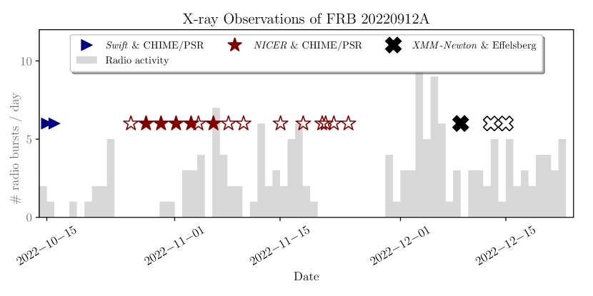
Figure 1: Timeline of X-ray observations compared with the number of bursts detected by CHIME/FRB per few-minute daily source transit (gray histogram, not corrected for exposure). The observations are summarized in more detail in Section 2. The blue triangles and red stars represent Swift  and NICER  observations, respectively, for which CHIME/Pulsar provided simultaneous radio coverage. The black crosses denote our XMM-Newton  observations with contemporaneous Effelsberg  radio coverage. Filled markers denote observations with radio bursts detected during a GTI during an X-ray observation. These X-ray data were obtained during periods of high radio activity from the source.

3 Analysis

3.1 Persistent X-ray Emission

We detect no persistent source consistent with FRB 20220912A’s position (Hewitt et al., 2024) in the XMM-Newton EPIC data (within a 90% containment region, which is 680 pixels or 35 arcseconds). In order to determine the significance of a collection of X-ray photons or lack thereof, we use the methodology presented by Kraft et al. (1991), who derived a Bayesian expression for confidence intervals in error analysis for photon counting experiments with low numbers of counts. This formalism is often chosen by X-ray astronomers because of its straightforward application to circumstances with non-zero expected background counts. We make use of the Python implementation in the pwkit library (Williams et al., 2017) in order to compute these statistics. We estimate a 99.7% credible interval (chosen as it produces physically relevant constraints while still being conservative, 99.7% is $\sim 3\sigma$ Gaussian equivalent) on the 0.5–10.0 keV source count rate from the EPIC pn of between 0 and $5\times 10^{-4}$ counts per second for the $\sim$ 44 ks GTIs within our observations of the source. This 99.7% credible interval upper limit count rate assumes an average background rate of $3\times 10^{-3}$ counts per second, which was estimated from the same observations in a spatial region away from FRB 20220912A and without any obvious X-ray sources. Hence we infer a 99.7% credible interval upper limit on unabsorbed flux of ${8.8}\times 10^{-15}$ ergs cm^-2 s^-1 in the 0.5–10 keV range, assuming isotropic emission with ${\Gamma=2}$ power-law spectrum, absorbed by a $N_{H}=10^{22}$ cm^-2 neutral hydrogen column. Using the luminosity distance of 362.4 Mpc, this corresponds to a 0.5–10.0 keV isotropic-equivalent luminosity of ${L_{X}<1.4\times 10^{41}}$ ergs s^-1. The correct $N_{H}$ to assume is not obvious. X-rays could be significantly absorbed by intervening material along the line-of-sight of our source. From our own Galaxy, HI4PI Collaboration et al. (2016) estimate a neutral hydrogen column of $1.42\times 10^{21}$ cm^-2 along the line of sight of FRB 20220912A. This can be an estimate of the minimal possible total $N_{H}$ along the line of sight of the source. Following the argument in Scholz et al. (2020), the low extragalactic DM of 94.3 or 97.3 pc cm^-3 (using the free electron models in NE2001, YWM16 respectively, Cordes & Lazio 2002; Yao et al. 2017) suggests there are not orders of magnitude more ionized plasma along the line of sight than what is contributed by our Galaxy. He et al. (2013) predict  $(3\pm 1)\times 10^{21}$ cm^-2 from this extragalactic DM, after accounting for the uncertainty in the relationship and the differing extragalactic DM predictions. To be conservative, we assume an $N_{H}$ of $10^{22}$ cm^-2 throughout. Of course, this makes the assumption that the ratio of atomic metals to free electrons is similar to that found in the MW interstellar medium along the entire line of sight. This may not be the case local to the FRB source if, for example, the source was located in a decades-old supernova remnant (Metzger et al., 2017). If there was extreme X-ray absorption local to the source, one could expect a $N_{H}$ value as high as $10^{24}$ cm^-2 (Scholz et al., 2017), although such a scenario has been disfavoured for at least some FRB sources, given their detection at low ($\sim 300$ MHz) frequencies (Chawla et al., 2022; Scholz et al., 2020). FRB 20220912A has been detected at frequencies as low as 111 MHz, so the same argument can be applied to this source (Fedorova et al., 2023). The impact of an extreme X-ray absorption on resultant X-ray limits is explored more in Scholz et al. (2017, 2020), and from their calculations, we can assume in this scenario our limits would be about an order of magnitude less constraining.

Swift-XRT also did not detect significant persistent source within the 90% containment region of FRB 20220912A  (a circle with a 20 pixel or 47 arcsecond radius), which places an upper bound of the 99.7% credible interval on absorbed source flux between 0.2 and 10.0 keV of $8.5\times 10^{-14}$ erg cm^-2 s^-1. Again, this assumes an average background rate, here $1\times 10^{-3}$ counts per second, which we estimate from a spatial region away from FRB 20220912A without any obvious X-ray sources in it. We report this less constraining value along with the deep limit from XMM-Newton EPIC as the Swift-XRT limit was obtained much closer to the source’s initial activation, and hence could still be constraining for decaying emission models.

We do not estimate the NICER persistent upper limit as we detected another faint source with Swift-XRT (0.2–10.0 keV X-ray flux $\sim 6\times 10^{-14}$ erg cm^-2 s^-1 using the On-Demand XRT products webtool from Evans et al. 2009) within the FoV of the NICER observations (albiet off-axis) and NICER  is non-imaging. The faint source is not consistent with FRB 20220912A  as it is outside of Swift-XRTs 90% PSF containment region around FRB 20220912A.

We searched a two degree radius around FRB 20220912A  for any gamma-ray source in the Fermi-LAT 14-Year Point Source Catalog (4FGL-DR4; Ballet et al., 2023; Abdollahi et al., 2022); but there are no known cataloged gamma-ray sources within this sky region.

3.2 Prompt X-ray Emission at the Times of Radio Bursts

XMM-Newton

We detected one radio burst during our XMM-Newton observations. The burst occurred during a time of high X-ray background, presumably from soft proton flares. We place a 99.7% credible region upper limit of 5.8 counts given the absence of photons detected by EPIC-pn (using Kraft et al. 1991), or $<{1.5\times 10^{-10}}$ erg cm^-2 on 0.5–10.0 keV unabsorbed X-ray fluence at the time of the radio burst (having corrected for the DM delay). The background rate for each of the short duration/burst upper limits is estimated by averaging the light curve over the 200s surrounding the radio burst ToA, with a buffer equal to the assumed duration of the X-ray burst. For XMM-Newton and Swift, we average over the light curve of the 90% spatial containment region of FRB 20220912A, whereas for NICER, which is non-imaging, we average over the light curve of the entire field. The upper limit value also assumes a 100 ms X-ray burst duration, photo-electrically absorbed by a moderate neutral hydrogen column in that direction (${N_{H}=10^{22}}$ cm^-2), assuming a 10 keV blackbody spectrum. A timescale of 100 ms was chosen as it is comparable to the duration of the X-ray counterpart to the SGR 1935+2154 April 2020 FRB-like radio burst (Mereghetti et al., 2020). There are no photons within $\pm$ 820 ms of the burst (after correcting for the dispersive delay), hence a similar limit can be placed for bursts of durations up to 820 ms.

NICER

We detected 26 radio bursts with CHIME/Pulsar while NICER  was simultaneously observing the source. Of these bursts, and considering the trials factor of 26, the smallest individual 99.7% credible region upper limit constrains a prompt 0.5–10.0 keV X-ray burst fluence to 9.0 counts, or $<{4.0}\times 10^{-10}$ erg cm^-2 assuming the same burst properties as for XMM-Newton  above. The depth of the limit, for a fixed telescope and source distance, is predominantly based on the average background rate at the time the limit is placed. In placing the best limit, we are essentially selecting for the lowest background, and hence we must incorporate a trials factor to reflect the increased probability of observing a low background count rate realization compared to the true background count rate among many trials. The limit reported above is corrected for 26 trials via the Dunn–Šidák correction(Šidák, 1967), a simple method to control for the family-wise error rate in multiple hypothesis testing which is conservative for tests that are positively dependent. The Dunn–Šidák correction widens the confidence intervals for a given significance threshold ($\alpha\in[0,1]$) to $100\dot{(}1-\alpha)^{1/m}$ where $m\in\mathbb{N}$ is the number of hypotheses/trials being tested.

Swift

We detected three radio bursts with CHIME/Pulsar while Swift  was simultaneously observing the source. Of these bursts, and considering the trials factor here of three, the smallest individual 99.7% credible region upper limit constrains a prompt 0.5–10.0 keV X-ray burst fluence to 6.9 counts, or $<{1.4}\times 10^{-9}$ erg cm^-2 assuming the same burst properties as for XMM-Newton  and NICER  above.

3.3 Bursts/Flares of Varying Durations at Other Times During the Observations

We carried out an untargeted search for bursts of varying durations at times other than at the time of radio bursts during the observations. We searched for significant signals above background from X-ray photons coming from the location of FRB 20220912A  (i.e., within the 90% PSF-containment regions of Swift-XRT and XMM-Newton  or any NICER photons, as it is non-imaging). The search was performed by binning the data according to burst width and then checking if the number of photons in a given bin was statistically significant at the 99.7% level according to the statistics presented by Kraft et al. (1991). We used an estimate of the background by averaging the count rate nearby in time to the bin of interest (with a few-bin padding on either side in case a hypothetical burst arrived between two neighboring time bins). We then correct for the problem of multiple hypotheses (or the look-elsewhere effect) with the Dunn–Šidák correction (Šidák, 1967). The assumed trials factor is equal to the sum of the number of bins checked for significant signal over all tested bin widths. We searched for bursts with durations of 1 ms, 10 ms, 100 ms, 1 s and 10 s. We find no significant bursts across all X-ray instruments and observations (99.7% credible region), and we would have been sensitive to bursts at these timescales with $0.5-10.0$ keV fluences $\sim 10^{-9}$ erg cm^-2.

3.4 Stacked Prompt Search

Previous methodologies

While the existing formalism of Kraft et al. (1991) allows us to place limits on X-ray emission at the time of each radio burst, the authors do not provide a formalism for the case where multiple independent measurements are taken of a given source. Scholz et al. (2017) and Piro et al. (2021) combine the information from multiple independent trials, that is, multiple non-detections of X-ray emission at the time of radio bursts, by assuming that an X-ray burst of the same energy is emitted at the time of each detected radio burst. We derive the Bayesian expression for this calculation in Appendix A. This model assumes that the independent observations of $N_{i}$ X-ray counts at the time of a radio burst is described by a Poisson model with rate parameter $\lambda_{i}=S+B_{i}$. For $n$ total X-ray observations, $i\in 1,\ldots n$ is an index describing the $i^{\text{th}}$ X-ray observation. $B_{i}$ are the average background rates in each observation and $S$ is the average source count rate during the bursts. The $B_{i}$ are treated as known and constant. That is,

$$N_{i}\sim\text{Poisson}(\lambda_{i}=S+B_{i}).$$

New methodology

All bursts having the same luminosity is a strong assumption, however, given that most astrophysical transient phenomena that we see can be characterized by some luminosity distribution.

A more conservative assumption is that an X-ray burst of the same relative X-ray-to-radio fluence is emitted at the time of each radio burst. That is, we ask the question: if one expects to see an X-ray burst whose luminosity scales proportionally to that of a simultaneous radio burst, what is the limit that can be placed? We derive a hierarchical Bayesian expression for the X-ray-to-radio fluence ratio $\eta_{\text{\,x/r}}=F_{\text{X-ray}}/F_{\text{radio}}$ in Appendix B. $F_{\text{X-ray}}$ is the X-ray fluence (in erg cm^-2), $F_{\text{radio}}$ is the radio fluence (converted from Jy ms to erg cm^-2 Hz^-1 and then multiplied by the emitting bandwidth of the bursts, which can be a conservative underestimate due to our finite observing band). This hierarchical model assumes the following distributions

Step I $$N_{i} \sim\text{Poisson}(\lambda_{i}=S_{i}+B_{i})$$

Step II $$S_{i} \sim\mathcal{N}_{0}^{\infty}\left(\frac{\eta_{\text{\,x/r}}F_{\text{radio},i}}{(\text{Flux/S})},\frac{\eta_{\text{\,x/r}}\sigma_{F_{\text{radio},i}}}{(\text{Flux/S})}\right)$$

where $F_{\text{radio, }i},\sigma_{F_{\text{radio, }i}}$ are the radio fluences of the detected simultaneous bursts and their associated uncertainties, respectively. (Flux/S)$\in\mathbb{R}^{+}$ is a conversion parameter to turn the X-ray count rates into fluences. This value depends on the underlying spectral model assumed and the effective area of the X-ray telescope, but can be computed using standard X-ray tools. $\mathcal{N}_{0}^{\infty}(\mu,\sigma)$ denotes a normal distribution truncated on the left at $0$ with mean $\mu\in\mathbb{R}^{+}$ and standard deviation $\sigma\in\mathbb{R}^{+}$. Poisson$(\lambda)$ denotes the Poisson distribution with rate parameter $\lambda\in\mathbb{R}^{+}$. With CHIME/Pulsar alone, we have only a lower limit on burst fluence, but co-detections between CHIME/Pulsar and other telescopes suggest a factor of 2–3 underestimate. Hence, for these bursts, we instead model the flux distribution in Step II as $\mathcal{N}_{S_{\text{radio, }i}}^{\infty}(2S_{\text{radio, }i},S_{\text{radio, }i})$ where $S_{\text{radio, }i}=\eta_{\text{\,x/r}}F_{\text{radio, }i}/(\text{Flux/S})$. This enforces that our reported fluence limits are strict lower limits, and conservatively accounts for the underestimate factor of 2–3. The resulting limits are conservative because they, on average, underestimate the fluence of the CHIME/Pulsar radio bursts, and hence inflate the upper limit we place on $\eta_{\text{\,x/r}}$. A numerical implementation of these models in python and a minimal working example is available on Zenodo at https://doi.org/10.5281/zenodo.12785591 (Cook et al., 2024).

For all 30 radio bursts from FRB 20220912A  that were detected during our X-ray observations, we compute this stacked upper limit of $2\times 10^{6}$ on $\eta_{\text{\,x/r}}$ at the 99.7% credible level, assuming our conservative 10 keV blackbody burst spectrum. The posterior distribution of this model is derived in full in Appendix B. The observed SGR 1935-2154 X-ray burst associated with FRB-like emission was modelled with a cutoff powerlaw at $E_{\text{cut}}=83.89$ keV, photon index $\Gamma=1.56$ (Li et al., 2021). If we instead assume this spectrum for our burst model, and after having corrected for absorption, we derive an upper limit on $\eta_{\text{\,x/r}}$ of ${8\times 10^{5}}$ at the 99.7% credible level. We show the posterior distributions on $\eta_{\text{\,x/r}}$ using this method in the top right panel of Figure 2 and compare with previous ‘bona fide’ counterpart limits in Figure 3. For the 2004 December 27 magnetar giant flare of SGR 1806-20, Tendulkar et al. (2016) placed upper limits on the possible radio fluence at the time of the 1.4 erg cm^-2 X-ray flare given the non-detection with the Parkes radio telescope, which was observing a location 35.6 degrees away from the source at the time (Hurley et al., 2005; Palmer et al., 2005; Terasawa et al., 2005). This corresponds to a lower-limit on X-ray-to-radio fluence ratio, given it is an upper limit on the radio fluence which is the denominator, of $4\times 10^{10}$ for X-ray counterparts of FRBs if they can be attributed to magnetar giant flares like that observed for SGR 1806-20. However, the majority of upper limits placed in that paper are incompatible with our limits and all published limits on $\eta_{\text{\,x/r}}$ to date.

Using the formalism derived in Appendix B, we revisit the limits placed by Scholz et al. (2017); Pilia et al. (2020); Scholz et al. (2020), and Yan et al. (2024). This allows a more direct comparison between the limits, compiles all the data in one place, and decreases the upper limit placed on $\eta_{\text{\,x/r}}$ for each work. For the aforementioned papers, Table 4 summarizes the data that are required to calculate our stacked $\eta_{\text{\,x/r}}$ constraint (Equation B9). The full posterior distributions from the retreatment of these soft-X-ray data are shown in Figure 2. The corresponding 99.7% credible intervals on $\eta_{\text{\,x/r}}$ from these data, using our method, are also placed in the broader context of observing frequency-$\eta_{\text{\,x/r}}$ phase space in Figure 3.

The stacked $\eta_{\text{\,x/r}}$ limit placed on FRB 20180916B  plotted in Figure 3 uses the observations of Scholz et al. (2017) and Pilia et al. (2020). The limit could be improved by the inclusion of limits placed by Trudu et al. (2023), but the required data are not currently public.

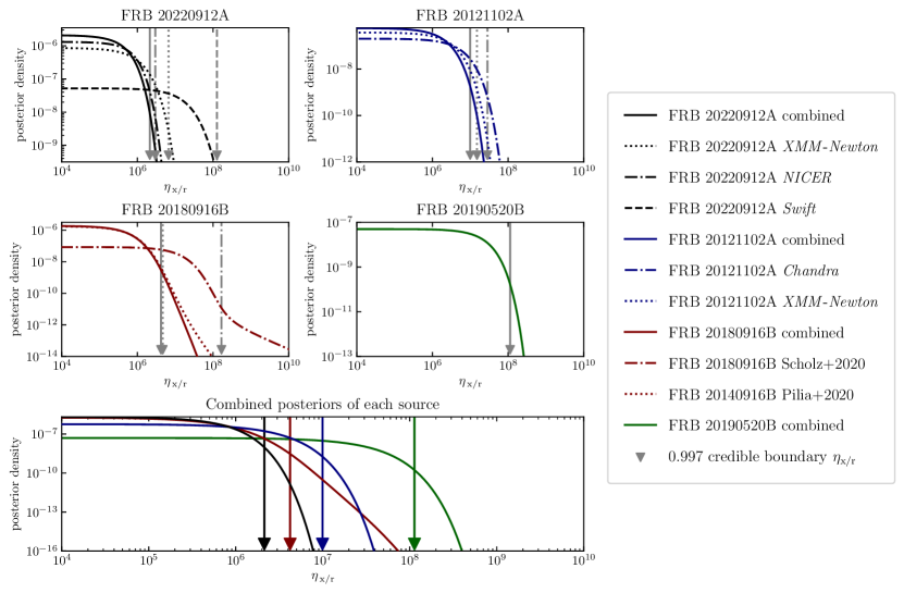
Figure 2: Posterior distributions of $\eta_{\text{\,x/r}}$ (band-integrated X-ray-to-radio fluence ratios) from a selection of soft X-ray observations of FRBs. In the top four panels, the value of $\eta_{\text{\,x/r}}$ corresponding to the upper boundary on the 0.997 credible interval is shown with a gray arrow using the same linestyle. The posterior distributions approach a constant value from the lower $\eta_{\text{\,x/r}}$ bound of the plot to $\eta_{\text{\,x/r}}=0$ and approach zero density as $\eta_{\text{\,x/r}}$ approaches infinity. Top-left panel: Posterior distributions on $\eta_{\text{\,x/r}}$ using the Bayesian stacking method described in Section 3.4 and Appendix B, based on all observations reported in this paper (solid black line). The posterior distribution of $\eta_{\text{\,x/r}}$, computed from simultaneous XMM-Newton and Effelsberg data at the time of B30, is shown as a black dotted line. The dot-dashed line shows the posterior distribution of $\eta_{\text{\,x/r}}$, computed from simultaneous NICER and CHIME/Pulsar bursts (B4–B29). The dashed line shows the posterior distribution of $\eta_{\text{\,x/r}}$, computed from the simultaneous Swift and CHIME/Pulsar bursts (B1–B3). Top-right panel: Posterior distributions of four radio bursts from FRB 20121102A simultaneously observed with Chandra, reported by Scholz et al. (2017), and combined using our method (solid blue line). Middle-left panel: Same as in the top panels, but instead using the observations reported by Scholz et al. (2020) (dotted maroon line) and Pilia et al. (2020) (dot-dashed maroon line), along with our combined Bayesian stacking measurement (solid maroon line). Middle-right panel: Same as in the top panels, but instead based on the observations of FRB 20190520B by Yan et al. (2024) and combined using our Bayesian stacking method (solid green line). Bottom panel: Cumulative posterior distributions of $\eta_{\text{\,x/r}}$, combined using our Bayesian stacking method and plotted source-by-source, for comparison. Arrows, colored by source, denote upper limits corresponding to 0.997 $\eta_{\text{\,x/r}}$ credible regions.

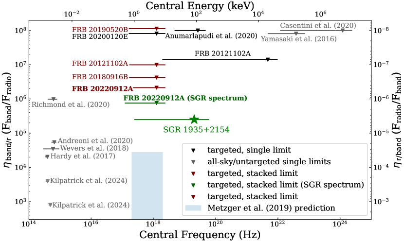
Figure 3: Upper limits placed on the band-integrated HE-to-radio fluence $(F)$ ratio ($\eta_{\text{band/r}}=F_{\text{band}}/F_{\text{Radio}}$, since we also consider measurements outside of the X-ray band) for optical, UV, X-ray and gamma-ray observations during simultaneous radio observations of FRBs, adapted from Chen et al. (2020). For FRB 20220912A , the limit presented is calculated using the Bayesian method described in Appendix B, considering all 30 upper limits at the time of radio bursts and assuming a 10 keV blackbody burst spectrum. For consistency, we present upper limits from previously reported non-detections combined using the Bayesian stacking method presented in this paper (maroon lines, bold text to indicate the values derived from our observations). Other relevant X-ray and gamma-ray limits, based on targeted observations, are shown as black lines (Scholz et al., 2017; Anumarlapudi et al., 2020; Pearlman et al., 2023). Previous constraints from untargeted observations are labeled by publication in gray (Andreoni et al., 2020; Casentini et al., 2020; Hardy et al., 2017; Richmond et al., 2020; Scholz et al., 2017, 2020; Wevers et al., 2018; Yamasaki et al., 2016). We show the measured $\eta_{\text{\,x/r}}$ of the X-ray burst observed contemporaneously with FRB-like emission from Galactic magnetar SGR 1935+2154 detected on 2020 April 28 (green star; Li et al. 2021) and the forest green line shows our stacked $\eta_{\text{\,x/r}}$ limit assuming the observed burst spectrum of this SGR 1935+2154 X-ray burst (Li et al., 2021). The predicted parameter space of $\eta_{\text{\,x/r}}$ for a $\sim$keV-energy young magnetar burst (Metzger et al., 2019), assuming a luminosity distance of 362.4 Mpc for FRB 20220912A  and the observed radio fluence of radio burst B30, is shown in blue.

4 Discussion

We now discuss each of the limits derived from our observations in the context of known transient populations and predictions from FRB models. Metzger et al. (2019) predict an 1–10 keV X-ray counterpart with luminosity $10^{42}$–$10^{43}$ erg s^-1 for their model of FRBs as synchrotron maser emission from decelerating relativistic blast waves. When one places this emission, predicted to last 0.1–1 seconds, at the distance of FRB 20220912A , it corresponds to fluences in the range $(6-600)\times 10^{-15}$ erg cm^-2.

Our most constraining 99.7% credible region upper limit on X-ray emission at the time of a radio burst from FRB 20220912A, $1.5\times 10^{-10}$ erg cm^-2, does not yet probe this region. However, our simultaneous X-ray and radio measurements of the hyperactive, bright FRB 20220912A allow us to place the best $\eta_{\text{\,x/r}}$ constraints in the X-ray band to date. Our lowest 99.7% $\eta_{\text{\,x/r}}$ upper limit is ${7\times 10^{6}}$, and when stacking data from the time of each of our radio bursts, is $2\times 10^{6}$. While the limits in this paper are not the most constraining in X-ray burst luminosity placed for an FRB to date, owing to the larger distance of FRB 20220912A  compared to FRB 20200120E (Pearlman et al., 2023), our limits remain highly relevant because the hyperactivity and brightness of the source allow us to place deeper limits on $\eta_{\text{\,x/r}}$.

Our observations cannot rule out magnetospheric models, which, if they predict an X-ray counterpart, cite expected $\eta_{\text{\,x/r}}$ from $\sim$ 1 (comparable energy to that of the radio burst, e.g., Margalit et al. 2020) to $\eta_{\text{\,x/r}}\sim 10^{4}$ (Lu et al., 2020). Drawing on analogies with solar flares, Lyutikov (2002) hypothesized that bursts from magnetars could produce an X-ray-to-radio fluence ratio of $\sim 10^{4}$ (this model was later employed as an explanation of FRBs by Popov & Postnov 2010). This analogy was recently further contextualized for the microshots emitted by this source, FRB 20220912A, by Hewitt et al. (2023). Our best $\eta_{\text{\,x/r}}$ limit is the closest yet to the $\eta_{\text{\,x/r}}=2.5\times 10^{5}$ observed for the FRB-like burst on 2020 April 28 from SGR 1935+2154 and accompanying X-ray burst (CHIME/FRB Collaboration, 2020; Bochenek et al., 2020; Mereghetti et al., 2020; Li et al., 2021). Indeed, for a similar X-ray burst spectrum (a cutoff powerlaw at $E_{\text{cut}}=83.89$ keV, photon index $\Gamma=1.56$, and after having corrected for galactic absorption; Li et al. 2021), instead of our conservative 10 keV blackbody burst spectrum, the stacked $\eta_{\text{\,x/r}}$ limit is $\mathbf{8}\times 10^{5}$, only a factor of 3 from the observed $\eta_{\text{\,x/r}}$ of the FRB-like burst from SGR 1935+2154. This motivates the continued search for X-ray counterparts for FRB sources. After a statistically significant number of bright radio bursts like those detected from FRB 20220912A, one could disfavor the mechanism producing the SGR 1935+2154 simultaneous X-ray and radio burst for a given repeater source if no X-ray emission was seen, under the assumption that an X-ray burst with equal $\eta_{\text{\,x/r}}$ is emitted with each radio burst. Considering simultaneous XMM-Newton  and Effelsberg  observations like the campaign in this paper, $\eta_{\text{\,x/r}}\sim 10^{4}$ could be measured with our Bayesian method at the 99.7% level given an X-ray non-detection of two kJy ms radio bursts, ten 500 Jy ms radio bursts, or fifty 50 Jy ms radio bursts. Highly energetic bursts from repeaters are detected more rarely, but they have been observed before (Kirsten et al., 2024).Hewitt et al. (2023) and Ould-Boukattine et al. (2022) report a handful of bursts from FRB 20220912A  with radio fluences $>400$ Jy ms and as high as 972 Jy ms. Ikebe et al. (2023) report a burst from FRB 20201124A with fluence $>189$ Jy ms.

In 2020 October, SGR 1935+2154 was observed to emit regular pulsed radio emission, with radio bursts detected with luminosities comparable to typical rotating radio transients or radio pulsars, depending on which distance was assumed (Zhu et al., 2023). This pulsed radio emission was anti-aligned with the X-ray pulsed emission at the time (Younes et al., 2023). We computed the fraction of X-ray-to-radio energy released during an average single-pulse, and find this $\eta_{\text{\,x/r}}$ of $\sim(7-12)\times 10^{6}$, which can be ruled out for FRB 20220912A  by our observations (Zhu et al., 2023; Younes et al., 2023).

Given that FRB 20220912A  and FRB 20180916B  have source distances of the same order of magnitude, and were observed with the same telescopes at the times of radio bursts, the upper limit we derive on persistent X-ray emission at the location of FRB 20220912A  is similar in magnitude to that derived for FRB 20180916B  (Scholz et al., 2020). Thus we can derive similar conclusions about the nature of the source. A Crab-like nebula, which has persistent X-ray luminosity $\sim 10^{37}$ erg s^-1, cannot be ruled out for the source. Our limit is lower than the luminosities of most ULXs, but we cannot rule out luminosities in the range of Galactic HMXBs and LMXBs (Terashima & Wilson, 2003; Sazonov & Khabibullin, 2018; Earnshaw et al., 2019; Pearlman et al., 2023).

5 Conclusions

High energy studies of FRB counterparts are crucial to derive a full picture of the spectral properties of FRBs, and hence not only to disentangling the sources of FRBs but also as a probe of one the most extreme radio transients in the Universe. CHIME/FRB is a unique monitor of stochastic repeater activity, which is often clustered in time (e.g., Collaboration, 2020; Lanman et al., 2022; Shin & CHIME/FRB Collaboration, 2024). Such a monitor allows coordination of HE observations with the maximum probability of detecting contemporaneous radio bursts— this, along with the Bayesian stacking methodology presented in this paper enables searches in new areas of counterpart relative-fluence ($\eta_{\text{\,x/r}}$) phase space.

The recently hyper-activated FRB 20220912A  is an example that shows the power of these types of observations. Based on an extensive, contemporaneous radio and X-ray campaign, we report our lowest single 99.7% credible upper limit on $\eta_{\text{\,x/r}}$ of ${7\times 10^{6}}$, which is the lowest constraint yet. Using a hierarchical extension to the standard Bayesian treatment of low-count, background contaminated data, we combined information from X-ray non-detections at the times of 30 of radio bursts from FRB 20220912A. This allowed us to constrain $\eta_{\text{\,x/r}}<2\times 10^{6}$ at the 99.7% level, assuming all bursts are associated with X-ray bursts with the same fluence ratio. Our brightest radio burst observed simultaneously with an X-ray telescope produces a 99.7% credible region 0.5–10.0 keV fluence limit of ${1.5\times 10^{-10}}$ erg cm^-2 assuming a 100ms-burst with a 10 keV blackbody spectrum, corrected for absorption by a ${10^{22}}$ cm^-2 neutral hydrogen column. Our XMM-Newton  observations constrain, at the 99.7% level, persistent flux from FRB 20220912A  to less than ${8.8\times 10^{-15}}$ ergs cm^-2 s^-1 in the 0.5–10-keV range assuming a powerlaw spectrum with $\Gamma=2$ after correcting for absorption by a ${10^{22}}$ cm^-2 neutral hydrogen column. At the luminosity distance of 362.4 Mpc, this corresponds to a 0.5–10.0 keV luminosity of $L_{X}<{1.4\times 10^{41}}$ ergs s^-1.

Continued arcsecond localizations from projects like the Deep Synoptic Array-110 (DSA-110) and the upcoming CHIME/FRB Outriggers will allow us to target the most active, nearby, and energetic of FRB sources for HE follow-up campaigns like the one detailed in this paper (Bhardwaj et al. 2023; Law et al. 2024; Lanman et al. 2024). This will allow the ongoing pursuit of source-discriminating HE emission closer to the luminosities predicted by many models and observed transient behavior from magnetars in our own Galaxy (e.g., see Pearlman et al. 2023).

Appendix A Bayesian formalism for source rate constraints from multiple observations

We seek to combine information from $n$ X-ray observations at the time of radio bursts, which can be treated as independent trials if sufficiently separated in time (i.e., the time between the FRBs is long compared to the durations tested). We follow the Kraft et al. (1991) Bayesian formalism, but construct the posterior distribution probability using Bayes rule assuming $n$ observations of $N_{i}$ X-ray photons for $(i\in 1,\ldots n)$, and (known) average background rates of $B_{i}$ for $(i\in 1,\ldots,n)$, to estimate a rate $S$ for X-ray emission at the time of radio bursts. This method assumes that $S$ is constant for all radio bursts, during the radio bursts themselves. From Bayes rule, we can derive the posterior distribution $f$ on the rate $S$:

$$p(S) \propto 1$$ (A1)

$$N_{i} \sim\text{Poisson}(\lambda_{i}=B_{i}+S)$$ (A2)

$$f(S|N_{1},\ldots,N_{n}) =\frac{P(N_{1},\ldots,N_{n}|S)p(S)}{P(N_{1}\ldots,N_{n})}$$ (A3)

$$\propto\prod_{i=1}^{n}\text{Poisson}(N_{i}|\lambda_{i}=B_{i}+S),$$ (A4)

where $\text{Poisson}(k|\lambda)$ is the Poisson probability mass function of $k\in\mathbb{N}$ observed counts given Poisson rate $\lambda\in\mathbb{R}^{+}$ and $B_{i}$ is assumed constant and known for each observation $n$. Kraft et al. (1991) assume an improper uniform prior distribution p(S) = c for all positive values. In order to construct a proper (finite) uniform prior distribution, one should instead assume $p(S)=c\ \forall S\in[0,x]$ for some appropriately large value $x\in\mathbb{R}^{+}$ of X-ray rate, and practically, this will be enforced by any analytic implementation which computes this posterior distribution. Previous limits placed on the X-ray emission at the time of FRBs can instead be used to set a conservative but still informative prior distribution. In order to construct the 99.7% credible interval from this equation, again following Kraft et al. (1991), we enforce that the difference in the flux bounds of the credible interval ($S_{\text{max}}-S_{\text{min}}$) is minimized and the peak value of the posterior density distribution is included. This is known as the highest posterior density interval (see, e.g., chapter one of Stenning & van Dyk, 2018, for applications in astronomy).

Appendix B Bayesian formalism for $\eta_{\text{\,x/r}}$ constraints from multiple observations

In Appendix A, we assume a single source rate, $S$, and calculate the posterior distribution on that source rate by combining information from multiple observations. If one expects that the X-ray fluence from the source should be proportional to the radio fluence, it is desirable to estimate the posterior distribution on the relative X-ray to radio source fluence, $\eta_{\text{\,x/r}}$. We thus assume here that $\eta_{\text{\,x/r}}$ is constant for all bursts, and that $S_{i}$ can vary. Again, we define $N_{i}$ as the number of X-ray photons at the time of each radio burst, $B_{i}$ is the average background rate of X-ray photons at the time of each radio burst and $F_{\text{radio, }i}$ is the calculated radio fluence, with associated error $\sigma_{F_{\text{radio, }i}}$. What is the credible interval on $\eta_{\text{\,x/r}}$ for these multiple observations? In the following derivation, we use $N_{i},B_{i},F_{i}$ as shorthand for the more conventional general list $N_{0},B_{0},F_{0},\ldots,N_{n},B_{n},F_{n}$ where $n$ is the total number of detected bursts. We will compute the posterior distribution of the observations given following model, introduced in Section 3.4:

Level I $$N_{i} \sim\text{Poisson}(\lambda_{i}=S_{i}+B_{i})$$ (B1)

Level II $$S_{i} \sim\mathcal{N}^{\infty}_{0}\left(\frac{\eta_{\text{\,x/r}}F_{\text{radio},i}}{(\text{Flux/S})},\frac{\eta_{\text{\,x/r}}\sigma_{F_{\text{radio},i}}}{(\text{Flux/S})}\right),$$ (B2)

where (Flux/S)$\in\mathbb{R}^{+}$ is a conversion parameter to turn the X-ray count rates into fluxes. This value depends on the underlying spectral model assumed and the effective area of the X-ray telescope, but can be computed using standard X-ray tools. We assume a blackbody spectral model with $kT=10$ keV for the bursts and present the corresponding (Flux/S) parameter for each observation in Table 4. $\mathcal{N}_{0}^{\infty}(\mu,\sigma)$ denotes a normal distribution truncated on the left at $0$ with mean $\mu\in\mathbb{R}$ and standard deviation $\sigma\in\mathbb{R}^{+}$. The truncation is introduced because negative source counts are not physical. Poisson$(\lambda)$ denotes the Poisson distribution with rate parameter $\lambda\in\mathbb{R}^{+}$. The $B_{i}$ are treated as known and fixed, but an additional model for the error can be added in Level II if there are significant uncertainties in this estimation or the background rate is variable. Starting again from Bayes rule, we can write the posterior distribution distribution $f(\eta_{\text{\,x/r}})$

$$f(\eta_{\text{\,x/r}}) =\frac{p(N_{i}|\eta_{\text{\,x/r}})p(\eta_{\text{\,x/r}})}{C},$$ (B3)

where $C\in\mathbb{R}$ is some normalization constant. To compute the probability density of the observed counts, we must invoke an X-ray rate parameter for each observation, $S_{i}$, however this value is not known. Instead, we assume a hierarchical Bayesian model, introducing $S_{i}$ as a random variable in the following equation using the chain rule of probability through the identity $p(A|B)=\int_{C}p(A,C|B)\differential C=\int_{C}p(C|B)p(A|B,C)\differential C$ for random variables $A,B,C$:

$$f(\eta_{\text{\,x/r}}) =\frac{1}{C}p(\eta_{\text{\,x/r}})\int_{S_{1}}\int_{S_{2}}\ldots\int_{S_{n}}p(N_{i}|S_{i},\eta_{\text{\,x/r}})p(S_{i}|\eta_{\text{\,x/r}})\differential S_{1}\differential S_{2}\ldots\differential S_{n}$$ (B4)

$$\propto p(\eta_{\text{\,x/r}})\int_{S_{1}}\int_{S_{2}}\ldots\int_{S_{n}}p(N_{i}|S_{i},\eta_{\text{\,x/r}})p(S_{i}|\eta_{\text{\,x/r}})\differential S_{1}\differential S_{2}\ldots\differential S_{n}$$ (B5)

$$\propto p(\eta_{\text{\,x/r}})\int_{S_{1}}\int_{S_{2}}\ldots\int_{S_{n}}\prod_{i}\text{Pois}(N_{i}|\lambda_{i}=S_{i}+B_{i})\hskip 4.2679pt\mathcal{N}^{\infty}_{0}\left(\frac{\eta_{\text{\,x/r}}F_{\text{radio},i}}{(\text{Flux/S})},\frac{\eta_{\text{\,x/r}}\sigma_{F_{\text{radio},i}}}{(\text{Flux/S})}\right)\differential S_{1}\differential S_{2}\ldots\differential S_{n}$$ (B6)

$$\propto p(\eta_{\text{\,x/r}})\prod_{i}\int^{\infty}_{0}\hskip 4.2679pt\frac{(\text{Flux/S})(B_{i}+S_{i})^{N_{i}}}{\sqrt{2\pi}\eta_{\text{\,x/r}}\sigma_{F_{\text{radio},i}}(N_{i}!)}\exp[-\left(B_{i}+S_{i}+\frac{(\text{Flux/S})^{2}\left(S_{i}-\frac{\eta_{\text{\,x/r}}F_{\text{radio},i}}{(\text{Flux/S})}\right)^{2}}{2\eta_{\text{\,x/r}}^{2}\sigma^{2}_{F_{\text{radio},i}}}\right)]\differential S_{i}$$ (B7)

$$\propto p(\eta_{\text{\,x/r}})\exp(-\sum_{i=1}^{n}B_{i})\prod_{i=1}^{n}\int^{\infty}_{0}\hskip 4.2679pt\frac{(\text{Flux/S})(B_{i}+S_{i})^{N_{i}}}{\sqrt{2\pi}\eta_{\text{\,x/r}}\sigma_{F_{\text{radio},i}}(N_{i}!)}\exp[-\left(S_{i}+\frac{(\text{Flux/S})^{2}\left(S_{i}-\frac{\eta_{\text{\,x/r}}F_{\text{radio},i}}{(\text{Flux/S})}\right)^{2}}{2\eta_{\text{\,x/r}}^{2}\sigma^{2}_{F_{\text{radio},i}}}\right)]\differential S_{i}$$ (B8)

$$\propto p(\eta_{\text{\,x/r}})\prod_{i=1}^{n}\int^{\infty}_{0}\hskip 4.2679pt\frac{(B_{i}+S_{i})^{N_{i}}}{\eta_{\text{\,x/r}}}\exp[-\left(S_{i}+\frac{(\text{Flux/S})^{2}\left(S_{i}-\frac{\eta_{\text{\,x/r}}F_{\text{radio},i}}{(\text{Flux/S})}\right)^{2}}{2\eta_{\text{\,x/r}}^{2}\sigma^{2}_{F_{\text{radio},i}}}\right)]\differential S_{i}.$$ (B9)

This expression can be numerically integrated directly and normalized, or estimated with MCMC methods. We use the posterior distribution from a previous independent trial as our prior distribution when stacking.

The reported credible regions correspond to the highest posterior density interval. A numerical implementation of this integral in python and a minimal working example is available on Zenodo at https://doi.org/10.5281/zenodo.12785591, (Cook et al., 2024)

Table 4: Summary of observations from previous X-ray counterpart searches of FRBs. All values are reported for an X-ray observing band $0.5-10.0$keV. In all studies, there are no X-ray photons detected coincident with the source position within 100 ms of each burst. The corresponding stacked $\eta_{\text{\,x/r}}$ credible interval upper limits can be found in Figure 3. All arrival times are barycentric and corrected to infinite frequency. We assume an error of 10% on the fluences of Scholz et al. (2017). Yan et al. (2024) report only the radio burst energy, and hence we estimate the radio burst fluence assuming the full bandwidth of FAST, 400 MHz. The multiwavelength campaigns of Piro et al. (2021) and Trudu et al. (2023) are also appropriate for direct comparison here, however the summary statistics in these papers are not enough to perform the Bayesian analysis and the data are not publicly available.

Source         Publication	Arrival time	background rate	X-ray telescope	Radio fluence	count to fluence	Bandwidth	$\eta_{\text{\,x/r, single}}$	$\eta_{\text{\,x/r, stack}}$
	MJD	counts/s		Jy ms	erg cm-2/count	MHz
FRB 20121102A								$1\times 10^{7}$
Scholz et al. (2017)
	57647.232346450619	$1\times 10^{-2}$	XMM-Newton	$0.82(8)$	$1.4\times 10^{-11}$	600	$2\times 10^{7}$
	57647.232346883015	$1\times 10^{-2}$	XMM-Newton	$0.16(2)$	$1.4\times 10^{-11}$	600	$9\times 10^{7}$
	57649.173812898174	$5\times 10^{-2}$	XMM-Newton	1.3(1)	$1.4\times 10^{-11}$	600	$1\times 10^{7}$
	57649.218213226581	$5\times 10^{-2}$	XMM-Newton	0.34(3)	$1.4\times 10^{-11}$	600	$4\times 10^{7}$
	57765.049526345771	$5\times 10^{-5}$	Chandra	0.33(3)	$3.5\times 10^{-11}$	600	$1\times 10^{8}$
	57765.064793212950	$5\times 10^{-5}$	Chandra	0.83(8)	$3.5\times 10^{-11}$	600	$4\times 10^{7}$
	57765.069047502300	$5\times 10^{-5}$	Chandra	0.62(6)	$3.5\times 10^{-11}$	600	$5\times 10^{7}$
	57765.120778204779	$5\times 10^{-5}$	Chandra	1.1(1)	$3.5\times 10^{-11}$	600	$3\times 10^{7}$
	57765.136498608757	$5\times 10^{-5}$	Chandra	0.22(2)	$3.5\times 10^{-11}$	600	$2\times 10^{8}$
	57765.100827849608	$5\times 10^{-5}$	Chandra	0.37(4)	$3.5\times 10^{-11}$	600	$1\times 10^{8}$
	57765.108680842022	$5\times 10^{-5}$	Chandra	0.030(3)	$3.5\times 10^{-11}$	600	$2\times 10^{9}$
	57765.143337535257	$5\times 10^{-5}$	Chandra	0.10(1)	$3.5\times 10^{-11}$	600	$3\times 10^{8}$
FRB 20180916B								$4\times 10^{6}$
Scholz et al. (2020)
	58835.17721035	$6\times 10^{-5}$	Chandra	$2.9(7)$	$6.3\times 10^{-11}$	200	$2\times 10^{8}$
Pilia et al. (2020)
	58899.56141184	$1\times 10^{-3}$	XMM-Newton	$37(16)$	$2.2\times 10^{-11}$	60	$7\times 10^{6}$
	58899.56781756	$6\times 10^{-3}$	XMM-Newton	$13(8)$	$2.2\times 10^{-11}$	60	$3\times 10^{7}$
	58899.57561573	$8\times 10^{-3}$	XMM-Newton	$19(8)$	$2.2\times 10^{-11}$	60	$1\times 10^{7}$
FRB 20190520B								$1\times 10^{8}$
Yan et al. (2024)
	58991.7353560987	$5\times 10^{-3}$	Swift	0.237(1)	$1.94\times 10^{-10}$	400	$1\times 10^{9}$
	59067.4866461265	$5\times 10^{-3}$	Swift	0.224(1)	$1.89\times 10^{-10}$	400	$1\times 10^{9}$
	59067.4866467051	$5\times 10^{-3}$	Swift	0.251(1)	$1.89\times 10^{-10}$	400	$1\times 10^{9}$
	59071.4724304051	$1.5\times 10^{-2}$	Swift	0.135(1)	$1.93\times 10^{-10}$	400	$2\times 10^{9}$
	59071.4724306366	$1.5\times 10^{-2}$	Swift	0.114(1)	$1.93\times 10^{-10}$	400	$2\times 10^{9}$
	59075.4542594866	$2\times 10^{-2}$	Swift	0.535(1)	$1.89\times 10^{-10}$	400	$5\times 10^{8}$
	59075.4547689533	$2.5\times 10^{-2}$	Swift	0.359(1)	$1.96\times 10^{-10}$	400	$7\times 10^{8}$
	59077.4977122303	$2\times 10^{-2}$	Swift	0.237(1)	$1.96\times 10^{-10}$	400	$1\times 10^{9}$
	59077.4978634245	$2\times 10^{-2}$	Swift	0.154(1)	$1.96\times 10^{-10}$	400	$2\times 10^{9}$
	59077.4988665859	$2.5\times 10^{-2}$	Swift	0.161(1)	$1.96\times 10^{-10}$	400	$2\times 10^{9}$
FRB 20220912A								$2\times 10^{6}$
this work
	59867.2337651529(5)	$1.5\times 10^{-2}$	Swift	$>1.12$	${2.0\times 10^{-10}}$	262	${3\times 10^{8}}$
	59867.2361652994(5)	$2.0\times 10^{-2}$	Swift	$>0.52$	${2.0\times 10^{-10}}$	262	${6\times 10^{8}}$
	59868.2302000210(5)	$2.0\times 10^{-2}$	Swift	$>0.24$	${2.1\times 10^{-10}}$	262	${1\times 10^{9}}$
	59880.1990692887(5)	$3.0\times 10^{-2}$	NICER	$>1.27$	${4.4\times 10^{-11}}$	262	${5\times 10^{7}}$
	59880.2007281066(5)	$2.6\times 10^{-2}$	NICER	$>0.32$	${4.4\times 10^{-11}}$	262	${2\times 10^{8}}$
	59880.2012657886(5)	$2.8\times 10^{-2}$	NICER	$>0.45$	${4.4\times 10^{-11}}$	262	${1\times 10^{8}}$
	59880.2014033844(5)	$2.8\times 10^{-2}$	NICER	$>0.42$	${4.4\times 10^{-11}}$	262	${2\times 10^{8}}$
	59880.2021430438(5)	$3.2\times 10^{-2}$	NICER	$>0.42$	${4.4\times 10^{-11}}$	262	${2\times 10^{8}}$
	59880.2021439275(5)	$3.2\times 10^{-2}$	NICER	$>0.56$	${4.4\times 10^{-11}}$	262	${1\times 10^{8}}$
	59880.2039849901(5)	$2.8\times 10^{-2}$	NICER	$>0.91$	${4.4\times 10^{-11}}$	262	${7\times 10^{7}}$
	59880.2045395375(5)	$4.2\times 10^{-2}$	NICER	$>1.13$	${4.4\times 10^{-11}}$	262	${6\times 10^{7}}$
	59882.1909163952(5)	$2.2\times 10^{-2}$	NICER	$>1.97$	${4.4\times 10^{-11}}$	262	${3\times 10^{7}}$
	59882.1915613202(5)	$4.2\times 10^{-2}$	NICER	$>0.67$	${4.4\times 10^{-11}}$	262	${1\times 10^{8}}$
	59882.1951750479(5)	$3.8\times 10^{-2}$	NICER	$>0.66$	${4.4\times 10^{-11}}$	262	${1\times 10^{8}}$
	59882.1951762690(5)	$3.8\times 10^{-2}$	NICER	$>0.70$	${4.4\times 10^{-11}}$	262	${1\times 10^{8}}$
	59882.1951801563(5)	$3.8\times 10^{-2}$	NICER	$>0.83$	${4.4\times 10^{-11}}$	262	${8\times 10^{7}}$
	59882.1951805052(5)	$3.8\times 10^{-2}$	NICER	$>0.43$	${4.4\times 10^{-11}}$	262	${2\times 10^{8}}$
	59882.1955737831(5)	$3.0\times 10^{-2}$	NICER	$>0.79$	${4.4\times 10^{-11}}$	262	${8\times 10^{7}}$
	59884.1880391532(5)	$1.4\times 10^{-2}$	NICER	$>0.78$	${4.4\times 10^{-11}}$	262	${8\times 10^{7}}$
	59884.1902762081(5)	$2.0\times 10^{-2}$	NICER	$>0.36$	${4.4\times 10^{-11}}$	262	${2\times 10^{8}}$
	59884.1908769493(5)	$1.4\times 10^{-2}$	NICER	$12.3(14)$	${4.4\times 10^{-11}}$	262	${8\times 10^{6}}$
	59886.1846954935(5)	$1.0\times 10^{-3}$	NICER	$>0.12$	${4.4\times 10^{-11}}$	262	${5\times 10^{8}}$
	59886.1892703034(5)	$1.6\times 10^{-2}$	NICER	$>0.85$	${4.4\times 10^{-11}}$	262	${8\times 10^{7}}$
	59889.1707981026(5)	$3.2\times 10^{-2}$	NICER	$>2.02$	${4.4\times 10^{-11}}$	262	${3\times 10^{7}}$
	59889.1720946333(5)	$2.0\times 10^{-2}$	NICER	$>0.66$	${4.4\times 10^{-11}}$	262	${1\times 10^{8}}$
	59889.1738768160(5)	$2.6\times 10^{-2}$	NICER	$>0.65$	${4.4\times 10^{-11}}$	262	${1\times 10^{8}}$
	59889.1742898498(5)	$1.2\times 10^{-2}$	NICER	$13.6(15)$	${4.4\times 10^{-11}}$	262	${8\times 10^{6}}$
	59889.1748964928(5)	$2.0\times 10^{-2}$	NICER	$>0.54$	${4.4\times 10^{-11}}$	262	${1\times 10^{8}}$
	59889.1749662400(5)	$2.4\times 10^{-2}$	NICER	$>1.69$	${4.4\times 10^{-11}}$	262	${4\times 10^{7}}$
	59280.80173402587	$1.7\times 10^{-3}$	XMM-Newton	$12.6(4)$	${2.6\times 10^{-11}}$	180	${7\times 10^{6}}$

References

- Abdollahi et al. (2022) Abdollahi, S., Acero, F., Baldini, L., et al. 2022, ApJS, 260, 53
- Andreoni et al. (2020) Andreoni, I., Cooke, J., Webb, S., et al. 2020, MNRAS, 491, 5852
- Anumarlapudi et al. (2020) Anumarlapudi, A., Bhalerao, V., Tendulkar, S. P., & Balasubramanian, A. 2020, ApJ, 888, 40
- Arzoumanian et al. (2014) Arzoumanian, Z., Gendreau, K. C., Baker, C. L., et al. 2014, in Society of Photo-Optical Instrumentation Engineers (SPIE) Conference Series, Vol. 9144, Space Telescopes and Instrumentation 2014: Ultraviolet to Gamma Ray, ed. T. Takahashi, J.-W. A. den Herder, & M. Bautz, 914420
- Astropy Collaboration et al. (2022) Astropy Collaboration, Price-Whelan, A. M., Lim, P. L., et al. 2022, ApJ, 935, 167
- Avakyan et al. (2023) Avakyan, A., Neumann, M., Zainab, A., et al. 2023, A&A, 675, A199
- Ballet et al. (2023) Ballet, J., Bruel, P., Burnett, T. H., Lott, B., & The Fermi-LAT collaboration. 2023, arXiv e-prints, arXiv:2307.12546
- Bassa et al. (2017) Bassa, C. G., Tendulkar, S. P., Adams, E. A. K., et al. 2017, ApJ, 843, L8
- Beloborodov (2017) Beloborodov, A. M. 2017, ApJ, 843, L26
- Bhardwaj et al. (2021) Bhardwaj, M., Gaensler, B. M., Kaspi, V. M., et al. 2021, ApJ, 910, L18
- Bhardwaj et al. (2023) Bhardwaj, M., Michilli, D., Kirichenko, A. Y., et al. 2023, arXiv e-prints, arXiv:2310.10018
- Bochenek et al. (2020) Bochenek, C. D., Ravi, V., Belov, K. V., et al. 2020, Nature, 587, 59
- Casentini et al. (2020) Casentini, C., Verrecchia, F., Tavani, M., et al. 2020, ApJ, 890, L32
- Chawla et al. (2022) Chawla, P., Kaspi, V. M., Ransom, S. M., et al. 2022, ApJ, 927, 35
- Chen et al. (2020) Chen, G., Ravi, V., & Lu, W. 2020, ApJ, 897, 146
- Chen et al. (2022) Chen, H.-Y., Gu, W.-M., Fu, J.-B., et al. 2022, ApJ, 937, 9
- CHIME Collaboration et al. (2022) CHIME Collaboration, Amiri, M., Bandura, K., et al. 2022, ApJS, 261, 29
- CHIME/FRB Collaboration (2018) CHIME/FRB Collaboration. 2018, ApJ, 863, 48
- CHIME/FRB Collaboration (2019) —. 2019, ApJL, 885, L24
- CHIME/FRB Collaboration (2020) —. 2020, Nature, 587, 54
- CHIME/FRB Collaboration (2021) —. 2021, ApJS, 257, 59
- CHIME/FRB Collaboration (2022a) —. 2022a, The Astronomer’s Telegram, 15681, 1
- CHIME/FRB Collaboration (2022b) —. 2022b, The Astronomer’s Telegram, 15679, 1
- CHIME/FRB Collaboration (2023) —. 2023, ApJ, 947, 83
- CHIME/Pulsar Collaboration et al. (2021) CHIME/Pulsar Collaboration, Amiri, M., Bandura, K. M., et al. 2021, ApJS, 255, 5
- Collaboration (2020) Collaboration, C. 2020, Nature, 582, 351
- Cook et al. (2024) Cook, A. M., Scholz, P., Pearlman, A. B., Abbott, T. C., & Cruces, M. 2024, KBN stack, v1.0, Zenodo, doi:10.5281/zenodo.12785591. https://doi.org/10.5281/zenodo.12785591
- Cook et al. (2023) Cook, A. M., Bhardwaj, M., Gaensler, B. M., et al. 2023, ApJ, 946, 58
- Cordes & Lazio (2002) Cordes, J. M., & Lazio, T. J. W. 2002, arXiv e-prints astro-ph/0207156, astro
- Cruces et al. (2021) Cruces, M., Spitler, L. G., Scholz, P., et al. 2021, MRNAS, 500, 448
- Earnshaw et al. (2019) Earnshaw, H. P., Roberts, T. P., Middleton, M. J., Walton, D. J., & Mateos, S. 2019, MNRAS, 483, 5554
- Eftekhari et al. (2023) Eftekhari, T., Fong, W., Gordon, A. C., et al. 2023, ApJ, 958, 66
- Egorov & Postnov (2009) Egorov, A. E., & Postnov, K. A. 2009, Astronomy Letters, 35, 241
- Evans et al. (2009) Evans, P. A., Beardmore, A. P., Page, K. L., et al. 2009, MNRAS, 397, 1177
- Falcke & Rezzolla (2014) Falcke, H., & Rezzolla, L. 2014, A&A, 562, A137
- Fedorova & Rodin (2022) Fedorova, V. A., & Rodin, A. E. 2022, The Astronomer’s Telegram, 15713, 1
- Fedorova et al. (2023) Fedorova, V. A., Rodin, A. E., Zhang, Z.-B., et al. 2023, Astronomy Reports, 67, 970
- Feng et al. (2022) Feng, Y., Zhang, Y., Li, D., et al. 2022, The Astronomer’s Telegram, 15723, 1
- Fonseca et al. (2020) Fonseca, E., Andersen, B. C., Bhardwaj, M., et al. 2020, ApJ, 891, L6
- Frederiks et al. (2022) Frederiks, D., Ridnaia, A., Svinkin, D., et al. 2022, The Astronomer’s Telegram, 15686, 1
- Gal-Yam (2021) Gal-Yam, A. 2021, in BAAS, Vol. 53, 423.05
- Gendreau et al. (2012) Gendreau, K. C., Arzoumanian, Z., & Okajima, T. 2012, in Society of Photo-Optical Instrumentation Engineers (SPIE) Conference Series, Vol. 8443, Space Telescopes and Instrumentation 2012: Ultraviolet to Gamma Ray, ed. T. Takahashi, S. S. Murray, & J.-W. A. den Herder, 844313
- Gendreau et al. (2016) Gendreau, K. C., Arzoumanian, Z., Adkins, P. W., et al. 2016, in Society of Photo-Optical Instrumentation Engineers (SPIE) Conference Series, Vol. 9905, Space Telescopes and Instrumentation 2016: Ultraviolet to Gamma Ray, ed. J.-W. A. den Herder, T. Takahashi, & M. Bautz, 99051H
- Ghisellini (2017) Ghisellini, G. 2017, MNRAS, 465, L30
- Giri et al. (2023) Giri, U., Andersen, B. C., Chawla, P., et al. 2023, arXiv e-prints, arXiv:2310.16932
- Good et al. (2021) Good, D. C., Andersen, B. C., Chawla, P., et al. 2021, ApJ, 922, 43
- Good et al. (2023) Good, D. C., Chawla, P., Fonseca, E., et al. 2023, ApJ, 944, 70
- Gu et al. (2016) Gu, W.-M., Dong, Y.-Z., Liu, T., Ma, R., & Wang, J. 2016, ApJ, 823, L28
- Hardy et al. (2017) Hardy, L. K., Dhillon, V. S., Spitler, L. G., et al. 2017, MNRAS, 472, 2800
- He et al. (2013) He, C., Ng, C. Y., & Kaspi, V. M. 2013, ApJ, 768, 64
- Hewitt et al. (2023) Hewitt, D. M., Hessels, J. W. T., Ould-Boukattine, O. S., et al. 2023, MNRAS, 526, 2039
- Hewitt et al. (2024) Hewitt, D. M., Bhandari, S., Marcote, B., et al. 2024, MNRAS, 529, 1814
- HI4PI Collaboration et al. (2016) HI4PI Collaboration, Ben Bekhti, N., Flöer, L., et al. 2016, A&A, 594, A116
- Hiramatsu et al. (2022) Hiramatsu, D., Berger, E., & Bieryla, A. 2022, The Astronomer’s Telegram, 15699, 1
- Hiramatsu et al. (2023) Hiramatsu, D., Berger, E., Metzger, B. D., et al. 2023, ApJ, 947, L28
- Hurley et al. (2005) Hurley, K., Boggs, S. E., Smith, D. M., et al. 2005, Nature, 434, 1098
- Ikebe et al. (2023) Ikebe, S., Takefuji, K., Terasawa, T., et al. 2023, PASJ, 75, 199
- Irwin et al. (2016) Irwin, J. A., Maksym, W. P., Sivakoff, G. R., et al. 2016, Nature, 538, 356
- Israel et al. (2008) Israel, G. L., Romano, P., Mangano, V., et al. 2008, ApJ, 685, 1114
- Jonker et al. (2013) Jonker, P. G., Glennie, A., Heida, M., et al. 2013, ApJ, 779, 14
- Kaspi & Beloborodov (2017) Kaspi, V. M., & Beloborodov, A. M. 2017, ARA&A, 55, 261
- Khangulyan et al. (2022) Khangulyan, D., Barkov, M. V., & Popov, S. B. 2022, ApJ, 927, 2
- Kirsten et al. (2021) Kirsten, F., Snelders, M. P., Jenkins, M., et al. 2021, Nature Astronomy, 5, 414
- Kirsten et al. (2022a) Kirsten, F., Marcote, B., Nimmo, K., et al. 2022a, Nature, 602, 585
- Kirsten et al. (2022b) Kirsten, F., Hessels, J. W. T., Hewitt, D. M., et al. 2022b, The Astronomer’s Telegram, 15727, 1
- Kirsten et al. (2024) Kirsten, F., Ould-Boukattine, O. S., Herrmann, W., et al. 2024, Nature Astronomy, 8, 337
- Kouveliotou et al. (2001) Kouveliotou, C., Tennant, A., Woods, P. M., et al. 2001, ApJ, 558, L47
- Kraft et al. (1991) Kraft, R. P., Burrows, D. N., & Nousek, J. A. 1991, ApJ, 374, 344
- Kulkarni et al. (2014) Kulkarni, S. R., Ofek, E. O., Neill, J. D., Zheng, Z., & Juric, M. 2014, ApJ, 797, 70
- Kumar et al. (2017) Kumar, P., Lu, W., & Bhattacharya, M. 2017, MNRAS, 468, 2726
- LaMarr et al. (2016) LaMarr, B., Prigozhin, G., Remillard, R., et al. 2016, in Society of Photo-Optical Instrumentation Engineers (SPIE) Conference Series, Vol. 9905, Space Telescopes and Instrumentation 2016: Ultraviolet to Gamma Ray, ed. J.-W. A. den Herder, T. Takahashi, & M. Bautz, 99054W
- Lanman et al. (2022) Lanman, A. E., Andersen, B. C., Chawla, P., et al. 2022, ApJ, 927, 59
- Lanman et al. (2024) Lanman, A. E., Andrew, S., Lazda, M., et al. 2024, arXiv e-prints, arXiv:2402.07898
- Law et al. (2024) Law, C. J., Sharma, K., Ravi, V., et al. 2024, ApJ, 967, 29
- Li et al. (2021) Li, C. K., Lin, L., Xiong, S. L., et al. 2021, Nature Astronomy, 5, 378
- Long & Pe’er (2018) Long, K., & Pe’er, A. 2018, ApJ, 864, L12
- Lu et al. (2020) Lu, W., Kumar, P., & Zhang, B. 2020, MNRAS, 498, 1397
- Luo et al. (2021) Luo, J., Ransom, S., Demorest, P., et al. 2021, ApJ, 911, 45
- Lyubarsky (2014) Lyubarsky, Y. 2014, MNRAS, 442, L9
- Lyutikov (2002) Lyutikov, M. 2002, ApJ, 580, L65
- Lyutikov (2017) —. 2017, ApJ, 838, L13
- Marcote et al. (2020) Marcote, B., Nimmo, K., Hessels, J. W. T., et al. 2020, Nature, 577, 190
- Margalit et al. (2020) Margalit, B., Beniamini, P., Sridhar, N., & Metzger, B. D. 2020, ApJ, 899, L27
- Masui et al. (2015) Masui, K., Lin, H.-H., Sievers, J., et al. 2015, Nature, 528, 523
- Mckinven & CHIME/FRB Collaboration (2022) Mckinven, R., & CHIME/FRB Collaboration. 2022, The Astronomer’s Telegram, 15679, 1
- Mereghetti et al. (2020) Mereghetti, S., Savchenko, V., Ferrigno, C., et al. 2020, ApJ, 898, L29
- Metzger et al. (2017) Metzger, B. D., Berger, E., & Margalit, B. 2017, ApJ, 841, 14
- Metzger et al. (2019) Metzger, B. D., Margalit, B., & Sironi, L. 2019, MNRAS, 485, 4091
- Michilli et al. (2018) Michilli, D., Seymour, A., Hessels, J. W. T., et al. 2018, Nature, 553, 182
- Michilli et al. (2021) Michilli, D., Masui, K. W., Mckinven, R., et al. 2021, ApJ, 910, 147
- NASA HEASARC (2014) NASA HEASARC. 2014, HEAsoft: Unified Release of FTOOLS and XANADU, Astrophysics Source Code Library, record ascl:1408.004, , , ascl:1408.004
- Neumann et al. (2023) Neumann, M., Avakyan, A., Doroshenko, V., & Santangelo, A. 2023, A&A, 677, A134
- Ng et al. (2017) Ng, C., Vanderlinde, K., Paradise, A., et al. 2017, in XXXII International Union of Radio Science General Assembly & Scientific Symposium (URSI GASS) 2017, 4
- Nimmo et al. (2022) Nimmo, K., Hessels, J. W. T., Kirsten, F., et al. 2022, Nature Astronomy, 6, 393
- Oostrum et al. (2020) Oostrum, L. C., Maan, Y., van Leeuwen, J., et al. 2020, A&A, 635, A61
- Oppermann et al. (2018) Oppermann, N., Yu, H.-R., & Pen, U.-L. 2018, MNRAS, 475, 5109
- Ould-Boukattine et al. (2022) Ould-Boukattine, O. S., Herrmann, W., Gawronski, M., et al. 2022, The Astronomer’s Telegram, 15817, 1
- Palmer et al. (2005) Palmer, D. M., Barthelmy, S., Gehrels, N., et al. 2005, Nature, 434, 1107
- Pearlman et al. (2023) Pearlman, A. B., Scholz, P., Bethapudi, S., et al. 2023, arXiv e-prints, arXiv:2308.10930
- Pelliciari et al. (2024) Pelliciari, D., Bernardi, G., Pilia, M., et al. 2024, arXiv e-prints, arXiv:2405.04802
- Perera et al. (2022) Perera, B., Perillat, P., Fernandez, F., et al. 2022, The Astronomer’s Telegram, 15734, 1
- Pilia et al. (2020) Pilia, M., Burgay, M., Possenti, A., et al. 2020, ApJL, 896, L40
- Piro et al. (2021) Piro, L., Bruni, G., Troja, E., et al. 2021, A&A, 656, L15
- Planck Collaboration et al. (2020) Planck Collaboration, Aghanim, N., Akrami, Y., et al. 2020, A&A, 641, A6
- Platts et al. (2019) Platts, E., Weltman, A., Walters, A., et al. 2019, Phys. Rep., 821, 1
- Popov & Postnov (2010) Popov, S. B., & Postnov, K. A. 2010, in Evolution of Cosmic Objects through their Physical Activity, ed. H. A. Harutyunian, A. M. Mickaelian, & Y. Terzian, 129–132
- Popov & Postnov (2013) Popov, S. B., & Postnov, K. A. 2013, arXiv e-prints, arXiv:1307.4924
- Prigozhin et al. (2016) Prigozhin, G., Gendreau, K., Doty, J. P., et al. 2016, in Society of Photo-Optical Instrumentation Engineers (SPIE) Conference Series, Vol. 9905, Space Telescopes and Instrumentation 2016: Ultraviolet to Gamma Ray, ed. J.-W. A. den Herder, T. Takahashi, & M. Bautz, 99051I
- Ravi (2022) Ravi, V. 2022, The Astronomer’s Telegram, 15716, 1
- Ravi et al. (2022) Ravi, V., Karambelkar, V., Mena, T. A., & Fremling, C. 2022, The Astronomer’s Telegram, 15720, 1
- Ravi et al. (2023a) Ravi, V., Catha, M., Chen, G., et al. 2023a, ApJ, 949, L3
- Ravi et al. (2023b) —. 2023b, ApJ, 949, L3
- Richmond et al. (2020) Richmond, M. W., Tanaka, M., Morokuma, T., et al. 2020, PASJ, 72, 3
- Sazonov & Khabibullin (2018) Sazonov, S., & Khabibullin, I. 2018, MNRAS, 476, 2530
- Scholz et al. (2017) Scholz, P., Bogdanov, S., Hessels, J. W. T., et al. 2017, ApJ, 846, 80
- Scholz et al. (2020) Scholz, P., Cook, A., Cruces, M., et al. 2020, ApJ, 901, 165
- Sheikh et al. (2022) Sheikh, S., Farah, W., Pollak, A. W., et al. 2022, The Astronomer’s Telegram, 15735, 1
- Shin & CHIME/FRB Collaboration (2024) Shin, K., & CHIME/FRB Collaboration. 2024, The Astronomer’s Telegram, 16420, 1
- Sivakoff et al. (2005) Sivakoff, G. R., Sarazin, C. L., & Jordán, A. 2005, ApJ, 624, L17
- Spitler et al. (2016) Spitler, L. G., Scholz, P., Hessels, J. W. T., et al. 2016, Nature, 531, 202
- Standish (1998) Standish, E. M. 1998, A&A, 336, 381
- Stenning & van Dyk (2018) Stenning, D. C., & van Dyk, D. A. 2018, BAYESIAN STATISTICAL METHODS FOR ASTRONOMY PART II: MARKOV CHAIN MONTE CARLO (Les Ulis: EDP Sciences), 29–58. https://doi.org/10.1051/978-2-7598-2275-1.c006
- Strüder et al. (2001) Strüder, L., Briel, U., Dennerl, K., et al. 2001, A&A, 365, L18
- Tendulkar et al. (2016) Tendulkar, S. P., Kaspi, V. M., & Patel, C. 2016, ApJ, 827, 59
- Tendulkar et al. (2017) Tendulkar, S. P., Bassa, C. G., Cordes, J. M., et al. 2017, ApJL, 834, L7
- Terasawa et al. (2005) Terasawa, T., Tanaka, Y. T., Takei, Y., et al. 2005, Nature, 434, 1110
- Terashima & Wilson (2003) Terashima, Y., & Wilson, A. S. 2003, ApJ, 583, 145
- Thompson (2023) Thompson, C. 2023, MNRAS, 519, 497
- Trudu et al. (2023) Trudu, M., Pilia, M., Nicastro, L., et al. 2023, A&A, 676, A17
- Wadiasingh et al. (2020) Wadiasingh, Z., Beniamini, P., Timokhin, A., et al. 2020, ApJ, 891, 82
- Wadiasingh & Timokhin (2019) Wadiasingh, Z., & Timokhin, A. 2019, ApJ, 879, 4
- Walton et al. (2022) Walton, D. J., Mackenzie, A. D. A., Gully, H., et al. 2022, MNRAS, 509, 1587
- Wang et al. (2022) Wang, C. W., Xiong, S. L., Zhang, Y. Q., et al. 2022, The Astronomer’s Telegram, 15682, 1
- Wang et al. (2016) Wang, J.-S., Yang, Y.-P., Wu, X.-F., Dai, Z.-G., & Wang, F.-Y. 2016, ApJ, 822, L7
- Wevers et al. (2018) Wevers, T., Jonker, P. G., Hodgkin, S. T., et al. 2018, MNRAS, 473, 3854
- Wielebinski et al. (2011) Wielebinski, R., Junkes, N., & Grahl, B. H. 2011, Journal of Astronomical History and Heritage, 14, 3
- Williams et al. (2017) Williams, P. K. G., Clavel, M., Newton, E., & Ryzhkov, D. 2017, pwkit: Astronomical utilities in Python, Astrophysics Source Code Library, record ascl:1704.001, , , ascl:1704.001
- Yamasaki et al. (2016) Yamasaki, S., Totani, T., & Kawanaka, N. 2016, MNRAS, 460, 2875
- Yan et al. (2024) Yan, Z., Yu, W., Page, K. L., et al. 2024, arXiv e-prints, arXiv:2402.12084
- Yao et al. (2017) Yao, J. M., Manchester, R. N., & Wang, N. 2017, ApJ, 835, 29
- Younes et al. (2020) Younes, G., Güver, T., Kouveliotou, C., et al. 2020, ApJ, 904, L21
- Younes et al. (2021) Younes, G., Baring, M. G., Kouveliotou, C., et al. 2021, Nature Astronomy, 5, 408
- Younes et al. (2023) Younes, G., Baring, M. G., Harding, A. K., et al. 2023, Nature Astronomy, 7, 339
- Zhang et al. (2024) Zhang, J., Wu, Q., Cao, S., et al. 2024, The Astronomer’s Telegram, 16505, 1
- Zhang et al. (2022) Zhang, Y., Niu, J., Feng, Y., et al. 2022, The Astronomer’s Telegram, 15733, 1
- Zhang et al. (2023) Zhang, Y.-K., Li, D., Zhang, B., et al. 2023, ApJ, 955, 142
- Zhu et al. (2023) Zhu, W., Xu, H., Zhou, D., et al. 2023, Science Advances, 9, eadf6198
- Šidák (1967) Šidák, Z. 1967, Journal of the American Statistical Association, 62, 626