Dynamic Adaptive Optimization for Effective Sentiment Analysis Fine-Tuning on Large Language Models

Abstract

Sentiment analysis plays a crucial role in various domains, such as business intelligence and financial forecasting. Large language models (LLMs) have become a popular paradigm for sentiment analysis, leveraging multi-task learning to address specific tasks concurrently. However, LLMs with fine-tuning for sentiment analysis often underperforms due to the inherent challenges in managing diverse task complexities. Moreover, constant-weight approaches in multi-task learning struggle to adapt to variations in data characteristics, further complicating model effectiveness. To address these issues, we propose a novel multi-task learning framework with a dynamic adaptive optimization (DAO) module. This module is designed as a plug-and-play component that can be seamlessly integrated into existing models, providing an effective and flexible solution for multi-task learning. The key component of the DAO module is dynamic adaptive loss, which dynamically adjusts the weights assigned to different tasks based on their relative importance and data characteristics during training. Sentiment analyses on a standard and customized financial text dataset demonstrate that the proposed framework achieves superior performance. Specifically, this work improves the Mean Squared Error (MSE) and Accuracy (ACC) by 15.58% and 1.24% respectively, compared with previous work.

Introduction

Sentiment analysis has become an essential tool for businesses to understand and analyze customer opinions and feedback, gauging public perception of their products, services, and brand reputation (Liu 2020; Alaei, Becken, and Stantic 2019). It is also used in demand forecasting by analyzing online product reviews (Kharfan, Chan, and Firdolas Efendigil 2021; Li, Lin, and Xiao 2022) and in supply chain management to monitor supplier performance and identify potential risks (Sharma, Adhikary, and Borah 2020). In the financial sector, sentiment analysis is crucial for forecasting stock market trends (Bai et al. 2023), predicting cryptocurrency prices (Chowdhury et al. 2020), and forecasting exchange rates (Ding et al. 2024a).

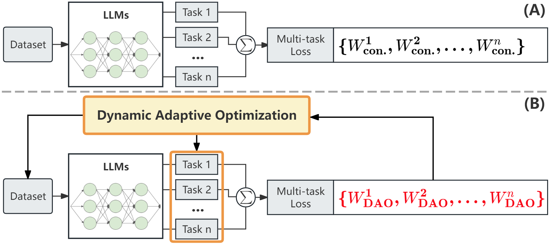
Figure 1: Illustration of the traditional multi-task learning approach with constant weights (A) and our proposed multi-task learning framework with the DAO module (B). In (A), constant weights $\{W^{1}_{\text{con.}},W^{2}_{\text{con.}},\dots,W^{n}_{\text{con.}}\}$ are used to combine the losses of Task 1 to Task $n$. In (B), dynamic adaptive loss adjusts the weights $\{W^{1}_{\text{DAO}},W^{2}_{\text{DAO}},\dots,W^{n}_{\text{DAO}}\}$ dynamically during the training process based on the current batch of data and the losses of different tasks.

Traditionally, sentiment analysis employs various approaches, primarily including machine learning algorithms (e.g., SVM and Naive Bayes (Dang, Moreno-García, and De la Prieta 2020)) and deep learning methods (e.g., CNN and LSTM (Zhang, Wang, and Liu 2018)). Recently, Large Language Models (LLMs) such as BERT (Devlin et al. 2018), GPT (Radford et al. 2018), and RoBERTa (Liu et al. 2019) have revolutionized Natural Language Processing (NLP) by achieving state-of-the-arts performance across various NLP tasks. For instance, Hande et al. (2021) explore multi-task learning for sentiment analysis and offensive language identification, while Ding et al. (2024b) conduct aspect-based sentiment analysis.

However, the conventional approach of fine-tuning these models by assigning constant weights to the loss functions of different tasks in the overall loss function does not always guarantee optimal convergence. This limitation is particularly pronounced when dealing with non-standard datasets or in scenarios with limited data availability (Kendall, Gal, and Cipolla 2018). Consequently, a notable performance gap often emerges between the fine-tuned model and the anticipated performance under ideal conditions.

To address these challenges, we propose a multi-task learning framework with the dynamic adaptive optimization (DAO) module. Specifically, by incorporating multi-task learning (Houlsby et al. 2019), the model can capture more nuanced sentiment patterns even with limited data, facilitating more effective convergence. Additionally, the introduction of the DAO module allows the model to dynamically adjust the weights of different loss functions in each training iteration (see Figure 1). The key component of the DAO module is dynamic adaptive loss, which enables the model to adapt to the evolving learning process and optimize the balance between different tasks, ultimately leading to improved overall performance. The main contributions of this paper are as follows:

• We identify a performance gap in LLMs fine-tuned for sentiment analysis within the financial domain using multi-task learning, particularly when employing constant-loss weights for sub-tasks.

• We design a plug-and-play DAO module that effectively resolves the problem in multi-task learning. The module dynamically adjusts the weights of different tasks based on the relevance and importance of each data batch and the varying difficulty of tasks.

• To reduce the computational overhead of fine-tuning the model, we use LoRA with different parameters to fine-tune the RoBERTa-Large model for the sentiment analysis task without the introduction of inference latency.

• Our framework achieves the best performance, improving Mean Squared Error (MSE) by 15.58% and Accuracy (ACC) by 1.24% compared to previous works.

Motivation

In the sentiment polarity analysis task for exchange rate texts, we observe that the performance of the RoBERTa-Large (Liu et al. 2019) is unsatisfactory after fine-tuning on the standard and customized financial text dataset (Ding et al. 2024a). This can be attributed to the model’s lack of exposure to news domain-specific texts containing specialized jargon, implicit sentiments, and subtle variations. Subsequently, we employ an alternative RoBERTa-Large model, Twitter-RoBERTa-Large (Loureiro et al. 2023) fine-tuned on a tweet news dataset, and the model’s performance shows a slight improvement.

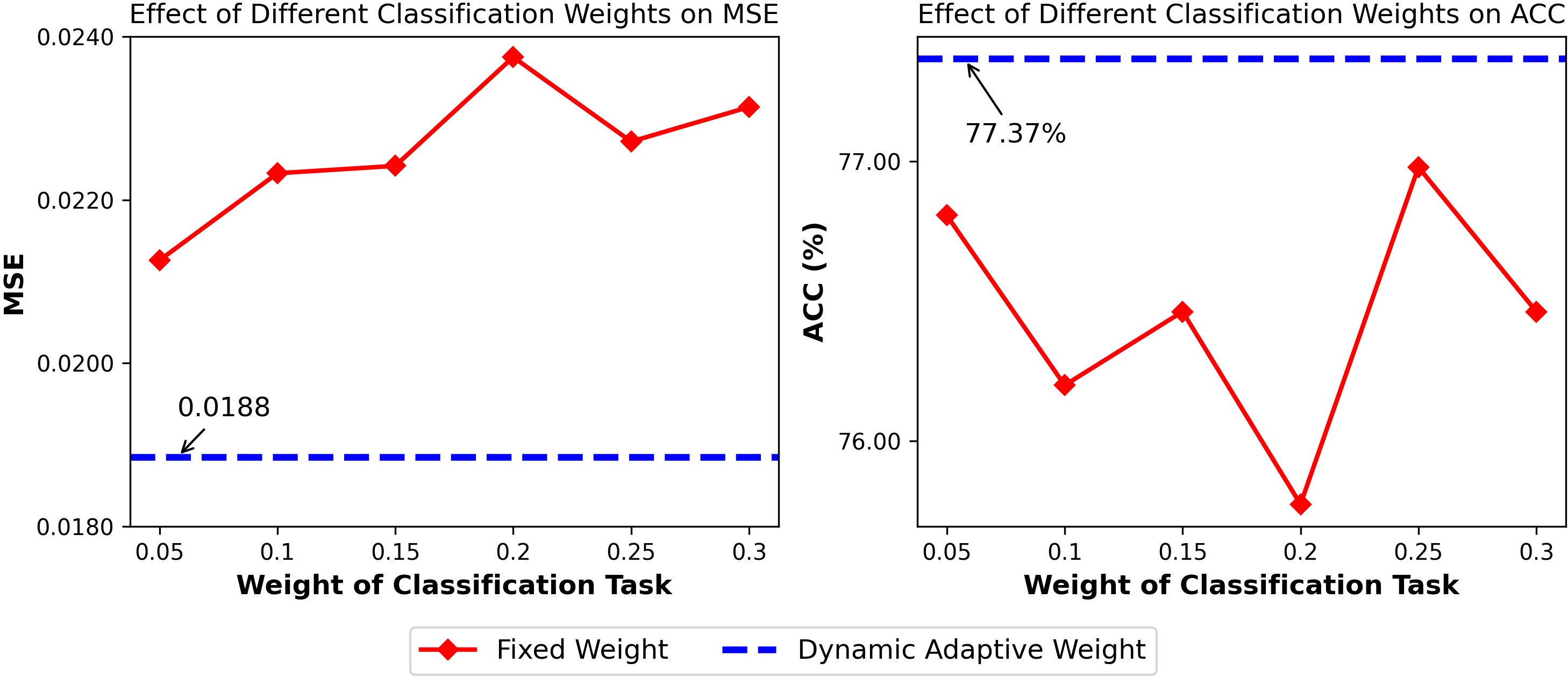
Figure 2: Effect of different classification task weights on MSE and ACC in multi-task learning, compared with the performance of our proposed framework incorporating the DAO module.

In the subsequent multi-task learning experiments, we modulate the weight ($W_{c}$) of the classification task within the total loss function, with the regression task weight correspondingly set to ($1-W_{c}$). Figure 2 illustrates the model’s task performance across different tasks as a result of varying weights. As the weight of the classification task increases, the MSE increases while the ACC decreases, indicating a trade-off between the regression and classification objectives. The optimal balance appears to be around a classification weight of 0.25, where both MSE is relatively low and ACC is relatively high. Upon integration of the DAO, the model achieves superior task performance across all metrics, yielding the lowest MSE of 0.0188 and the highest ACC of 77.37%.

Method

In this section, we will introduce traditional sentiment analysis, our framework incorporating the DAO module with LoRA.

Traditional Sentiment Analysis

Backbone: RoBERTa-Large. In sentiment analysis, LLMs serve as text data embedding generators, concatenating various task-specific heads for various sentiment analysis tasks. This work employs RoBERTa-Large as the embedding generator for text data, as illustrated in Figure 3 (A). The training set is defined as $D=\{(x_{i},y_{i})\}_{i=1}^{N}$, where $N$ denotes the total number of texts, $x_{i}$ represents each text in the dataset, and $y_{i}\in[-1,1]$ corresponds to the annotated sentiment polarity score.

The pre-trained RoBERTa tokenizer $\mathrm{Tokenizer}(\cdot)$ processes each text $x_{i}$ in the dataset, and then the tokenized text passes through 24 Transformer encoder blocks $\text{Encoder}(\cdot)$ to generate the final hidden state $H_{i}$:

$$H_{i}=\mathrm{Encoder}(\mathrm{Tokenizer}(x_{i})),$$ (1)

where $H_{i}\in\mathbb{R}^{1\times 1024}$. This hidden state serves as input to task-specific heads. For sentiment polarity analysis, we implement a regression head (Figure 3 (B)) comprising two linear layers and a sigmoid activation function:

$$S_{i}=\mathrm{LL}_{2}(\sigma(\mathrm{LL}_{1}(H_{i}))),$$ (2)

where $\mathrm{LL}_{1}:\mathbb{R}^{1024}\rightarrow\mathbb{R}^{128}$ is the first linear layer, $\sigma(\cdot)$ denotes the sigmoid function, and $\mathrm{LL}_{2}:\mathbb{R}^{128}\rightarrow\mathbb{R}$ produces the final sentiment polarity score $S_{i}\in[-1,1]$.

For the regression task, we use Mean Squared Error (MSE) as the loss function, denoted as $L_{\mathrm{r}}$:

$$L_{\mathrm{r}}=\frac{1}{n}\sum_{i=1}^{n}(\hat{y}_{i}-y_{i})^{2}$$ (3)

where $n$ denotes the number of texts texts in the training set, $\hat{y}_{i}$ represents the predicted polarity score, and $y_{i}$ is the ground truth sentiment polarity score.

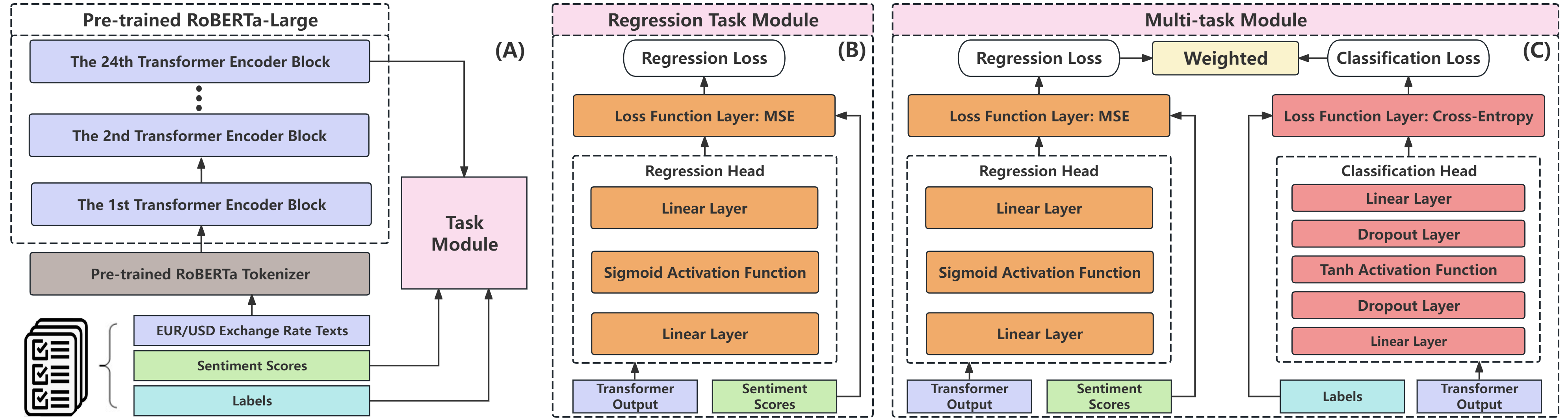
Figure 3: The diagram outlines the application of the pre-trained RoBERTa-Large model for sentiment analysis, segmented into three main parts: (A) RoBERTa-Large as the backbone combined with a task-specific module, (B) a regression task module, and (C) a multi-task module that handles both regression and classification tasks.

Standard Learning. In sentiment analysis, particularly in data-limited scenarios, enhancing model performance is crucial. We introduce a multi-task learning approach. Specifically, we incorporate a classification task alongside the regression task to better capture the sentiment tendencies embedded in the text. This approach mitigates the impact of noise and small fluctuations while effectively alleviating the data sparsity problem often encountered in sentiment analysis. (Saif, He, and Alani 2012; Kim et al. 2013)

Based on empirical observations, we map the continuous sentiment polarity scores to discrete sentiment categories ranging from 0 to 4, representing strong negative, negative, neutral, positive, and strong positive sentiments, respectively. The mapping function is defined as:

$$z_{i}=\begin{cases}4,&\text{if }y_{i}>0.5;\\ 3,&\text{if }0.049<y_{i}\leq 0.5;\\ 2,&\text{if }-0.049\leq y_{i}\leq 0.049;\\ 1,&\text{if }-0.5\leq y_{i}<-0.049;\\ 0,&\text{if }y_{i}<-0.5.\end{cases}$$ (4)

Here, $z_{i}$ denotes the discrete sentiment classification of $x_{i}$. Consequently, we redefine our dataset as $D=\{(x_{i},y_{i},z_{i})\}_{i=1}^{N}$.

For the classification task, we implement a classification head as illustrated in Figure 3 (C). This head comprises two dropout layers, two linear layers, and a Tanh activation function. The process can be formalized as follows:

$$H_{i}^{\prime}=\mathrm{LL}_{1}(\mathrm{DP}_{1}(H_{i})),$$ (5)

where $H_{i}^{\prime}\in\mathbb{R}^{1\times 128}$ is an intermediate representation, $\mathrm{DP}_{1}(\cdot)$ is the first dropout layer for regularization, and $\mathrm{LL}_{1}:\mathbb{R}^{1024}\rightarrow\mathbb{R}^{128}$ is the first linear layer.

The classification label $C_{i}$ for the $i$-th text is then computed as:

$$C_{i}=\mathrm{LL}_{2}(\mathrm{DP}_{2}(\mathrm{Tanh}(H_{i}^{\prime}))),$$ (6)

where $\mathrm{Tanh}(\cdot)$ introduces non-linearity, $\mathrm{DP}_{2}(\cdot)$ is the second dropout layer, and $\mathrm{LL}_{2}:\mathbb{R}^{128}\rightarrow\mathbb{R}^{5}$ maps to the five discrete classification labels.

For the classification task, we use Cross-Entropy (CE) loss to measure the difference between predicted probabilities and actual class labels. The classification loss $L_{\mathrm{c}}$ is formulated as:

$$L_{\mathrm{c}}=-\sum_{i=1}^{n}y_{i}\log(\hat{y}_{i})$$ (7)

where $n$ is the number of texts. $y_{i}$ is the actual class label, and $\hat{y}_{i}$ is the predicted class label.

To jointly optimize the regression and classification tasks, we define a multi-task learning loss $L_{\mathrm{mtl}}$:

$$L_{\mathrm{mtl}}=w_{r}L_{r}+w_{c}L_{c},$$ (8)

where $L_{r}$ and $L_{c}$ are the regression and classification losses, respectively, and $w_{r}$ and $w_{c}$ are hyperparameters that manage the trade-off between the tasks.

Dynamic Adaptive Optimization

In the context of multi-task learning with LLMs, two primary challenges arise: Task-level challenge: inter-task difficulty discrepancy. The loss functions associated with regression and classification tasks may exhibit significant disparities in their magnitudes. Consequently, this discrepancy can lead to the dominance of one task over others during the training process, potentially hindering the model’s ability to effectively learn and generalize across all tasks. Data-level challenge: imbalanced data distribution. Within each training batch, the sample distribution can exhibit considerable variability, and the class distribution may be inherently imbalanced. As a result, the model may be susceptible to overfitting or underfitting for certain classes, compromising its overall performance and generalization capability.

To address these challenges, we propose a DAO module as shown in Figure 4 (A), which is a learnable neural network integrated into the multi-task learning framework.

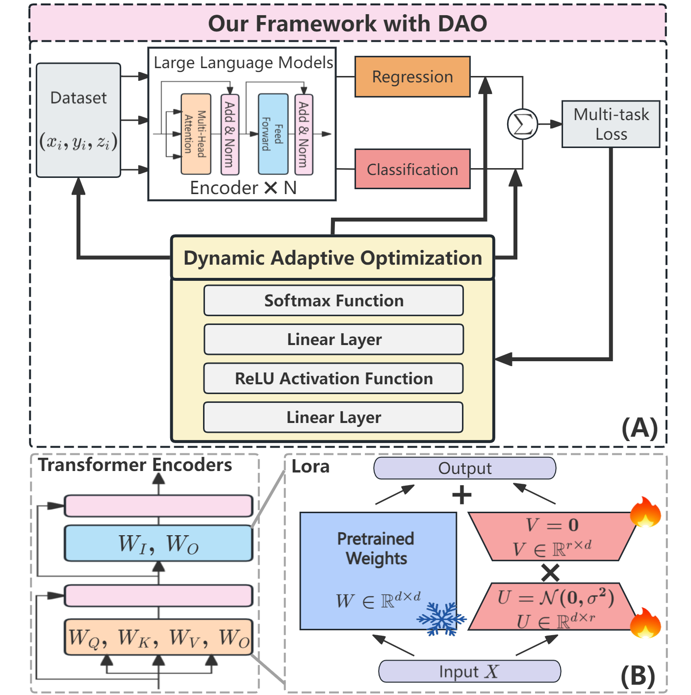
Figure 4: (A) Workflow of the Multi-Task Learning Module with DAO, and (B) Application of LoRA Technique

Solution #1: Inter-task Difficulty Discrepancy. Due to the different magnitudes of the loss functions for regression and classification tasks, directly summing them may cause one task to dominate the entire training process. To balance the contributions of different tasks, we introduce a gradient-based weighting method. Specifically, we define the total multi-task loss function $L^{t}_{\text{mtl}}$ as follows:

$$L^{t}_{\text{mtl}}=\lambda_{r}^{t}w_{r}^{t}L_{r}^{t}+\lambda_{c}^{t}w_{c}^{t}L_{c}^{t},$$ (9)

where $L_{r}^{t}$ and $L_{c}^{t}$ represent the losses of the regression and classification tasks at step $t$, respectively, $w_{r}^{t}$ and $w_{c}^{t}$ are the task-specific weights, and $\lambda_{r}^{t}$ and $\lambda_{c}^{t}$ are the gradient-based weighting coefficients.
At each training step, we compute the gradients of the regression and classification task losses:

$$g_{r}^{t}=\nabla L_{r}^{t},\quad g_{c}^{t}=\nabla L_{c}^{t}.$$ (10)

Then, we use the L2 norms of these gradients to compute the gradient-based weighting coefficients:

$$\lambda_{r}^{t}=\frac{|g_{c}^{t}|}{|g_{r}^{t}|+|g_{c}^{t}|},\quad\lambda_{c}^{t}=\frac{|g_{r}^{t}|}{|g_{r}^{t}|+|g_{c}^{t}|}.$$ (11)

These gradient-based weighting coefficients are used to balance the learning progress of different tasks and scale them to similar magnitudes in the total multi-task loss function $L^{t}_{\text{mtl}}$.

Solution #2: Imbalanced Data Distribution. We introduce a regularization term and class-specific weights into the classification loss function. The regularization term $-\alpha\log p_{k}^{t}$ encourages the model to pay more attention to minority classes with smaller sample proportions, while the class-specific weights $v_{k}^{t}$ are inversely proportional to the sample proportions $p_{k}^{t}$:

$$v_{k}^{t}=\frac{1}{(p_{k}^{t})^{\beta}},$$ (12)

where $\beta$ is a parameter that controls the degree of class balancing.

We use $D$ to denote the entire dataset and $D^{t}$ to represent the batch of data sampled at time step $t$. For each batch $D^{t}$, we calculate the proportion of samples $p_{k}^{t}$ belonging to class $k$ as:

$$p_{k}^{t}=\frac{|D_{k}^{t}|}{|D^{t}|},$$ (13)

where $|D_{k}^{t}|$ and $|D^{t}|$ denote the number of samples in batch $D^{t}$ belonging to class $k$ and the total number of samples in batch $D^{t}$, respectively.

To incorporate the regularization term $-\alpha\log p_{k}^{t}$ and the class-specific weights $v_{k}^{t}$ into the classification loss function, we define the imbalanced data distribution loss $L_{\text{imb}}^{t}$ conditioned on $D^{t}$ as:

$$L_{\text{imb}}^{t}(D^{t})=\sum_{k=1}^{B}v_{k}^{t}(p_{k}^{t}L_{c,k}^{t}-\alpha\log p_{k}^{t}).$$ (14)

This loss captures the sample distribution and class proportions specific to the current batch, allowing the model to dynamically adapt to the characteristics of each batch during training. We then incorporate the imbalanced data distribution loss $L_{\text{imb}}^{t}(D^{t})$ into the total multi-task loss function $L^{t}_{\text{mtl}}$ from Challenge 1, along with the task-specific weights $w_{r}^{t}$ and $w_{c}^{t}$:

$$L_{\text{mtl}}^{t}(D^{t}) =\lambda_{r}^{t}w_{r}^{t}L_{r}^{t}+\lambda_{c}^{t}w_{c}^{t}L_{\text{imb}}^{t}(D^{t})$$

$$=\lambda_{r}^{t}w_{r}^{t}L_{r}^{t}+\lambda_{c}^{t}w_{c}^{t}\sum_{k=1}^{B}v_{k}^{t}(p_{k}^{t}L_{c,k}^{t}-\alpha\log p_{k}^{t}),$$ (15)

where $\lambda_{r}^{t}$ and $\lambda_{c}^{t}$ are the gradient-based weighting coefficients, $v_{k}^{t}$ are the class-specific weights, and $L_{c,k}^{t}$ is the classification loss for class $k$ at time step $t$. The total multi-task loss $L_{\text{mtl}}^{t}$ is now conditioned on the current batch $D^{t}$, allowing the model to adapt to the specific characteristics of each batch during training.

To learn the hyperparameters $\alpha$ and $\beta$, we treat them as learnable parameters of the DAO Module and update them using gradient descent along with the other parameters of the module. During the backward pass, the gradients of the DAO Module loss $L_{\text{mtl}}^{t}(D^{t})$ with respect to $\alpha$ and $\beta$ are computed as follows:

$$\frac{\partial L_{\text{mtl}}^{t}(D^{t})}{\partial\alpha}=-\lambda_{c}^{t}w_{c}^{t}\sum_{k=1}^{B}v_{k}^{t}\log p_{k}^{t}.$$ (16)

To compute the gradient with respect to $\beta$, we apply the chain rule and substitute the expression for $\frac{\partial v_{k}^{t}}{\partial\beta}$:

$$\frac{\partial L_{\text{mtl}}^{t}(D^{t})}{\partial\beta} =-\lambda_{c}^{t}w_{c}^{t}\sum_{k=1}^{B}\frac{\partial v_{k}^{t}}{\partial\beta}(p_{k}^{t}L_{c,k}^{t}-\alpha\log p_{k}^{t})$$

$$=\lambda_{c}^{t}w_{c}^{t}\sum_{k=1}^{B}\frac{\log p_{k}^{t}}{(p_{k}^{t})^{\beta}}(p_{k}^{t}L_{c,k}^{t}-\alpha\log p_{k}^{t}).$$ (17)

The hyperparameters $\alpha$ and $\beta$ are then updated using an optimizer such as Adam or AdamW.

To obtain the task-specific weights $w_{r}^{t}$ and $w_{c}^{t}$, we pass the gradient-weighted regression loss $\lambda_{r}^{t}L_{r}^{t}$, the gradient-weighted imbalanced data distribution loss $\lambda_{c}^{t}L_{\text{imb}}^{t}(D^{t})$, and the current batch $D^{t}$ through the DAO Module:

$$w_{r}^{t},w_{c}^{t}=\text{DAO}(\lambda_{r}^{t}L_{r}^{t},\lambda_{c}^{t}L_{\text{imb}}^{t}(D^{t}),D^{t})$$ (18)

Specifically, we first concatenate these weighted losses and map them to a hidden space through a fully connected layer (FC₁) followed by a ReLU activation function:

$$\mathbf{h}^{t} =\text{ReLU}(\text{FC}_{1}([\lambda_{r}^{t}L_{r}^{t},\lambda_{c}^{t}L_{\text{imb}}^{t}(D^{t})]))$$

$$=\text{ReLU}(\text{FC}_{1}([\lambda_{r}^{t}L_{r}^{t},\lambda_{c}^{t}\sum_{k=1}^{B}v_{k}^{t}(p_{k}^{t}L_{c,k}^{t}-\alpha\log p_{k}^{t})])).$$ (19)

The hidden representation $\mathbf{h}^{t}$ encodes the information from the weighted losses and the current batch data. Next, we use another fully connected layer (FC₂) to map the hidden representation $\mathbf{h}^{t}$ to a two-dimensional vector $\mathbf{s}^{t}$:

$$\mathbf{s}^{t}=\text{FC}_{2}(\mathbf{h}^{t}).$$ (20)

Finally, we pass the vector $\mathbf{s}^{t}$ through a Softmax function to obtain the task-specific weights $w_{r}^{t}$ and $w_{c}^{t}$ based on the current batch $D^{t}$:

$$[w_{r}^{t},w_{c}^{t}]=\text{Softmax}(\mathbf{s}^{t}).$$ (21)

In summary, the DAO Module receives batch-level information including losses, gradients, sample distributions, and the current batch $D^{t}$. The DAO module dynamically adjusts the weights, allowing the model to adapt to the characteristics of different batches, balance the learning progress of tasks, and mitigate the data imbalance problem. The gradient-based weighting coefficients $\lambda_{r}^{t}$ and $\lambda_{c}^{t}$ help address the inter-task difficulty discrepancy, while the learnable hyperparameters $\alpha$ and $\beta$ are directly related to the imbalanced data distribution and are optimized using gradient descent to minimize the multi-task learning loss $L_{\text{mtl}}^{t}$.

LoRA

We implement LoRA (Hu et al. 2021) for parameter-efficient fine-tuning (PEFT) of the pre-trained RoBERTa-large model. LoRA injects trainable low-rank decomposition matrices into each layer, reducing parameters while maintaining performance.

LoRA introduces rank-$r$ matrices $U\in\mathbb{R}^{d\times r}$ and $V\in\mathbb{R}^{r\times d}$ into each attention block and feed-forward network, as shown in Figure 4 (B). The figure illustrates how LoRA is integrated into the Transformer encoder, with pretrained weights $W$ remaining frozen while low-rank matrices are trained. The adjusted weight matrix $W^{\prime}$ during forward propagation is:

$$f(x)=(W+UV)\cdot X+b,$$ (22)

where $b$ is the bias, and $X$ is the input as illustrated in Figure 4 (B). Only $U$ and $V$ are updated during training, significantly reducing trainable parameters and potentially accelerating training.

In traditional multi-task learning with constant weight, this approach can lead to suboptimal performance. Our proposed framework incorporates the DAO module that dynamically adjusts task weights based on their relative importance, gradients, and data characteristics during training. This batch-level dynamic adaptive loss addresses the limitations of constant-weight approaches by considering the varying difficulties and contributions of each task and the characteristics of the data in each batch. The plug-and-play nature of the DAO module allows for flexible integration into various multi-task learning scenarios, making it applicable to a wide range of tasks.

Evaluation

Software and Hardware

We use Ubuntu 22.04, Python 3.9.19, PyTorch 2.3.1, PEFT 0.12.0, and CUDA 12.4, running on a system with 32GB RAM and an NVIDIA RTX 3090 Ti GPU with 24GB VRAM.

Setup and Dataset

Benchmark. We use diffrent benchmarks to verify our framework. We establish three benchmark: RoBERTa-Large (Liu et al. 2019) for regression, Twitter-RoBERTa-Large (Loureiro et al. 2023) for regression, and Twitter-RoBERTa-Large with constant-weight multi-task learning for regression and classification. Additionally, we propose two methods: Twitter-RoBERTa-Large with DAO for multi-task learning, and the multi-task learning framework using Twitter-RoBERTa-Large with DAO and LoRA.

Epoch	RoBERTa-Large for Regression					Twitter-RoBERTa-Large for Regression
	MSE	MAE	RMSE	$R^{2}$ (%)	GPU	MSE	MAE	RMSE	$R^{2}$ (%)	GPU
20	0.019064	0.098594	0.138074	78.59	21,780	0.021369	0.106370	0.146183	76.00	21,780
40	0.019805	0.099945	0.140731	77.76	MiB	0.019398	0.100493	0.139277	78.21	MiB
60	0.018328	0.096009	0.135719	78.86	Time	0.019353	0.099428	0.139116	78.27	Time
80	0.018299	0.095898	0.137581	78.74	130,525	0.018617	0.097000	0.136446	79.09	130,553
100	0.018949	0.095773	0.137657	78.72	seconds	0.018714	0.097313	0.136801	78.98	seconds

Table 1: Performance Metrics of Single Task Experiments.

Epoch	Multi-Task Learning with constant Weight					Multi-Task Learning with DAO
	MSE	ACC	Precision	F1	GPU	MSE	ACC	Precision	F1	GPU
20	0.022544	74.83	76.37	75.39	21,780	0.018983	75.60	76.99	75.99	22,336
40	0.022930	75.90	76.39	76.01	MiB	0.018668	76.64	77.92	76.83	MiB
60	0.023744	75.52	75.94	75.61	Time	0.018841	76.68	78.06	76.94	Time
80	0.022612	76.08	75.97	75.88	129,959	0.019000	76.89	77.98	77.00	211,024
100	0.022326	76.11	76.17	76.05	seconds	0.018848	77.06	78.28	77.37	seconds

Table 2: Performance Metrics of Multi-Task Learning Experiments.

Epoch	LoRA (Rank = 128)					LoRA (Rank = 256)
	MSE	ACC	Precision	F1	Resource	MSE	ACC	Precision	F1	Resource
20	0.020855	75.13	76.73	75.56	22,852	0.020905	75.13	77.44	75.78	24,224
40	0.020442	75.13	77.25	75.80	MiB	0.019155	76.72	78.46	77.00	MiB
60	0.019320	76.55	78.10	76.93	———	0.019064	76.42	78.39	76.87	———
80	0.019026	76.25	77.93	76.65	247,452	0.018804	75.82	77.84	76.25	266,674
100	0.019057	76.33	78.02	76.76	seconds	0.018747	76.03	78.03	76.47	seconds
Epoch	LoRA (Rank = 384)					LoRA (Rank = 512)
20	0.020939	75.17	76.82	75.76	19,550	0.020835	75.00	76.68	75.66	22,336
40	0.019411	75.09	76.94	75.52	MiB	0.018324	76.85	78.27	76.97	MiB
60	0.018673	75.73	77.52	76.14	———	0.018376	76.12	77.74	76.31	———
80	0.018651	75.39	77.03	75.69	286,793	0.018580	76.76	77.67	76.65	324,013
100	0.018610	75.47	77.04	75.68	seconds	0.018571	76.38	77.40	76.35	seconds

Table 3: Performance Metrics of LoRA at Different Ranks.

Evaluation Metrics. For the regression task, we utilize MSE, Mean Absolute Error (MAE), Root Mean Squared Error (RMSE), and the Coefficient of Determination ($R^{2}$). For the classification task, we use ACC, weighted Precision, and weighted F1 score.

Dataset. We use a standard and customized financial text dataset that comprises 23,242 preprocessed news and analysis texts on EUR/USD exchange rates (Ding et al. 2024a). This dataset is randomly split into training and validation sets with a 9:1 ratio, and all experiments utilize these two identical datasets. Further information and supplementary details can be found in the Appendix.

Main Results

In this section, we will first introduce the hyperparameters and then analyze the experimental results.

Model Hyperparameters. The training texts exceeding 512 tokens are truncated to the first 512 tokens. The model is trained with a batch size of 10 for 100 epochs, using the AdamW optimizer with a learning rate of 1e-5 and an epsilon value of 1e-8. The training process incorporates 1e2 warmup steps and implements cosine decay for learning rate scheduling. To ensure the reproducibility of the experiments, we set constant random seeds for Python (42), NumPy (42), and PyTorch (42) across all runs.

DAO Module Hyperparameters. The optimizer is Adam with a learning rate of 0.001.

LoRA Parameters. Different LoRA configurations are applied in the experiments, with the rank values set to 8, 16, 32, 64, 128, 256, 384, and 512. Correspondingly, the scaling factor (alpha) for the LoRA matrices is set to one times the rank. The dropout rate for all LoRA configurations is constant at 0.05 to prevent overfitting.

Results. Table 1 presents the performance metrics of RoBERTa-Large and Twitter-RoBERTa-Large on the task of sentiment polarity regression. After 100 epochs of training, RoBERTa-Large achieves an MSE of 0.018949, MAE of 0.095773, RMSE of 0.137657, and $R^{2}$ of 78.72%, while Twitter-RoBERTa-Large demonstrates a 1.24% improvement in MSE, a 1.61% increase in MAE, a 0.62% improvement in RMSE, and a 0.26% increase in $R^{2}$.

These results indicate that Twitter-RoBERTa-Large outperforms RoBERTa-Large, likely due to its fine-tuning on a tweet news dataset, which is more similar to the target domain of financial news compared to the general domain pre-training of RoBERTa-Large. Although there is an improvement in performance, there is still a gap between the current results and the ideal performance. Therefore, a new framework may be necessary to better understand and analyze sentiment in the financial domain.

Table 2 compares the performance of Twitter-RoBERTa-Large using multi-task learning with a constant weight of 0.1 for the classification task and 0.9 for the regression task, and our proposed framework with the DAO module. After 100 epochs of training, the proposed method achieves an MSE of 0.018848, an ACC of 77.06%, a Precision of 78.28%, and an F1 score of 77.37%. Compared to the constant-weight method, the DAO module yields a 15.58% improvement in MSE, a 1.25% improvement in ACC, a 2.77% improvement in Precision, and a 1.74% improvement in F1 score.

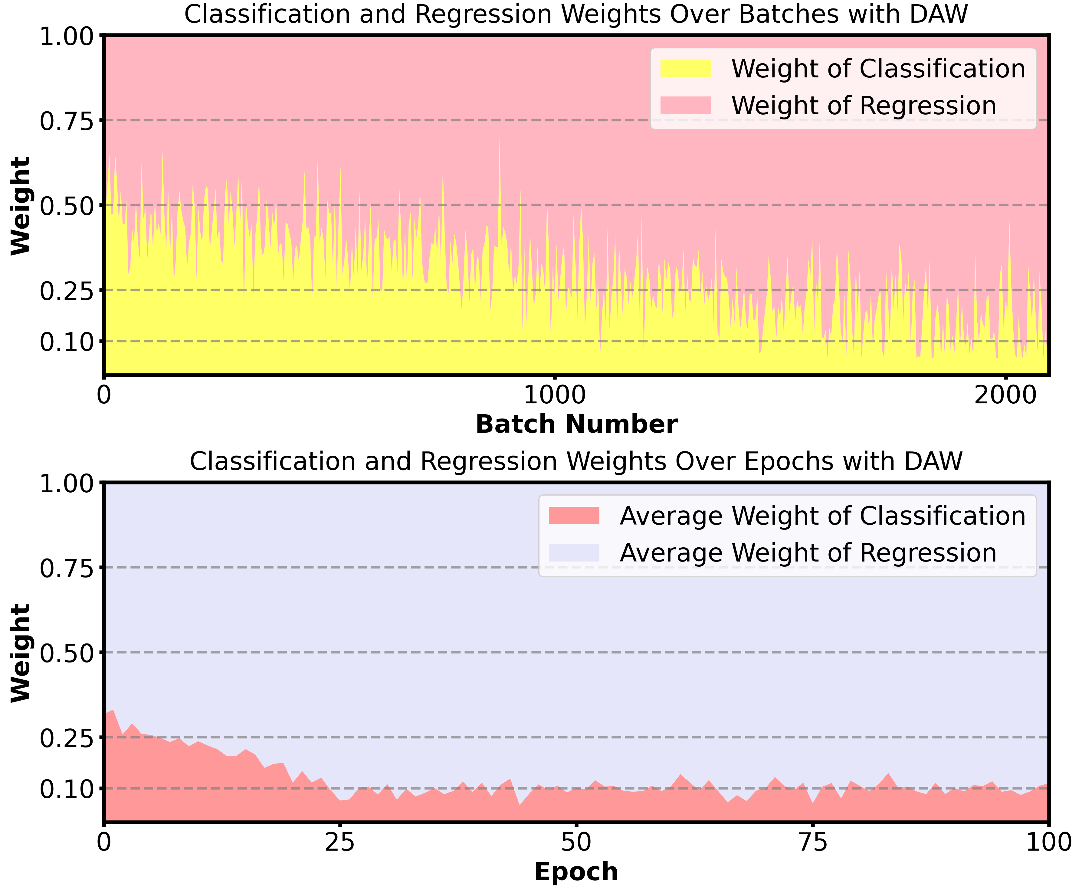
Figure 5: Dynamic adjustment of task weights by the DAO module.

Figure 5 illustrates the changes in the dynamic adaptive loss function during model training, with the weights of the classification and regression tasks set to 1. The upper plot shows the dynamic adjustment of task weights during training. The initial weight of the classification task appears at approximately 0.5 and exhibits an oscillating decrease, stabilizing around 0.15 after approximately 1600 batches. The lower plot displays the average weights of the classification and regression tasks throughout the entire training process. The average weight of the classification task gradually decreases from about 0.3 to 0.1 over the first 25 epochs and continues to fluctuate around 0.1 for the remainder of the training.

Additionally, significant differences in the loss function values for the two tasks are observed throughout the training process, with the discrepancy consistently remaining within at least one order of magnitude. When using the DAO module, the loss function accelerates the convergence of model training. Compared to the constant-weight loss function with a weight of 0.1, the loss function value significantly decreases within the first 50 epochs (see subsection Multi-task Loss in Appendix).

These observations demonstrate the DAO module’s effectiveness in adjusting task weights based on relative difficulty and gradients, assigning higher weight to the more challenging regression task and lower weight to the easier classification task. This dynamic adjustment balances the learning progress of both tasks, optimizing overall performance, unlike constant-weight methods that may fail to capture changes in task importance and data characteristics.

Ablation Studies

We ablate our method with DAO using different LoRA ranks, as shown in Table 3, which presents several intriguing observations. Increasing the rank consistently decreases MSE while improving ACC, Precision, and F1 score, suggesting that more trainable parameters enhance model performance. Table 4 illustrates that at a rank of 256, we achieve results comparable to a fully fine-tuned (FF) model with only 80.88% of the FF time. Using the same amount of time, MSE is slightly improved. At a rank of 384, the optimal performance is achieved in 53.00% of the FF time. When the rank increases to 512, we obtain results comparable to the FF model with only 36.85% of the FF time, and the optimal performance is obtained in 66.02% of the time, with MSE improving by 3.68% and ACC improving by 0.12%. Due to CUDA out of memory issues, the batch size was set to 7 in the experiment with a rank of 384, and to 10 in the experiment with a rank of 512.

Rank	Epoch	MSE	ACC	Time	Usage
256	64	0.018838	76.16	170,671 s	80.88%
256	79	0.018665	75.82	210,672 s	99.83%
384	39	0.018434	75.69	111,849 s	53.00%
512	23	0.018730	76.38	77,763 s	36.85%
512	42	0.018154	77.15	139,326 s	66.02%

Table 4: Best Performance Metrics of LoRA at Different Ranks.

The tables in the LoRA subsection of the Appendix illustrate the performance of LoRA fine-tuning across various ranks. The data indicate that higher ranks contribute to enhanced model performance, demonstrating that an increase in rank positively influences outcomes. The corresponding line charts reveal that as the number of epochs increases, both MSE and ACC initially decrease, reaching optimal performance, before subsequently rising again. This pattern suggests that while the model’s generalization ability improves with training, the limited parameter count leads to a deterioration in metrics beyond a certain number of epochs, indicative of overfitting.

These results underscore the effectiveness of LoRA in reducing fine-tuning computational costs while maintaining performance, with a trade-off between enhanced performance and increased parameter count and training time at higher ranks.

Related Work

LLMs NLP advancements lead to the widespread application of LLMs in sentiment analysis tasks. ChatGPT shows significant potential in automating student feedback analysis, outperforming traditional deep learning models (Shaikh et al. 2023). Pre-trained models like BERT achieve state-of-the-arts results by learning contextual word representations (Liao et al. 2021). In Arabic sentiment analysis, transformer-based models like RoBERTa and XLNet push boundaries despite language complexities (Alduailej and Alothaim 2022). Krugmann and Hartmann (2024) reveals that GPT-3.5, GPT-4, and Llama 2 can compete with and sometimes surpass traditional transfer learning methods in sentiment analysis. Carneros-Prado et al. (2023) highlights the versatility of pre-trained LLMs like GPT-3.5 in diverse NLP applications, including emotion recognition. However, fully fine-tuning these LLMs for specific tasks remains computationally expensive and time-consuming, posing challenges for both academia and industry.

PEFT To address computational challenges, researchers introduce PEFT methods for LLMs. Hu et al. (2023) presents LLM-Adapters, integrating adapters into LLMs and achieving comparable performance to powerful 175B parameter models using only 7B parameters in zero-shot tasks. Lei et al. (2023) introduces Conditional Adapters (CODA), which adds sparse activation and new parameters to pre-trained models for efficient knowledge transfer, significantly speeding up inference. Hu et al. (2021) proposes LoRA, which injects trainable low-rank decomposition matrices into each Transformer layer, reducing parameters while maintaining performance on par with full fine-tuning.

Conclusion

In this work, we propose a multi-task learning framework with a DAO module for LLM-based sentiment analysis. The DAO module dynamically adjusts task weights based on their relative importance and data characteristics, addressing inter-task difficulty and data imbalance issues. This plug-and-play module can be seamlessly integrated into existing models, enhancing their adaptability to diverse tasks and datasets. Combined with LoRA for efficient fine-tuning, our approach achieves state-of-the-art performance in financial sentiment analysis, significantly improving MSE and accuracy over previous methods.

In the future work, we will explore the use of data-aware classification tasks to enhance the performance of multi-task learning with DAO module under data-limited scenarios.

Appendix A Appendix

Dataset

In this work, the text dataset comes from another study (Ding et al. 2024a). Specifically, the dataset is collected from investing.com and forexempire.com, focusing on the EUR/USD exchange rate. The dataset spans from February 6, 2016, to January 19, 2024, encompassing all accessible data on these platforms, resulting in a total of 35,427 records. To address the presence of noise and information irrelevant to the target exchange rate, we use ChatGPT-4.0 and prompt engineering techniques to filter the raw dataset. Further analysis reveals that typically only individual paragraphs or multiple sentences within articles directly relate to the EUR/USD exchange rate, likely catering to readers’ diverse interests. To extract the most relevant parts and refine the dataset, we process the text data using ChatGPT-4.0, yielding a final text dataset comprising 23,242 records.

Sentiment polarity annotation in exchange rate texts is particularly complex because such texts are often filled with professional terminology, implied emotions related to market conditions, and subtle variations across industries. Moreover, as exchange rate issues involve two countries, significant positive or negative news about one country can have a substantial impact on financial markets. For example, a large amount of positive news about the United States may strengthen the US dollar, typically leading to a decrease in the EUR/USD exchange rate, while negative news may result in the opposite effect. However, news texts often contain information about both countries simultaneously, making accurate classification of the text complex, with news from the two countries exhibiting a zero-sum effect in sentiment analysis.

To address this challenge, we leverage LLMs to annotate the text with sentiment polarity scores. Large language models have advantages in understanding long text dependencies, complex semantics, and processing high-noise text. For this purpose, we use ChatGPT-4.0 integrated with carefully designed and iteratively refined prompts to annotate the training dataset. To guard against potential and unidentified errors, the model is also required to provide reasons for its assigned sentiment scores. In our prompt engineering, we define the sentiment score range as [-1, 1], with scores close to 1 indicating strong positive sentiment and vice versa. Scores near zero represent neutral sentiment, ensuring comprehensive coverage of the subtle emotional details present in financial narratives.

Evaluation Metrics

For the sentiment score regression task, where the model predicts a continuous sentiment polarity score, we employ the following metrics:

• Mean Squared Error (MSE) calculates the average squared differences between the predicted sentiment polarity scores ($\hat{y}_{i}$) and the annotated sentiment polarity scores ($y_{i}$) in the test set. MSE provides a measure of the model’s accuracy in predicting the exact sentiment scores. It is defined as:

  $$\text{MSE}=\frac{1}{n}\sum_{i=1}^{n}(y_{i}-\hat{y}_{i})^{2}$$

  where $n$ is the number of texts in the test set.

• Mean Absolute Error (MAE) measures the average magnitude of the absolute errors between the predicted and annotated sentiment polarity scores, ignoring their direction. MAE helps in understanding the average error magnitude and is less sensitive to outliers compared to MSE. It is formulated as:

  $$\text{MAE}=\frac{1}{n}\sum_{i=1}^{n}\left|y_{i}-\hat{y}_{i}\right|$$

• Root Mean Squared Error (RMSE) is the square root of MSE and provides the error magnitude in the same units as the sentiment polarity scores. RMSE is more interpretable than MSE and is calculated as:

  $$\text{RMSE}=\sqrt{\text{MSE}}$$

• R-squared (R²) indicates the proportion of variance in the sentiment polarity scores that can be explained by the model’s predictions. It provides a measure of how well the model fits the data, with values closer to 1 indicating a better fit. R-squared is defined as:

  $$R^{2}=1-\frac{\sum_{i=1}^{n}(y_{i}-\hat{y}_{i})^{2}}{\sum_{i=1}^{n}(y_{i}-\bar{y})^{2}}$$

  where $\bar{y}$ represents the mean of the annotated sentiment polarity scores in the test set.

For the sentiment classification task, where texts are categorized into five sentiment classes (e.g., strong positive, positive, neutral, negative, strong negative), we calculate the following metrics:

• Accuracy (ACC): the ratio of correctly predicted sentiment classes to the total number of predictions. It measures the overall correctness of the model’s classifications and is defined as:

  $$\text{ACC}=\frac{\sum_{i=1}^{5}TP_{i}}{\sum_{i=1}^{5}(TP_{i}+FN_{i})}$$

  where $TP_{i}$ is the number of instances correctly predicted as class $i$, and $FN_{i}$ is the number of instances that actually belong to class $i$ but are wrongly predicted as other classes.

• Precision: the ratio of correctly predicted positive instances to all instances predicted as positive. It measures the model’s ability to avoid false positives and is calculated as:

  $$\text{Precision}=\frac{TP_{pos}}{TP_{pos}+FP_{pos}}$$

  where $TP_{pos}$ is the number of positive instances correctly predicted as positive, and $FP_{pos}$ is the number of non-positive instances wrongly predicted as positive.

• Recall (or Sensitivity): the ratio of correctly predicted positive instances to all actual positive instances. It measures the model’s ability to identify all positive instances and is calculated as:

  $$\text{Recall}=\frac{TP_{pos}}{TP_{pos}+FN_{pos}}$$

  where $FN_{pos}$ is the number of positive instances wrongly predicted as non-positive.

• F1 Score: the harmonic mean of Precision and Recall, providing a balanced measure of the model’s performance, especially when the sentiment classes are imbalanced. It is calculated as:

  $$F1=2\times\frac{\text{Precision}\times\text{Recall}}{\text{Precision}+\text{Recall}}$$

Proof of Equivalence Between Weighted Recall and Accuracy in Multi-Class Classification

In a multi-class classification problem with $n$ classes, let $TP_{i}$, $FN_{i}$, and $\text{Support}_{i}$ denote the true positives, false negatives, and total instances (support) for class $i$, respectively. The recall for class $i$ is given by:

$$\text{Recall}_{i}=\frac{TP_{i}}{TP_{i}+FN_{i}}=\frac{TP_{i}}{\text{Support}_{i}}$$

The weighted recall is then calculated as:

$$\text{Weighted Recall}=\frac{\sum_{i=1}^{n}\text{Recall}_{i}\times\text{Support}_{i}}{\sum_{i=1}^{n}\text{Support}_{i}}$$

Substituting the expression for $\text{Recall}_{i}$:

$$\text{Weighted Recall}=\frac{\sum_{i=1}^{n}\frac{TP_{i}}{\text{Support}_{i}}\times\text{Support}_{i}}{\sum_{i=1}^{n}\text{Support}_{i}}$$

The $\text{Support}_{i}$ terms in the numerator and denominator cancel out, leaving:

$$\text{Weighted Recall}=\frac{\sum_{i=1}^{n}TP_{i}}{\sum_{i=1}^{n}\text{Support}_{i}}$$

This is exactly the formula for overall accuracy:

$$\text{Accuracy}=\frac{TP_{1}+TP_{2}+\ldots+TP_{n}}{\text{Support}_{1}+\text{Support}_{2}+\ldots+\text{Support}_{n}}$$

Therefore, in a multi-class classification setting, weighted recall is mathematically equivalent to accuracy.

Multi-task Loss

Figure 6: Comparison between constant-weight loss and DAO loss

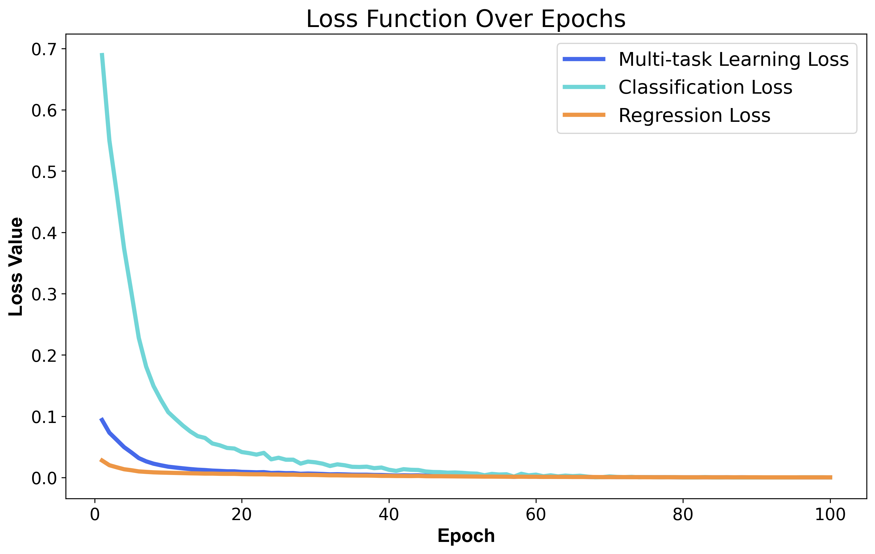
Figure 7: Constant-weight loss

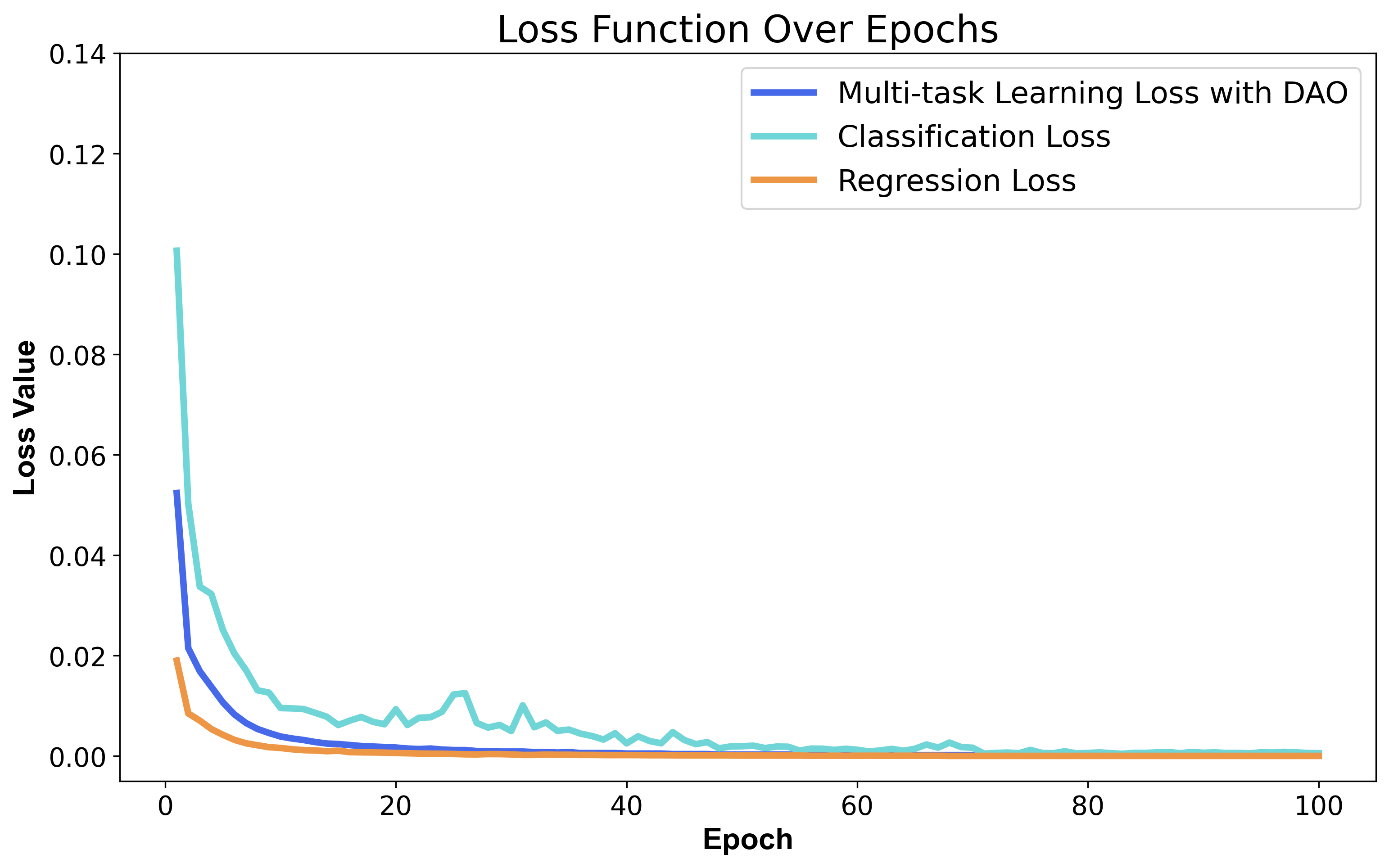
Figure 8: DAO loss

LoRA

Epoch	MSE	MAE	RMSE	R2 (%)	ACC (%)	Pre. (%)	Recall (%)	F1 (%)	GPU
20	0.022544	0.105743	0.150147	74.68	74.83	76.37	74.83	75.39	21,780
40	0.022930	0.107780	0.151428	74.25	75.90	76.39	75.90	76.01	MiB
60	0.023744	0.107770	0.154089	73.33	75.52	75.94	75.52	75.61	Time
80	0.022612	0.104911	0.150373	74.61	76.08	75.97	76.08	75.88	129,959
100	0.022326	0.104055	0.149420	74.93	76.11	76.17	76.11	76.05	seconds

Table 5: Performance Metrics of Multi-Task Learning with constant Weight.

Epoch	MSE	MAE	RMSE	R2 (%)	ACC (%)	Pre. (%)	Recall (%)	F1 (%)	GPU
20	0.018983	0.099503	0.137889	78.65	75.60	76.99	75.60	75.99	22,336
40	0.018668	0.097774	0.136370	79.11	76.64	77.92	76.64	76.83	MiB
60	0.018841	0.094788	0.134705	79.62	76.68	78.06	76.68	76.94	Time
80	0.019000	0.094113	0.133954	79.85	76.89	77.98	76.89	77.00	211,024
100	0.018848	0.093999	0.133965	79.85	77.06	78.28	77.06	77.37	seconds

Table 6: Performance Metrics of Multi-Task Learning with DAO.

Epoch	MSE	MAE	RMSE	R2 (%)	ACC (%)	Pre. (%)	Recall (%)	F1 (%)	GPU
20	0.020452	0.105012	0.143009	77.03	74.18	77.08	74.18	74.99	21,872
40	0.021576	0.104977	0.146887	75.77	73.97	76.17	73.97	74.47	MiB
60	0.022072	0.105496	0.148566	75.21	74.61	76.19	74.61	74.97	Time
80	0.022299	0.106003	0.149330	74.96	74.01	76.20	74.01	74.65	229,915
100	0.022443	0.106440	0.149811	74.80	74.23	76.46	74.23	74.93	seconds

Table 7: Performance Metrics of Multi-Task Learning with DAO Using LoRA with Rank 8.

Epoch	MSE	MAE	RMSE	R2 (%)	ACC (%)	Pre. (%)	Recall (%)	F1 (%)	GPU
20	0.023188	0.111574	0.152275	73.96	73.06	76.55	73.06	74.32	22,248
40	0.023726	0.110474	0.154032	73.35	73.67	75.84	73.67	74.45	MiB
60	0.023067	0.108082	0.151877	74.10	73.41	75.51	73.41	73.96	Time
80	0.022849	0.108018	0.151159	74.34	73.58	75.48	73.58	74.14	234,485
100	0.022653	0.107673	0.150508	74.56	74.14	75.80	74.14	74.63	seconds

Table 8: Performance Metrics of Multi-Task Learning with DAO Using LoRA with Rank 16.

Epoch	MSE	MAE	RMSE	R2 (%)	ACC (%)	Pre. (%)	Recall (%)	F1 (%)	GPU
20	0.022356	0.107567	0.149518	74.89	73.36	76.56	73.36	74.38	22,248
40	0.022449	0.107912	0.149831	74.79	74.61	77.02	74.61	75.49	MiB
60	0.021086	0.103995	0.145209	76.32	74.01	76.20	74.01	74.72	Time
80	0.020559	0.102930	0.143382	76.91	74.61	76.27	74.61	75.08	234,405
100	0.020758	0.103383	0.144078	76.69	74.66	76.44	74.66	75.23	seconds

Table 9: Performance Metrics of Multi-Task Learning with DAO Using LoRA with Rank 32.

Epoch	MSE	MAE	RMSE	R2 (%)	ACC (%)	Pre. (%)	Recall (%)	F1 (%)	GPU
20	0.021734	0.106654	0.147425	75.59	74.27	76.28	74.27	74.97	22,248
40	0.020599	0.102518	0.143523	76.87	74.40	75.99	74.40	74.69	MiB
60	0.020051	0.101035	0.141602	77.48	75.04	76.95	75.04	75.62	Time
80	0.019859	0.100704	0.140922	77.70	74.70	76.45	74.70	75.27	234,230
100	0.019768	0.100669	0.140598	77.80	74.87	76.83	74.87	75.51	seconds

Table 10: Performance Metrics of Multi-Task Learning with DAO Using LoRA with Rank 64.

Epoch	MSE	MAE	RMSE	R2 (%)	ACC (%)	Pre. (%)	Recall (%)	F1 (%)	GPU
20	0.020855	0.103128	0.144412	76.58	75.13	76.73	75.13	75.56	22,852
40	0.020442	0.102753	0.142975	77.04	75.13	77.25	75.13	75.80	MiB
60	0.019320	0.099492	0.138995	78.30	76.55	78.10	76.55	76.93	Time
80	0.019026	0.098734	0.137935	78.63	76.25	77.93	76.25	76.65	247,452
100	0.019057	0.098797	0.138049	78.60	76.33	78.02	76.33	76.76	seconds

Table 11: Performance Metrics of Multi-Task Learning with DAO Using LoRA with Rank 128.

Epoch	MSE	MAE	RMSE	R2 (%)	ACC (%)	Pre. (%)	Recall (%)	F1 (%)	GPU
20	0.020905	0.103332	0.144585	76.52	75.13	77.44	75.13	75.78	24,224
40	0.019155	0.098854	0.138400	78.49	76.72	78.46	76.72	77.00	MiB
60	0.019064	0.098707	0.138074	78.59	76.42	78.39	76.42	76.87	Time
80	0.018804	0.098018	0.137127	78.88	75.82	77.84	75.82	76.25	266,674
100	0.018747	0.097745	0.136919	78.95	76.03	78.03	76.03	76.47	seconds

Table 12: Performance Metrics of Multi-Task Learning with DAO Using LoRA with Rank 256.

Epoch	MSE	MAE	RMSE	R2 (%)	ACC (%)	Pre. (%)	Recall (%)	F1 (%)	GPU
20	0.020939	0.103973	0.144705	76.48	75.17	76.82	75.17	75.76	19,550
40	0.019411	0.100529	0.139324	78.20	75.09	76.94	75.09	75.52	MiB
60	0.018673	0.097442	0.136649	79.03	75.73	77.52	75.73	76.14	Time
80	0.018651	0.097285	0.136570	79.05	75.39	77.03	75.39	75.69	286,793
100	0.018610	0.097076	0.136419	79.10	75.47	77.04	75.47	75.68	seconds

Table 13: Performance Metrics of Multi-Task Learning with DAO Using LoRA with Rank 384.

Epoch	MSE	MAE	RMSE	R2 (%)	ACC (%)	Pre. (%)	Recall (%)	F1 (%)	GPU
20	0.020835	0.103436	0.144345	76.60	75.00	76.68	75.00	75.66	22,336
40	0.018324	0.096110	0.135365	79.42	76.85	78.27	76.85	76.97	MiB
60	0.018376	0.095549	0.135560	79.36	76.12	77.74	76.12	76.31	Time
80	0.018580	0.095503	0.136307	79.13	76.76	77.67	76.76	76.65	324,013
100	0.018571	0.095562	0.136276	79.14	76.38	77.40	76.38	76.35	seconds

Table 14: Performance Metrics of Multi-Task Learning with DAO Using LoRA with Rank 512.

Multi-task Learning with constant Weights

Epoch	MSE	MAE	RMSE	R2 (%)	ACC (%)	Pre. (%)	Recall (%)	F1 (%)	GPU
20	0.020224	0.101586	0.142211	77.29	77.15	76.25	77.15	76.39	21,780
40	0.021843	0.103883	0.147792	75.47	76.72	76.12	76.72	76.31	MiB
60	0.021938	0.103734	0.148115	75.36	76.29	75.92	76.29	75.83	Time
80	0.021660	0.101345	0.147174	75.67	76.85	76.19	76.85	76.33	129,943
100	0.021260	0.100958	0.145807	76.12	76.81	76.16	76.81	76.32	seconds

Table 15: Performance Metrics of Multi-Task Learning with constant Weight 0.05.

Epoch	MSE	MAE	RMSE	R2 (%)	ACC (%)	Pre. (%)	Recall (%)	F1 (%)	GPU
20	0.022544	0.105743	0.150147	74.68	74.83	76.37	74.83	75.39	21,780
40	0.022930	0.107780	0.151428	74.25	75.90	76.39	75.90	76.01	MiB
60	0.023744	0.107770	0.154089	73.33	75.52	75.94	75.52	75.61	Time
80	0.022612	0.104911	0.150373	74.61	76.08	75.97	76.08	75.88	129,959
100	0.022326	0.104055	0.149420	74.93	76.11	76.17	76.11	76.05	seconds

Table 16: Performance Metrics of Multi-Task Learning with constant Weight 0.10.

Epoch	MSE	MAE	RMSE	R2 (%)	ACC (%)	Pre. (%)	Recall (%)	F1 (%)	GPU
20	0.021989	0.104959	0.148285	75.31	76.08	75.31	76.08	75.53	21,780
40	0.024872	0.111896	0.157707	72.07	73.84	73.88	73.84	73.66	MiB
60	0.021891	0.105077	0.147954	75.42	76.38	75.25	76.38	75.44	Time
80	0.022689	0.105070	0.150628	74.52	76.72	75.75	76.72	76.06	130,013
100	0.022417	0.104278	0.149722	74.83	76.46	75.67	76.46	75.93	seconds

Table 17: Performance Metrics of Multi-Task Learning with constant Weight 0.15.

Epoch	MSE	MAE	RMSE	R2 (%)	ACC (%)	Pre. (%)	Recall (%)	F1 (%)	GPU
20	0.023922	0.108378	0.154667	73.13	75.56	75.28	75.56	75.28	21,780
40	0.025132	0.110748	0.158530	71.78	74.83	74.88	74.83	74.84	MiB
60	0.024118	0.107101	0.155301	72.91	75.86	75.01	75.86	75.33	Time
80	0.024253	0.107076	0.155735	72.76	75.77	75.21	75.77	75.40	129,972
100	0.023748	0.106396	0.154105	73.33	75.77	74.99	75.77	75.30	seconds

Table 18: Performance Metrics of Multi-Task Learning with constant Weight 0.20.

Epoch	MSE	MAE	RMSE	R2 (%)	ACC (%)	Pre. (%)	Recall (%)	F1 (%)	GPU
20	0.021961	0.107441	0.148191	75.34	75.00	75.07	75.00	74.93	21,780
40	0.023688	0.107082	0.153909	73.40	75.77	76.07	75.77	75.90	MiB
60	0.023203	0.106424	0.152324	73.94	76.76	76.26	76.76	76.32	Time
80	0.022665	0.105023	0.150549	74.55	77.71	77.06	77.71	77.13	129,889
100	0.022714	0.104991	0.150712	74.49	76.98	76.44	76.98	76.60	seconds

Table 19: Performance Metrics of Multi-Task Learning with constant Weight 0.25.

Epoch	MSE	MAE	RMSE	R2 (%)	ACC (%)	Pre. (%)	Recall (%)	F1 (%)	GPU
20	0.024470	0.110197	0.156430	72.52	74.35	74.05	74.35	74.03	21,780
40	0.023319	0.107901	0.152704	73.81	75.56	75.12	75.56	75.29	MiB
60	0.023074	0.106771	0.151901	74.09	75.82	75.94	75.82	75.63	Time
80	0.023687	0.107406	0.153907	73.40	76.16	75.32	76.16	75.61	130,001
100	0.023137	0.105845	0.152110	74.02	76.46	75.77	76.46	76.03	seconds

Table 20: Performance Metrics of Multi-Task Learning with constant Weight 0.30.

Rank	Epoch	MSE	MAE	RMSE	R2	ACC	Pre.	Recall	F1	Time	Usage
128	85	0.018977	0.098725	0.137757	78.69	76.51	78.15	76.51	76.89	210,333 s	99.67%
256	64	0.018838	0.098094	0.137250	78.84	76.16	77.99	76.16	76.50	170,671 s	80.88%
256	79	0.018665	0.097445	0.136619	79.04	75.82	77.76	75.82	76.25	210,672 s	99.83%
384	39	0.018434	0.096930	0.135773	79.30	75.69	77.80	75.69	76.20	111,849 s	53.00%
512	23	0.018730	0.098810	0.136857	78.97	76.38	77.58	76.38	76.58	77,763 s	36.85%
512	42	0.018154	0.095840	0.134738	79.61	77.15	78.32	77.15	77.02	139,326 s	66.02%

Table 21: Performance Metrics of LORA

Related Work

Sentiment Analysis Sentiment analysis is widely used across various domains. In the financial sector, Li, Shang, and Wang (2019) and Correia, Madureira, and Bernardino (2022) employ these methods to improve forecasting accuracy for crude oil prices and stock market movements, respectively. Extending this approach, Qian et al. (2022) examines NFT-related tweets to correlate public sentiment with market trends. Beyond finance, Wen et al. (2024) utilizes text mining on online reviews to assess product competitiveness, while Garner et al. (2022) applies similar techniques to analyze factors influencing consumer happiness in travel experiences. These studies collectively underscore the versatility and effectiveness of text analysis methods in extracting valuable insights from unstructured data across diverse fields.

Lexicon-based Methods Lexicon-based methods for sentiment analysis, while effective across various domains, face limitations due to their reliance on predefined sentiment dictionaries. Studies demonstrate their application in diverse fields. Barik and Misra (2024) and Liu et al. (2020) develop models for multi-domain sentiment analysis and online pharmacy reviews, respectively. During the COVID-19 pandemic, Khan et al. (2021), Marcec and Likic (2022), and Samaras, García-Barriocanal, and Sicilia (2023) apply these methods to analyze public sentiment through social media data. These studies collectively highlight the versatility of lexicon-based approaches while acknowledging potential constraints in lexicon coverage and quality.

Traditional Methods Recent studies explore various machine learning approaches for sentiment analysis across diverse domains. Traditional algorithms like SVM, Random Forest, and Naïve Bayes are applied by Bengesi et al. (2023) for analyzing public sentiment on disease outbreaks, Ranibaran et al. (2021) for stock price prediction, and Asif et al. (2020) for multilingual extremism text classification. Naresh and Venkata Krishna (2021) proposes a hybrid algorithm for Twitter sentiment analysis, while Gopi et al. (2023) and Budhi et al. (2021) focus on movie reviews and online ratings respectively. Advanced neural networks, including the LSIBA-ENN by Zhao et al. (2021), CNNs and LSTMs by Meena, Mohbey, and Indian (2022), and a two-state GRU model by Zulqarnain et al. (2024), show promising results in various sentiment classification tasks. Alsayat (2022) proposes an ensemble deep learning model combining FastText and LSTM. Transformer-based methods, like DICET introduced by Naseem et al. (2020), further advance Twitter sentiment analysis. Aslam et al. (2022) develops an LSTM-GRU ensemble for cryptocurrency-related sentiment analysis. While these studies demonstrate the effectiveness of various techniques across different applications, they often lack comprehensive comparisons and discussions of potential limitations such as overfitting, computational complexity, and generalizability.

References

- Alaei, Becken, and Stantic (2019) Alaei, A. R.; Becken, S.; and Stantic, B. 2019. Sentiment analysis in tourism: capitalizing on big data. Journal of travel research, 58(2): 175–191.
- Alduailej and Alothaim (2022) Alduailej, A.; and Alothaim, A. 2022. AraXLNet: pre-trained language model for sentiment analysis of Arabic. Journal of Big Data, 9(1): 72.
- Alsayat (2022) Alsayat, A. 2022. Improving sentiment analysis for social media applications using an ensemble deep learning language model. Arabian Journal for Science and Engineering, 47(2): 2499–2511.
- Asif et al. (2020) Asif, M.; Ishtiaq, A.; Ahmad, H.; Aljuaid, H.; and Shah, J. 2020. Sentiment analysis of extremism in social media from textual information. Telematics and Informatics, 48: 101345.
- Aslam et al. (2022) Aslam, N.; Rustam, F.; Lee, E.; Washington, P. B.; and Ashraf, I. 2022. Sentiment analysis and emotion detection on cryptocurrency related tweets using ensemble LSTM-GRU model. Ieee Access, 10: 39313–39324.
- Bai et al. (2023) Bai, C.; Duan, Y.; Fan, X.; and Tang, S. 2023. Financial market sentiment and stock return during the COVID-19 pandemic. Finance Research Letters, 54: 103709.
- Barik and Misra (2024) Barik, K.; and Misra, S. 2024. Analysis of customer reviews with an improved VADER lexicon classifier. Journal of Big Data, 11(1): 10.
- Bengesi et al. (2023) Bengesi, S.; Oladunni, T.; Olusegun, R.; and Audu, H. 2023. A machine learning-sentiment analysis on monkeypox outbreak: An extensive dataset to show the polarity of public opinion from Twitter tweets. IEEE Access, 11: 11811–11826.
- Budhi et al. (2021) Budhi, G. S.; Chiong, R.; Pranata, I.; and Hu, Z. 2021. Using machine learning to predict the sentiment of online reviews: a new framework for comparative analysis. Archives of Computational Methods in Engineering, 28: 2543–2566.
- Carneros-Prado et al. (2023) Carneros-Prado, D.; Villa, L.; Johnson, E.; Dobrescu, C. C.; Barragán, A.; and García-Martínez, B. 2023. Comparative study of large language models as emotion and sentiment analysis systems: A case-specific analysis of GPT vs. IBM Watson. In International Conference on Ubiquitous Computing and Ambient Intelligence, 229–239. Springer.
- Chowdhury et al. (2020) Chowdhury, R.; Rahman, M. A.; Rahman, M. S.; and Mahdy, M. 2020. An approach to predict and forecast the price of constituents and index of cryptocurrency using machine learning. Physica A: Statistical Mechanics and its Applications, 551: 124569.
- Correia, Madureira, and Bernardino (2022) Correia, F.; Madureira, A. M.; and Bernardino, J. 2022. Deep Neural Networks applied to stock market sentiment analysis. Sensors, 22(12): 4409.
- Dang, Moreno-García, and De la Prieta (2020) Dang, N. C.; Moreno-García, M. N.; and De la Prieta, F. 2020. Sentiment analysis based on deep learning: A comparative study. Electronics, 9(3): 483.
- Devlin et al. (2018) Devlin, J.; Chang, M.-W.; Lee, K.; and Toutanova, K. 2018. Bert: Pre-training of deep bidirectional transformers for language understanding. arXiv preprint arXiv:1810.04805.
- Ding et al. (2024a) Ding, H.; Zhao, X.; Jiang, Z.; Abdullah, S. N.; and Dewi, D. A. 2024a. EUR/USD Exchange Rate Forecasting Based on Information Fusion with Large Language Models and Deep Learning Methods.
- Ding et al. (2024b) Ding, X.; Zhou, J.; Dou, L.; Chen, Q.; Wu, Y.; Chen, C.; and He, L. 2024b. Boosting Large Language Models with Continual Learning for Aspect-based Sentiment Analysis. arXiv preprint arXiv:2405.05496.
- Garner et al. (2022) Garner, B.; Thornton, C.; Pawluk, A. L.; Cortez, R. M.; Johnston, W.; and Ayala, C. 2022. Utilizing text-mining to explore consumer happiness within tourism destinations. Journal of Business Research, 139: 1366–1377.
- Gopi et al. (2023) Gopi, A. P.; Jyothi, R. N. S.; Narayana, V. L.; and Sandeep, K. S. 2023. Classification of tweets data based on polarity using improved RBF kernel of SVM. International Journal of Information Technology, 15(2): 965–980.
- Hande et al. (2021) Hande, A.; Hegde, S. U.; Priyadharshini, R.; Ponnusamy, R.; Kumaresan, P. K.; Thavareesan, S.; and Chakravarthi, B. R. 2021. Benchmarking multi-task learning for sentiment analysis and offensive language identification in under-resourced dravidian languages. arXiv preprint arXiv:2108.03867.
- Houlsby et al. (2019) Houlsby, N.; Giurgiu, A.; Jastrzebski, S.; Morrone, B.; De Laroussilhe, Q.; Gesmundo, A.; Attariyan, M.; and Gelly, S. 2019. Parameter-efficient transfer learning for NLP. In International conference on machine learning, 2790–2799. PMLR.
- Hu et al. (2021) Hu, E. J.; Shen, Y.; Wallis, P.; Allen-Zhu, Z.; Li, Y.; Wang, S.; Wang, L.; and Chen, W. 2021. Lora: Low-rank adaptation of large language models. arXiv preprint arXiv:2106.09685.
- Hu et al. (2023) Hu, Z.; Wang, L.; Lan, Y.; Xu, W.; Lim, E.-P.; Bing, L.; Xu, X.; Poria, S.; and Lee, R. K.-W. 2023. Llm-adapters: An adapter family for parameter-efficient fine-tuning of large language models. arXiv preprint arXiv:2304.01933.
- Kendall, Gal, and Cipolla (2018) Kendall, A.; Gal, Y.; and Cipolla, R. 2018. Multi-task learning using uncertainty to weigh losses for scene geometry and semantics. In Proceedings of the IEEE conference on computer vision and pattern recognition, 7482–7491.
- Khan et al. (2021) Khan, R.; Rustam, F.; Kanwal, K.; Mehmood, A.; and Choi, G. S. 2021. US Based COVID-19 tweets sentiment analysis using textblob and supervised machine learning algorithms. In 2021 international conference on artificial intelligence (ICAI), 1–8. IEEE.
- Kharfan, Chan, and Firdolas Efendigil (2021) Kharfan, M.; Chan, V. W. K.; and Firdolas Efendigil, T. 2021. A data-driven forecasting approach for newly launched seasonal products by leveraging machine-learning approaches. Annals of Operations Research, 303(1): 159–174.
- Kim et al. (2013) Kim, J.; Yoo, J.; Lim, H.; Qiu, H.; Kozareva, Z.; and Galstyan, A. 2013. Sentiment prediction using collaborative filtering. In Proceedings of the International AAAI Conference on Web and Social Media, volume 7, 685–688.
- Krugmann and Hartmann (2024) Krugmann, J. O.; and Hartmann, J. 2024. Sentiment Analysis in the Age of Generative AI. Customer Needs and Solutions, 11(1): 3.
- Lei et al. (2023) Lei, T.; Bai, J.; Brahma, S.; Ainslie, J.; Lee, K.; Zhou, Y.; Du, N.; Zhao, V.; Wu, Y.; Li, B.; et al. 2023. Conditional adapters: Parameter-efficient transfer learning with fast inference. Advances in Neural Information Processing Systems, 36: 8152–8172.
- Li, Shang, and Wang (2019) Li, X.; Shang, W.; and Wang, S. 2019. Text-based crude oil price forecasting: A deep learning approach. International Journal of Forecasting, 35(4): 1548–1560.
- Li, Lin, and Xiao (2022) Li, Y.; Lin, Z.; and Xiao, S. 2022. Using social media big data for tourist demand forecasting: A new machine learning analytical approach. Journal of Digital Economy, 1(1): 32–43.
- Liao et al. (2021) Liao, W.; Zeng, B.; Yin, X.; and Wei, P. 2021. An improved aspect-category sentiment analysis model for text sentiment analysis based on RoBERTa. Applied Intelligence, 51: 3522–3533.
- Liu (2020) Liu, B. 2020. Sentiment analysis: Mining opinions, sentiments, and emotions. Cambridge university press.
- Liu et al. (2020) Liu, J.; Zhou, Y.; Jiang, X.; and Zhang, W. 2020. Consumers’ satisfaction factors mining and sentiment analysis of B2C online pharmacy reviews. BMC medical informatics and decision making, 20: 1–13.
- Liu et al. (2019) Liu, Y.; Ott, M.; Goyal, N.; Du, J.; Joshi, M.; Chen, D.; Levy, O.; Lewis, M.; Zettlemoyer, L.; and Stoyanov, V. 2019. Roberta: A robustly optimized bert pretraining approach. arXiv preprint arXiv:1907.11692.
- Loureiro et al. (2023) Loureiro, D.; Rezaee, K.; Riahi, T.; Barbieri, F.; Neves, L.; Anke, L. E.; and Camacho-Collados, J. 2023. Tweet Insights: A Visualization Platform to Extract Temporal Insights from Twitter. arXiv preprint arXiv:2308.02142.
- Marcec and Likic (2022) Marcec, R.; and Likic, R. 2022. Using twitter for sentiment analysis towards AstraZeneca/Oxford, Pfizer/BioNTech and Moderna COVID-19 vaccines. Postgraduate medical journal, 98(1161): 544–550.
- Meena, Mohbey, and Indian (2022) Meena, G.; Mohbey, K. K.; and Indian, A. 2022. Categorizing sentiment polarities in social networks data using convolutional neural network. SN Computer Science, 3(2): 116.
- Naresh and Venkata Krishna (2021) Naresh, A.; and Venkata Krishna, P. 2021. An efficient approach for sentiment analysis using machine learning algorithm. Evolutionary intelligence, 14(2): 725–731.
- Naseem et al. (2020) Naseem, U.; Razzak, I.; Musial, K.; and Imran, M. 2020. Transformer based deep intelligent contextual embedding for twitter sentiment analysis. Future Generation Computer Systems, 113: 58–69.
- Qian et al. (2022) Qian, C.; Mathur, N.; Zakaria, N. H.; Arora, R.; Gupta, V.; and Ali, M. 2022. Understanding public opinions on social media for financial sentiment analysis using AI-based techniques. Information Processing & Management, 59(6): 103098.
- Radford et al. (2018) Radford, A.; Narasimhan, K.; Salimans, T.; Sutskever, I.; et al. 2018. Improving language understanding by generative pre-training.
- Ranibaran et al. (2021) Ranibaran, G.; Moin, M.-S.; Alizadeh, S. H.; and Koochari, A. 2021. Analyzing effect of news polarity on stock market prediction: a machine learning approach. In 2021 12th International Conference on Information and Knowledge Technology (IKT), 102–106. IEEE.
- Saif, He, and Alani (2012) Saif, H.; He, Y.; and Alani, H. 2012. Alleviating data sparsity for twitter sentiment analysis. CEUR Workshop Proceedings (CEUR-WS. org).
- Samaras, García-Barriocanal, and Sicilia (2023) Samaras, L.; García-Barriocanal, E.; and Sicilia, M.-A. 2023. Sentiment analysis of COVID-19 cases in Greece using Twitter data. Expert Systems with Applications, 230: 120577.
- Shaikh et al. (2023) Shaikh, S.; Daudpota, S. M.; Yayilgan, S. Y.; and Sindhu, S. 2023. Exploring the potential of large-language models (LLMs) for student feedback sentiment analysis. In 2023 International Conference on Frontiers of Information Technology (FIT), 214–219. IEEE.
- Sharma, Adhikary, and Borah (2020) Sharma, A.; Adhikary, A.; and Borah, S. B. 2020. Covid-19’s impact on supply chain decisions: Strategic insights from NASDAQ 100 firms using Twitter data. Journal of business research, 117: 443–449.
- Wen et al. (2024) Wen, Z.; Chen, Y.; Liu, H.; and Liang, Z. 2024. Text Mining Based Approach for Customer Sentiment and Product Competitiveness Using Composite Online Review Data. Journal of Theoretical and Applied Electronic Commerce Research, 19(3): 1776–1792.
- Zhang, Wang, and Liu (2018) Zhang, L.; Wang, S.; and Liu, B. 2018. Deep learning for sentiment analysis: A survey. Wiley Interdisciplinary Reviews: Data Mining and Knowledge Discovery, 8(4): e1253.
- Zhao et al. (2021) Zhao, H.; Liu, Z.; Yao, X.; and Yang, Q. 2021. A machine learning-based sentiment analysis of online product reviews with a novel term weighting and feature selection approach. Information Processing & Management, 58(5): 102656.
- Zulqarnain et al. (2024) Zulqarnain, M.; Ghazali, R.; Aamir, M.; and Hassim, Y. M. M. 2024. An efficient two-state GRU based on feature attention mechanism for sentiment analysis. Multimedia Tools and Applications, 83(1): 3085–3110.