Fast Training Dataset Attribution via
In-Context Learning

Abstract

We investigate the use of in-context learning and prompt engineering to estimate the contributions of training data in the outputs of instruction-tuned large language models (LLMs). We propose two novel approaches: (1) a similarity-based approach that measures the difference between LLM outputs with and without provided context, and (2) a mixture distribution model approach that frames the problem of identifying contribution scores as a matrix factorization task. Our empirical comparison demonstrates that the mixture model approach is more robust to retrieval noise in in-context learning, providing a more reliable estimation of data contributions.

1 Introduction

Training Data Attribution (TDA) refers to the task of quantifying contributions of different data sources on the outputs of a model (Park et al., 2023; Nguyen et al., 2023). This task is essential for debugging the processes of curating corpora for training and for improving the training of neural networks. Understanding the contribution of data sources allows us to assess the monetary value of proprietary training data, which is crucial for fair compensation and data management (Ghorbani & Zou, 2019; Nohyun et al., 2022).

Existing methods for TDA, primarily fall into two categories: retraining-based methods and influence function-based methods, as detailed in recent surveys (Hammoudeh & Lowd, 2024; Worledge et al., 2024). Retraining approaches such as those by (Feldman & Zhang, 2020; Ghorbani & Zou, 2019) involve retraining the model without the target data source. However, this method is computationally expensive. Influence function approaches (Koh & Liang, 2017; Pruthi et al., 2020; Chen et al., 2021; Park et al., 2023), relax the need for full retraining by requiring only a few gradient calculations with respect to the data. Despite their efficiency, these methods rely on a linear approximation of the neural network around the target data point, which can be inaccurate. Critically, the influence function approaches compute the attribution score for a dataset as a linear function (usually an average or sum) of the attribution scores for each data point in the dataset (Hammoudeh & Lowd, 2024; Park et al., 2023). This approach fails to provide a holistic view of the contributions of an entire dataset to the model’s output. Additionally, both methods require access to the internals of LLMs, which is not feasible for some popular models. A related technique, Machine Unlearning (Ginart et al., 2019; Sekhari et al., 2021) is still expensive for obtaining the contribution scores.

We explore the use of in-context learning and prompt engineering to estimate the contributions of each dataset as a whole in the outputs of instruction-tuned LLMs. We propose two approaches: (1) A similarity-based approach, which posits that providing a dataset as context to an LLM trained on that dataset changes its output less compared to when the LLM was not trained on the dataset. (2) A mixture distribution model approach, where we model the behavior of LLMs using a new mixture distribution. This approach transforms the problem of identifying contribution scores into a matrix factorization problem, which we solve using the alternating projected least squares method. Both approaches utilize Retrieval Augmented Generation (RAG) (Lewis et al., 2020) to accommodate large data sources.

In the experiments, we evaluate four instruction-tuned LLMs: Mistral 7B (Jiang et al., 2023), Bloomz (Le Scao et al., 2023), Microsoft/Phi-3-mini (Abdin et al., 2024) and GPT 4.0 (Achiam et al., 2023) on a set of binary Q&A datasets, boolq (Clark et al., 2019). We demonstrate that the mixture model approach is more robust to the retrieval noise inherent in RAG systems, providing more accurate estimations of data contributions. Additionally, we conduct an evaluation using Trak (Park et al., 2023) to compare our results with those obtained by the Trak method, validating the effectiveness and efficiency of our proposed approaches.

2 Methodology

An LLM processes knowledge from different sources. Our goal is to examine different prompts and see if we can uncover the sources of this knowledge.

In the binary outcome setting, we have tuples in the format of question, context, and outcome: $(q,c,y)$. When we don’t use any context, we denote $c=\emptyset$. Our model also outputs $p(y|q,c)$. Our goal is to quantify the contributions of the training datasets $\mathcal{D}_{1},\ldots,\mathcal{D}_{n}$ in $p(y|q,c)$. We assume that we have a query set $Q=\{q_{1},\ldots,q_{m}\}$.

We assume that we have $k,k=1,\ldots,K$ relevant datasets about a topic and we want to quantify their contributions in the generation of the output by our LLM.

2.1 The Non-parametric Approach: The Shapley Context Method (SCM)

The key idea of this approach is that if an LLM uses the information from the $k$th dataset, providing the $k$th dataset as context will not change the output much. Conversely, if adding a dataset as context changes the output significantly, it was likely not used for generation of the output.

$$s_{k}=\mathrm{sim}(y\,,y|c_{k}),$$ (1)

where $c_{k}$ is the context provided from the $k$th dataset.

Usually, desired information can be found in multiple datasets (Ghorbani & Zou, 2019). To consider the impact of datasets in presence of other datasets, we define the following residual scores to be used in the Shapley formula (Shapley, 1953):

$$s_{S}=\mathrm{sim}(y\,,y|c_{S}).$$ (2)

The Shapley values are computed as follows:

$$\phi_{k}=\sum_{S\subseteq\{D_{1},\ldots,D_{K}\}\setminus\{D_{k}\}}\frac{|S|!(K-|S|-1)!}{K!}\left(s_{S\cup\{k\}}-s_{S}\right).$$ (3)

This formula finds the residual increase in the similarity by including $D_{k}$, when we already have included another set $S\subseteq\{D_{1},\ldots,D_{K}\}\setminus\{D_{k}\}$. Algorithm 1 in Appendix C describes the details of our Shapley Context Method (SCM).

2.2 The Semi-Parametric Approach: Context Mixture Factorization (CMF)

We propose a model for summarizing the behavior of LLMs. Our model explicitly contains attribution scores and captures the entirety of the datasets used for its training. We use a mixture distribution approach, which defines:

$$p(y|q)=\pi_{0}\widetilde{p}_{0}(y|q)+\sum_{k=1}^{K}\pi_{k}\widetilde{p}_{k}(y|q),$$ (4)

where $\widetilde{p}_{0}$ denotes a general-purpose language model and $\widetilde{p}_{k}$ denote the language models specialized on each of the relevant datasets $k=1,\ldots,K$. The distributions $\widetilde{p}_{k},k=0,\ldots,K$ are imaginary and we do not intend to explicitly estimate them.

Remark 1: Given the modularity of LLM structures, this assumption is not fully realistic. However, this assumption provides a holistic view of the contributions of each dataset, captured by distributions $\widetilde{p}_{k},k=1,\ldots,K$. Thus, Model (4) serves as a useful tool to statistically summarize the behavior of the LLM.

Remark 2: Model (4) can capture the scenarios where an LLM uses data from multiple sources, but does not model the scenarios where the LLM uses the interaction of data from multiple sources.

We model the impact of providing context from a dataset $k\in\{1,\ldots,K\}$ as an intervention in the probability distribution:

$$p(y|q,c_{k})=\pi_{0}\widetilde{p}_{0}(y|q)+(1-\pi_{0})\widetilde{p}_{k}(y|q).$$ (5)

The key assumption is that both Eq. equation 4 and equation 5 do not have context terms in the right-hand side quantities. See a weaker version of Assumption equation 5 in the appendix.

Goal: Our goal is identifying $\pi_{k},k=1,\ldots,K$. Which probability distance metrics help identify these contributions? We want to do this without explicitly estimating $\widetilde{p}_{k},k=1,\ldots,K$.

Formulating as a Matrix Factorization Problem.

For each of the $m$ queries, we perform $K+1$ prompts (or $2^{K}$ prompts) and write the results in a linear equation as follow:

$$\bm{p}^{(j)}=\Pi\widetilde{\bm{p}}_{k}^{(j)},\quad\text{for}\quad j=1,\ldots,m.$$

We observe the quantity on the left-hand side, but none of the quantities in the right-hand side. The matrix $\Pi$ has a specific structure. By defining the matrix $P=[\bm{p}^{(1)},\ldots,\bm{p}^{(m)}]$, we can write our problem in the following matrix form:

$$P=\Pi\widetilde{P},$$ (6)

where $P\in[0,1]^{(K+1)\times m}$, $\Pi\in[0,1]^{(K+1)\times(K+1)}$, and $\widetilde{P}\in[0,1]^{(K+1)\times m}$.

This is a matrix factorization problem with a special structure. We assume that $\widetilde{p}_{k}(y|q)$ can be obtained via some clever prompts. We can make assumptions about $\widetilde{p}_{k}(y|q)$ that allow recovery of $\bm{\pi}$ mixture parameters.

Remark 3: Instead of $K+1$ prompts, we can have up to $2^{K}$ prompts. However, for the prompts that use multiple datasets, we need to assume the form of the resulting distribution, similar to Eq. (5). An alternative is to impose priors on $\bm{\pi}$ and $\widetilde{P}$ to improve identifiability. We pursue the second approach in the next section.

Alternating Projected Least Squares.

We can have multiple estimates for $\bm{\pi}$ from Eq. (6). We can resolve this issue be encouraging solutions that have lower variance. We achieve this by using two regularizers: an entropy regularizer for $\bm{\pi}$ to assume that the sources contribute equally and a regularizer that encourages $\widetilde{P}$ to be less informative.

$$\widehat{\bm{\pi}} =\arg\min_{\bm{\pi}}\min_{\widetilde{P}}\left\|P-\Pi\widetilde{P}\right\|_{F}^{2}$$ (7)

$$\qquad-\lambda_{\pi}H(\bm{\pi})+\lambda_{\widetilde{P}}\|\widetilde{P}-1/2\|_{F}^{2},$$

s.t. $$\qquad\bm{\pi}\succeq\bm{0},\;\bm{1}^{\top}\bm{\pi}=1$$

$$\qquad 0\preceq\widetilde{P}\preceq 1,$$

where $\|\cdot\|_{F}$ and $H(\cdot)$ denote the Frobenius norm and Shannon’s entropy. We use entropy regularization on $\bm{\pi}$ encouraging the null hypothesis of “equal contributions of all sources”. The Frobenius norm regularization implies that unless there is strong evidence, the outputs of the latent probabilities $\widetilde{P}$ should be $1/2$. Note the regularizers are vital for obtaining a non-trivial solution, and in absence of the them, there are many solutions for the problem.

The problem in Eq. equation 7 is biconvex; i.e., fixing either of $\bm{\pi}$ or $\widetilde{P}$, the problem is convex (Gorski et al., 2007). Thus, we solve it by the alternating least squares method. We describe the procedure in Algorithm 2 in Appendix C. We further assist the regularization terms by randomly initializing $\widetilde{P}$ to be around $1/2$ and $\bm{\pi}$ to be around $1/(K+1)$. We obtain the confidence intervals for both SCM and CMF by bootstrapping. In Appendix B we study the impact of regularization coefficients on the uncertainty of the estimation using synthetic datasets.

3 Implementation

3.1 Prompt Engineering

For simplicity of evaluation and without loss of generality, we used BoolQ (Clark et al., 2019) Q&A dataset, where the answers are binary Yes/No. To instruct the LLMs to provide direct boolean responses, we used prompt engineering. Initially, we tested various prompts without explicitly instructing the model to answer with ”Yes” or ”No.” Diverse examples used in this process are provided in Appendix D.3. Through iterative testing, we found that responses improved when the model was explicitly instructed to provide a boolean answer. This led to our final prompt:

Prompt: ”Given the context below, answer the question that follows with only ’Yes’, ’No’, or ’I don’t know’ if the context is insufficient.
{question}? The answer to this question is”

While this final prompt worked well for GPT-4, Bloomz, and Mistral 7B, generating straightforward ”Yes,” ”No,” or ”I don’t know” responses, it was harder to instruct Phi-3-mini. Even with the final prompt, Phi-3-mini often generated more text than just a simple boolean response.

Therefore, calculating similarities was straightforward for GPT-4, Bloomz, and Mistral 7B, but we had to devise another solution for Phi-3-mini. The embedding similarity API on GPT-4 was not precise enough as it did not focus primarily on the context of the generated response. To calculate the similarity for Phi-3-mini, we created a Zero-shot classification layer (which takes 1000 characters) between the prediction and the result to measure similarity more accurately.

3.2 Using RAG

Given the limitations of LLM context windows, fitting entire datasets directly into the context is impractical. To address this, we utilized Retrieval-Augmented Generation (RAG) (Lewis et al., 2020) to enhance the context by retrieving relevant documents from databases before generating responses. The process involves splitting the documents into semantically relevant chunks using the RecursiveCharacterTextSplitter from the Hugging Face Transformers library, computing embeddings for all chunks with a model like thenlper/gte-small, and storing these embeddings in a vector database using FAISS (Facebook AI Similarity Search). When a question is posed, it is embedded and a similarity search is performed against the vector database to find the closest matching documents. These retrieved documents are then provided as context to the LLMs along with the original question, allowing the LLMs to generate responses augmented with additional context.

We used a chunk size of 512 and a top-k value of 3, ensuring the context was trimmed to 2000 characters for conciseness.

4 Preliminary Experiments

Simplified setup to demonstrate our methodology:

Step 1: Task Selection We use the BoolQ Q&A dataset, which consists of tuples in the form (question, relevant context, binary answer) for each question.

Step 2: LLM Selection We examined four instruction-tuned LLMs: GPT-4, Bloomz, Mistral 7B, and Phi-3-mini. We report the accuracy of these LLMs on the Q&A task in Table 5. Given that the dataset is binary, we prompted the LLMs to answer ”Yes” or ”No” to each question, or to say ”I don’t know” if they could not provide a definite response (see Section D.1).

Step 3: Dataset Collection We collected five datasets on different topics. The corpora were sourced from a subset of the Wikipedia Field of Science dataset available on Hugging Face, specifically the fields of Chemistry, Natural Science, History and Archaeology, Biology, and Law. Each of these datasets contains more than a million samples across five categories.

Step 4: Evaluation Clearly, the context from BoolQ is more related to the questions. Thus, the successful methods should estimate higher weight for BoolQ, as the proxy for the relevant data used during training. For SCM, we report $\phi_{k}$ for 6 sources. Similarly, we report 7-dimensional $\bm{\pi}$ vector for CMF. The first dimension $\pi_{0}$ represents the contribution of all other data sources.

Results and Analysis

Tables 1 and 3 show the attribution results obtained by SCM and CMF algorithms, respectively. Both algorithms successfully identify the BoolQ dataset as the most influential dataset. This is because BoolQ context is more directly related to the questions. Chemistry, Natural Science, History and Archaeology, Biology, and Law have lower $\phi_{k}$ values, showing that while they contribute to the context, their impact is less significant compared to BoolQ. Note that in CMF, we need to calculate $\frac{\pi_{\text{BoolQ}}}{1-\pi_{\text{Base}}}$ to directly compare it with $\phi_{\text{BoolQ}}$ estimated by SCM.

Metric	Bloomz	GPT-4	Mistral 7B	Phi-3
$\phi_{\text{BoolQ}}$	0.48	0.59	0.57	0.50
$\phi_{\text{Chemistry}}$	0.10	0.08	0.09	0.10
$\phi_{\text{Natural Science}}$	0.12	0.09	0.10	0.11
$\phi_{\text{History}}$	0.11	0.10	0.10	0.11
$\phi_{\text{Biology}}$	0.10	0.07	0.08	0.10
$\phi_{\text{Law}}$	0.09	0.07	0.08	0.08

Table 1: Shapley Values ($\phi_{k}$) using SCM Algorithm

Comparing the results of SCM and CMF, we see that CMF places higher weight on BoolQ. With all LLMs, the quantity $\frac{\pi_{\text{BoolQ}}}{1-\pi_{\text{Base}}}$ is larger than $\phi_{\text{BoolQ}}$ obtained by SCM. We attribute this to the noise in RAG when we pull context from multiple sources. Moreover, CMF provides the contributions of the base LLM $\pi_{\text{Base}}$. We can see that GPT-4 has the highest contribution from the base language model. This observation is inline with the observation that GPT-4 has the highest accuracy without any context, as reported in Table 5 in the appendix.

We also conducted an evaluation using Trak (Park et al., 2023) as a popular baseline. Trak provides a different perspective on dataset attribution by scoring the impact of training data on model predictions. The Trak scores for Bloomz and Phi-3-mini across the same datasets are shown in Table 2 . Our results align well with Trak, and improve upon it, reinforcing the robustness of our methods.

Model	BoolQ	Chemist	Natural Sci	History	Biology	Law
Phi-3	0.58	-0.08	0.20	0.18	-0.05	0.07
Bloomz	0.61	-0.10	0.22	0.19	-0.06	0.09

Table 2: TRAK Scores for Different Sources using Phi-3 and Bloomz models. Positive scores indicate datasets that contribute positively to the model’s output, while negative scores indicate a lesser or inverse influence.

By comparing our results with Trak, we observe that both methods identify BoolQ as the most significant contributor. However, our CMF approach provides a more detailed and accurate attribution of dataset contributions, particularly in quantifying the base model’s influence and managing the noise inherent in RAG systems.

Runtime Comparison

The CMF algorithm is faster than the SCM algorithm as it requires fewer queries with shorter context sizes. Utilizing an AWS EC2 G6 instance (g6.16xlarge), the total runtime for CMF, involving 7 runs, ranges from 77 to 94 minutes for all LLMs. In contrast, the SCM method, which requires $2^{5}$ runs, results in a total runtime of 352 to 384 minutes. Both algorithms’ runtimes are dominated by the RAG search time. This substantial reduction in runtime demonstrates the efficiency of the CMF method, making it more suitable for scenarios demanding both accuracy and computational efficiency.

For TRAK, the runtime is significantly higher due to its high memory requirements. TRAK requires about 20 GB of GPU memory for a model with 1 million parameters. Scaling this to larger models, TRAK’s memory requirements become impractical for large LLMs with modest computing resources. Running TRAK on our LLMs would necessitate approximately 600 GB of GPU memory and significantly more computational time, making CMF and SCM more feasible for our use case.

Deep Dive into RAG Noise Effect

We compute the mean similarities and residuals for each model as shown in Table 4. The high residual for Bloomz (-0.32) indicates that BoolQ contributes significantly to the output. When the BoolQ context is added, the model’s performance changes markedly, demonstrating the influence of this dataset.

The low residual for GPT-4 (-0.03) suggests that GPT-4 has been pre-exposed to similar data. The minimal change in performance with the addition of BoolQ context indicates that GPT-4 already possesses substantial knowledge from similar datasets.

Metric	Bloomz	GPT-4	Mistral 7B	Phi-3
$\pi_{\text{Base}}$	0.05	0.08	0.06	0.05
$\pi_{\text{BoolQ}}$	0.60	0.62	0.61	0.59
$\pi_{\text{Chemistry}}$	0.09	0.07	0.08	0.09
$\pi_{\text{Natural Science}}$	0.07	0.08	0.07	0.06
$\pi_{\text{History}}$	0.08	0.10	0.09	0.07
$\pi_{\text{Biology}}$	0.06	0.06	0.05	0.05
$\pi_{\text{Law}}$	0.05	0.10	0.08	0.06
$\frac{\pi_{\text{BoolQ}}}{1-\pi_{\text{Base}}}$	0.63	0.67	0.65	0.62

Table 3: $\bm{\pi}$ and $\frac{\pi_{\text{BoolQ}}}{1-\pi_{\text{Base}}}$ values using CMF algorithm

The positive residual for Mistral 7B (0.06) implies that Mistral 7B relies on the added context. This reliance on context suggests that the model benefits greatly from the additional information provided by BoolQ, indicating that it has not been exposed to similar data during training. However, this also introduces RAG noise, as the model’s output can be significantly influenced by the context.

The small residual for Phi-3 (0.03) shows partial exposure to similar data during training. The model benefits from the added BoolQ context but to a lesser extent, suggesting that while it improves with additional context, it already has some degree of relevant knowledge.

Metric	Bloomz	GPT-4	Mistral 7B	Phi-3
$s_{S}$	0.86 (0.03)	0.76 (0.02)	0.73 (0.03)	0.60 (0.03)
$s_{S\cup\{D_{k}\}}$	0.54 (0.02)	0.72 (0.02)	0.69 (0.03)	0.63 (0.02)
$r_{k,S}$	-0.32 (0.02)	-0.03 (0.02)	0.06 (0.02)	0.03 (0.02)

Table 4: Mean similarities $s_{S}$ and residuals $r_{k,S}$ for different LLMs (with standard deviations)

To evaluate the effectiveness of context provision using RAG, we designed an experiment to measure the accuracy of various LLMs when answering questions from the BoolQ dataset. The experiment compared the models’ performance across different scenarios: without any context, with only the BoolQ context, with contexts from five other datasets, and with all datasets combined. The results are summarized in Table 5.

Context	Bloomz	GPT-4	Mistral 7B	Phi-3
No Context	0.43	0.73	0.68	0.70
BoolQ as RAG	0.74	0.87	0.85	0.82
Five Datasets Only	0.35	0.64	0.60	0.45
All Datasets + BoolQ	0.73	0.84	0.82	0.83

Table 5: Accuracy of LLMs with Different Contexts

The baseline setting (No Context) reveals inherent differences in the LLMs’ capabilities. GPT-4 has the highest baseline accuracy at 0.73, followed by Phi-3 at 0.70 and Mistral 7B at 0.68, indicating robust pre-training for these models. Bloomz shows lower accuracy at 0.43, highlighting its dependency on contextual data.

When the BoolQ context is provided using RAG, all models show significant accuracy improvements, with GPT-4 reaching 0.87, Mistral 7B at 0.85, and Phi-3 at 0.82. Bloomz also improves to 0.74, though it remains lower than the others. Providing context from five datasets (excluding BoolQ) leads to accuracy drops for all models, with Bloomz at 0.35, GPT-4 at 0.64, Mistral 7B at 0.60, and Phi-3 at 0.45. This indicates that less relevant data is less effective for understanding BoolQ queries.

Combining all datasets with BoolQ context results in slight decreases in accuracy for GPT-4 (0.84) and Mistral 7B (0.82), suggesting that additional datasets introduce noise. Bloomz and Phi-3 show minimal changes, indicating that extra data does not significantly impact their performance once BoolQ context is included. These results emphasize the importance of relevant contextual information in enhancing LLM performance, with GPT-4 consistently outperforming other models due to its extensive training.

5 Conclusion and Discussion

Our results show that both of our proposed algorithms successfully attribute the output of LLMs to the BoolQ dataset (as the proxy for related knowledge). Comparing LLMs GPT-4 showed minimal change in the similarities when BoolQ context was added, suggesting prior exposure to similar data, while Bloomz exhibited a high residual, indicating substantial influence from BoolQ. The CMF algorithm provides further insights by quantifying the contributions of the base LLM. Comparing our two methods, we conclude that CMF is computationally less expensive and more robust to the RAG noise.

In this paper, we considered several datasets as proxies for the datasets used for training of LLMs. For future work, we will try to avoid this approximate method and train our LLMs on specific datasets and test our algorithms with ground truth contributing datasets obtained by retraining.

Appendix A Appendix

Appendix B Synthetic Experiments with Matrix Factorization

To understand the impact of regularization terms in Eq. (7), we perform a simple synthetic experiment. We create a matrix of random $p(y|q)$ (uniformly between 0 and 1) for $m=5$ queries and decompose it to identify the impact of 3 sources. We vary the regularization terms $\lambda_{\pi}=\lambda_{P_{K}}\in[0,10^{-4},10^{-3},10^{-2},10^{-1},1]$. We repeat the experiments with randomly initialized $bm{\pi}$ and $P_{K}$ for 100 times and report the variations in the solutions for $\bm{\pi}$. The variation is measured as the sum of the eigenvalues of the covariance matrix of the solutions (i.e., nuclear norm). Figure 1 recommends choosing the regularization coefficients larger than $0.1$ to have stable solutions.

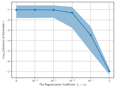
Figure 1: The Logarithm of the variations in the solutions for $\bm{\pi}$. The variation is measured as the sum of the eigenvalues of the covariance matrix of the solutions (i.e., nuclear norm). The shaded area shows the [5, 95] percentile.

Appendix C Algorithms

Algorithm 1 Shapley Context Method (SCM)

0:  An instruction-tuned LLM $M$ that generates outputs $y$ for each query $q$ and context $c$.

0:  A set of queries $Q=\{q_{1},\ldots,q_{m}\}$.

0:  A set of datasets that we need to compute their contributions $D_{1},\ldots,D_{K}$.

1:  for $q\in Q$ do

2:     Compute output without context: $y=M(q)$.

3:     for $S\subset\{D_{1},\ldots,D_{K}\}\setminus\{D_{k}\}$ do

4:        Use RAG to create contexts $c_{S}$ and $c_{S\cup\{D_{k}\}}$ from the datasets in $S$ and $D_{k}$.

5:        Compute the output with the context $y|c_{S}=M(q|c_{S})$.

6:        Compute the output with the context including $D_{k}$: $y|c_{S\cup\{D_{k}\}}=M(q|c_{S\cup\{D_{k}\}})$.

7:        Compute the similarities $s_{S}$ and $s_{S\cup\{k\}}$ using Eq. (2).

8:        Compute the residual gain $r_{k,S}=s_{S\cup\{k\}}-s_{S}$.

9:     end for

10:     Use Eq. (3) and $r_{k,S}$ to compute $\phi_{k}(q)$.

11:  end for

12:  Return average $\phi_{k}$ over $m$ queries.

Algorithm 2 Context Mixture Factorization (CMF)

0:  An instruction-tuned LLM $M$ that generates outputs $y$ for each query $q$ and context $c$.

0:  A set of queries $Q=\{q_{1},\ldots,q_{m}\}$.

0:  A set of datasets that we need to compute their contributions $D_{1},\ldots,D_{K}$.

1:  for $q\in Q$ do

2:     Compute output without context: $p[y|q,c_{0}]=M(q)$.

3:     for $k=1,\ldots,K$ do

4:        Use RAG to create context $c_{k}$ from the dataset $D_{k}$.

5:        Compute the output with the context $p[y|q,c_{k}]=M(q|c_{k})$.

6:     end for

7:  end for

8:  Build matrix $P$, where $P_{k,j}=p[y|q_{j},c_{k}]$.

9:  Solve Eq. (7) via alternating least squares and to compute $\widehat{\bm{\pi}}$.

10:  Return the contribution vector $\widehat{\bm{\pi}}$.

Appendix D Implementation Details

D.1 Prompt Engineering

For simplicity of evaluation and without loss of generality, we used BoolQ (Clark et al., 2019) Q&A dataset, where the answers are binary Yes/No. To instruct the LLMs to provide direct boolean responses, we used prompt engineering. Initially, we tested various prompts without explicitly instructing the model to answer with ”Yes” or ”No.” Diverse examples used in this process are provided in Appendix D.3. Through iterative testing, we found that responses improved when the model was explicitly instructed to provide a boolean answer. This led to our final prompt:

Prompt: ”Given the context below, answer the question that follows with only ’Yes’, ’No’, or ’I don’t know’ if the context is insufficient.
{question}? The answer to this question is”

While this final prompt worked well for GPT-4, Bloomz, and Mistral 7B, generating straightforward ”Yes,” ”No,” or ”I don’t know” responses, it was harder to instruct Phi-3-mini. Even with the final prompt, Phi-3-mini often generated more text than just a simple boolean response.

Therefore, calculating similarities was straightforward for GPT-4, Bloomz, and Mistral 7B, but we had to devise another solution for Phi-3-mini. The embedding similarity API on GPT-4 was not precise enough as it did not focus primarily on the context of the generated response. To calculate the similarity for Phi-3-mini, we created a Zero-shot classification layer (which takes 1000 characters) between the prediction and the result to measure similarity more accurately.

D.2 Using RAG

Given the limitations of LLM context windows, fitting entire datasets directly into the context is impractical. To address this, we utilized Retrieval-Augmented Generation (RAG) (Lewis et al., 2020) to enhance the context by retrieving relevant documents from databases before generating responses. The process involves splitting the documents into semantically relevant chunks using the RecursiveCharacterTextSplitter from the Hugging Face Transformers library, computing embeddings for all chunks with a model like thenlper/gte-small, and storing these embeddings in a vector database using FAISS (Facebook AI Similarity Search). When a question is posed, it is embedded and a similarity search is performed against the vector database to find the closest matching documents. These retrieved documents are then provided as context to the LLMs along with the original question, allowing the LLMs to generate responses augmented with additional context.

We used a chunk size of 512 and a top-k value of 3, ensuring the context was trimmed to 2000 characters for conciseness.

D.3 Prompts

General Question Prompt: “Read the context provided and answer the following question: {question}”

Contextual Understanding Prompt: “Based on the information in the context, what can you conclude about the following question? {question}”

Summarization Prompt: “After considering the context below, summarize your answer to this question: {question}”

Opinion-Based Prompt: “Given the details in the context, what is your opinion on the following question: {question}”

Detail Extraction Prompt: “Extract relevant information from the context to answer this question: {question}”

Fact-Checking Prompt: “Using the context provided, verify the accuracy of the following statement: {question}”

Table 5 shows the average accuracy calculated by comparing the predictions with the ground truth from BoolQ.

References

- Abdin et al. (2024) Marah Abdin, Sam Ade Jacobs, Ammar Ahmad Awan, Jyoti Aneja, Ahmed Awadallah, Hany Awadalla, Nguyen Bach, Amit Bahree, Arash Bakhtiari, Harkirat Behl, et al. Phi-3 technical report: A highly capable language model locally on your phone. arXiv preprint arXiv:2404.14219, 2024.
- Achiam et al. (2023) Josh Achiam, Steven Adler, Sandhini Agarwal, Lama Ahmad, Ilge Akkaya, Florencia Leoni Aleman, Diogo Almeida, Janko Altenschmidt, Sam Altman, Shyamal Anadkat, et al. GPT-4 Technical Report. arXiv:2303.08774, 2023.
- Chen et al. (2021) Yuanyuan Chen, Boyang Li, Han Yu, Pengcheng Wu, and Chunyan Miao. Hydra: Hypergradient data relevance analysis for interpreting deep neural networks. In AAAI, volume 35, pp. 7081–7089, 2021.
- Clark et al. (2019) Christopher Clark, Kenton Lee, Ming-Wei Chang, Tom Kwiatkowski, Michael Collins, and Kristina Toutanova. Boolq: Exploring the surprising difficulty of natural yes/no questions. In NAACL-HLT, 2019.
- Feldman & Zhang (2020) Vitaly Feldman and Chiyuan Zhang. What neural networks memorize and why: Discovering the long tail via influence estimation. NeurIPS, 33:2881–2891, 2020.
- Ghorbani & Zou (2019) Amirata Ghorbani and James Zou. Data shapley: Equitable valuation of data for machine learning. In International conference on machine learning, pp. 2242–2251. PMLR, 2019.
- Ginart et al. (2019) Antonio Ginart, Melody Guan, Gregory Valiant, and James Y Zou. Making ai forget you: Data deletion in machine learning. NeurIPS, 32, 2019.
- Gorski et al. (2007) Jochen Gorski, Frank Pfeuffer, and Kathrin Klamroth. Biconvex sets and optimization with biconvex functions: a survey and extensions. Mathematical methods of operations research, 66(3):373–407, 2007.
- Hammoudeh & Lowd (2024) Zayd Hammoudeh and Daniel Lowd. Training data influence analysis and estimation: A survey. Machine Learning, pp. 1–53, 2024.
- Jiang et al. (2023) Albert Q Jiang, Alexandre Sablayrolles, Arthur Mensch, Chris Bamford, Devendra Singh Chaplot, Diego de las Casas, Florian Bressand, Gianna Lengyel, Guillaume Lample, Lucile Saulnier, et al. Mistral 7b. arXiv preprint arXiv:2310.06825, 2023.
- Koh & Liang (2017) Pang Wei Koh and Percy Liang. Understanding black-box predictions via influence functions. In International conference on machine learning, pp. 1885–1894. PMLR, 2017.
- Le Scao et al. (2023) Teven Le Scao, Angela Fan, Christopher Akiki, Ellie Pavlick, Suzana Ilić, Daniel Hesslow, Roman Castagné, Alexandra Sasha Luccioni, François Yvon, Matthias Gallé, et al. Bloom: A 176b-parameter open-access multilingual language model. 2023.
- Lewis et al. (2020) Patrick Lewis, Ethan Perez, Aleksandra Piktus, Fabio Petroni, Vladimir Karpukhin, Naman Goyal, Heinrich Küttler, Mike Lewis, Wen-tau Yih, Tim Rocktäschel, et al. Retrieval-augmented generation for knowledge-intensive nlp tasks. NeurIPS, 2020.
- Nguyen et al. (2023) Elisa Nguyen, Minjoon Seo, and Seong Joon Oh. A bayesian perspective on training data attribution. arXiv preprint arXiv:2305.19765, 2023.
- Nohyun et al. (2022) Ki Nohyun, Hoyong Choi, and Hye Won Chung. Data valuation without training of a model. In The Eleventh International Conference on Learning Representations, 2022.
- Park et al. (2023) Sung Min Park, Kristian Georgiev, Andrew Ilyas, Guillaume Leclerc, and Aleksander Madry. Trak: attributing model behavior at scale. In ICML, 2023.
- Pruthi et al. (2020) Garima Pruthi, Frederick Liu, Satyen Kale, and Mukund Sundararajan. Estimating training data influence by tracing gradient descent. NeurIPS, 33:19920–19930, 2020.
- Sekhari et al. (2021) Ayush Sekhari, Jayadev Acharya, Gautam Kamath, and Ananda Theertha Suresh. Remember what you want to forget: Algorithms for machine unlearning. NeurIPS, 34:18075–18086, 2021.
- Shapley (1953) L S Shapley. A value for n-person games. Contributions to the Theory of Games, pp. 307–317, 1953.
- Worledge et al. (2024) Theodora Worledge, Judy Hanwen Shen, Nicole Meister, Caleb Winston, and Carlos Guestrin. Unifying corroborative and contributive attributions in large language models. In 2024 IEEE Conference on Secure and Trustworthy Machine Learning (SaTML), pp. 665–683. IEEE, 2024.