Density Matrices for Metaphor Understanding

Abstract

In physics, density matrices are used to represent mixed states, i.e. probabilistic mixtures of pure states. This concept was used to model lexical ambiguity in [32]. In this paper, we consider metaphor as a type of lexical ambiguity, and examine whether metaphorical meaning can be effectively modelled using mixtures of word senses. We find that modelling metaphor is significantly more difficult than other kinds of lexical ambiguity, but that our best-performing density matrix method outperforms simple baselines as well as some neural language models.

1 Introduction

The use of vectors to model word meaning forms the basis of all modern approaches to modelling language. The idea behind this approach is called distributional semantics – using the distributions of words in text to build vectors that encode word meanings. When we have built vectors for words, say we have $\ket{\textit{cat}}$, $\ket{\textit{kitten}}$, and $\ket{\textit{orthodontist}}$, the hope is that words that have similar meanings will be close together in the vector space, and that words that have dissimilar meanings are further apart, where we measure distance between words as the inner product of the normalised vectors, or equivalently as the cosine similarity, i.e., the cosine of the angle between the vectors. So, for example, we should have that:

$$\braket{cat}{kitten}>\braket{cat}{orthodontist}$$

However, representing words as vectors has some clear disadvantages. Firstly, words can have more than one meaning, and a naïve approach to building word vectors will try to pack all those meanings into one vector—ending up with a representation somewhere in the middle. Secondly, as well as representing word meanings we also wish to represent phrases, sentences, and paragraphs of text. However, simply representing words as vectors does not give us an obvious way of composing word vectors to produce phrase or sentence vectors.

There have been a number of approaches to representing ambiguity for word vectors. The task of discriminating different senses of a given word (word sense discrimination or WSD), is often framed as a classification task: given a sentence with a particular word, identify the sense of that word from its context [21, 37, 30]. An alternative task is to identify the sense of every word in a sentence. WSD can become a complex task, since each word must be disambiguated with respect to each other word in the sentence. One approach is simply to disambiguate word meanings in advance, and learn different vectors for different senses of a word. However, given that any word may have multiple meanings, this approach could generate a large number of possible meaning combinations that need to be disambiguated. Instead, we would like to be able to compose words together, and for a sentence to be disambiguated in the process of composition.

A key manifestation of ambiguity in language is the use of metaphor. Metaphor is pervasive in speech, with some estimates showing that we use metaphors on average every 3 sentences. As such, language models need to be able to deal with metaphor when it occurs. Many metaphorical uses are what is known as ‘conventional’ metaphor. This means that the metaphor has become entrenched in language, and can therefore be seen as a case of lexical ambiguity. For example, the most basic use of the word bright is as applied to colour. However, we often use this word to mean ‘intelligent’, as in bright student. This meaning of the word was created metaphorically from the original meaning of ‘colourful’, but has now become conventionalised in language.

The field of compositional distributional semantics [4, 11, 28] looks at systematic ways to compose word vectors together that are guided by our knowledge of grammatical composition. This paper works within the framework proposed by [11], which has fundamental links to quantum theory. Within [11], the structure of a sentence, together with the meanings of the words in the sentence, can be viewed as a tensor network creating the meaning of the sentence as a whole. This is further developed and indeed implemented on quantum computers in [24].

In the current work, we look at the ability of density matrices to represent the ambiguity represented by conventional metaphor. [32] show how density matrices and completely positive maps can be integrated with the compositional distributional semantics proposed by [11], and these methods are extended in [25]. The methods developed by [32] and applied in [25] are very successful, beating state of the art language models. We investigate whether density matrix methods are as effective in modelling conventional metaphor as they are in standard cases of lexical ambiguity.

In this paper, we firstly (section 2) give an overview of how density matrices have been used in NLP to model lexical entailment and semantics and syntactic ambiguity. In section 3 we review the quantum-inspired approach to NLP originally proposed by [11] which extends distributional semantics models to include composition, including how density matrices can be used in this compositional framework, and in section 4 how density matrices can be built automatically from text. We introduce a new dataset to test how well our implementations are able to model metaphor (Section 5), and finally, report results on this new dataset (Section 6), finding that metaphor interpretation is a difficult task for all models tested, although some density matrix methods perform above baseline.

2 Related Work: Density Matrices in Natural Language Processing

Two key uses of density matrices in NLP are 1) to model hyponymy and ambiguity, and 2) to model lexical ambiguity. We summarize research in these areas.

Density Matrices for Lexical Entailment

Vectors are not well suited for representing hyponymy (is-a) relations between words. However, since density matrices can be ordered using a variant of the Löwner ordering [41], they are a candidate for representing these relations. This was investigated in [36], where density matrices were used to model hyponymy between words and phrases. This work models the strength of a hyponymy relation between two words as a function of the KL-divergence between the two matrices of the words. This measure has the nice property that hyponymy relationships between individual words lift to an entailment relationship between the two sentences. For example, given that clarify is a hyponym of explain and rule is a hyponym of process, we would expect that the phrase clarify rule entails explain process. In similar work, [3] model the relationship of hyponymy as the Löwner order between two matrices. The Löwner order states that $A\leqslant B$ iff $0\leqslant B-A$. [3] provide a measure of graded hyponymy between two matrices which again lifts to entailment at the sentence level. [22] proposes a method for building density matrices using information from WordNet together with off-the shelf word vectors such as word2vec or GloVe. Density matrices for words can be composed to form density matrices for phrases and sentences by a variety of operators such as addition, pointwise multiplication, or more complex operators, such as BMult/Phaser [9, 22, 32] and KMult/Fuzz [9, 22]. These representations and composition operators work well on a simple entailment task from [18].

The use of density matrices to model logical and conversational entailment is developed further in [23, 35, 39], who develop a notion of negation for density matrices. [35, 39] extend these ideas to include the notion of conversational negation [19]. This can be thought of as modelling the acceptability of a sentence such as ‘That’s not a dog, it’s a wolf’ vs ‘That’s not a dog, it’s a rainbow’. If we view negation as purely logical, then these sentences should be viewed as equally acceptable. In contrast, conversational negation provides a set of alternatives. [35, 39] model this by narrowing the subspace spanned by the logical negation to give a set of relevant alternatives. They furthermore provide alternative models of negation that utilize the Moore-Penrose pseudo-inverse of a matrix. In [14], the monotonicity of composition operators with respect to the Löwner order is investigated.

Another approach to building density matrices for entailment was developed by [6]. In this work, the authors model language as a set of sequences $S$ from a given vocabulary, together with a probability distribution over this set. They form the free vector space over the set of sequences $S$, and then form a rank-1 density operator which encodes the probability distribution over sequences that models the language. Reduced density operators may be formed by tracing out over particular subspaces, and they show that in doing so, the hierarchy of subsequences is encoded by the Löwner order over these density matrices. This means that they can, for example, encode the fact that black cats are a subclass of cats - something that is not done by the approach outlined in [36] or [3].

Density Matrices for Ambiguity

Using density matrices to model ambiguity in natural language is very natural. Density matrices were introduced in quantum physics to encode the notion of a mixed state: the case where the state of a system is not known. In this case, the system is encoded by taking a mixture of the possible states that it could be in. In the case of language, if we consider a word on its own, it may have multiple senses, and without context we cannot tell what the meaning of the word is. For example, table on its own can mean a piece of furniture, a structure for storing data, the act of presenting a topic, and so on. If we can store multiple different senses of a word in one representation, this can help to represent language.

One of the first uses of density matrices to represent ambiguity in text was [5]. This work aims to build representations of words that can encode multiple different kinds of word usage within one representation. For example, consider the word table. This word is semantically ambiguous: table means something different in ‘Your dinner is on the table’ vs. ‘The data is in the table’. It is also syntactically ambiguous, since we can use it as a verb: ‘table a motion’. The standard way of building word vectors forms a superposition of all these senses. [5] firstly build a space that takes into account the grammatical role of words, as encoded by dependency relations. They then form density matrices for individual words, based on the grammatical relations that word can participate in. The representations they learn are effective at the word level, but they do not give any methods for composing words together. [13] also use density matrix representations to model syntactic ambiguity. They show to to model alternative syntactic structures within one whole, and show how word representations can be composed.

[32] provide a thorough and elegant theoretical grounding that describes how to use the categorical compositional methods of [11] with density matrix representations of words. This will be described fully in subsequent sections. The main idea behind this is that words are represented as probabilistic mixtures of their senses, and that when words are composed to make phrases, the phrase should disambiguate the meaning of the ambiguous word. The amount of ambiguity in a word can be represented as von Neumann entropy. [32] carry out corpus-based experiments, and show that the von Neumann entropy of word representations reduces in composition, indicating that the words have been disambiguated.

[25] extend the work of [32] to provide a means of building density matrices automatically from large scale text corpora. We describe this method in detail later in the paper. [25] test their density matrix representations on a range of datasets designed to test the ability of compositional models to disambiguate word meanings. Their representations outperform compositional baselines as well as state of the art large neural models.

3 Categorical Compositional Distributional Semantics

We work in the framework of categorical compositional distributional semantics [11]. In brief, words are represented as vectors inhabiting vector spaces that match their grammatical type. Setting a vector space $N$ to be the noun type, and another space $S$ to be the sentence type, we model nouns as vectors, adjectives as linear maps $adj:N\rightarrow N$ and verbs as multilinear maps from copies of $N$ to $S$.

3.1 Pregroup Grammars

In order to describe grammatical structure we use Lambek’s pregroup grammars [20]. A pregroup $(P,\leq,\cdot,1,(-)^{l},(-)^{r})$ is a partially ordered monoid $(P,\leq,\cdot,1)$ where each element $p\in P$ has a left adjoint $p^{l}$ and a right adjoint $p^{r}$, such that the following inequalities hold:

$$p^{l}\cdot p\leq 1\leq p\cdot p^{l}\quad\text{ and }\quad p\cdot p^{r}\leq 1\leq p^{r}\cdot p$$ (1)

We think of the elements of a pregroup as linguistic types. Concretely, we will use an alphabet $\mathcal{B}=\{n,s\}$. We use the type $s$ to denote a declarative sentence and $n$ to denote a noun. A transitive verb can then be denoted $n^{r}sn^{l}$. If a string of words and their types reduces to the type $s$, the sentence is judged grammatical. The sentence Junpa loves cats is typed $n~{}(n^{r}sn^{l})~{}n$, and can be reduced to $s$ as follows:

$$n~{}(n^{r}sn^{l})~{}n\leq 1\cdot sn^{l}n\leq 1\cdot s\cdot 1\leq s$$

3.2 Compositional Distributional Models

We interpret a pregroup grammar as a compact closed category, a structure shared by the category of finite dimensional Hilbert spaces. We briefly describe here the structure of a compact closed category, but for more details, please see [11, 33] and the introduction to relevant category theory given in [10].

Distributional vector space models live in the category $\mathbf{FHilb}$ of finite dimensional real Hilbert spaces and linear maps. $\mathbf{FHilb}$ is compact closed. Each object $V$ is its own dual and the left and right unit and counit morphisms coincide. Given a fixed basis $\{\ket{v_{i}}\}_{i}$ of $V$, the unit $\eta$ and counit $\epsilon$ are defined as:

$$\eta:\mathbb{R}\rightarrow V\otimes V::1\mapsto\sum_{i}\ket{v_{i}}\otimes\ket{v_{i}}\qquad\epsilon:V\otimes V\rightarrow\mathbb{R}::\sum_{ij}c_{ij}\ket{v_{i}}\otimes\ket{v_{j}}\mapsto\sum_{i}c_{ii}$$

3.3 Grammatical Reductions in Vector Spaces

Following [33], reductions of the pregroup grammar are mapped into the category $\mathbf{FHilb}$ of finite dimensional Hilbert spaces and linear maps using a strong monoidal functor $\mathsf{Q}$ which preserves the compact closed structure:

$$\mathsf{Q}:\mathbf{Preg}\rightarrow\mathbf{FHilb}$$

We map noun and sentence types to appropriate finite dimensional vector spaces $\mathsf{Q}(n)=N$ $\mathsf{Q}(s)=S$, and concatenation in $\mathbf{Preg}$ is mapped to the tensor product in $\mathbf{FHilb}$. Each type reduction $\alpha$ in the pregroup is mapped to a linear map in $\mathbf{FHilb}$. Given a grammatical reduction $\alpha:p_{1},p_{2},...p_{n}\rightarrow s$ and word vectors $\ket{w_{i}}$ with types $p_{i}$, a vector representation of the sentence $w_{1}w_{2}...w_{n}$ is given by:

$$\ket{w_{1}w_{2}...w_{n}}=\mathsf{Q}(\alpha)(\ket{w_{1}}\otimes\ket{w_{2}}\otimes...\otimes\ket{w_{n}})$$

We use the inner product to compare meanings of sentences by computing the cosine distance between sentence vectors. So, if sentence $s$ has vector representation $\ket{s}$ and sentence $s^{\prime}$ has representation $\ket{s^{\prime}}$, their degree of synonymy is given by:

$$\frac{\braket{s}{s^{\prime}}}{\sqrt{\braket{s}{s}\braket{s^{\prime}}{s^{\prime}}}}$$

3.4 Density Matrices in Categorical Compositional Distributional Semantics

Categorical compositional distributional semantics was extended in [32] to model nouns as density matrices in $N\otimes N$ and adjective and verbs as completely positive maps.

In distributional models of meaning, density matrices have been used in a variety of ways. We consider the meaning of a word $w$ to be given by a collection of unit vectors $\{\ket{w_{i}}\}_{i}$. Each $\ket{w_{i}}$ is weighted by $p_{i}\in[0,1]$, such that $\sum_{i}p_{i}=1$. Then the density operator:

$$\llbracket w\rrbracket=\sum_{i}p_{i}\ket{w_{i}}\bra{w_{i}}$$

represents the word $w$. In [32], the vectors $\{\ket{w_{i}}\}_{i}$ are interpreted as senses of a given word, and we will use this interpretation later in the paper. In [3, 2, 22], the vectors $\{\ket{w_{i}}\}_{i}$ are interpreted as exemplars of a concept, and in [5] the $\{\ket{w_{i}}\}_{i}$ are interpreted as instances of use of a word.

3.5 The CPM Construction

Applying Selinger’s CPM construction [38] to $\mathbf{FHilb}$ produces a new compact closed category in which the states are positive operators. This construction has previously been used in a linguistic setting in [17, 32, 2, 3, 22]. Throughout this section $\mathcal{C}$ denotes an arbitrary ${\dagger}$-compact closed category.

Definition 1 (Completely positive morphism [38])

A $\mathcal{C}$-morphism $\varphi:A^{*}\otimes A\rightarrow B^{*}\otimes B$ is said to be completely positive if there exists $C\in\mathsf{Ob}(\mathcal{C})$ and $k\in\mathcal{C}(C\otimes A,B)$, such that $\varphi$ can be written in the form:

$$(k_{*}\otimes k)\circ(1_{A^{*}}\otimes\eta_{C}\otimes 1_{A})$$

Identity morphisms are completely positive, and completely positive morphisms are closed under composition in $\mathcal{C}$, leading to the following:

Definition 2 ($\mathbf{CPM}(\mathcal{C})$ [38])

If $\mathcal{C}$ is a ${\dagger}$-compact closed category then $\mathbf{CPM}(\mathcal{C})$ is a category with the same objects as $\mathcal{C}$ and its morphisms are the completely positive morphisms.

The $\dagger$-compact structure required for interpreting language in our setting lifts to $\mathbf{CPM}(\mathcal{C})$:

Theorem 1 (Compact Closure [38])

$\mathbf{CPM}(\mathcal{C})$ is also a $\dagger$-compact closed category. There is a functor:

$$\mathsf{E}:\mathcal{C} \rightarrow\mathbf{CPM}(\mathcal{C})$$

$$k \mapsto k_{*}\otimes k$$

This functor preserves the $\dagger$-compact closed structure, and is faithful “up to a global phase”.

3.5.1 Sentence Meaning in the category $\mathbf{CPM}(\mathbf{FHilb})$

In the vector space model of distributional models of meaning the movement from syntax to semantics was achieved via a strong monoidal functor $\mathsf{Q}:\mathbf{Preg}\rightarrow\mathbf{FHilb}$. Language can be assigned semantics in $\mathbf{CPM}(\mathbf{FHilb})$ in an entirely analogous way via a strong monoidal functor:

$$\mathsf{S}:\mathbf{Preg}\rightarrow\mathbf{CPM}(\mathbf{FHilb})$$

If $w_{1},w_{2}...w_{n}$ is a string of words with corresponding grammatical types $t_{i}$ in $\mathbf{Preg}_{\mathcal{B}}$. and the type reduction is given by $t_{1},...t_{n}\xrightarrow{r}x$ for some $x\in\mathsf{Ob}(\mathbf{Preg}_{\mathcal{B}}$, where $\llbracket w_{i}\rrbracket$ is the meaning of word $w_{i}$ in $\mathbf{CPM}(\mathbf{FHilb})$, i.e. a density matrix $\rho_{i}$. Then the meaning of $w_{1}w_{2}...w_{n}$ is given by:

$$\llbracket w_{1}w_{2}...w_{n}\rrbracket=\mathsf{S}(r)(\llbracket w_{1}\rrbracket\otimes...\otimes\llbracket w_{n}\rrbracket)$$

We render semantic similarity of representations as the generalised inner product, i.e. $\mathrm{Tr}(\llbracket w_{1}\rrbracket^{\dagger}\llbracket w_{2}\rrbracket)$, as do [32]. This notion of semantic similarity is modulated by the extent of the ambiguity of a representation. If a representation is maximally ambiguous, that is, $\llbracket w_{1}\rrbracket=\mathbb{I}/n$, then the similarity of $\llbracket w_{1}\rrbracket$ with itself is only $1/n$. We choose to interpret this as reflecting the fact that the meaning of of $\textit{w}_{1}$ is undetermined without further context, and hence that the two instances of $\textit{w}_{1}$ being compared could in fact have different senses. On the other hand, if $\llbracket w_{1}\rrbracket$ is pure, then self-similarity is 1, as expected.

We now go on to describe how density matrices can be learnt directly from text corpora, and composed to form sentence representations. We will assess these representations in a setting requiring metaphor interpretation.

We now have all the ingredients to derive sentence meanings in $\mathbf{CPM}(\mathbf{FHilb})$.

Example 1

We firstly show that the results from $\mathbf{FHilb}$ lift to $\mathbf{CPM}(\mathbf{FHilb})$. Let the noun space $N$ be a real Hilbert space with basis vectors given by $\{\ket{n_{i}}\}_{i}$, where for some $i$, $\ket{n_{i}}=\ket{\textit{shoulders}}$ Let the sentence space be another space $S$ with basis $\{\ket{s_{i}}\}_{i}$. The verb $\ket{\textit{slouch}}$ is given by:

$$\ket{\textit{slouch}}=\sum_{pq}C_{pq}\ket{n_{p}}\otimes\ket{s_{q}}$$

The density matrix for the noun shoulders is in fact a pure state given by:

$$\llbracket\textit{shoulders}\rrbracket=\ket{n_{i}}\bra{n_{i}}$$

and similarly, $\llbracket\textit{slouch}\rrbracket$ in $\mathbf{CPM}(\mathbf{FHilb})$ is:

$$\llbracket\textit{slouch}\rrbracket=\sum_{pqtu}C_{pq}C_{tu}\ket{n_{p}}\bra{n_{t}}\otimes\ket{s_{q}}\bra{s_{u}}$$

The meaning of the composite sentence is simply $(\varepsilon_{N}\otimes 1_{S})$ applied to $(\llbracket\textit{shoulders}\rrbracket\otimes\llbracket\textit{slouch}\rrbracket)$. This corresponds to:

$$\llbracket\textit{shoulders slouch}\rrbracket =\varphi(\llbracket\textit{shoulders}\rrbracket\otimes\llbracket\textit{slouch}\rrbracket)$$

$$=\sum_{qu}C_{iq}C_{iu}\ket{s_{q}}\bra{s_{u}}$$

This is a pure state corresponding to the vector $\sum_{q}C_{iq}\ket{s_{q}}$.

We can also deal with mixed states.

Example 2

Let the noun space $N$ be a real Hilbert space with basis vectors given by $\{\ket{n_{i}}\}_{i}$. Consider two senses of the word shoulder meaning 1) a part of your body and 2) the edge of a road. Let:

$$\ket{\textit{shoulder}_{\textit{body}}}=\sum_{i}a_{i}\ket{n_{i}},\>\ket{\textit{shoulder}_{\textit{road}}}=\sum_{i}b_{i}\ket{n_{i}}$$

and with the sentence space $S$, consider the word slump with the senses slouch and decline we define:

$$\ket{\textit{slump}_{\textit{slouch}}} =\sum_{pqr}C_{pqr}\ket{n_{p}}\otimes\ket{s_{q}}$$

$$\ket{\textit{slump}_{\textit{decline}}} =\sum_{pqr}D_{pqr}\ket{n_{p}}\otimes\ket{s_{q}}$$

We set:

$$\llbracket\textit{shoulder}\rrbracket =\frac{1}{2}(\ket{\textit{shoulder}_{\textit{body}}}\bra{\textit{shoulder}_{\textit{body}}}+\ket{\textit{shoulder}_{\textit{road}}}\bra{\textit{shoulder}_{\textit{road}}})$$

$$\llbracket\textit{slump}\rrbracket =\frac{1}{2}(\ket{\textit{slump}_{\textit{slouch}}}\bra{\textit{slump}_{\textit{slouch}}}+\ket{\textit{slump}_{\textit{decline}}}\bra{\textit{slump}_{\textit{decline}}})$$

Then, the meaning of the sentence:

$$s=\textit{Shoulders slump}$$

is given by:

$$\llbracket s\rrbracket=(\varepsilon_{N}\otimes 1_{S}\otimes\varepsilon_{N})(\llbracket\textit{shoulders}\rrbracket\otimes\llbracket\textit{slump}\rrbracket$$

In the example above, we have a two word sentence where each word has two interpretations. There are therefore 4 possible assignments of senses to the words. However, only one assignment of words makes sense in context. The aim is for the correct senses of each word to be picked out in composition.

4 Methods

4.1 Learning Density Matrices from Text

[25] introduce a method for learning density matrices from text called Multi-sense Word2DM. This is an extension of the word2vec skipgram with negative sampling (SGNS) [26] to density matrices. word2vec learns vectors for words by running through a large corpus of text and updating word vectors according to the following objective function with regard to model parameters $\theta$:

$$J(\theta)=\log\sigma(\braket{v_{t}}{v_{c}})+\sum_{k=1}^{K}\log\sigma(-\braket{v_{t}}{v_{k}})$$ (2)

where $v_{t}$ is the embedding of target word, $v_{c}$ is the embedding of the context word, $v_{1},v_{2},...,v_{K}$ are the embeddings of $K$ negative samples, and $\sigma$ is the logistic function. Maximising equation 2 adjusts the embeddings of words occurring in the same context to be more similar and adjusts the embeddings of words that don’t occur together to be less similar. Multi-sense Word2DM is a modification of SGNS for density matrices. Instead of learning one vector per word, multiple sense embeddings are learnt and then combined together to form a density matrix. Each sense of a word has its own $n$-dimensional embedding. A density matrix can be expressed in terms of the sense embeddings as

$$A=BB^{\dagger}=\sum_{i=1}^{m}\ket{b_{i}}\bra{b_{i}}$$ (3)

where $\ket{b_{1}},...,\ket{b_{m}}$ are the columns of $B$ corresponding to different senses. Each word is also associated with a single vector $v_{w}$, which represents it as a context word. The following objective function is maximised:

$$J(\theta)=\log\sigma(\braket{b_{t}}{c_{t}})+\sum_{k=1}^{K}\log\sigma(-\braket{b_{t}}{v_{w_{k}}})$$ (4)

where $\ket{c_{t}}$ is the sum of context vectors for all words surrounding the target word and $\ket{b_{t}}$ is the the embedding for the relevant sense of the target word. We select $\ket{b_{t}}$ by finding the column of $B_{t}$ most similar to $\ket{c_{t}}$ (measured by cosine similarity). Multi-sense Word2DM explicitly models ambiguity by letting the columns of the intermediary matrix represent the different senses of a word. During training the column closest to the context embedding is selected as the relevant sense embedding and only this column is updated.

4.2 Composition Methods

The methods used by [25] to build density matrices only build matrices that inhabit a single space $W\otimes W$, rather than the larger spaces needed for verbs and adjectives. Because of this, [25] use a set of composition methods that can be seen as ‘lifting’ a given word representation to the type needed for composition. These are based on methods in [22, 9], and we will use these in section 6. We view relational words such as adjectives or verbs as maps that takes nouns as arguments. The composition methods are as follows, using the example of an adjective modifying a noun:

• Add: $\llbracket adj\rrbracket+\llbracket noun\rrbracket$

• Mult: $\llbracket adj\rrbracket\odot\llbracket noun\rrbracket$

• Fuzz: $\sum_{i}p_{i}\,P_{i}\,\llbracket noun\rrbracket\,P_{i}$, where $\sum_{i}p_{i}\,P_{i}\,$ is the spectral decomposition of $\llbracket adj\rrbracket$

• Phaser: $\llbracket adj\rrbracket^{1/2}\llbracket noun\rrbracket\llbracket adj\rrbracket^{1/2}$

More complex phrases are combined according to their parse. So, a transitive sentence modified with an adjective is composed as $(\text{subj}(\text{verb}(\text{adj obj})))$. Composing e.g. the sentence Junpa likes stripy cats would consist of the following steps:

$$\llbracket\textit{stripy cats}\rrbracket =f(\llbracket\textit{stripy}\rrbracket,\llbracket\textit{cats}\rrbracket)$$ (5)

$$\llbracket\textit{likes stripy cats}\rrbracket =f(\llbracket\textit{likes}\rrbracket,\llbracket\textit{stripy cats}\rrbracket)$$ (6)

$$\llbracket\textit{Junpa likes stripy cats}\rrbracket =f(\llbracket\textit{Junpa}\rrbracket,\llbracket\textit{likes stripy cats}\rrbracket)$$ (7)

where the composer $f$ can be substituted by any of the composition methods listed above.

5 Implementation

5.1 Datasets and Tasks

We build a novel dataset to test disambiguation in a metaphorical context. The basic structure of the dataset is as follows. Given a target sentence that uses a metaphorical word, we minimally alter the target sentence to provide an apt literal paraphrase and an inapt paraphrase of the sentence. We attempt to replace only the single metaphorically used word, although this is not always possible.

Example

• Target sentence: He showered her with presents

• Apt paraphrase: He gave her presents

• Inapt paraphrase: He sprinkled her with presents

The expectation is that the apt paraphrase is semantically closer to the target sentence than the inapt sentence is. So, given representations $\llbracket target\rrbracket$, $\llbracket apt\rrbracket$, $\llbracket inapt\rrbracket$, $\mathrm{Tr}(\llbracket target\rrbracket^{\dagger}\llbracket apt\rrbracket)>\mathrm{Tr}(\llbracket target\rrbracket^{\dagger}\llbracket inapt\rrbracket)$.

We use the metaphorical sentences and their literal paraphrases from [29], and generate inapt paraphrases as follows. Each target sentence includes one metaphorically used verb. We use WordNet [27] to determine the most commonly used sense of the verb. WordNet is a resource listing words, their different senses (called ‘synsets’), synonyms within each synset, and hyponym, hypernym and other relations between words. The synsets are listed in order of frequency, so that the first synset is the most commonly used sense of a word. We expect that the most commonly used sense of a word will be a literal sense, and that taking a synonym from this sense will form an inapt paraphrase, as in the example above. We manually inspect each candidate inapt paraphrase, and if the paraphrase is not inapt, we generate a new paraphrase by looking at synonyms of the hypernym of the metaphorically used word. We generated inapt paraphrases for a total of 171 metaphorical sentences.

We then simplified the sentences to consist of just subject-verb (SV), verb-object (VO) or subject-verb-object (SVO) fragments, and subsequently padded these fragments with pronouns and determiners to generate simplified versions of the full sentences. This usually just involved a shortening of the sentence. We test our models on two versions of the dataset. The dataset in the format of SV/VO/SVO fragments we call the short-form dataset, and the dataset with full but simplifed sentences we call the long-form dataset.

Simplification Procedure

• Original sentence: He wasted his inheritance on his insincere friends.

• VO format: waste inheritance

• Simplified sentence: She wasted her inheritance

Human Annotation

We solicited annotations from humans as follows. We gave them triples of target sentence, apt paraphrase, and inapt paraphrase. The apt and inapt paraphrases were presented in a random order: sometimes the apt was presented first, and sometimes the inapt. Participants were asked to state which was the best paraphrase of the target sentence, and then to rate the similarity of each paraphrase to the target sentence. All participants were asked to annotate all 171 triples, resulting in 10 annotations per triple. Triples were presented in a random order for each participant. Mean inter-annotator agreement, calculated using Spearman’s rho over all pairs of annotators, was 0.589, which is a reasonable level. Examples of the annotation task are shown in figures 1 and 2

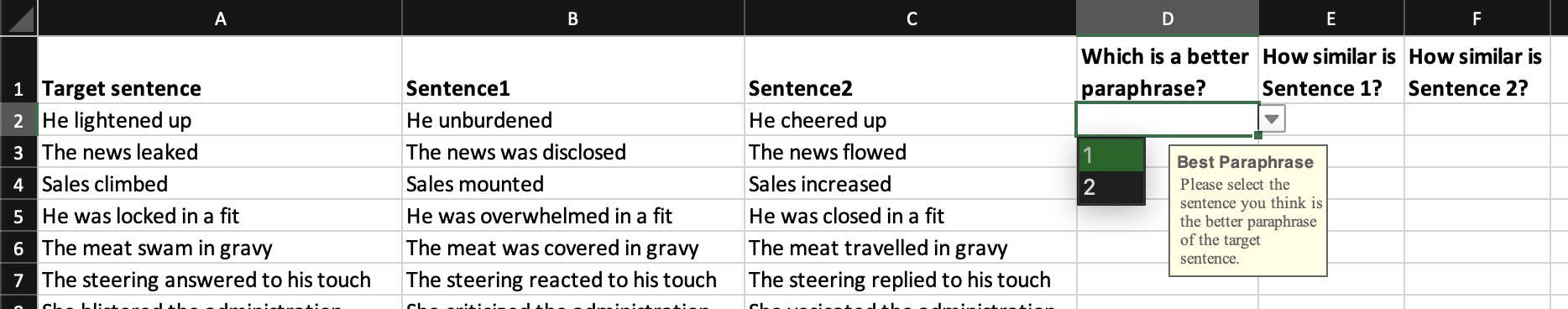
Figure 1: Participants are asked to choose which of paraphrase 1 or 2 is the best.

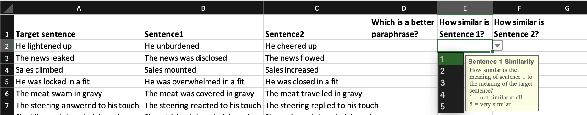
Figure 2: Participants are asked to rate the similarity of each paraphrase to the target sentence

Model Task

We evaluate a range of density matrix models, neural models, and baselines on this disambiguation task. The evaluation runs as follows. For each triple of sentences, we generate vectors or density matrices for each sentence. We then compute the similarity of the sentence representations using either cosine similarity (for vectors) or the generalized inner product (for density matrices. We assess the extent to which models agree with the mean of the human judgements using Spearman’s rho.

5.2 Models

We use the density matrices computed in [25]. We test 4 variants of Multi-sense Word2DM (ms-Word2DM). One parameter varies the number of senses computed for each matrix, either 5 or 10, and one varies the means by which the closest sense is chosen for updating, choosing the closest via cosine similarity (c) or by Euclidean distance (d).[25] also propose two other key ways of generating density matrices. One, called Context2DM, extends the methods proposed in [32, 37]. Firstly, a set of word vectors is trained with the gensim implementation of Word2Vec on the combined ukWaC+Wackypedia corpus. For each target word, the set of words whose context they appear in is collected. The vectors of these context words are clustered using hierarchical agglomerative clustering to between 2 and 10 clusters. The centroids of each of these clusters are taken to form the sense vectors for the target word, and subsequently these sense vectors are combined into a density matrix.

The second alternative method, Bert2DM uses BERT [15] to generate sense vectors. BERT is a Transformer-based architecture [40] which produces contextual embeddings, meaning that the vector produced for each word is dependent on the context of the sentence. A small corpus is fed through BERT. Vectors for each word are extracted, and dimensionality reduction applied (either PCA or SVD). Vectors for each word are then combined to form density matrices.

We compare performance with two neural sentence encoders, SBERT [34] and InferSent [12]. Both of these models are explicitly trained to predict when one sentence can be inferred from another. Since synonymy is a simple kind of entailment relation, these sentence encoders should perform well.

We compare with two baseline models, word2vec [26] and GloVe [31]. These are two methods for producing static word vectors with the key property that semantically similar words should be close together in the vector space.

6 Experiments and Results

For each model described in the previous section, we generate sentence embeddings for triples in the dataset. For the density matrix methods, we apply the composition methods outlined in 4.2, that is, Add, Mult, Fuzz, and Phaser. For neural methods, we simple take the sentence embeddings produced by the models. For the static word vector baselines, we apply Add and Mult. We also use a baseline ‘composition’ method of simply taking the verb as sentence representation (Verb only)

We compute $sim(\llbracket target\rrbracket,\llbracket apt\rrbracket)$ and $sim(\llbracket target\rrbracket,\llbracket inapt\rrbracket)$, where $sim$ is cosine similarity for vectors and generalized inner product for density matrices. We compare the similarity scores generated by the models to the similarity scores generated by humans and compute the correlation between these scores using Spearman’s rho. Spearman’s rho ranges between -1 and 1, with 1 indicating that scores are perfectly correlated and -1 indicating that they are perfectly anti-correlated.

For each model tested, there were a number of occurrences of words in the dataset that were not in the lexicon of the trained model. Where this occurred, the sentence pairs containing these words were removed from the tests for the given model. The error occurred more frequently with the long-form dataset due to words not being in their lemmatised form. For Context2DM and BERT2DM with the long-form dataset, the results were deemed unreliable and not included due to having only 8 usable sentence pairs. Table 6 in the Appendix shows the number of sentence pairs used in the tests, out of the total of 342 sentence pairs, as a result of these errors being removed.

6.1 Results

Results are shown in tables 1, 2 and 3. Table 1 shows firstly that the neural sentence encoders (left hand table) were not able to correctly interpret the metaphorically used word in context, with correlation close to 0, i.e. indicating chance level. Secondly, on the right hand side, we see that in the compositional settings (Add and Mult), static word vectors also perform poorly, although very slightly better than the sentence encoders. For the Verb-only setting, we see a stronger negative correlation, i.e., similarity ratings are more consistently in the wrong direction. This is expected, as the verb alone does not provide the context necessary for disambiguation of the metaphor, and we would expect that the most common sense of a word would dominate the learnt representations.

SBERT	short	-0.0317
	long	-0.0146
Infersent1	short	0.0085
	long	-0.0027
Infersent2	short	0.0113
	long	-0.0411

		Verb	Add	Mult
Word2Vec	short	-0.2719	-0.0536	-0.1092
	long		-0.0010	-0.0642
GloVe	short	-0.1529	-0.0272	0.0738
	long		0.0236	0.0579

-0.3

-0.2

-0.1

0

0.04

0.08

0.12

Table 1: Spearman’s rho for sentence encoders and vector baselines. Note that all sentence encoders performed poorly, while Glove with mult performed better.

In Table 2, we see a similar pattern. The verb-only baseline produces similarity ratings that are negatively correlated with those of humans. In general, the BERT2DM and Context2DM models produce slightly stronger results. The highest correlation is produced by Multi-sense Word2DM with 10 senses, using Euclidean distance to choose which sense to update, and using Mult as the composition operator. Overall, correlation is low. Table 3 gives performance of the density matrix models when using Fuzz or Phaser as the composition operator. When applying Fuzz and Phaser, there is a choice of whether to use the verb as the operator or the noun as the operator. The linguistically motivated choice is to use the verb as the operator. However, as seen in table 3, using the noun as the operator produces a better correlation with human judgements. We speculate that when using the verb as operator, the most common sense of the verb dominates the composition. In the case of a metaphorical verb, we require that the noun modifies the meaning of the verb to obtain the correct interpretation.

		Verb	Add	Mult
ms-Word2DM-c5	short	-0.2062	-0.0587	0.0201
	long		0.0373	-0.0764
ms-Word2DM-c10	short	-0.2094	-0.0552	-0.0365
	long		0.0450	-0.0577
ms-Word2DM-d5	short	-0.2519	-0.0999	-0.0204
	long		0.0136	0.0385
ms-Word2DM-d10	short	-0.2102	-0.0784	-0.0609
	long		0.0432	0.1061
Word2DM	short	-0.1772	-0.1063	-0.0004
	long		-0.0057	0.0263
bert2dm-pca-cls	short	0.0120	0.0749	0.0262
bert2dm-svd-cls	short	-0.0296	0.0172	0.0698
context2dm	short	0.0240	0.0483	0.0885

-0.3

-0.2

-0.1

0

0.04

0.08

0.12

Table 2: Spearman’s rho for density matrix models with simple composition. Most models with verb-only composition had negative correlation. ms-Word2DM-d10 with mult-long had the best performance.

All models except for BERT2DM-svd-cls and Context2DM consistently show an increase in rho after composition, supporting the idea that interpretation of metaphor is easier when provided with context.

	Fuzz verb	Fuzz noun	Phaser verb	Phaser noun
ms-Word2DM-c5	-0.1732	0.0378	-0.0251	0.0148
ms-Word2DM-c10	-0.1681	-0.0146	-0.0949	-0.0160
ms-Word2DM-d5	-0.1783	0.0576	-0.1132	0.0121
ms-Word2DM-d10	-0.1997	0.0402	-0.1552	-0.0125
Word2DM	-0.1042	-0.0008	-0.1311	-0.0029
bert2dm-pca-cls	0.0217	0.0274	0.0337	0.0186
bert2dm-svd-cls	-0.0280	0.0377	-0.0451	0.0358
context2dm	0.0177	0.0448	-0.0088	0.0350

-0.3

-0.2

-0.1

0

0.04

0.08

0.12

Table 3: Spearman’s rho for density matrix models with Fuzz and Phaser composition on the short-form dataset. Verb operator models generally had poor performance while noun operator models, especially with Fuzz, performed better.

6.2 Analysis

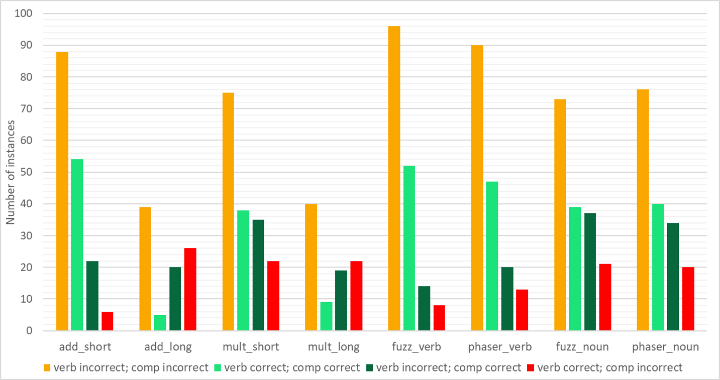
Figure 3: Analysis of which sentences were scored correctly by ms-Word2DM-d10. Note that verb operator models scored a lot of sentences the same as the verb, meaning composition had little effect.

To understand more about which sentences were being scored correctly, we examined the responses of ms-word2dm-d10. Each instance of a metaphorical sentence and its two paraphrases was marked correct if the apt paraphrase scored higher on cosine similarity than the inapt paraphrase, and incorrect if the inapt paraphrase scored highest. These results were then compiled for different composition methods and compared with the verb baseline. The number of instances correct and incorrect with verb and composition are shown in figure 3. We see that overall, the majority of similarity judgements are incorrect for verb-only models and for compositional models (yellow bar). We also see that for many models, both the verb-only and the compositional models are correct (light green bar). For Fuzz and Phaser, models where the verb is the operator showed fewer instances where the result changes after composition. This means that in more cases, the result remained either correct or incorrect according to the result of the verb alone. In contrast, the noun operator models had more instances where the verb-only model was incorrect and the composition was correct (dark green bar). This also indicates that the result is being heavily influenced by the operator matrix. Finally, there are a lot of instances where the verb-only model produces the correct answer but this is ‘undone’ by the composition (red bar). For Add and Mult, the long-form sentences showed a greater proportion of the correct sentences using the verb that became incorrect after composition, suggesting that the extra words in the long sentences may be distracting from the relevant information.

To analyse how each composition method affects the modelled ambiguity, we calculated the von Neumann entropy of each of the sentences for each composition method including the verb baseline, as shown in tables 4 and 5. The relative difference in entropy between the verb and the sentence embedding indicates the model’s change in ambiguity upon composition of the sentence. This is shown by the colour of the cells, red meaning an increase in entropy and blue meaning a decrease. The entropy results are consistent with the results for the similarity task; Phaser resulted in a greater reduction in entropy than Fuzz, and also produced stronger Spearman correlation. BERT2DM-svd-cls mult-short also had a high rho and a strong reduction in entropy.

		Verb	Add	Mult
ms-Word2DM-c5	short	1.1464	1.9298	1.6927
	long	1.1464	1.7579	1.8508
ms-Word2DM-c10	short	1.3230	2.2118	1.6821
	long	1.3230	1.9797	1.9587
ms-Word2DM-d5	short	1.0590	1.9834	1.4786
	long	1.0590	1.7171	1.6482
ms-Word2DM-d10	short	1.4508	2.1462	1.6160
	long	1.4508	2.0085	1.8854
Word2DM	short	0.1799	1.5876	0.9849
	long	0.1799	1.0555	0.4431
bert2dm-pca-cls	short	0.4647	1.0575	0.4467
bert2dm-svd-cls	short	0.2346	0.4943	0.0339
context2dm	short	0.2877	0.4546	0.3097

0.01

0.05

0.22

1

2.15

4.64

10

Table 4: Mean von Neumann entropy produced by density matrix models with simple composition. Colour indicates the relative change in entropy with composition. Bert2dm-svd-cls with mult is the only model to significantly decrease entropy.

	Verb	Fuzz verb	Fuzz noun	Phaser verb	Phaser noun
ms-Word2DM-c5	1.1464	0.6781	0.6731	0.3661	0.3550
ms-Word2DM-c10	1.3230	0.8769	0.9141	0.4971	0.4860
ms-Word2DM-d5	1.0590	0.7257	0.6873	0.3046	0.2798
ms-Word2DM-d10	1.4508	0.8580	0.8412	0.4034	0.3918
Word2DM	0.1799	0.2896	0.2519	0.0511	0.0413
bert2dm-pca-cls	0.4647	0.3001	0.3182	0.1245	0.1269
bert2dm-svd-cls	0.2346	0.0444	0.0546	0.0103	0.0103
context2dm	0.2877	0.0912	0.0389	0.0041	0.0041

0.01

0.05

0.22

1

2.15

4.64

10

Table 5: Mean von Neumann entropy produced by density matrix models with Fuzz and Phaser on short-form dataset. Colour indicates the relative change in entropy with composition. Note that Phaser caused a greater entropy reduction than Fuzz.

7 Discussion and Conclusions

Interpreting metaphor correctly is an essential part of language understanding. Previous work showed that density matrix approaches to modelling language meaning could effectively capture ambiguity. The aim of this paper was to test whether these representations could capture ambiguity in the case of conventional metaphor. We built a new dataset to test our models, and tested a range of density matrix word representations and composition methods, as well as neural sentence encoders. All models found this dataset extremely difficult. However, we do see some insights into how metaphor can be interpreted. Firstly, in almost all compositional methods, we see an increase in performance over a simple verb-only baseline. We also see some increases in performance over simple vector-based models. We find that using the non-metaphorical nouns as operators rather than the metaphorical verbs gives improved performance, indicating that perhaps we need to view the metaphorically used words as being updated by their context. We also see that in the case of Fuzz and Phaser composition, the composition reduces the entropy of representations, as previously seen in [32, 25]

Further Work

We have tested our dataset on SBERT and InferSent, however, recently, a wide range of language models have become available, and we plan to test those models on this difficult dataset. The work we have presented in this paper relates only to conventional metaphor, which can be seen fairly straightforwardly as a case of lexical ambiguity. Work is ongoing to extend these methods to novel metaphor, where new meanings must be created on-the-fly. Another line of enquiry is to link the interpretation of density matrices as modelling ambiguity with the interpretation as modelling hyponymy. The categorisation theory of metaphor proposed in [16] argues that in noun-noun metaphors (e.g. ‘My lawyer is a shark’), an ad-hoc class (e.g. ‘vicious things’) is created that abstracts both the metaphor and its target. We can therefore use the entailment interpretation of density matrices to discover these ad-hoc classes by finding something like a greatest lower bound for downward entailment – with the caveat that such bounds are not always unique for density matrices. There is potential to integrate these methods with the DiscoCirc formalism [8], in which a sense of narrative is included, and the level of modelling is at the full text rather than sentence level. Finally, implementing quantum-inspired models using real quantum computers is a burgeoning new line of research [24] and our methods have already been investigated in simulation in [7]. Pushing these ideas further will be an important step in this process.

Appendix A Numbers of Sentence Pairs

		Cosine Similarity	Von Neumann Entropy
GloVe	verb-only	331
	short-form	269
	long-form	63
Word2Vec	verb-only	331
	short-form	269
	long-form	63
BERT2DM models	verb-only	300	336
	short-form	204	252
	long-form	8	10
Context2DM	verb-only	310	338
	short-form	212	256
	long-form	8	10
Word2DM models	verb-only	332	342
	short-form	335	342
	long-form	172	220

Table 6: Number of sentence pairs used in each test after removing out-of-vocabulary words. SBERT and Infersent covered all words.

References

- [1]
- [2] Esma Balkır, Mehrnoosh Sadrzadeh & Bob Coecke (2016): Distributional Sentence Entailment Using Density Matrices. In Mohammad T. Hajiaghayi & Mohammad R. Mousavi, editors: Topics in Theoretical Computer Science, Lecture Notes in Computer Science 9541, Springer, Cham, pp. 1–22. Available at https://doi.org/10.1007/978-3-319-28678-5_1.
- [3] Dea Bankova, Bob Coecke, Martha Lewis & Dan Marsden (2019): Graded Hyponymy for Compositional Distributional Semantics. Journal of Language Modelling 6(2), p. 225, 10.15398/jlm.v6i2.230. Available at http://jlm.ipipan.waw.pl/index.php/JLM/article/view/230.
- [4] Marco Baroni & Roberto Zamparelli (2010): Nouns are Vectors, Adjectives are Matrices: Representing Adjective-Noun Constructions in Semantic Space. In: Proceedings of the 2010 Conference on Empirical Methods in Natural Language Processing, Association for Computational Linguistics, pp. 1183–1193. Available at https://dl.acm.org/doi/abs/10.5555/1870658.1870773.
- [5] William Blacoe, Elham Kashefi & Mirella Lapata (2013): A Quantum-Theoretic Approach to Distributional Semantics. In: Proceedings of the 2013 Conference of the North American Chapter of the Association for Computational Linguistics: Human Language Technologies, Association for Computational Linguistics, Atlanta, Georgia, pp. 847–857. Available at https://aclanthology.org/N13-1105.
- [6] Tai-Danae Bradley & Yiannis Vlassopoulos (2021): Language Modeling with Reduced Densities. Compositionality 3, p. 4. Available at https://doi.org/10.32408/compositionality-3-4.
- [7] Saskia Bruhn (2021): Density Matrix Methods in Quantum Natural Language Processing. Ph.D. thesis, Master’s thesis, Universität Osnabrück, 2022. doi: 10.48693/111.
- [8] Bob Coecke (2021): The mathematics of text structure. Joachim Lambek: The Interplay of Mathematics, Logic, and Linguistics, pp. 181–217. Available at https://doi.org/10.48550/arXiv.1904.03478.
- [9] Bob Coecke & Konstantinos Meichanetzidis (2020): Meaning Updating of Density Matrices. Journal of Applied Logics 2631(5), p. 745. Available at https://doi.org/10.48550/arXiv.2001.00862.
- [10] Bob Coecke & Éric Oliver Paquette (2011): Categories for the practising physicist. In: New Structures for Physics, Springer, pp. 173–286. Available at https://doi.org/10.1007/978-3-642-12821-9_3.
- [11] Bob Coecke, Mehrnoosh Sadrzadeh & Stephen J Clark (2010): Mathematical Foundations for a Compositional Distributional Model of Meaning. Linguistic Analysis 36(1), pp. 345–384. Available at https://doi.org/10.48550/arXiv.1003.4394.
- [12] Alexis Conneau, Douwe Kiela, Holger Schwenk, Loïc Barrault & Antoine Bordes (2017): Supervised Learning of Universal Sentence Representations from Natural Language Inference Data. In: Proceedings of the 2017 Conference on Empirical Methods in Natural Language Processing, pp. 670–680, 10.18653/v1/D17-1070.
- [13] Adriana D. Correia, Michael Moortgat & Henk T. C. Stoof (2020): Density Matrices with Metric for Derivational Ambiguity, 10.48550/arXiv.1908.07347. Available at http://arxiv.org/abs/1908.07347.
- [14] Gemma De las Cuevas, Andreas Klingler, Martha Lewis & Tim Netzer (2020): Cats Climb Entails Mammals Move: Preserving Hyponymy in Compositional Distributional Semantics. arXiv:2005.14134 [cs, math]. Available at https://doi.org/10.48550/arXiv.2005.14134.
- [15] Jacob Devlin, Ming-Wei Chang, Kenton Lee & Kristina Toutanova (2019): BERT: Pre-training of Deep Bidirectional Transformers for Language Understanding. In Jill Burstein, Christy Doran & Thamar Solorio, editors: Proceedings of the 2019 Conference of the North American Chapter of the Association for Computational Linguistics: Human Language Technologies, Volume 1 (Long and Short Papers), Association for Computational Linguistics, Minneapolis, Minnesota, pp. 4171–4186, 10.18653/v1/N19-1423. Available at https://aclanthology.org/N19-1423.
- [16] Sam Glucksberg & Boaz Keysar (1990): Understanding metaphorical comparisons: Beyond similarity. Psychological review 97(1), p. 3. Available at https://doi.org/10.1037/0033-295X.97.1.3.
- [17] Dimitri Kartsaklis (2015): Compositional Distributional Semantics with Compact Closed Categories and Frobenius Algebras. Ph.D. thesis, University of Oxford. Available at https://arxiv.org/abs/1505.00138.
- [18] Dimitri Kartsaklis, Matthew Purver & Mehrnoosh Sadrzadeh (2016): Verb Phrase Ellipsis using Frobenius Algebras in Categorical Compositional Distributional Semantics. In: DSALT Workshop, European Summer School on Logic, Language and Information, pp. 1–2. Available at https://www.eecs.qmul.ac.uk/~mpurver/papers/kartsaklis-et-al16dsalt.pdf.
- [19] Germán Kruszewski, Denis Paperno, Raffaella Bernardi & Marco Baroni (2016): There Is No Logical Negation Here, But There Are Alternatives: Modeling Conversational Negation with Distributional Semantics. Computational Linguistics 42(4), pp. 637–660, 10.1162/COLI_a_00262. Available at https://aclanthology.org/J16-4003.
- [20] Joachim Lambek (1997): Type Grammar Revisited. In Alain Lecomte, François Lamarche & Guy Perrier, editors: Logical Aspects of Computational Linguistics, Second International Conference, LACL ’97, Nancy, France, September 22-24, 1997, Selected Papers, Lecture Notes in Computer Science 1582, Springer, pp. 1–27. Available at https://doi.org/10.1007/3-540-48975-4_1.
- [21] Michael Lesk (1986): Automatic sense disambiguation using machine readable dictionaries: how to tell a pine cone from an ice cream cone. In: Proceedings of the 5th annual international conference on Systems documentation, SIGDOC ’86, Association for Computing Machinery, New York, NY, USA, pp. 24–26, 10.1145/318723.318728. Available at https://dl.acm.org/doi/10.1145/318723.318728.
- [22] Martha Lewis (2019): Compositional Hyponymy with Positive Operators. In: Proceedings of the International Conference on Recent Advances in Natural Language Processing (RANLP 2019), INCOMA Ltd., Varna, Bulgaria, pp. 638–647, 10.26615/978-954-452-056-4_075. Available at https://www.aclweb.org/anthology/R19-1075.
- [23] Martha Lewis (2020): Towards Logical Negation for Compositional Distributional Semantics. IfCoLog Journal of Applied Logics 7(5), pp. 771–794. Available at https://doi.org/10.48550/arXiv.2005.04929.
- [24] Robin Lorenz, Anna Pearson, Konstantinos Meichanetzidis, Dimitri Kartsaklis & Bob Coecke (2023): QNLP in practice: Running compositional models of meaning on a quantum computer. Journal of Artificial Intelligence Research 76, pp. 1305–1342, 10.1613/jair.1.14329.
- [25] Francois Meyer & Martha Lewis (2020): Modelling Lexical Ambiguity with Density Matrices. In: Proceedings of the 24th Conference on Computational Natural Language Learning, Association for Computational Linguistics, Online, pp. 276–290, 10.18653/v1/2020.conll-1.21. Available at https://www.aclweb.org/anthology/2020.conll-1.21.
- [26] Tomas Mikolov, Ilya Sutskever, Kai Chen, Greg S Corrado & Jeff Dean (2013): Distributed representations of words and phrases and their compositionality. Advances in neural information processing systems 26. Available at https://doi.org/10.48550/arXiv.1310.4546.
- [27] George A. Miller (1995): WordNet: A Lexical Database for English. Communinications of the ACM 38(11), pp. 39–41. Available at http://doi.acm.org/10.1145/219717.219748.
- [28] Jeff Mitchell & Mirella Lapata (2010): Composition in Distributional Models of Semantics. Cognitive Science 34(8), pp. 1388–1429, 10.1111/j.1551-6709.2010.01106.x. Available at https://onlinelibrary.wiley.com/doi/abs/10.1111/j.1551-6709.2010.01106.x.
- [29] Saif Mohammad, Ekaterina Shutova & Peter Turney (2016): Metaphor as a medium for emotion: An empirical study. In: Proceedings of the Fifth Joint Conference on Lexical and Computational Semantics, pp. 23–33, 10.18653/v1/S16-2003.
- [30] Roberto Navigli (2009): Word sense disambiguation: A survey. ACM computing surveys (CSUR) 41(2), pp. 1–69. Available at https://doi.org/10.1145/1459352.1459355.
- [31] Jeffrey Pennington, Richard Socher & Christopher D Manning (2014): Glove: Global vectors for word representation. In: Proceedings of the 2014 conference on empirical methods in natural language processing (EMNLP), pp. 1532–1543, 10.3115/v1/D14-1162.
- [32] Robin Piedeleu, Dimitri Kartsaklis, Bob Coecke & Mehrnoosh Sadrzadeh (2015): Open System Categorical Quantum Semantics in Natural Language Processing. In Lawrence S. Moss & Pawel Soboci’nski, editors: 6th Conference on Algebra and Coalgebra in Computer Science, CALCO 2015, June 24-26, 2015, Nijmegen, The Netherlands, LIPIcs 35, Schloss Dagstuhl - Leibniz-Zentrum fuer Informatik, pp. 270–289. Available at https://doi.org/10.4230/LIPIcs.CALCO.2015.270.
- [33] Anne Preller & Mehrnoosh Sadrzadeh (2011): Bell States and Negative Sentences in the Distributed Model of Meaning. Electronic Notes in Theoretical Computer Science 270(2), pp. 141 – 153. Available at https://doi.org/10.1016/j.entcs.2011.01.028. Proceedings of the 6th International Workshop on Quantum Physics and Logic (QPL 2009).
- [34] Nils Reimers & Iryna Gurevych (2019): Sentence-BERT: Sentence Embeddings using Siamese BERT-Networks. In: Proceedings of the 2019 Conference on Empirical Methods in Natural Language Processing and the 9th International Joint Conference on Natural Language Processing (EMNLP-IJCNLP), pp. 3982–3992, 10.18653/v1/D19-1410.
- [35] Benjamin Rodatz, Razin Shaikh & Lia Yeh (2021): Conversational Negation Using Worldly Context in Compositional Distributional Semantics. In: Proceedings of the 2021 Workshop on Semantic Spaces at the Intersection of NLP, Physics, and Cognitive Science (SemSpace), Association for Computational Linguistics, Groningen, The Netherlands, pp. 53–65. Available at https://doi.org/10.48550/arXiv.2105.05748.
- [36] Mehrnoosh Sadrzadeh, Dimitri Kartsaklis & Esma Balkır (2018): Sentence Entailment in Compositional Distributional Semantics. Annals of Mathematics and Artificial Intelligence 82(4), pp. 189–218. Available at https://doi.org/10.1007/s10472-017-9570-x.
- [37] Hinrich Schütze (1998): Automatic Word Sense Discrimination. Comput. Linguist. 24(1), pp. 97–123. Available at https://dl.acm.org/doi/10.5555/972719.972724.
- [38] Peter Selinger (2007): Dagger Compact Closed Categories and Completely Positive Maps: (Extended Abstract). Electronic Notes in Theoretical Computer Science 170, pp. 139 – 163. Available at https://doi.org/10.1016/j.entcs.2006.12.018. Proceedings of the 3rd International Workshop on Quantum Programming Languages (QPL 2005).
- [39] Razin A. Shaikh, Lia Yeh, Benjamin Rodatz & Bob Coecke (2022): Composing Conversational Negation. Electronic Proceedings in Theoretical Computer Science 372, p. 352–367. Available at http://dx.doi.org/10.4204/EPTCS.372.25.
- [40] Ashish Vaswani, Noam Shazeer, Niki Parmar, Jakob Uszkoreit, Llion Jones, Aidan N Gomez, Łukasz Kaiser & Illia Polosukhin (2017): Attention is all you need. Advances in neural information processing systems 30. Available at https://doi.org/10.48550/arXiv.1706.03762.
- [41] John van de Wetering (2017): Ordering information on distributions. arXiv:1701.06924.