Efficient Exploration and Discriminative World Model Learning with an Object-Centric Abstraction

Abstract

In the face of difficult exploration problems in reinforcement learning, we study whether giving an agent an object-centric mapping (describing a set of items and their attributes) allow for more efficient learning. We found this problem is best solved hierarchically by modelling items at a higher level of state abstraction to pixels, and attribute change at a higher level of temporal abstraction to primitive actions. This abstraction simplifies the transition dynamic by making specific future states easier to predict. We make use of this to propose a fully model-based algorithm that learns a discriminative world model, plans to explore efficiently with only a count-based intrinsic reward, and can subsequently plan to reach any discovered (abstract) states.

We demonstrate the model’s ability to (i) efficiently solve single tasks, (ii) transfer zero-shot and few-shot across item types and environments, and (iii) plan across long horizons. Across a suite of 2D crafting and MiniHack environments, we empirically show our model significantly out-performs state-of-the-art low-level methods (without abstraction), as well as performant model-free and model-based methods using the same abstraction. Finally, we show how to reinforce learn low level object-perturbing policies, as well as supervise learn the object mapping itself.

1 Introduction

Since the inception of reinforcement learning (RL), the problems of exploration and world model learning have been major roadblocks. RL requires an agent to learn both basic motor abilities, and explore long sequences of interactions in the environment. Currently, we have made tremendous progress on problems of low-level control for short-horizon problems. With well defined single tasks, given enough samples (or demonstrations), there are well-developed ways of training low level policies reliably (Schulman et al.,, 2017; Hafner et al.,, 2023).

Perhaps a better way to explore complex environments is to treat the high-level exploration problem separately. We increasingly have the ability to get semantically rich abstractions: via representation learning (Locatello et al.,, 2020), object segmentation (Kirillov et al.,, 2023), and visual-language models  (Alayrac et al.,, 2022); even in difficult control settings such as robotics (Liu et al.,, 2024). In addition, with the recent explosion in the field of natural language processing, people are increasingly interested in addressing RL environments on a semantic level (Andreas et al.,, 2017; Jiang et al.,, 2019; Chen et al.,, 2021). Thus, we ask a timely question: if the agent has a good ability to perceive objects, what more can we do other than tabula rasa learning at the level of pixels and primitive motor actions?

In this work, we focus on exploration and world modelling at a semantic level. We explore a simple yet flexible abstraction: in addition to the agent’s raw observations (e.g. pixels), it sees an abstract representation of a set of items and their attributes (i.e. object states). We find that to navigate these two levels effectively, it is best to construct a proxy decision process (Ab-MDP) with state and temporal abstractions at the level of objects, with a handful of competent object-perturbing low level policies. By construction, dynamics on this semantic level becomes structured, and we make use of this to design a discriminative model-based RL method that learns to predicts if a specific object perturbation will be successful. Our method, Model-based Exploration of abstracted Attribute Dynamics (MEAD), is fit with a simple objective to model semantic level transitions, resulting in stable model improvements with no need for auxiliary objectives. It is fully online: the agent plans to explore without an extrinsic reward to learn about the world it inhabits using a count-based objective. The same model can be used at any point to plan to solve downstream tasks when given a goal function, without the need to train policy or value functions.

The main results of this work investigates decision making at the semantic level as defined by the Ab-MDP, assuming access to an object centric map and object perturbing policies. We empirically evaluate our method in a set of 2D crafting games, and MiniHack environments that are known to be very difficult to explore (Henaff et al.,, 2022). We then show how to learn components of the Ab-MDP when it is not given: by reinforcement learning object perturbation policies given an object mapping, and supervised learning of the object centric mapping itself.

The main contributions of this work are:

• We define the Ab-MDP: a simple human-understandable hierarchical MDP. The structure of this abstraction allows for pre-trained or from-scratch visual encoders to be used. It also allows our method (MEAD) to use a discriminative objective for world-model learning.

• We introduce our model-learning method (MEAD). MEAD uses a stable discriminative objective to model item attribute changes, which is more efficient at learning than generative-based baselines and also allows for efficient inference-time planning.

• We empirically show MEAD extracts an interpretable world model, accurately plans over long horizons, reaches competitive final performance on all levels with greater sample efficiency to strong baselines, and transfers well to new environments.

• We demonstrate how to learn parts of the Ab-MDP when it is not given: by reinforcement learning object-perturbing policies, and supervised learning the object-centric mapping.

2 Problem Setting

We begin by considering a (reward free) “base” Markov Decision Process (MDP) as the tuple $\langle\mathcal{S},\mathcal{A},P\rangle$, with state space $\mathcal{S}$, primitive action space $\mathcal{A}$, and transition probability function $P:\mathcal{S}\times\mathcal{A}\times\mathcal{S}\rightarrow[0,1]$ (Puterman,, 1994). Below we construct the “abstracted” space.

2.1 Abstract states and behaviours

We give the agent a deterministic object-centric mapping $\text{M}\!\!:\mathcal{S}\rightarrow\mathcal{X}$ from low level observations to an abstract state $X\in\mathcal{X}$. The abstract state is a discrete set of items, each having form (item identity, item attribute). Denote the $i$-th item in this (ordered) set as $x^{(i)}$, each $x^{(i)}=(\alpha^{(i)},\xi^{(i)})$ consists of an item’s identity $\alpha^{(i)}$ (e.g. “potion”), and attribute $\xi^{(i)}$ (e.g. “in inventory”). In practice, each $X$ is represented as a $N\times(d_{\text{iden}}+d_{\text{attr}})$ matrix containing $N$ items (including empty items) each having a $d_{\text{iden}}$ dimensional identity embedding and $d_{\text{attr}}$ dimensional attribute embedding.

Denote a space $\mathcal{B}$ of object perturbation policies which we call behaviours. Each behaviour has an associated $\pi_{b}:\mathcal{S}\rightarrow\mathcal{A}$. A behaviour $b=(\alpha^{(i)},\xi^{\prime})$ describes a single item id $\alpha^{(i)}$ and a desired new attribute. For $N$ objects and $m$ attributes, there are $N\times m$ single item behaviours. Not all behaviours changes $\alpha^{(i)}$ to have $\xi^{\prime}$ (due to the change being impossible from current $X$, or having a bad $\pi_{b}$). A behaviour is competent if executing behaviour policy $\pi_{b}$ from state $S,\,\text{M}(S)=X$, result in arriving at state $S^{\prime},\,\text{M}(S^{\prime})=X^{\prime}$, $(\alpha^{(i)},\xi^{\prime})\in X^{\prime}$, within $k$ steps with high probability. See Appendix B.1 for more details. Executing competent behaviours lead to predictable changes.

For the main experiments we assume access to (learned or given) abstract states and behaviours and build on top. We address learning both in Section 4.3.

2.2 Abstracted Item-Attribute MDP

We now define an Abstracted Item-Attribute MDP using the abstract state $\mathcal{X}$ and behaviour $\mathcal{B}$ spaces, which we refer to in brief as Ab-MDP. The abstract mapping M provides an state abstraction. We further define the Ab-MDP to have a coarser temporal resolution than the low level MDP: an abstract transition only occurs when an abstract state changes, or if the state stays the same but $k$ low level steps elapses (see Definition B.1 for more details).

Specifically, the Ab-MDP is the tuple $\langle\mathcal{X},\mathcal{B},\textbf{T}\rangle$, with abstract states $\mathcal{X}$, abstract behaviours $\mathcal{B}$, and transition probability function $\textbf{T}:\mathcal{X}\times\mathcal{B}\times\mathcal{X}\rightarrow[0,1]$. $\textbf{T}(X^{\prime}|X,b)$ describes the probability of being in abstract state $X^{\prime}$ when starting from $X$, executing behaviour $b$, and waiting until an abstract transition occurs. Figure 1 provides an example of an abstract transition and associated low level steps. The Ab-MDP can be interpreted as Options (Sutton et al.,, 1999; Precup,, 2000), which we discuss in Appendix B.1.1.

There is an intuitive relationship between the competence of a behaviour and the transition probability function T. For instance, executing an incompetent behaviour $b$ from abstract state $X$ will likely lead to the next abstract state being itself, $X_{t+1}=X_{t}$, or some hard-to-predict distribution over next states. Executing a competent behaviour $b$ lead to a predictable next state that contains the proposed attribute change with high probability.

In any case, we can treat the Ab-MDP as a regular MDP use standard RL algorithms to solve it. This can be viewed as solving a proxy problem of the low level base MDP. For the remainder of this paper, all methods are trained exclusively within the Ab-MDP unless stated otherwise.

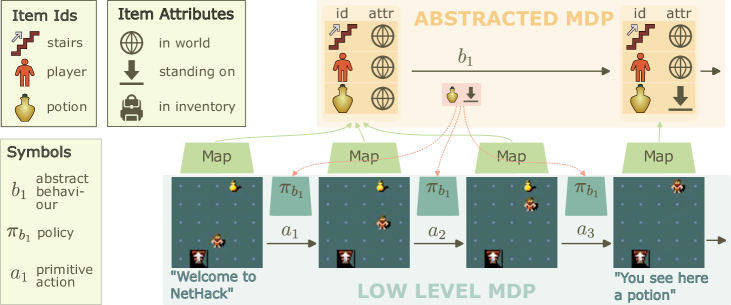
Figure 1: An example state transition in an Ab-MDP (here defined in MiniHack). Abstract states are sets of (item identity, item attribute), and behaviour $b_{1}$ have structure (item, new attribute). An abstract state can correspond to multiple low level states, and an abstract behaviour multiple primitive actions. We provide legends for the item identities and attributes illustrated (left rectangles).

3 Methods

While any standard RL methods can be used to solve the Ab-MDP, we develop a method to more fully make use of the item-attribute structure and item-perturbing behaviours. Specifically, we design a model-based method that efficiently explores and learn an accurate full world model. Our method, Model-based Exploration of abstracted Attribute Dynamics (MEAD) can be broken down into three components: (i) A forward model $f_{\theta}(X,b)$, (ii) A reward function $r(X,b)$, (iii) A planner which maximizes the reward function.

Our forward model takes in the current abstract state $X$ and behaviour $b$, and predicts the probability of success of the change proposed by the abstract behaviour. We describe the procedure for training the forward model in Section 3.1.

We use a different reward function and planner at training versus inference time. During training, the agent learns an accurate (abstract) world model without rewards. We use an intrinsic reward function $r_{\text{intr}}(X,b)$ that encourages infrequently visited states, and plan using Monte-Carlo Tree Search (MCTS) toward these states. Section 3.2 describes the exploration phase in detail.

At inference time, our aim is to reach a particular abstract state. We define our reward function $r_{\text{goal}}$ as $1$ for the goal abstract states and $0$ for all others. Because our forward model has been trained to accurately estimate state transitions, we simply run Dijkstra’s algorithm using $f_{\theta}$ and $r_{\text{goal}}$ to maximize expected reward. Section 3.3 describes this.

3.1 Forward model

A forward model takes in a current abstract state and behaviour to model the distribution over next states, $X_{t+1}\sim p(X_{t+1}|X_{t},b_{t})$. Typically, this distribution has support over the full state space $\mathcal{X}$. We observe that by construction, Ab-MDP considers competent policies as ones that change single item-attributes. Thus, we make the modelling assumption that an abstract transition would result in either (i) a single object’s attribute changing (as specified by the executed behaviour), or (ii) the abstract state remaining unchanged. It is of course possible for multiple items’ attributes to change at once, or for an unexpected item’s attribute to change—we show with a competent set of policies and re-planning our model is robust to this in practice in Appendix B.2.2.

Discriminative modelling

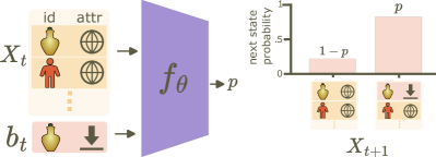
Figure 2: The forward model $f_{\theta}$ predicts the probability $p$ that the behaviour $b_{t}$ is successful from state $X_{t}$. The next state distribution is modelled as a binary distribution (Equation 3).

Given an abstract transition $(X_{t},b_{t},X_{t+1})$, we consider this transition successful if the next abstract state contains the attribute change proposed by the behaviour: $(\alpha^{(i)},\xi^{\prime})\in X_{t+1}$ for $b_{t}=(\alpha^{(i)},\xi^{\prime})$. Executing a competent policy has a high probability of leading to a successful transition.

We model this success probability directly,

$$q(X_{t}, b_{t})=\Pr(x^{\prime}\in X_{t+1}|X_{t},b_{t})\,,$$ (1)

$$\text{where }x^{\prime}=b_{t}=(\alpha^{(i)},\xi^{\prime})\,.$$

We refer to this way of modelling as discriminative world modelling, which models the probability that the state change specified by a behaviour is successful. As behaviours are by construction item perturbations, we can view this as asking a question about allowable item changes (“can I change this item to have this attribute?”). This is different from generative world modelling which models $\Pr(X_{t+1}|X_{t},b_{t})$ without any restrictions on possible future states (i.e. “what are all possible outcomes of my action in this state”). We find this inductive bias leads to more data efficient learning and multi-step planning (Section 4.4.1).

Forward Prediction

We can model the next state after a successful transition as,

$$X^{\prime}=\Delta(X,b)=X\setminus x^{(i)}\cup(\alpha^{(i)},\xi^{\prime})\,,\quad\text{for any }b=(\alpha^{(i)},\xi^{\prime})\,.$$ (2)

Then, given success probability function $q$ (Equation 1), we model the next state distribution as:

$$\Pr(X_{t+1}|X_{t},b_{t})=\begin{cases}\Delta(X_{t},b_{t})\,&\text{with probability }q(X_{t},b_{t})\,,\\ X_{t}&\text{with probability }1-q(X_{t},b_{t})\,.\end{cases}$$ (3)

See Figure 2 for an example. As mentioned above, our model is robust to cases where multiple items change through re-planning (Appendix B.2.2).

Model Learning

We use model function class $f_{\theta}:\mathcal{X}\times\mathcal{B}\rightarrow[0,1]$ with trainbale parameters $\theta$, and fit it to approximate success probability (Equation 1). We can estimate the empirical success probability from a dataset of trajectories simply by counting, and fit a binary cross entropy loss. We found this to be a stable, simple-to-optimize objective. More details in Appendix C.1.

3.2 Planning for exploration

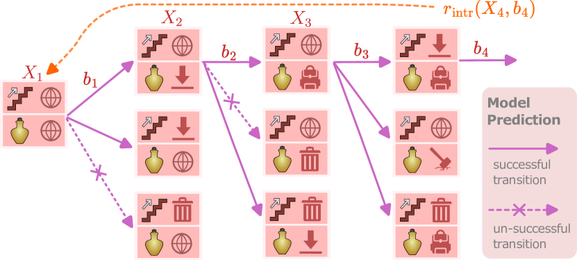
(a) Task agnostic training using MCTS and a count based reward to explore and learn the world model

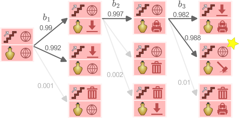
(b) Dijkstra planning at evaluation time to maximize success probability of reaching any goal state

Figure 3: Planning within model’s imagination to both explore, and to reach any goal state.

We want the agent to explore indefinitely to discover how the world works and represent it in its model $f_{\theta}$. We use a count-based intrinsic reward introduced in Zhang et al., (2018) which encourages the agent to uniformly cover all state-behaviours (details in Appendix C.3):

$$r_{\text{intr}}(X,b)=\sqrt{T/\left(\text{N}(X,b)+\epsilon T\right)}\,,$$ (4)

where $\text{N}(X,b)$ is a count of the number of times $(X,b)$ is visited, $T$ is the total number of (abstract) time-steps, and $\epsilon=0.001$ a smoothing constant.

We use Monte-Carlo Tree Search (MCTS) to find behaviours to reach states that maximizes Equation 4. This is done within the partially learned model’s imagination and allow the agent to plan toward novel states multiple steps in the future. The agent takes the first behaviour proposed. Further, since behaviours do not always succeed, one needs multiple state-visitations to estimate $q(X,b)$ well. We found MCTS exploration discovers more novel transition than exploring randomly (Section 4.4.2).

3.3 Planning for goal

Once the agent has sufficiently explored the environment and is well-fitted, the model $f_{\theta}$ usually contains a small set of high success probability edges between abstract states (see Figure 3(b); most item-attribute changes are generally impossible). We can use this model $f_{\theta}$ to plan to reach any desired (abstract) world state. As our model is not trained to maximize external rewards, we simply give it a function that tells it when it is in a desired state: $r_{\text{goal}}(X)=1\,\text{if }X\text{ is a goal state, and }0\text{ otherwise}$.

We use Dijkstra’s algorithm which finds the shortest path in a weighted graph. We turn our world model into a graph weighted by success probabilities, using a negative log transform:

$$d\!\left(X,\Delta(X,b)\right)=-\log f_{\theta}(X,b)\,,\quad\text{ with $\Delta(X,b)$ defined in Equation~{}\ref{eq:next-X-if-success}.}$$ (5)

Thus, finding the shortest path between current and goal state returns an abstract behaviour sequences that maximizes the probability of successfully reaching the goal.

4 Results

We use two sets of of environment. One is 2D crafting, which requires agent to craft objects following a Minecraft-like crafting tree with each crafting stage requiring multiple low level actions (Chen et al.,, 2020). Second is MiniHack (Samvelyan et al.,, 2021), which contains a series of extremely difficult exploration games (Henaff et al.,, 2022). We detail the environments further in Appendix D.

For baselines, we use strong model-free (asynch PPO, (Schulman et al.,, 2017; Petrenko et al.,, 2020)) and model-based (Dreamer-v3, (Hafner et al.,, 2023; Sekar et al.,, 2020)) baselines. More details in Appendix E. All the methods are trained in the Ab-MDP. We report low level steps and plot 95 confidence interval. See Appendix G for other experimental details.

4.1 Learning from scratch in single environments

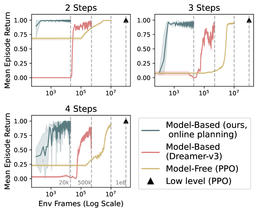
(a) 2D crafting games

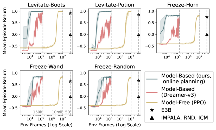
(b) MiniHack skill games

Figure 4: Results in games trained from scratch in Ab-MDP. Triangles and stars denote low-level only methods. For MiniHack, we also show the final performance of state-of-the-art exploration methods in the low level MDP (star/triangle), from Henaff et al., (2022). X-axis on log scale.

Figure 4 shows the from-scratch Ab-MDP training results for strong baselines and our method. We see that Dreamer-v3, a state-of-the-art model-based method, is highly sample efficient. PPO, a model-free method, stably optimizes the reward, but at a data budget of more than two orders of magnitude (hundreds of thousands versus 10 million). Our method learns the Ab-MDP with an additional order of magnitude sample efficiency improvement compared to the already efficient Dreamer. We also refer the reader to Figure 3(b) (which is a clean illustration of the same data presented in Appendix F.6) for an example of the interpretable world model we can extract from MEAD.

For reference, we plot the performance for SOTA algorithms in the base MDP (without the Ab-MDP) as triangles and stars. In particular in MiniHack tasks (Fig.4(b)), model-free methods with random and global exploration bonuses (IMPALA, RND, ICM) perform poorly even after 50 million steps, and methods using episodic exploration bonus perform better (E3B). Nonetheless, all of them are less efficient than the least efficient method trained on the Ab-MDP.

These results show that Ab-MDP helps simplify the problem, with all methods reaching reasonable performances—a feat not achievable by most methods trained in the low level MiniHack MDP (Henaff et al.,, 2022). However, we also see that the problem is still non-trivial, with the model-free baseline still requiring millions of frames to achieve success. Our method reaches the same peak performance as the model-free method while using fewer samples than the model-based baseline.

4.2 Transfer and Compositions

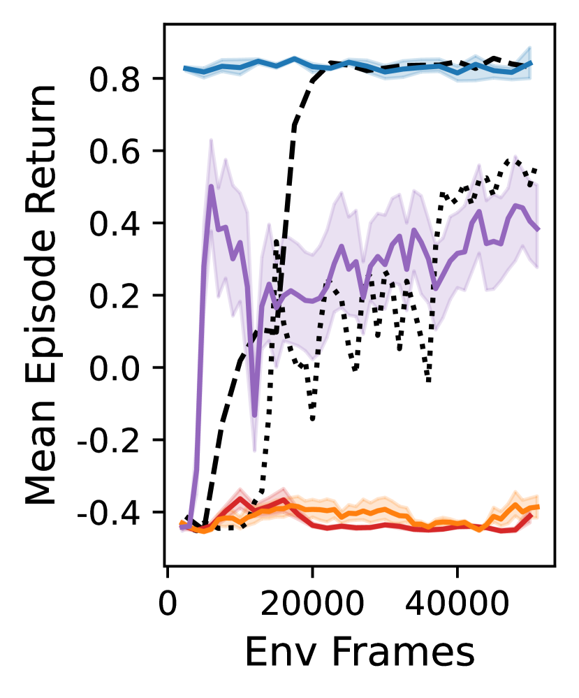
(a) Sandbox

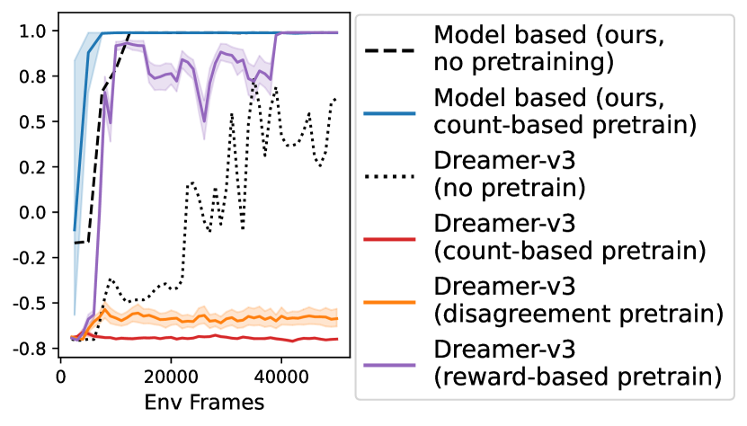
(b) Freeze-Random transfer

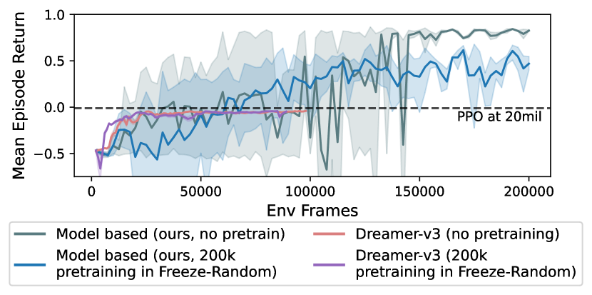
(c) Compositional environment.

Figure 5: Transfer experiments and a difficult compositional environment.

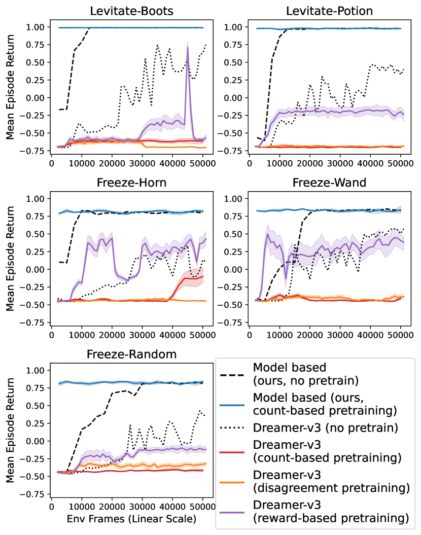
(a) Sandbox transfer performance. Episode return from fine-tuning model weights from pre-training in a sandbox environment containing multiple objects instances and types.

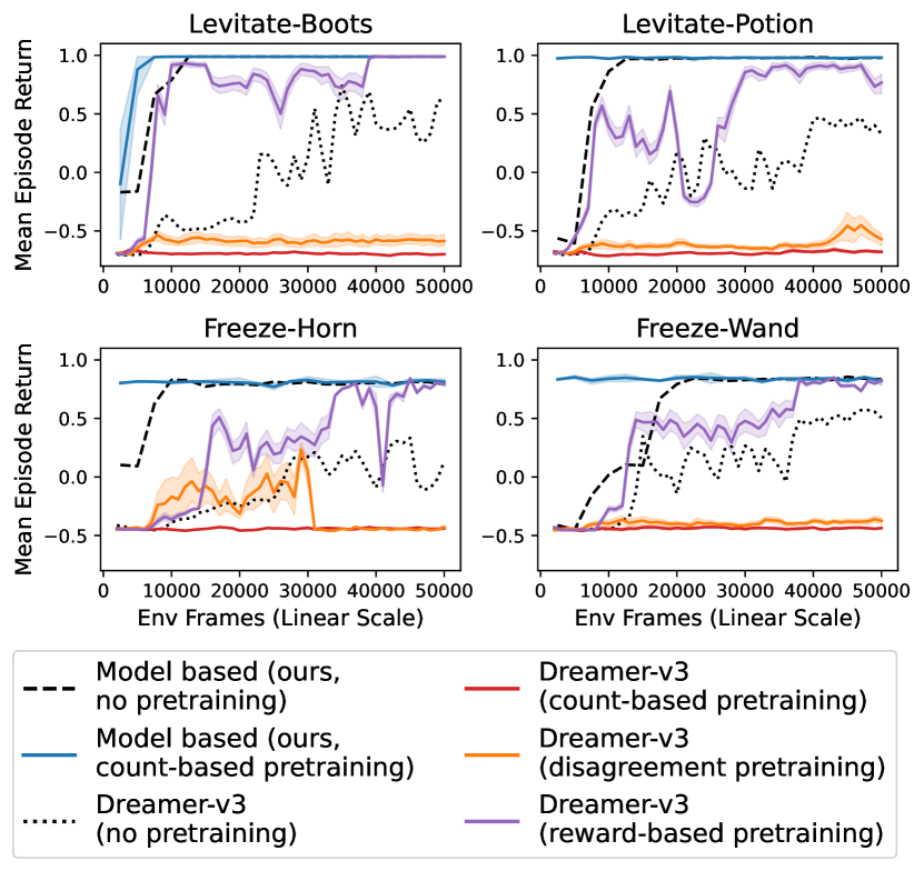
(b) Transfer to new object types. Pretrained in Freeze Random environment where Freeze Horn and Freeze Wand objects appear with 0.5 probabilities, fine-tuning on remaining 4 environments. (Top row): fine-tuning performance where new object type is fully unseen, (bottom row): fine-tuning performance for seen objects but appearing in different frequencies.

Figure 16: Full transfer experiments

Next, since the Ab-MDP abstraction models object identities and shared attributes, we evaluate if the abstract level models can transfer object knowledge to new settings. Here we exclusively use the MiniHack environments due to their rich repertoire of object types and higher difficulty. Note we run each transfer experiments in multiple environments; as the result is similar, we report a single illustrative environment in Figure 5 for brevity and provide full results in the Appendix Figure 16.

Sandbox transfer

We first place the agent in a “sandbox” environment where all objects are spawned with some probability (Appendix D.2.1). The agent is allowed to interact with the environment with only an exploration reward (no task-specific reward) for 200k frames. We then fine-tune the agent in each of the environments. For our model, we continue to train $f_{\theta}$ within the new environment. For Dreamer-v3, we transfer only the world model (encoder, decoder and dynamics function) and re-initialize the policy and reward functions. Results for all five environments follow similar trends, thus we show a representative example in Figure 5(a) and present the full set in Figure 16(a).

Surprisingly, Dreamer-v3 trained with both count- and disagreement-based intrinsic rewards fails to get any meaningful rewards in the allocated fine-tuning budget (Figure 5(a), red & orange curves), although training for longer seems to show a some reward—indicating negative transfer (see Appendix F.1.2). Similarly, the model-free PPO policy shows negative transfer—reaching lower performance with the same data budget as compared to training from scratch (results in Appendix F.1.1 since x-axis in different order of magnitude). A possible explanation is while the agent observe all object types, the data distribution is dominated by seeing more objects on average in the training environment than in the evaluation environments, thus presenting a distribution shift. In contrast, our model exhibits good zero-shot performance, and reaches optimal performance efficiently.

To help the Dreamer-v3 baseline further, we give it a reward function to “use” the items seen in the pre-training sandbox environment. This is a kind of privileged information which biases the model representation to better model the evaluation-time task. We observe that this variant of Dreamer-v3 exhibits positive transfer, hinting at Dreamer’s representatin reliance on the reward function. Nevertheless, it does not exhibit the same degree of zero-shot or fine-tuning capability as our model.

Transfer across object classes

We further evaluate the ability of the models to transfer to new object types. For example, would a model learn to use a potion better, after it has learned to use a freeze wand, since the abstract level interactions of these objects are similar (the agent can stand on top of these objects, pick it up, and use them)? We take 200k frame checkpoints in the Freeze Random environment and re-train the model in the other 4 environments for an additional 50k frames.

We again show one representative comparison in Figure 5(b) and present the full 4-environments result in Figure 16(b). We see our model exhibits reasonable zero-shot performance and improves further through fine-tuning. Similar to the sandbox environment, we observe that exploration-based training of both PPO (results plotted in Appendix F.1.1 due to x-axis being in different order of magnitude) and Dreamer-v3 exhibits negative transfer in our setting, with both methods eventually achieving better rewards but slower than training from scratch. We again pre-train Dreamer-v3 with privileged reward information that matches the downstream task, but still requires generalization to novel objects. We see that in general this way of training dreamer resulted in positive transfer – it learns to reach a higher reward with fewer samples compared to training from scratch.

It is somewhat surprising that our model transfer so well zero-shot to completely new objects in Levitate-Boots and Levitate-Potion. We analyze this further in Appendix F.5: for (item id, item attribute) vectors with unseen ids, we find the model internally cluster them by object attributes, which generalizes from Freeze objects to Levitate objects.

Compositional planning environment

Finally, we designed an environment similar to the 5 difficult Minihack exploration levels, but with the required planning depth twice as long. This is an even more challenging task where the agent needs to pick up both a freeze and a levitate object, make itself levitate (using the levitate object), then cast a freezing spell to terminate the episode. Further, the levitate spell must be cast after all the objects have been picked up (since the agent cannot pickup objects while levitating), but before the freeze spell is cast. This is a challenging environment requiring precise sequences of abstract behaviours.

We observe in Figure 5(c) that when pre-trained on Freeze objects, our model trains more stably in this environment (but no longer shows good zero-shot results), succeeding majority of times. Our from scratch model solves this task with better rewards. Our method also learns a highly complex yet still interpretable world graph, with a simplified version shown in Figure 31. In contrast, all other methods, with and without pre-training, do not find the correct solution at all, but instead are stuck at a 0 reward local minima.

4.3 Learning object perturbing policies and object-centric map

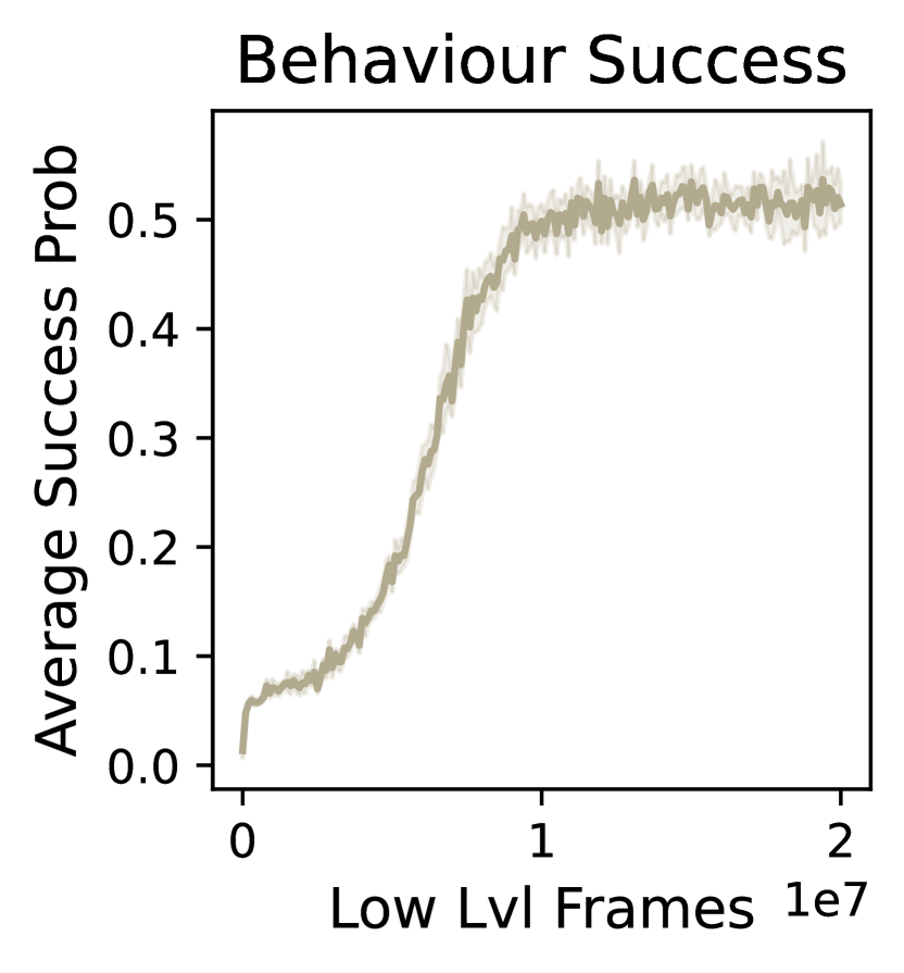
(a) Learning $\mathcal{B}$

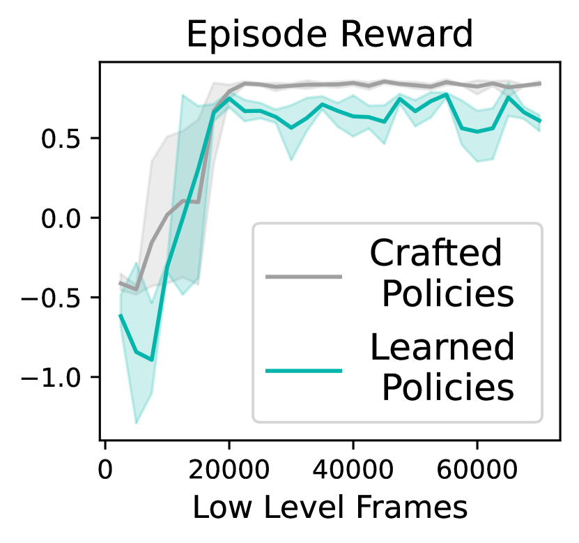
(b) Perf. with learned $\mathcal{B}$

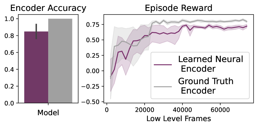
(c) Performance with learned object mapping

Figure 6: Performance using learned Ab-MDP components. All error bars denote 95 confidence interval of mean with exception of encoder accuracy which shows 1 standard deviation.

Up to this point we have assumed the existence of an object-centric mapping and competent behaviours (Sec. 2.1), which can be combined with our method for efficient exploration and world model learning. We now demonstrate how one might learn both components.

4.3.1 Learning low level policies

We observe low level policies can be learned with RL if an object-centric map exists. Specifically, we reward the agent for achieving an abstract transition successfully: from $X_{t}$, if executing behaviour $b=(\alpha^{(i)},\xi^{\prime})$ until an abstract transition results in $X_{t+1}$ containing item $(\alpha^{(i)},\xi^{\prime})$, the associated policy $\pi_{b}$ gets a reward of +1 (else -1). We train low level policies to replace all behaviours in the MiniHack single task environments, and observe the success probability can be stably optimized with PPO (Fig.6(a); note it does not reach 1 as it is averaged over all attempted behaviours, some are for impossible transitions). Solving Ab-MDP with learned behaviours perform similarly (Fig.6(b)). The reported 2D Crafting results (Section 4.1) already use learned behaviours. Details in Appendix F.2.

4.3.2 Learning object-centric map

If we wish to also learn the object-centric mapping, we can do so using supervised learning. We generate a dataset of 100k transitions using a random policy in MiniHack’s Freeze-Horn environment, and use the hand-crafted mapping to provide ground truth abstract state labels. We train a neural net to produce the abstract state $X$ from $S$. We compare planning performance using the learned object-centric mapping in Figure 6(c) and observe it reaches similar performance as the ground truth mapping, even though the encoder is not perfect in predicting the abstract states. We discuss alternative way of getting this mapping in Section 6.

4.4 Ablations

We ablate major design choices below, with additional ablations in Appendix F.3.

4.4.1 Generative vs. Discriminative Models

Figure 7: Planning performance with discriminative vs. generative models

A common way of learning a forward model is to model the next state generative-ly, i.e. $\hat{X}_{t+1}\sim f(X_{t},b_{t})$, with support over the entire state space $\mathcal{X}$. In MEAD, we opted to constrain the possible future to either be the same as the current time-step, or one where there is a single item change (Fig. 2). This has the disadvantage of being less flexible, but the advantage of being easier to model. To isolate only the effect of discriminative modelling, we design an experiment where we fit models to the same expert dataset, with the only difference being the model type (fit to either predict success probability in the discriminative case, or to predict the distribution over next item-attribute sets), while keeping all other variables constant. Indeed, given the same (expert) data budget, a discriminative model learns a better model for Ab-MDP planning in the lower data regime (Figure 7, experimental details in Appendix F.3.1).

4.4.2 Count-based exploration

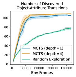
Figure 8: Effect of count-based exploration in the Freeze-Wand environment. MCTS discovers more unique valid (item identity, item attribute, new attribute) transitions.

We observe using the count-based intrinsic reward (Equation 4) with MCTS was important for exploration. Figure 8 (right) shows count-based exploration discovering many more valid object attribute transitions compared to a randomly exploring agent. Correspondingly, this leads to a model $f_{\theta}$ that is better at achieving goals (Figure 8, left).

4.4.3 Parametric vs. Non-Parametric Models

Instead of fitting a discriminative model to success probability, we can directly use the empirical count-based estimate from a dataset (a non parametric model). This is done to learn the model in Zhang et al., (2018). We compare this choice in Appendix F.1.3 and show our parametric model has better sample efficiency, demonstrating the generalization benefits of our parametric forward model.

5 Related Work

Hierarchical RL

Our Ab-MDP is a hierarchical state and temporal abstraction formalism and can be interpreted as Options (Appendix B.1). Within the Options Framework (Sutton et al.,, 1999; Precup,, 2000), Option discovery remains an open and important question. Existing methods typically do option discovery in a “bottom-up” fashion by learning structures from their training environments (Bacon et al.,, 2016; Machado et al.,, 2017; Ramesh et al.,, 2019; Machado et al.,, 2021). In contrast, our Ab-MDP uses “top-down” prior knowledge in the form of object-perception, and define options that perturb objects’ attributes.

Planning with abstract representations

Abstraction is a fundamental concept (Abel,, 2022) and we select a subset of most relevant works. The Ab-MDP can be viewed as a more structured MDP formulation in which learning and planning is simplified. This relates to OO-MDP (Diuk et al.,, 2008; Keramati et al.,, 2018), which describes state as a set of object and object states which interact through relations. Also related is MaxQ and AMDP (Dietterich,, 1998; Gopalan et al.,, 2017), which provides a decomposition of a base MDP into multi-level sub-MDP hierarchies to plan more efficiently. Transition dynamics can also be defined as symbolic domain specific language (Mao et al.,, 2023). Above works require pre-specifying additional interaction rules, functions, and object relations to simplify planning, whereas we only assume the ability to see objects and their attributes, and learn the forward model as a neural network. More distantly related is Veerapaneni et al., (2019) which focus more on learning good object-centric representations rather than effective usage of an abstract level. Nasiriany et al., (2019) tackles sub-policy learning and planning with abstraction, focusing on implicitly representing abstractions rather than using semantically meaningful ones. The DAC-MDP (Shrestha et al.,, 2020) clusters low level states into “core states” to solve by value iteration, with a focus on getting good policies in an offline RL setting rather than abstract world model learning.

Most similar is Zhang et al., (2018), which does model-based planning over abstract attributes. We differ in having a more expressive abstraction framework: modelling a flexible set of objects and shareable attributes, rather than a fixed, binary set of attributes only. We also use a parametric model to more efficiently learn and is able to transfer object information to new environments. We compare against their non-parametric approach and show better sample efficiency in Section 4.4.3.

RL in semantic spaces As language models have grown in interest and sophistication, there has been an increasing interest in semantic and linguistic abstractions in RL. Early works such as Andreas et al., (2017) looked at handcrafted abstract spaces such as we do here to show that creating abstractions allows for better learning and exploration. Other works such as Jiang et al., (2019); Chen et al., (2021) specifically use natural language as the abstract space. In others, the language space abstraction is used as a way of guiding exploration Tam et al., (2022); Guo et al., (2023).

Model-based RL

Our work is related to other work in Model-based Reinforcement Learning (Sutton,, 1990; Kaiser et al.,, 2019; Doya et al.,, 2002). In particular we compare to the Dreamer line of work (Hafner et al.,, 2019, 2023; Sekar et al.,, 2020; Mendonca et al.,, 2021; Hafner et al.,, 2022). These methods were developed for a pixels setting and employ a two step learning strategy: learning a generative forward model to predicts the next states $X^{\prime}$, then learning a policy in imagination. We compare directly to this in our experiments, where we show that our method (which employs a discriminative forward model) learns more quickly and transfers better in our setting.

Exploration in RL

Exploration is a well-studied problem in RL. For a more extensive literature review, Amin et al., (2021) gives a comprehensive picture. Most relevant to here are count-based methods such as Raileanu and Rocktäschel, (2020); Zhang et al., (2021). Our work takes inspiration from the hard exploration problems from  Henaff et al., (2022). There are also many disagreement-based methods including Sekar et al., (2020) and Mendonca et al., (2021); we compare directly to the former for our Dreamer benchmarks with pre-training.

6 Discussion

In this work we introduce the Ab-MDP, which uses human understandable object-attribute relations to build an abstract MDP. This enables us to learn a discriminitive model-based planning method (MEAD) which explores and learns this semantic world model without extrinsic rewards.

Limitations The major limitation of the work is that the construction of Ab-MDP requires the existence of an object-centric mapping. While we show how these components can be learned in Section 4.3, learning the object mapping still requires a labelled dataset. Promisingly, the field as a whole is moving in a direction where abstractions are becoming more easily obtainable. For instance, object-centric abstract maps can be acquired using segmentation models (Kirillov et al.,, 2023) and visual language models (Alayrac et al.,, 2022). Similarly, the short-horizon (low level) manipulation policies can be acquired more efficiently through imitation learning. In the robotics setting it’s even been found that using off-the-shelf models for these perception and skill policies is possible (Liu et al.,, 2024). Nevertheless, a method to automatically discover object-centric representations remains an open question.

7 Acknowledgements

This work is supported by ONR MURI #N00014-22-1-2773 and ONR #N00014-21-1-2758. AGC is supported by the Natural Sciences and Engineering Research Council of Canada (NSERC), PGSD3-559278-2021. Cette recherche a été financée par le Conseil de recherches en sciences naturelles et en génie du Canada (CRSNG), PGSD3-559278-2021. We are grateful for insightful discussions with Rajesh Ranganath. We thank Ben Evans, Siddhant Haldar, Ulyana Piterbarg, Dongyan Lin, and Mandana Samiei for their helpful feedback on earlier drafts of this paper.

Appendix

Appendix A Broader Impact

Our contributions are fundamental reinforcement learning algorithms, and we hope our work will contribute to the goal of developing generally intelligent systems. However, we do not focus on applications in this work, and substantial additional work will be required to apply our methods to real-world settings.

Regarding compute resources, we use an internal clusters with Nvidia A100 and H100 GPUs. All experiments use at most one GPU and are run for no more than two days. Running baselines along with randomization of seeds requires multiple GPUs at once.

Appendix B Problem Setting Details

B.1 Abstracted MDP

Here we re-iterate our framework and discuss it in greater details. We first define a low level (reward-free) Markov Decision Process (MDP, Puterman, (1994)) as the tuple $\langle\mathcal{S},\mathcal{A},P\rangle$, with (low level) state space $\mathcal{S}$, primitive action space $\mathcal{A}$, and transition probability function $P:\mathcal{S}\times\mathcal{A}\times\mathcal{S}\rightarrow[0,1]$. Suppose the agent interacts with the environments at discrete time-steps $u=0,1,2,...$, then $P(s_{u+1}|s_{u},a_{u})$ describes the probability of transitioning to state $s_{u+1}\in\mathcal{S}$ after one time-step when choosing action $a_{u}\in\mathcal{A}$ in the current low level state $s_{u}$.

To construct an Ab-MDP, we start with a surjective deterministic mapping M from low to abstract level: $\text{M}:\mathcal{S}\rightarrow\mathcal{X}$. That is, any low level state $S\in\mathcal{S}$ maps onto some abstract state $X\in\mathcal{X}$ (multiple $S$ can and do map to the same $X$).

Define behaviours $\mathcal{B}$. Each $b=(\alpha^{(i)},\xi^{\prime})\in\mathcal{B}$ describes a single item id $\alpha^{(i)}$ and a desired new attribute, along with an associated low level policy $\pi_{b}:\mathcal{S}\rightarrow\mathcal{A}$ which tries to set the specified item to have the new attribute. A behaviour can be competent or incompetent. Executing competent behaviours lead to the specified item-attribute changes with high probability.

A behaviour may be incompetent because (i) the proposed attribute change is impossible within the rules of the world (e.g. item is not a craft-able object) (ii) the attribute change is not possible from the current state (e.g. do not have the correct raw ingredients in inventory), or (iii) the behaviour is not sufficiently trained to perform the specified change.

We build a simple abstraction that allow us to learn purely at the abstract level while still being able to influence actions at the low level. Notice the surjective map M give us state abstraction. We build temporal abstraction by defining abstract state transitions as happening at a slower time-scale than the low level time-step $u$.

Definition B.1.

An abstract state transition has occurred at (low level) time-step $u$ if: (i) the abstract state has changed, $\mathcal{M}(s_{u})\neq\mathcal{M}(s_{u-1})$; or (ii) the abstract state has not changed in the past $k$ steps, $\mathcal{M}(s_{u})=\mathcal{M}(s_{u-1})=...=\mathcal{M}(s_{u-k})$.

Definition B.2.

An (max-k) Ab-MDP is defined as the tuple $\langle\mathcal{X},\mathcal{B},\textbf{T}_{k}\rangle$, with abstract states $\mathcal{X}$, abstract behaviours $\mathcal{B}$, and transition probability function $\textbf{T}_{k}:\mathcal{X}\times\mathcal{B}\times\mathcal{X}\rightarrow[0,1]$. $\textbf{T}_{k}(X^{\prime}|X,b)$ describes the probability of being in abstract state $X^{\prime}$ when starting from $X$ and executing behaviour $b$ until an abstract state transition occurs (Definition B.1).

In the main text, we write Ab-MDP and denote the transition function as T for brevity (instead of writing max-k Ab-MDP and transition function $\textbf{T}_{k}$). $k=8$ was chosen for baseline methods as it worked slightly better. MEAD works just as well with $k=8$ and $k=16$.

B.1.1 Interpretation as Options

It is natural to interpret our hierarchical framework within the Options framework (Sutton et al.,, 1999). An option consists of a policy $\pi:\Omega\times\mathcal{A}\rightarrow[0,1]$, a termination function $\beta:\Omega\rightarrow[0,1]$, and an initiation set of states $\mathcal{I}\subseteq\mathcal{S}$. $\Omega$ is used to denote the set of all possible historical states.

Our set of behaviour $b\in\mathcal{B}$ is a set of options. Each behaviour specifies a behaviour policy $\pi_{b}$, which deterministically terminate when an abstract state transition occurs (Definition B.1), and they can be initiated from all states ($\mathcal{I}=\mathcal{S}$).

The point of the Options Framework and temporal abstraction generally is to break up a monolithic problem into re-usable sub-problems. How one breaks up a problem is an open question. Some popular previous approaches include finding bottleneck states and using the successor representation to discover well-connected states. We can view our approach as another way of breaking up the problem when prior knowledge in the form of objects is available: we break up the problem at the level of single item-attribute changes (with options defined as policies that can change a single item’s attribute).

B.1.2 A note on semi-MDP

The decision process that selects amongst options is a semi-MDP (Theorem 1, (Sutton et al.,, 1999)). The general way to model semi-MDP dynamic requires considering the amount of low level timesteps that passes between each abstract level decision as a random variable (Sutton et al.,, 1999; Barto and Mahadevan,, 2003). Instead, we chose to simply treat the abstracted level as having a fixed time interval in between steps. This is chosen for simplicity as our focus is with learning efficiency on the abstract level, and this formulation allow us to directly apply efficient algorithms developed to solve MDPs. We also see empirically that given our $\mathcal{M}$ and $\mathcal{B}$ this choice does not lead to a less optimal policy compared to algorithms that directly solve the low level MDP.

B.1.3 Multi-Item Behaviours

In the Ab-MDP, we consider abstract states as an (ordered) set of items $X=\{x^{(1)},x^{(2)},...\}$, where each item consist of an identity and attribute $x^{(i)}=(\alpha^{(i)},\xi^{(i)})$. A behaviour is a description of which item(s) to change (Section 2.1). For instance, the single-item behaviour $b=\{(\alpha^{(i)},\xi^{\prime})\}$ specifies a change of the $i$-th item to a new attribute $\xi^{\prime}$. We can similarly specify multi-item behaviours, such as a two-item behaviour $b=\{(\alpha^{(i)},\xi^{\prime}),(\alpha^{(j)},\xi^{\prime\prime})\}$. This behaviour is competent if after an abstract state change, the $i$-th item takes on attribute $\xi^{\prime}$ and the $j$-th item takes on attribute $\xi^{\prime\prime}$ with high probability.

For $N$ objects, $m$ attributes, and $I$ items changes to consider in behaviours,

$$\text{Number of behaviours}=\binom{N}{I}\times m^{I}\,.$$ (6)

For instance, for single item change behaviours ($I=1$), there are $\binom{N}{1}\times m^{1}=N\times m$ behaviours. For two-item change behaviours ($I=2$), there are $\binom{N}{2}\times m^{2}$ behaviours, and so on. In the extreme, one can choose to model a all possible item attribute changes ($I=N$), which results in $m^{N}$ behaviours that is exponential in the number of items considered.

B.2 Analysis of Assumptions

B.2.1 The generality of Ab-MDP

One may worry that the abstraction specified by Ab-MDP is overly specific to a particular problem and an appropriate abstraction would not exist for a different problem. To this end, we make the following observation that any sparse reward RL task can be described by a Ab-MDP with a single item,

Remark B.3.

For any MDP with a reward function $R:\mathcal{S}\rightarrow\mathbb{R}$, where,

$$R(S)=1\text{ if }S\in\mathcal{G}\text{ and }0\text{ otherwise}\,,$$

for $S\in\mathcal{G}$ terminal goal state(s), we can describe this as an Ab-MDP with a single item $\alpha$ and binary attributes $\{\xi_{1},\xi_{2}\}$. The abstract map $\text{M}:\mathcal{S}\rightarrow\mathcal{X}$ can be constructed in the following way,

$$\text{M}(S)=\begin{cases}\{(\alpha,\xi_{2})\}\quad&\text{if }S\in\mathcal{G}\,,\\ \{(\alpha,\xi_{1})\}\quad&\text{otherwise}\,.\\ \end{cases}$$ (7)

The proxy problem of transition from $X=\{(\alpha,\xi_{1})\}$ to $X=\{(\alpha,\xi_{2})\}$ solves the sparse reward task in the base MDP and a competent behaviour for this transition is a good policy is the base task.

The point of this is merely to say that Ab-MDP does not restrict the RL problem in a particular way. Of course, such a construction of an Ab-MDP is not interesting and learning a competent behaviour for this Ab-MDP is no easier than learning a behaviour that maximizes the reward function in the base MDP.

The point of Ab-MDP, however, is that a task can be broken-up in a more interesting way, e.g. in our case through a richer set of items and attributes. We demonstrate in this work that an object-centric item-attribute set encoding result in a set of intuitively base behaviours and a world model that is interesting.

B.2.2 Discriminative modelling with single item change

In our forward model, we made the assumption to only model single item’s attribute change (Section 3.1 and Equation 3), and that if the attribute does not change then the abstract state $X_{t+1}$ stays the same as $X_{t}$. We analyze this assumption more deeply in this section.

Robustness through re-planning

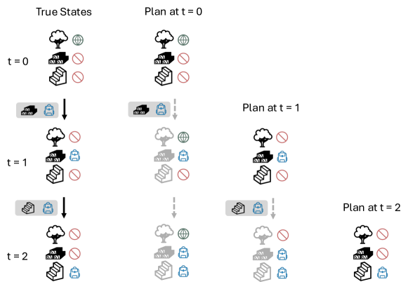
Figure 9: An illustrative example following the logic of the 2D Crafting game. The objective of the game is to get planks by chopping trees (which changes the plank’s attribute from absent to in inventory, and the tree’s attribute to from in world to absent as the resource is depleted), then craft wooden stairs using the plank (which depletes the plank resources to absent and creates wooden stairs in inventory). Comparing the true state trajectory with the imagined plan at t=0, we notice that the imagined future is incorrect: modelling only single item changes do not capture the fact that resources are depleted, but only new resources are created. Nevertheless, at t=1, the model observes the new abstract state and can therefore re-plan with the most up-to-date information which corrects for previously incorrect predictions. A case like this happens in practice within the 2D Crafting games.

We first note that in practice, it is often the case that multiple item’s attribute changes. For instance, in the 2D Crafting environments, crafting an item often consumes the raw ingredient used to craft it. Thus, a plan that considers multiple items being crafted (attribute change from absent to in inventory) will inaccurately predict that the raw ingredient stays in the inventory (attribute of raw ingredient stays the same, staying as in inventory) rather than changing to absent. We illustrate the plan generate at each abstract step in Figure 9, and show that despite this being the case, the plan still generates an optimal action sequence; and that at each time-step, re-planning with the newly obserbved abstract state updates the incorrect abstract prediction to be more accurate.

An adversarial failure case

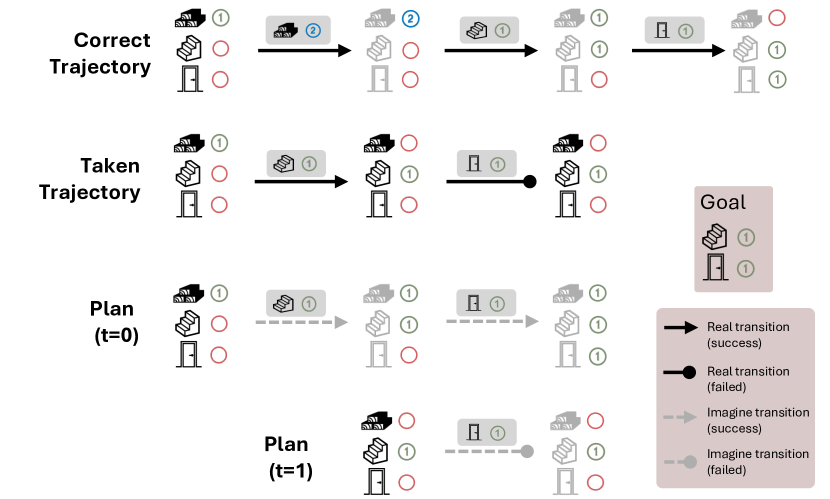
(a) Planning with single item-attribute changes fails in this adversarial task.

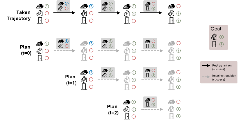
(b) Planning with double item-attribute changes models attribute dynamics perfectly.

Figure 10: Single and double item-attribute change planning

Here we artificially design an adversarial setting which is not encountered in our evaluation environments, but would in theory result in sub-optimal plans. With reference to Figure 10(a), we construct an environment whose goal is to construct both a wooden stair and a wooden door. Both require a single unit of wooden plank to craft. The attribute here is the quantity of the item in the inventory. Suppose further that once we start crafting, we can no longer collect additional wooden planks.

The correct sequence of behaviour would be to first collect another unit of wood, before crafting a wooden stairs and a wooden door. Planning with a discriminative single item change model would result in a sub-optimal plan, as it fails to consider that crafting a wooden stair result in the wooden plank being consumed, and therefore cannot subsequently craft the wooden door (Fig.10(a), plan at t=0).

Note that this failure case is a limitation of doing discriminative modelling with single item changes (Section 3.1), not the Ab-MDP framework. Doing generative modelling (considering all possible $X_{t+1}\in\mathcal{X}$ given $X_{t},b_{t}$) would be able to learn the correct relationship—at the cost of data inefficiency (Section 4.4.1). Nevertheless, we discuss how to fix it below with discriminative modelling.

Discriminative modelling of multi-object changes

One simple way of generating plans with multi-item dependencies over time is to consider multi-item behaviours (Section B.1.3). With reference to Figure 10(b), we notice that simply modelling two item changes can perfectly capture the dynamics within this task and generate the optimal plan. This comes at a cost of a greater number of behaviours to consider at each step of planning (E.g. for $N=3$ items, $m=3$ attributes, there are 9 behaviours to consider for single-item changes, and $27$ behaviours to consider for two-items changes).

Generally speaking, with a small change in the representation of the problem, we can plan to generate the optimal sequence of abstract behaviours. This can also happen through changing the abstract mapping—e.g. by modelling items along with the resources needed to create them. Overall, we view this as a problem of constructing the right abstraction for the problem which, although important, is not the main focus of this work and nor a fundamental issue with our modelling choice.

Appendix C MEAD: Extended Methods

Here we provide more details about our methods

C.1 Model Fitting

Given a dataset of (abstract) trajectories collected via the exploration strategy outlined in Section 3.2, $\mathcal{D}=\{(X_{1},b_{1},X_{2},b_{2},...)_{i}\}_{i=1,...,n}$, we can estimate the empirical success probability $q$ of all observed item-attribute pairs by counting their occurrences:

$$q(X,b)\approx\rho(X,b)=\frac{\text{Number of $(X_{t},b_{t},X_{t+1})$ transitions where }(\alpha^{(i)},\xi^{\prime})\in X_{t+1}+\epsilon}{\text{Number of $(X_{t},b_{t})$}+2\epsilon}\,,$$ (8)

where $\epsilon$ is a small smoothing constant (usually 1e-3). This can be efficiently implemented as a hash map, via hashing $(X_{t},b_{t})$ as keys, and the number of successful and total transitions (starting from $(X_{t},b_{t})$) as values.

To train our discriminative model $f_{\theta}:\mathcal{X}\times\mathcal{B}\rightarrow[0,1]$, we minimize binary cross entropy loss with $\rho$ as the target,

$$\theta^{*}=\arg\min_{\theta}\mathbb{E}\left[\rho(X,b)\cdot\log\left(f_{\theta}(X,b)\right)+\left(1-\rho(X,b)\right)\cdot\log\left(1-f_{\theta}(x,b)\right)\right]\,,$$ (9)

where the expectation is estimated by uniformly sampling unique $(X,b)$ pairs from dataset.

Appendix C.2 contains architectural details for $f_{\theta}$. All in all, we found that our sampling method and loss function lead to a stable, simple-to-optimize objective. Moreover, it is possible to directly use $\rho$ to do planning, as is done in Zhang et al., (2018). However, we show in Section F.1.3 that it is more efficient to use our parametric modelling approach as it generalizes better to new objects.

Algorithm 1 Example Data Collection and Training loop for MEAD

0:  Model $f_{\theta}$

  repeat

     Collect $n$ frames of data in environment using model $f_{\theta}$ to plan to explore

     Add data to dataset $\mathcal{D}$

     Reset model weights $\theta$

     while accuracy requirement not met do

        if local minima then

           Reset model weights $\theta$

        end if

        Sample from $\mathcal{D}$ and minimize Equation 9, for $m$ optimizer steps

     end while

  until time runs out

We provide the pseudocode for training MEAD in Algorithm 1. The accuracy requirement is a running average binary classification accuracy (typically set to 0.95). The local minima is evaluated by checking if the difference is accuracy is close to zero (taken as a exponentially smoothed average to be insensitive to stochasticity). We find in Figure 26 that the most important setting is to run enough gradient updates between data collection steps—the precise setting of checking for accuracy and local minima does not matter as much.

C.2 Model Architecture

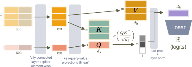
Figure 11: Model Architecture

We use a small key-query attention architecture that takes in sets of vectors to produce a binary prediction, see Figure 11.

C.3 Exploration

We use a reward function that encourages indefinitely exploring all states and behaviours,

$$r_{\text{intr}}(X,b)=\sqrt{\frac{T}{\text{N}(X,b)+\epsilon T}}\,,$$ (10)

where $\text{N}(X,b)$ is a count of the number of times $(X,b)$ is visited, $T$ is the total number of abstract time-steps, and $\epsilon=0.001$ is a smoothing constant.

Intuitively, a state with many visits (large $\text{N}(X,b)$) will have lower reward, while $T$ prevents the intrinsic reward from shrinking to zero (so the agent explores indefinitely). Indeed, in the bandits setting, this reward function is maximized when all states are visited uniformly (Zhang et al.,, 2018). We emphasize that all of our model training is done with this intrinsic reward, with no task-specific information injected at training time.

We use MCTS to find high (intrinsic) reward states. MCTS iteratively expands a search tree and balances between exploring less-visited states (using an upper confidence tree) and exploiting rewarding states. In our case, MCTS generates child nodes of abstract state $X$ by proposing behaviours $b$ and checking if $f_{\theta}(X,b)>0.5$ (Figure 3(a)). We also introduce a small degree of randomness so all behaviours have a small chance of being selected.

We modify the MCTS algorithm to return the the maximum $r_{\text{intr}}(X,b)$ encountered along each path during the back-propagation stage and set a fix expansion depth without a simulation stage from the leaf node. This is done to prevent loops and encourage the agent to go toward frontier states with the least amount of visitations.

Appendix D Environments

D.1 2D Crafting

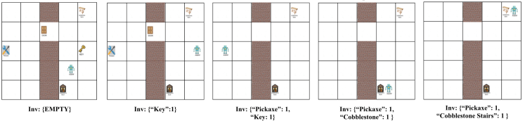
Figure 12: Example episode in an example 2D Crafting environment, figure taken from Chen et al., (2020). To solve this task, the agent needs to pickup the pickaxe, mine the cobblestone stash to get cobblestone, then use the acquired cobblestone to craft cobblestone stairs. The items must be acquired in that order as each step requires having the item from the previous step (with an additional obstacle of being able to cross the door only if it has a key).

We adopt three crafting environments proposed in Chen et al., (2020), which contain Minecraft-like crafting logic. The agent needs to traverse a grid world, collect resources, and build increasingly more complex items by collecting and crafting ingredients (e.g. getting an axe, chopping tree to get wood, before being able to make wooden planks and furniture that depend on planks). Primitive actions consist of movement in the four cardinal directions (N,E,S,W), toggle (of a switch to open doors), grab (e.g. pickaxe), mine (e.g. ores), craft (at crafting bench of specific items). The low level observation space consist of a dictionary containing: (i) an (5, 5, 300) matrix describing a $5\times 5$ world with each state being described by an 300-dim word embedding, (ii) an 300-dim inventory embedding describing things in the inventory, and (iii) a 300-dim goal embedding describing in words the task to complete. We describe each environment’s crafting sequences required to finish each task in Table 1.

Environment Name	Crafting Task Description
2 Steps	Pickup pickaxe, mine gold ore
3 Steps	Pickup pickaxe, mine diamond ore, craft diamond boots
4 Steps	Pickup axe, chop tree to get wood, craft wooden plank from wood,
	then craft either wooden stairs or wooden door from plank

Table 1: 2D Crafting environments.

Abstraction States

We build a simple abstraction to map from the low level observation to an abstract representation. We take as items all objects in the world, in the inventory, and potentially craft-able objects. We assign each item one of the the attributes in Table 2.

We take each item identity as its 300-dim word embedding provided from the environment, and each attribute as a one-hot embedding, repeated to also be 300-dim. Each item in the item set is described as a 600-dim vector.

Attribute	Description
IN_WORLD	An item is in the world but not in the inventory.
IN_INVENTORY	An item is in the player’s inventory.
ABSENT	An item is neither in the inventory or in the world.

Table 2: 2D Crafting attributes.

D.2 MiniHack

We also use the MiniHack environment (Samvelyan et al.,, 2021), which is built on the Nethack Learning Environment (Küttler et al.,, 2020). We use five hard-exploration games from Henaff et al., (2022) requiring interaction with different types of objects. The base game has a multi-modal observation space involving image, text, inventory, etc. Solving the game from the base observation is extremely difficult since each environment has multiple variants of an object (e.g. Freeze-Wand has 27 different types of wands), and randomly generated object locations. Indeed, Henaff et al., (2022) found that performant RL methods such as IMPALA (Espeholt et al.,, 2018; Küttler et al.,, 2019) and all tested global exploration methods (ICM (Pathak et al.,, 2017) and RND (Burda et al.,, 2019)) fail to solve these environments.

The base environment contains an dictionary observation space, containing a $21\times 79$ grid of glyphs (integer denoting one of 5976 nethack glyph types), an 27-dimensional vector denoting agent’s stats, a 256 dim vector for message, and another vector denoting agent’s inventory. The environments are:

• "MiniHack-Levitate-Boots-Restricted-v0"

• "MiniHack-Levitate-Potion-Restricted-v0"

• "MiniHack-Freeze-Horn-Restricted-v0"

• "MiniHack-Freeze-Wand-Restricted-v0"

• "MiniHack-Freeze-Random-Restricted-v0"

Generically, the Nethack Learning Environment contains over 100 actions; whereas the “restricted” set of games reduce this space. The possible primitive actions include the 8 cardinal actions (N, E, S, W, NE, SE, SW, NW), PICKUP, ZAP, WEAR, APPLY, QUAFF, PUTON, FIRE, READ, and RUSH. It may be even less dependeing on the specific environment.

Abstract States

We hand-construct a map that maps from the multi-modal observations to a set of (object identities, object attribute) vectors. We do this by taking the glyph and inventory observation modalities and filtering out all glyphs containing blank spaces, floor, and walls. To get the object attributes, We take the remaining glyphs and mark them as being “in world” if they are in glyph, and “in inventory” if they were from the inventory modality. Then, if the agent object was beside an object and took a primitive action to move towards it, we mark the object as “standing on”. If we observe a levitating message (e.g. “up, up and away” from the message modality, we set the agent object to have “levitate” attribute. Alternatively, if the low level episode terminates along with the last observation being either a levitate message or a “freeze spell” message (e.g. “the frozen bolt bounces”), then we set the corresponding levitate or freeze object to have “used” status. Finally, if an object disappears from the low level observation that is not being stood on, we set it to have “removed” attribute. We summarize this in Table 3.

Attribute Name	Meaning	How to Infer
in world	The object is in the world	Object is in the glyph observation
standing on	Object in world, and the	Object was in the glyph observation
	player is standing on it	and message says “you see here…”
in inventory	Object in inventory	Object in the inventory observation
levitating	Agent is levitating	Message says a levitate message
used	An object is used	A freeze or levitate message appears,
		and episode terminates
removed	Object disappears from world	The object is not longer present

Table 3: Object Attributes and how to infer them.

As for object identities, they are simply the glyph number given to them in MiniHack (e.g. 329 for the player agent).

Embeddings

We then embed the object identities and attributes before providing them to the agents. For object identities, we take each object’s glyph number, and map it to the NetHack text description for that glyph (which we can extract from the screen_descriptions modality in the low level observation). For each glyph’s text description (which is a short sentence), we pre-process the sentence to remove stop words, then take each word’s GloVe (Pennington et al.,, 2014) embedding and averaging over the sentence. We use the 300-dimensional Wikipedia 2014 + Gigaword 5 GloVe word vector embeddings from https://nlp.stanford.edu/projects/glove/ (6B tokens, 400k vocab, uncased). The 300-dim vectors were chosen as we found them to have naturally good separation between object types in preliminary analysis.

We embed the object attributes as 300-dimensional one-hot vectors (i.e. one-hot between six categories and repeated to fill 300 dimension). This is done to make sure the input space is equally represented by the identity and attribute embeddings.

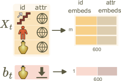
Figure 13: Embedding

D.2.1 Sandbox Environment

Figure 14: Sandbox Minihack environment

We design a sandbox environment where the agent can observe and interact with all items it may encounter in one of the five evaluation environments. In the sandbox, each of these objects has an 0.5 chance (independently) of spawning at a random location: levitate boots, levitate rings, levitate potions, freeze horn, freeze wands. Further there is a 0.5 change that a second of the same object type will spawn. The agent can interact with any of the objects for up to 250 low level frames, or the episode terminates once the agent sets any of the object’s attribute to “used”. Figure 14 shows an instantiation of an episode.

D.2.2 Low Level Policy Errors

The learned and hand-defined low level policies are not perfect. We see that depending on the initial abstract state, the low level policy succeeds on average around 90% of the time, but can be as low as 10% for particular states (Figure 15).

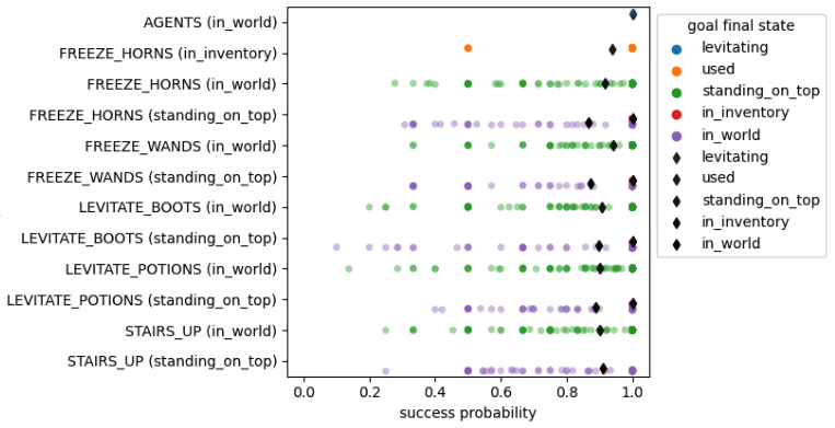
Figure 15: Low-Level policy success rates for an environment

Some common failure cases for these low-level policies are:

1. To use an item in the inventory, the policy needs to select which item to use (e.g. to drink a potion the policy needs to first do primitive action "quaff", then primitive action that selects the inventory object to drink, etc.). When there are multiple objects in the inventory it just picks a random object, meaning it might not pick the object specified by the behaviour

2. The “go stand on” policy is coded to move in a straight line towards an object. Since we measure a policy "success" whenever the abstract state changes, if the agent walks over another object en route, the Ab-MDP will register an abstract state change and deem the transition unsuccessful

3. To successfully cast a freeze spell, the NetHack game needs to return a message saying the spell has bounced off a wall. To our knowledge, this is stochastic—we got as far as figuring out that the spell needs to travel sufficient distance to bounce, but even so we were unable to produce a low level policy that results in spell bounce 100% of the time. This succeeds 8̃0% of the time

Appendix E Baseline Methods

For baselines, we use an environment wrapper which abstracts away the low level observations into only the abstract level observations and behaviours (as described in Section 2.1). We similarly equip the baseline policies with transformer-based encoders, with input masking in places where the input sequence is longer than the number of objects in the set as well as positional embedding, which we found in preliminary experiments helped with training. For action spaces, the agent generates a discrete integer action which maps onto an object index in the observation set as well as the object attribute to change to.

Specifically, we use Dreamer-v3 as a performant model-based baseline (Hafner et al.,, 2023), and PPO as a model free baseline (Schulman et al.,, 2017; Petrenko et al.,, 2020). For exploration-reward transfer experiments, we use a disagreement-based model for Dreamer intrinsic reward (Sekar et al.,, 2020), as well as using the same count-based reward to train all models.

Appendix F Extended Results

F.1 Extended Main Results

All runs, extended and main, are run with a minimum of 3 independent seeds.

To get the performance of the various algorithms in the low level MDP as we plotted them in Figure 4(b), we extracted them from Figure 13 in Henaff et al., (2022), using the WebPlotDigitizer app (https://apps.automeris.io/wpd/).

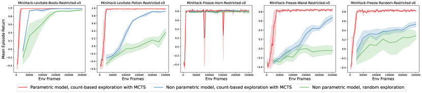
Figure 17: Training from scratch with different model types

F.1.1 PPO All Runs

We plot all PPO runs with different pre-training settings in Figure 18. Pre-training resulted in only negative transfer as compared to no pre-training.

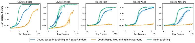
Figure 18: PPO all runs.

F.1.2 Dreamer

We show extended transfer results for Dreamer. We see in Figures 19 and 20 that when trained for much longer, Dreamer with both disagreement-based and count-based pre-training does start to get more rewards. However, we also observe the reward curves with pre-training is much worse than the reward curves without pre-training (black dotted lines), indicating negative transfer across environment and object types for these methods.

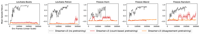
Figure 19: Longer Dreamer pretraining runs in the sandbox environment to show eval reward does increase with more samples, albeit pretraining seems to result in negative transfer.

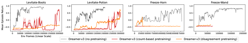
Figure 20: Longer Dreamer pretraining runs in the Freeze Random environment to show eval reward does increase with more samples, ableit pretraining seems to result in negative transfer.

F.1.3 Non-Parametric Model

We plot comprehensively the non-parametric model results in Figure 21.

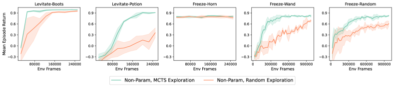
(a) Mean episode return

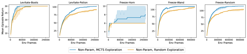
(b) Number of unique (Object, Attribute, New Attribute) transitions discovered

Figure 21: Non-parametric agent. Notice the difference in X-axis scale for Freeze-Wand and Freeze-Random environments.

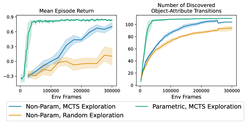
(a) Training from scratch with parametric (ours) and non-parametric model types in the Freeze-Wand environment. (Left) Episode return. (Right) Number of unique valid (item identity, item attribute, new attribute) transitions discovered.

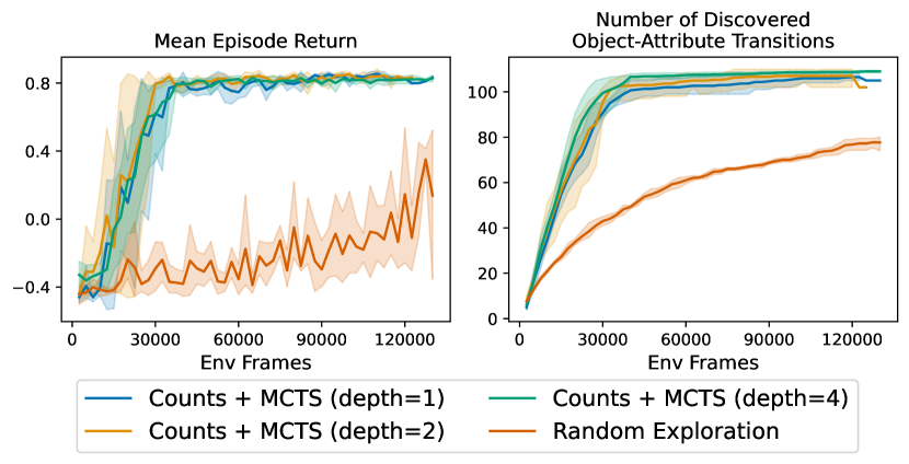
(b) Effect of count-based intrinsic reward and MCTS in the Freeze-Wand environment. (Left) Episode return. (Right) Number of unique valid (item identity, item attribute, new attribute) transitions discovered by the agent.

Figure 22: Model ablations

F.2 Low Level Learning

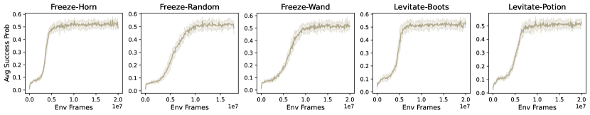
(a) Low level model free RL to optimize behaviour success probabilities

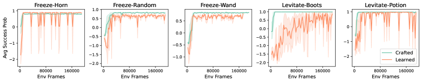
(b) MEAD performance in Ab-MDP with learned vs. crafted behaviours

Figure 23: Learning low level behaviours within MiniHack

We can reinforcement learn low level behaviours. From some $X_{t}$, we propose behaviour $b=(\alpha^{(i)},\xi^{\prime})$ and execute $\pi_{b}$ until an abstract transition. If the resulting $X_{t+1}$ contains item $(\alpha^{(i)},\xi^{\prime})$, we reward $\pi_{b}$ with a reward of +1 (else -1).

While this can be implemented in many ways, in practice we use a goal conditioned RL set-up, where a single model free policy network takes in both the low level state and the behaviour embedding to produce a primitive action: $\pi:\mathcal{S}\times\mathcal{B}\rightarrow\mathcal{A}$. The low level state is the environment’s raw observations while the behaviour embedding is the same as the one given to the abstract level model. This is implemented as a wrapper over the original environment which provides the policy with a +1 reward if $(\alpha^{(i)},\xi^{\prime})\in X_{t+1}$, and -1 otherwise. We use APPO as the policy optimization algorithm (Petrenko et al.,, 2020). The point of this is merely to show that we can learn the set of behaviours neurally and building an Ab-MDP with them still works.

The full MiniHack low level policy learning result is shown in Figure 23(a). The performance of MEAD in an Ab-MDP with learned behaviours is shown in Figure 23(b). Note that the reported 2D Crafting results in main text Section 4.1 already use neurally learned behaviours.

F.3 Extended Ablation Results

F.3.1 Generative and Discriminative Modelling

We design an experiment where we isolate the difference made by the generative vs. discriminative modelling, which we can view as a constraint over the support of the predicted distribution for $X_{t+1}$.

We collect a dataset using a hand-crafted expert policy in MiniHack’s Freeze-Horn environment, with a degree of action noise added to increase coverage. This is done to remove the exploration problem: the model only needs to learn to fit the trajectories well and it should contain within its world model the correct transitions required to solve the task. We fit two models:

• A discriminative model, which learns to predict success probability (Equation 1) as described by the main text.

• A generative model, which learns to predict the distribution over $\mathcal{X}$.

The two models use the same architecture to encode the previous abstract state and behaviours. It differs only in its output head: the discriminative model outputs a binary prediction, while the generative model outputs a categorical prediction for each item. We observe in Figure 24 that both model classes optimize the loss.

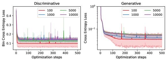
Figure 24: Loss curves for training generative and discriminative mdoels on a fixed expert dataset. Colors denote different number of dataset transition size.

To do planning, we run Dijkstra, with the edge weight as the negative log of $\Pr(X^{\prime}|X,b,\theta)$ (where $\theta$ denotes the generative or discriminative model). There are two ways we can generate the neighbours for the generative model: either by proposing the modal next state, i.e. $X^{\prime}=\arg\max_{X^{\prime}}\Pr(X^{\prime}|X,b,\theta)$, or by expected behaviour change $X^{\prime}=\Delta(X,b)$. Using expected behaviour change does not work in planning (the model never proposes behaviour sequences that lead to solving the task), thus we report results by using the modal next state. The results are reported in main text Figure  7, noting the error bars denote standard error of mean.

F.3.2 Model fitting

We found that running sufficient number of model fitting steps in between data collection steps was important. Fully re-setting the weights before data fitting is also helpful.

F.3.3 Semantic Embeddings

F.3.4 GloVe Embedding

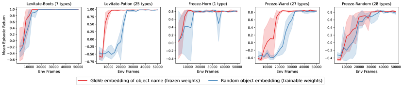
Figure 25: Training from scratch with frozen GloVe embeddings, or trainable randomly initialized weights.

We investigate the impact of having the object identity embeddings be semantically meaningful versus random one-hot embedding in MiniHack. By default, all experiments in the main text take as input object identity embedding using GloVe Pennington et al., (2014) embedding, which are kept frozen throughout training. We ablate this by initializing the object identity embedding matrix to be randomly initialized from a standard Gaussian, $\mathcal{N}(0,1)$, and allow them to be updated by gradients.

Figure 25 shows the results in all five games. We observe that having word embedding helps a bit in environment where there are many types of the same objects (i.e. Levitate-Potion and Freeze-Wand). This is unsurprising as the text embedding between objects would be rather similar (e.g. “wooden wand” and “metal wand” would have similar averaged embedding). Abeit they still performant overall. This hints at the abstraction being useful mainly due to its (object identity, object attribute) structure.

F.4 Model Updates

We show effects of number of model update steps during data collection in Figure 26,27,&28.

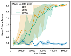
(a) Effect of model update steps between data collection steps.

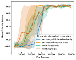
(b) Effect of model threshold logic prior to being allowed to collect more data

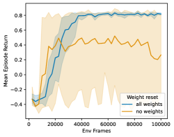
(c) Weight reset strategies before fitting on new data

Figure 26: Model training hyperparameters training in Freeze Wand environment.

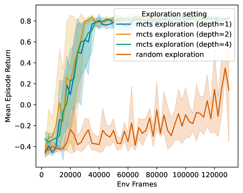
(a) MCTS hyperparameter effects, planning to find the max rewarding state using current parametric model.

(b) Using the empirical dataset probability for MCTS planning (i.e., a non-parametric estimate)

Figure 27: MCTS exploration hyperparameters in the Freeze Wand environment.

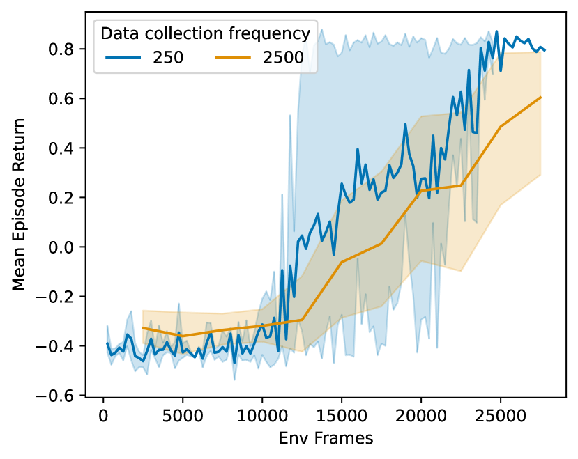
(a) Eval performance as function of data collection

(b) Wallclock time for different data collection frequencies

Figure 28: Data collection frequency in the Freeze Wand environment.

F.5 Model Embedding

We investigate the vector representation of different (object identity, object attribute) pairs in our model at the start of training and in the end. Results are shown in Figure 29. We observe vector cluster mainly along object attributes in the start of training (due to the orthogonal object embedding initialization). After training, vectors cluster by object attributes in an identity-dependent way. For instance, the STAIRS_UP object in Figure 29a are not clustered by attributes along the first two principle components in the Freeze Random environment, likely due to their usage being very different as compared to the other usable objects. We also observe separation by object-identities inside each of the object attribute clusters after training, but not before.

Again referring to Figure 29 (a), we notice that unseen objects (not seen in the Freeze Random environment—here it is the “levitate” objects) largely fall into clusters by attributes.

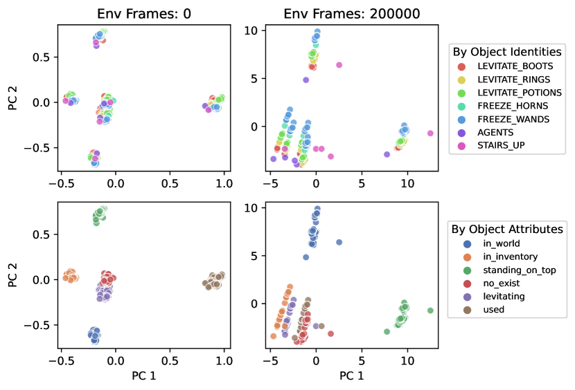
(a) Training in Freeze Random environment. Per dimension variance ratio explained at 0 frame: (0.24735658, 0.22067907); at 200k frames: (0.49951893, 0.35679522)

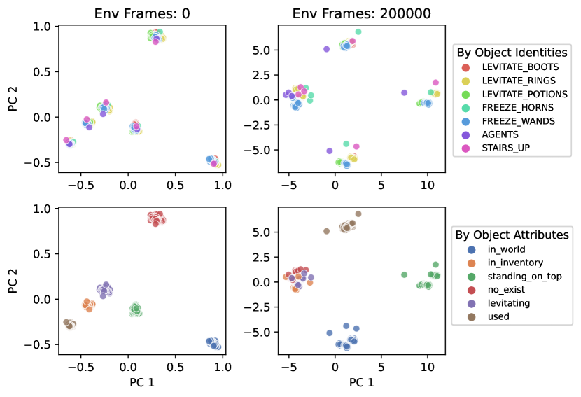
(b) Training in the Sandbox Playground environment. Per dimension variance ratio explained at 0 frame: (0.3139481, 0.23430094); at 200k frames: (0.5275301, 0.23016657)

Figure 29: Principle components analysis (PCA) of the (object identity, object attribute) vector representation in the model right before the key-query-value projection layer. PCA projects from 128 dimensions to 2 orthogonal dimensions of maximum variance. We show the representation at two points in training: 0 frames and 200k frames (columns). We label each (object identity, object attribute) vector by its identity (top row) and by its attribute (bottom row) separately.

F.6 Internal World Graphs

We can also show the model’s internal world model in a highly interpretable way: through running a graph search algorithm (e.g. breadth first search) along transitions the model predicts is high probability, and reconstructing the model’s internal graph.

We do this for two environments, showing only high probability transitions, and disallow visualization of loops in the graphs. The world model graph for Freeze-Random is in Figure 30. Note this is the same model which we illustrated in brief in main text Figure 3(b). The world model graph for a 200k frames checkpoint in the Levitate-then-Freeze environment is in Figure 31, which is much more complex even with only the high probability edges.

Figure 30: Extracted internal world model with a particular starting state in Freeze-Random by starting traversal from a given initial state. Only the most relevant objects are included for clarity and only transitions with success probability above 0.1 are included. Note that each node has 40-50 edges, although we only visualize the high probability ones.

Figure 31: Extracted internal world model by starting traversal from a given initial state. Only the most relevant objects are included for clarity. The plan required to solve the Levitate-then-Freeze task involves going from the top (root) state to the bottom left state.

Appendix G Training Details and Hyperparameters

G.0.1 Our model

We describe our default parameters in Table 4.

Hyperparameter		Value
Optimization	Optimizer	Adam
	Learning rate	1e-4
	Adam betas	(0.9, 0.999)
	Adam eps	1e-8
	Max batch size	2048
Data Collection	Additional frames before training	2500
	Weight reset before training	reset all weights
	Minimum optimizer steps before data collection	2500
MCTS Exploration	Random goal selection probability	0.2
	Num simulations	16
	Max search depth	4
	Probability for valid edge	0.5
Eval Planning	Dijkstra max iters	100
	Dijkstra low probability cut-off	0.1

Table 4: Default training parameters for our model

G.0.2 Dreamer-v3

We describe the default parameter used to run the Dreamer-v3 baseline. We use a PyTorch implementation of Dreamer: https://github.com/NM512/dreamerv3-torch, which has similar training curves as reported initially in Dreamer-v3. Unless otherwise mentioned, we use the “XL” world model setting with the highest amount of training iteration, which had the best reported sample efficiency in Hafner et al., (2023), and was confirmed by our preliminary experiments. We start with parameters as faithful to the reported ones in Hafner et al., (2023) as possible as it was found to work across a wide range of settings, then sweep over a subset of hyperparameters and report the best ones (which we use) in Table 5.

We perform parameter sweep over a subset and report the best ones (which we use) in Otherwise we keep the parameters as faithful to the reported ones in Hafner et al., (2023) as possible as it was found to work across a wide range of settings.

Hyperparameter		Value
Optimization	Optimizer	Adam
	Model lr	1e-4
	Actor lr	3e-5
	Critic lr	3e-5
	Batch size	32
	Batch length	64
	Train ratio	1024
	Replay capacity	$10^{6}$
Model Units	GRU recurrent units	4096
	Dense hidden units	1024
	MLP layers	5
Planning	Imagination horizon	15
Exploration (disagreement)	Ensemble size	10

Table 5: Dreamer parameters

G.0.3 PPO

We use the Sample-Factory implementation of PPO (Petrenko et al.,, 2020). We run a parameter sweep over a subset and report the best parameters which we use in Table 6.

Hyperparameter		Value
Data Collection	Number of workers	2
	Number of env per worker	10
	Rollout length	128
	Recurrence length	2
Optimization	Optimizer	Adam
	Model lr	1e-4
	Reward scale	1.0
	Batch size	4096
	Shuffle minibatches	False

Table 6: PPO Parameters

References

- Abel, (2022) Abel, D. (2022). A theory of abstraction in reinforcement learning. ArXiv, abs/2203.00397.
- Alayrac et al., (2022) Alayrac, J.-B., Donahue, J., Luc, P., Miech, A., Barr, I., Hasson, Y., Lenc, K., Mensch, A., Millican, K., Reynolds, M., Ring, R., Rutherford, E., Cabi, S., Han, T., Gong, Z., Samangooei, S., Monteiro, M., Menick, J., Borgeaud, S., Brock, A., Nematzadeh, A., Sharifzadeh, S., Binkowski, M., Barreira, R., Vinyals, O., Zisserman, A., and Simonyan, K. (2022). Flamingo: a visual language model for few-shot learning. ArXiv, abs/2204.14198.
- Amin et al., (2021) Amin, S., Gomrokchi, M., Satija, H., van Hoof, H., and Precup, D. (2021). A survey of exploration methods in reinforcement learning. ArXiv, abs/2109.00157.
- Andreas et al., (2017) Andreas, J., Klein, D., and Levine, S. (2017). Modular multitask reinforcement learning with policy sketches. In ICML, pages 166–175. JMLR. org.
- Bacon et al., (2016) Bacon, P.-L., Harb, J., and Precup, D. (2016). The option-critic architecture. ArXiv, abs/1609.05140.
- Barto and Mahadevan, (2003) Barto, A. G. and Mahadevan, S. (2003). Recent advances in hierarchical reinforcement learning. Discrete Event Dynamic Systems, 13:41–77.
- Burda et al., (2019) Burda, Y., Edwards, H., Storkey, A., and Klimov, O. (2019). Exploration by random network distillation. In International Conference on Learning Representations.
- Chen et al., (2021) Chen, V., Gupta, A., and Marino, K. (2021). Ask your humans: Using human instructions to improve generalization in reinforcement learning. In ICLR.
- Chen et al., (2020) Chen, V., Gupta, A. K., and Marino, K. (2020). Ask your humans: Using human instructions to improve generalization in reinforcement learning. ArXiv, abs/2011.00517.
- Dietterich, (1998) Dietterich, T. G. (1998). The maxq method for hierarchical reinforcement learning. In International Conference on Machine Learning.
- Diuk et al., (2008) Diuk, C., Cohen, A., and Littman, M. L. (2008). An object-oriented representation for efficient reinforcement learning. In International Conference on Machine Learning.
- Doya et al., (2002) Doya, K., Samejima, K., ichi Katagiri, K., and Kawato, M. (2002). Multiple model-based reinforcement learning. Neural Computation, 14:1347–1369.
- Espeholt et al., (2018) Espeholt, L., Soyer, H., Munos, R., Simonyan, K., Mnih, V., Ward, T., Doron, Y., Firoiu, V., Harley, T., Dunning, I., et al. (2018). Impala: Scalable distributed deep-rl with importance weighted actor-learner architectures. In International conference on machine learning, pages 1407–1416. PMLR.
- Gopalan et al., (2017) Gopalan, N., desJardins, M., Littman, M. L., MacGlashan, J., Squire, S., Tellex, S., Winder, J., and Wong, L. L. S. (2017). Planning with abstract markov decision processes. In International Conference on Automated Planning and Scheduling.
- Guo et al., (2023) Guo, Z., Yao, M., Yu, Y., and Yin, Q. (2023). Improve the efficiency of deep reinforcement learning through semantic exploration guided by natural language. ArXiv, abs/2309.11753.
- Hafner et al., (2022) Hafner, D., Lee, K.-H., Fischer, I. S., and Abbeel, P. (2022). Deep hierarchical planning from pixels. ArXiv, abs/2206.04114.
- Hafner et al., (2019) Hafner, D., Lillicrap, T. P., Ba, J., and Norouzi, M. (2019). Dream to control: Learning behaviors by latent imagination. ArXiv, abs/1912.01603.
- Hafner et al., (2023) Hafner, D., Pašukonis, J., Ba, J., and Lillicrap, T. P. (2023). Mastering diverse domains through world models. ArXiv, abs/2301.04104.
- Henaff et al., (2022) Henaff, M., Raileanu, R., Jiang, M., and Rocktäschel, T. (2022). Exploration via elliptical episodic bonuses. Advances in Neural Information Processing Systems, 35:37631–37646.
- Jiang et al., (2019) Jiang, Y., Gu, S. S., Murphy, K. P., and Finn, C. (2019). Language as an abstraction for hierarchical deep reinforcement learning. In NeurIPS, pages 9414–9426.
- Kaiser et al., (2019) Kaiser, L., Babaeizadeh, M., Milos, P., Osinski, B., Campbell, R. H., Czechowski, K., Erhan, D., Finn, C., Kozakowski, P., Levine, S., Mohiuddin, A., Sepassi, R., Tucker, G., and Michalewski, H. (2019). Model-based reinforcement learning for atari. ArXiv, abs/1903.00374.
- Keramati et al., (2018) Keramati, R., Whang, J., Cho, P., and Brunskill, E. (2018). Fast exploration with simplified models and approximately optimistic planning in model based reinforcement learning. arXiv: Artificial Intelligence.
- Kirillov et al., (2023) Kirillov, A., Mintun, E., Ravi, N., Mao, H., Rolland, C., Gustafson, L., Xiao, T., Whitehead, S., Berg, A. C., Lo, W.-Y., Dollár, P., and Girshick, R. B. (2023). Segment anything. 2023 IEEE/CVF International Conference on Computer Vision (ICCV), pages 3992–4003.
- Küttler et al., (2019) Küttler, H., Nardelli, N., Lavril, T., Selvatici, M., Sivakumar, V., Rocktäschel, T., and Grefenstette, E. (2019). TorchBeast: A PyTorch Platform for Distributed RL. arXiv preprint arXiv:1910.03552.
- Küttler et al., (2020) Küttler, H., Nardelli, N., Miller, A. H., Raileanu, R., Selvatici, M., Grefenstette, E., and Rocktäschel, T. (2020). The NetHack Learning Environment. In Proceedings of the Conference on Neural Information Processing Systems (NeurIPS).
- Liu et al., (2024) Liu, P., Orru, Y., Paxton, C., Shafiullah, N. M. M., and Pinto, L. (2024). Ok-robot: What really matters in integrating open-knowledge models for robotics. arXiv preprint arXiv:2401.12202.
- Locatello et al., (2020) Locatello, F., Weissenborn, D., Unterthiner, T., Mahendran, A., Heigold, G., Uszkoreit, J., Dosovitskiy, A., and Kipf, T. (2020). Object-centric learning with slot attention. Advances in neural information processing systems, 33:11525–11538.
- Machado et al., (2021) Machado, M. C., Barreto, A., and Precup, D. (2021). Temporal abstraction in reinforcement learning with the successor representation. J. Mach. Learn. Res., 24:80:1–80:69.
- Machado et al., (2017) Machado, M. C., Bellemare, M. G., and Bowling, M. (2017). A laplacian framework for option discovery in reinforcement learning. In International Conference on Machine Learning.
- Mao et al., (2023) Mao, J., Lozano-Perez, T., Tenenbaum, J. B., and Kaelbling, L. P. (2023). Pdsketch: Integrated planning domain programming and learning. In NeurIPS, volume abs/2303.05501.
- Mendonca et al., (2021) Mendonca, R., Rybkin, O., Daniilidis, K., Hafner, D., and Pathak, D. (2021). Discovering and achieving goals via world models. ArXiv, abs/2110.09514.
- Nasiriany et al., (2019) Nasiriany, S., Pong, V. H., Lin, S., and Levine, S. (2019). Planning with goal-conditioned policies. ArXiv, abs/1911.08453.
- Pathak et al., (2017) Pathak, D., Agrawal, P., Efros, A. A., and Darrell, T. (2017). Curiosity-driven exploration by self-supervised prediction. In International conference on machine learning, pages 2778–2787. PMLR.
- Pennington et al., (2014) Pennington, J., Socher, R., and Manning, C. D. (2014). GloVe: Global vectors for word representation. In EMNLP.
- Petrenko et al., (2020) Petrenko, A., Huang, Z., Kumar, T., Sukhatme, G. S., and Koltun, V. (2020). Sample factory: Egocentric 3d control from pixels at 100000 FPS with asynchronous reinforcement learning. In Proceedings of the 37th International Conference on Machine Learning, ICML 2020, 13-18 July 2020, Virtual Event, volume 119 of Proceedings of Machine Learning Research, pages 7652–7662. PMLR.
- Precup, (2000) Precup, D. (2000). Temporal abstraction in reinforcement learning. University of Massachusetts Amherst.
- Puterman, (1994) Puterman, M. L. (1994). Markov decision processes: discrete stochastic dynamic programming. John Wiley & Sons.
- Raileanu and Rocktäschel, (2020) Raileanu, R. and Rocktäschel, T. (2020). Ride: Rewarding impact-driven exploration for procedurally-generated environments. ArXiv, abs/2002.12292.
- Ramesh et al., (2019) Ramesh, R., Tomar, M., and Ravindran, B. (2019). Successor options: An option discovery framework for reinforcement learning. ArXiv, abs/1905.05731.
- Samvelyan et al., (2021) Samvelyan, M., Kirk, R., Kurin, V., Parker-Holder, J., Jiang, M., Hambro, E., Petroni, F., Kuttler, H., Grefenstette, E., and Rocktäschel, T. (2021). Minihack the planet: A sandbox for open-ended reinforcement learning research. In Thirty-fifth Conference on Neural Information Processing Systems Datasets and Benchmarks Track (Round 1).
- Schulman et al., (2017) Schulman, J., Wolski, F., Dhariwal, P., Radford, A., and Klimov, O. (2017). Proximal policy optimization algorithms. ArXiv, abs/1707.06347.
- Sekar et al., (2020) Sekar, R., Rybkin, O., Daniilidis, K., Abbeel, P., Hafner, D., and Pathak, D. (2020). Planning to explore via self-supervised world models. In International Conference on Machine Learning.
- Shrestha et al., (2020) Shrestha, A., Lee, S., Tadepalli, P., and Fern, A. (2020). Deepaveragers: Offline reinforcement learning by solving derived non-parametric mdps. ArXiv, abs/2010.08891.
- Sutton, (1990) Sutton, R. S. (1990). Dyna, an integrated architecture for learning, planning, and reacting. SIGART Bull., 2:160–163.
- Sutton et al., (1999) Sutton, R. S., Precup, D., and Singh, S. (1999). Between mdps and semi-mdps: A framework for temporal abstraction in reinforcement learning. Artif. Intell., 112:181–211.
- Tam et al., (2022) Tam, A. C., Rabinowitz, N. C., Lampinen, A. K., Roy, N. A., Chan, S. C. Y., Strouse, D., Wang, J. X., Banino, A., and Hill, F. (2022). Semantic exploration from language abstractions and pretrained representations. ArXiv, abs/2204.05080.
- Veerapaneni et al., (2019) Veerapaneni, R., Co-Reyes, J. D., Chang, M., Janner, M., Finn, C., Wu, J., Tenenbaum, J. B., and Levine, S. (2019). Entity abstraction in visual model-based reinforcement learning. ArXiv, abs/1910.12827.
- Zhang et al., (2018) Zhang, A., Sukhbaatar, S., Lerer, A., Szlam, A., and Fergus, R. (2018). Composable planning with attributes. In International Conference on Machine Learning, pages 5842–5851. PMLR.
- Zhang et al., (2021) Zhang, T., Xu, H., Wang, X., Wu, Y., Keutzer, K., Gonzalez, J. E., and Tian, Y. (2021). Noveld: A simple yet effective exploration criterion. In Neural Information Processing Systems.