Pixel Is Not A Barrier: An Effective Evasion Attack for Pixel-Domain Diffusion Models
Abstract
Diffusion Models have emerged as powerful generative models for high-quality image synthesis, with many subsequent image editing techniques based on them. However, the ease of text-based image editing introduces significant risks, such as malicious editing for scams or intellectual property infringement. Previous works have attempted to safeguard images from diffusion-based editing by adding imperceptible perturbations. These methods are costly and specifically target prevalent Latent Diffusion Models (LDMs), while Pixel-domain Diffusion Models (PDMs) remain largely unexplored and robust against such attacks. Our work addresses this gap by proposing a novel attacking framework with a feature representation attack loss that exploits vulnerabilities in denoising UNets and a latent optimization strategy to enhance the naturalness of protected images. Extensive experiments demonstrate the effectiveness of our approach in attacking dominant PDM-based editing methods (e.g., SDEdit) while maintaining reasonable protection fidelity and robustness against common defense methods. Additionally, our framework is extensible to LDMs, achieving comparable performance to existing approaches.
1 Introduction
In recent years, Generative Diffusion Models (GDMs) (Ho, Jain, and Abbeel 2020; Song, Meng, and Ermon 2021) emerged as powerful generative models that can produce high-quality images, propelling advancements in image editing and artistic creations. The ease of using these models to edit (Meng et al. 2021; Wang, Zhao, and Xing 2023; Zhang et al. 2023) or synthesize new image (Dhariwal and Nichol 2021; Rombach et al. 2022) has raised concerns about potential malicious usage and intellectual property infringement. For example, malicious users could effortlessly craft fake images with someone’s identity or mimic the style of a specific artist. An effective protection against these threats is regarded as the diffusion model generating corrupted images or unrelated images to original inputs. Researchers have made significant strides in crafting imperceptible adversarial perturbation on images to safeguard them from being edited by diffusion-based models.
Previous works such as PhotoGuard (Salman et al. 2023) and Glaze (Shan et al. 2023) have effectively attacked Latent Diffusion Models (LDMs) by minimizing the latent distance between the protected images and their target counterparts. PhotoGuard first introduce attacking either encoders or diffusion process in LDMs via Projected Gradient Descent (PGD) (Madry et al. 2018) for the protection purpose; however, it requires backpropagating the entire diffusion process, making it prohibitively expensive. Subsequent works AdvDM (Liang et al. 2023) and Mist (Liang and Wu 2023) leverage the semantic loss and textural loss combined with Monte Carlo method to craft adversarial images both effectively and efficiently. Diff-Protect (Xue et al. 2024a) further improve adversarial effectiveness and optimization speed via Score Distillation Sampling (SDS) (Poole et al. 2022), setting the state-of-the-art performance on LDMs.
However, previous works primarily focus on LDMs, and attacks on Pixel-domain Diffusion Models (PDMs) remain largely unexplored. Xue et al. (Xue et al. 2024a) also highlighted a critical limitation of current methods: the attacking effectiveness is mainly attributed to the vulnerability of the VAE encoders in LDM; however, PDMs don’t have such encoders, making current methods hard to transfer to PDMs. The latest work (Xue and Chen 2024) has attempted to attack PDMs, but the result suggests that PDMs are robust to pixel-domain perturbations. Our goal is to mitigate the gap between these limitations.
In this paper, we propose an innovative framework designed to effectively attack PDMs. Our approach includes a novel feature attacking loss that exploits the vulnerabilities in denoising UNet to distract the model from recognizing the correct semantics of the image, a fidelity loss that acts as optimization constraints that ensure the imperceptibility of adversarial image and controls the attack budget, and a latent optimization strategy utilizing victim-model-agnostic VAEs to further enhance the naturalness of our adversarial image closer to the original. With extensive experiments on different PDMs, the results show that our method is effective and affordable while robust to traditional defense methods and exhibiting attack transferability in the black-box setting.
In addition, our approach outperforms current semantic-loss-based and PGD-based methods, reaching state-of-the-art performance on attacking PDMs. Our contributions are summarized as follows:
-
1.
We propose a novel attack framework targeting PDMs , achieving state-of-the-art performance in safeguarding images from being edited by SDEdit.
-
2.
We propose a novel feature attacking loss design to distract UNet feature representation effectively.
-
3.
We propose a latent optimization strategy via model-agnostic VAEs to enhance the naturalness of our adversarial images.
2 Related Work
2.1 Evasion Attack for Diffusion Model
The prevalence of diffusion-based image editing techniques has posed the challenges of protecting images from maliciously editing. These editing techniques are mainly based on SDEdit (Meng et al. 2021) or its variations which can be applied to both PDM and LDM to produce the editing results. In general, the editing starts from first transforming the clean image (or the clean latent) into the noisy one by introducing Gaussian noise for the forward diffusion process followed by performing a series of reverse diffusion sampling steps with new conditions. In addition, based on different number of forward diffusion steps, the method could control the extent of the editing results obeying the new conditions while preserving the original image semantics. Notably, a small number of forward steps allow the editing results faithful to the original image, and more variations are introduced when larger forward step value is applied.
To counteract SDEdit-based editing, H. Salman et al. first proposed PhotoGuard (Salman et al. 2023) to introduce two attacking paradigms based on Projected Gradient Descent (PGD) (Madry et al. 2018). The first is the Encoder Attack, which aims to disrupt the latent representations of the Variational Autoencoder (VAE) of the LDMs, and the second is the Diffusion Attack, which focuses more on disrupting the entire diffusion process of the LDMs.
The Encoder Attack is simple yet effective, but the attacking results are sub-optimal due to its less flexibility for optimization than the Diffusion Attack. Although the Diffusion Attack achieves better attack results, it is prohibitively expensive due to its requirement of backpropagation through all the diffusion steps. In the following, we further introduce more relevant work for these attacks along with another common attack for diffusion models.
Diffusion Attacks.
Despite the cost of performing the Diffusion Attack, the higher generalizability and universally applicable nature drive previous works focusing on disrupting the process with lower cost. Liang et al. (Liang et al. 2023) proposed AdvDM to utilize the diffusion training loss as their attacking semantic loss. Then, AdvDM performs gradient ascent with the Monte Carlo method, aiming to disrupt the denoising process without calculating full backpropagation. Mist (Liang and Wu 2023) also incorporates semantic loss and performs constrained optimization via PGD to achieve better attacking performance.
Encoder Attacks.
On the other hand, researchers found that VAEs in widely adopted LDMs are more vulnerable to attack at a lower cost while avoiding attacking the expensive diffusion process. (Salman et al. 2023; Liang and Wu 2023; Shan et al. 2023; Xue et al. 2024b), focus on disrupting the latent representation in LDM via PGD and highlights the encoder attacks are more effective against LDMs.
Conditional Module Attacks.
Most of the LDMs contain conditional modules for steering generation, previous works (Shan et al. 2023, 2024; Lo et al. 2024) exploited the vulnerability of text conditioning modules. By disrupting the cross-attention between text concepts and image semantics, these methods could effectively interfere with the diffusion model for capturing the image-text alignment, thereby realizing the attack.
Limitations of Current Methods.
To our knowledge, previous works primarily focus on adversarial attacks for LDMs, while attacks on PDMs remain unexplored. Xue et al. (Xue and Chen 2024) further emphasized the difficulty of attacking PDMs. However, in our work, we find that by crafting an adversarial image to corrupt the intermediate representation of diffusion UNet, we can achieve promising attack performance for PDMs, while the attack is also compatible with LDMs. Moreover, inspired by (Laidlaw, Singla, and Feizi 2021; Liu et al. 2023) which utilizes LPIPS (Zhang et al. 2018) as distortion measure, we also propose a novel attacking loss as the measure to craft better adversarial images for PDMs.
3 Background on Diffusion Models
Score-based models and diffusion models allow to generate samples starting from easy-to-sample Gaussian noise to complex target distributions via iteratively applying the score function of learned distribution during sampling, i.e., the gradient of underlying probability distribution with respect to . However, the exact estimations of the score functions are intractable.
To bypass this problem, Yang Song et al. proposed slice score matching (Song et al. 2020), and Ho et al. proposed Denoising Diffusion Probability Model (DDPM) (Ho, Jain, and Abbeel 2020) that first gradually perturbs the clean data with linear combinations of Gaussian noise and clean data, as via the predefined timestep schedulers where and , then they finally become isotropic Gaussian noise as time reaches , this is also referred as forward diffusion. The goal is to train a time-dependent neural network that can learn to denoise noisy samples given corresponding timestep . Specifically, the training objective is the expectation over noise estimation MSE, which is formulated as , where denotes the parametrized neural network, DDPM adopted UNet (Ronneberger, Fischer, and Brox 2015) as their noise estimating network. During inference time, we first generate a random Gaussian sample, then iteratively apply the noise estimation network and perform denoising operations to generate a new clean sample of the learned distribution. Particularly, Song et.al proposed DDIM (Song, Meng, and Ermon 2021) that generalized the DDPM sampling formulation as:
| (1) | ||||
With , Equation 1 becomes DDPM, and when , the sampling process become deterministic as proposed in DDIM since the added noise during each sampling step is null.
4 Methodology
4.1 Threat Model and Problem Setting
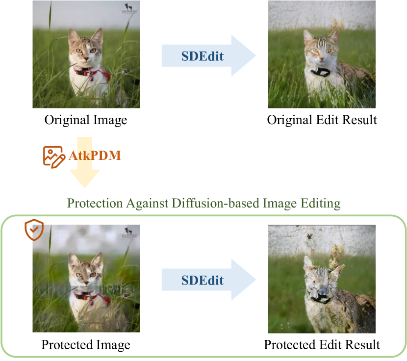
The malicious user collects an image from the internet and uses SDEdit (Meng et al. 2021) to generate unauthorized image translations or editing, denoted as , that manipulates the original input image .
Our work aims to safeguard the input image from the authorized manipulations by crafting an adversarial image by adding imperceptible perturbation to disrupt the reverse diffusion process of SDEdit for corrupted editions.
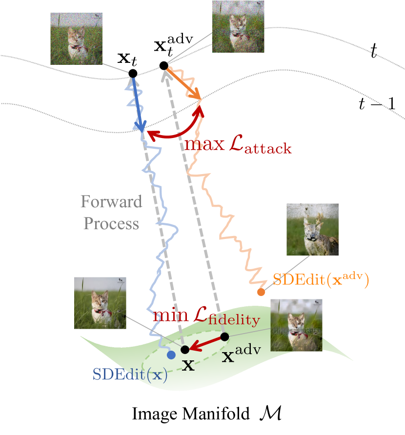
For example, we want the main object of the image, e.g., the cat in the source image as shown in Figure 2 unable to be reconstructed by the reverse diffusion process. Meanwhile, the adversarial image should maintain similarity to the source image to ensure fidelity. The reason why we target SDEdit as our threat model is that it is recognized as the most common and general operation in diffusion-based unconditional image translations and conditional image editing. Additionally, it has been incorporated into various editing pipelines (Tsaban and Passos 2023; Zhang et al. 2023). Here we focus on the unconditional image translations for our main study, as they are essential in both unconditional and conditional editing pipelines. Formally, our objective to effectively safeguard images while maintaining fidelity is formulated as:
| (2) | ||||
where indicates natural image manifold, , indicate image distance functions and denotes the fidelity budget.
In the following sections, we first present a conceptual illustration of our method, followed by our framework for solving the optimization problem. We then discuss the novel design of our attacking loss and fidelity constraints, which provide more efficient criteria compared to previous methods for solving the image protection optimization problem using PGD. Finally, we introduce an advanced design to enhance image protection quality by latent optimization via victim-model-agnostic VAE.
4.2 Overview
To achieve effective protection against diffusion-based editing, we aim to push the protected sample away from the original clean sample by disrupting the intermediate step in the reverse diffusion process. For practical real-world applications, it’s essential to ensure the protected image is perceptually similar to the original image. In practice, we uniformly sample the value of the forward diffusion step to generate noisy images and then perform optimization to craft the adversarial image via our attacking and fidelity losses, repeating the same process times or until convergence. Figure 2 depicts these two push-and-pull criteria during different noise levels, the successful attack is reflected in the light orange line where the reverse sample moves far away from the normal edition of the image. More specifically, our method can be formulated as follows:
| (3) | ||||
where denotes the attacking budget. The details of the attacking loss and the fidelity loss will be discussed in the following sections.
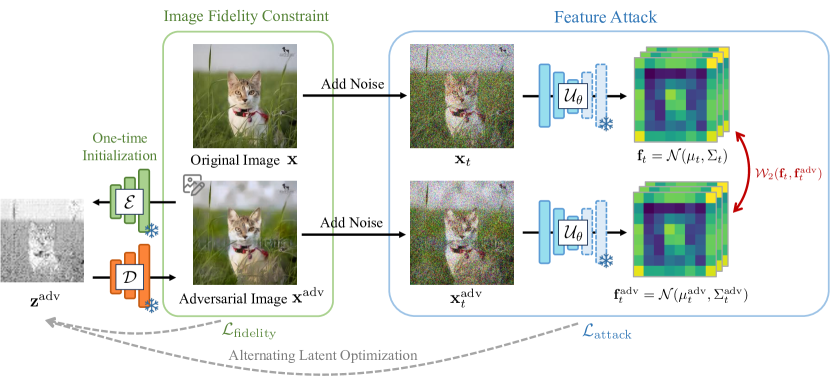
Framework.
Our framework is illustrated in Figure 3. We fix two identical victim UNets to extract feature representations of clean and protected samples for optimizing to push away from each other. A protection loss is jointly incorporated to constrain the optimization. After iterations, we segment out only the protecting main object of the image for better imperceptibility of image protection.
4.3 Proposed Losses
We propose two novel losses as optimization objectives to craft an adversarial example efficiently without running through all the diffusion steps. Attacking loss is designed to distract the feature representation in denoising UNet; Protection loss is a constraint to ensure the image quality. For notation simplicity, we first define the samples in different forwarded steps.
Let be the diffusion forward process. Given timestep sample from , noises sample from . We denote , and .
Attacking Loss.
Our goal is to define effective criteria that could finally distract the reverse denoising process. PhotoGuard (Salman et al. 2023) proposed to backpropagate through all the steps of the reverse denoising process via PGD, however, this approach is prohibitively expensive, Diff-Protect (Xue et al. 2024b) proposed to avoid the massive cost by leveraging Score Distillation (Poole et al. 2022) in optimization. However, Diff-protect relies heavily on gradients of attacking encoder of an LDM as stated in their results. In PDM, we don’t have such an encoder to attack; nevertheless, we find that the denoising UNet has a similar structure to encoder-decoder models, and some previous works (Lin and Yang 2024; Li et al. 2023) characterize this property to accelerate and enhance the generation. From our observations of the feature roles in denoising UNets, we hypothesize that distracting specific inherent feature representation in UNet blocks could lead to effectively crafting an adversarial image. In practice, we first extract the feature representations of forwarded images and in frozen UNet blocks of timestep . Then, we adopt 2-Wasserstein distance (Arjovsky, Chintala, and Bottou 2017) to measure the discrepancy in feature space. Note that we take the negative of the calculated distance, as we aim to pull the away from . Formally, the attacking loss is defined as:
| (4) |
Assuming the feature distributions approximate Gaussian distributions expressed by mean and , and non-singular covariance matrices and . The calculation of the 2-Wasserstein distance between two normal distributions is viable through the closed-form solution (Dowson and Landau 1982; Olkin and Pukelsheim 1982; Chen, Georgiou, and Tannenbaum 2018):
| (5) | ||||
Fidelity Loss.
To control the attack budget for adversarial image quality, we design a constraint function that utilizes the feature extractor from a pretrained classifier for calculating fidelity loss. In our case, we sum up the 2-Wasserstein feature losses of different layers. Specifically, we define as:
| (6) |
where denotes 2-Wasserstein distance and denotes layer of the feature extractor.
4.4 Alternating Optimization for Adversarial Image
We solve the constrained optimization problems via alternating optimization to craft the adversarial images, detailed optimization loop of AtkPDM+ is provided in Algorithm 1. AtkPDM algorithm and the derivation of the alternating optimization are provided in Appendix.
4.5 Latent Optimization via Pretrained-VAE
Previous works suggest that diffusion models have a strong capability of resisting adversarial perturbations (Xue and Chen 2024), making them hard to attack via pixel-domain optimization. Moreover, they are even considered good purifiers of adversarial perturbations (Nie et al. 2022). Here we propose a latent optimization strategy that crafts the “perturbation” in latent space. We adopt a pre-trained Variational Autoencoder (VAE) (Kingma and Welling 2014) to convert images to their latent space, and the gradients will be used to update the latent, after N iterations or losses converge, we decode back via decoder to pixel domain as our final protected image. The motivation for adopting VAE is inspired by MPGD (He et al. 2024). This strategy is effective for crafting a robust adversarial image against pixel-domain diffusion models while also better preserving the protection quality rather than only incorporating fidelity constraints. The constraint optimization thereby becomes:
| (7) | ||||
Detailed latent optimization loop is provided in Algorithm 1.
5 Experiment Results
In this section, we examine the attack effectiveness and robustness of our approach under extensive settings.
| Methods | Adversarial Image Quality | Attacking Effectiveness | ||||||
|---|---|---|---|---|---|---|---|---|
| SSIM | PSNR | LPIPS | SSIM | PSNR | LPIPS | IA-Score | ||
| Church | PGAscent | 0.37 0.09 | 28.17 0.22 | 0.73 0.16 | 0.89 0.05 | 31.06 1.94 | 0.17 0.09 | 0.93 0.04 |
| Diff-Protect | 0.39 0.07 | 28.03 0.12 | 0.67 0.11 | 0.82 0.05 | 31.90 1.08 | 0.23 0.07 | 0.91 0.04 | |
| AtkPDM (Ours) | 0.75 0.03 | 28.22 0.10 | 0.26 0.04 | 0.75 0.04 | 29.61 0.23 | 0.40 0.05 | 0.76 0.06 | |
| atkPDM+ (Ours) | 0.81 0.03 | 28.64 0.19 | 0.13 0.02 | 0.79 0.04 | 30.05 0.47 | 0.33 0.07 | 0.81 0.06 | |
| Cat | PGAscent | 0.48 0.09 | 28.34 0.18 | 0.65 0.12 | 0.96 0.02 | 32.32 2.49 | 0.10 0.05 | 0.97 0.03 |
| Diff-Protect | 0.33 0.10 | 28.03 0.15 | 0.80 0.15 | 0.90 0.05 | 33.94 1.93 | 0.18 0.08 | 0.95 0.03 | |
| atkPDM (Ours) | 0.71 0.06 | 28.47 0.18 | 0.29 0.05 | 0.83 0.03 | 30.73 0.51 | 0.39 0.05 | 0.81 0.04 | |
| atkPDM+ (Ours) | 0.83 0.04 | 29.41 0.37 | 0.09 0.02 | 0.93 0.01 | 33.02 0.74 | 0.18 0.02 | 0.92 0.01 | |
| Face | PGAscent | 0.48 0.05 | 28.75 0.18 | 0.64 0.10 | 0.99 0.00 | 37.96 1.75 | 0.02 0.01 | 0.99 0.00 |
| Diff-Protect | 0.25 0.04 | 28.09 0.20 | 0.91 0.11 | 0.95 0.02 | 35.33 1.62 | 0.08 0.04 | 0.96 0.02 | |
| atkPDM (Ours) | 0.56 0.04 | 28.01 0.22 | 0.36 0.04 | 0.74 0.03 | 29.14 0.36 | 0.40 0.05 | 0.62 0.07 | |
| atkPDM+ (Ours) | 0.81 0.04 | 28.39 0.20 | 0.12 0.03 | 0.86 0.03 | 30.26 0.72 | 0.24 0.07 | 0.80 0.08 | |
| Defense Method | Attacking Effectiveness | |||
|---|---|---|---|---|
| SSIM | PSNR | LPIPS | IA-Score | |
| Crop-and-Resize | 0.68 | 29.28 | 0.42 | 0.79 |
| JPEG Comp. | 0.78 | 29.82 | 0.36 | 0.79 |
| None | 0.79 | 30.05 | 0.33 | 0.81 |
5.1 Experiment Settings
Implementation Details.
We conduct all our experiments in white box settings and examine the effectiveness of our attacks using SDEdit (Meng et al. 2021). For the Variational Autoencoder (VAE) (Kingma and Welling 2014) in our AtkPDM+, we utilize the VAE provided by StableDiffusion V1.5 (Rombach et al. 2022). We run all of our experiments with 300 optimization steps, which is empirically determined, to balance attacking effectiveness and image protection quality with reasonable speed. Other loss parameters and running time are provided in the Appendix. The implementation is built on the Diffusers library. All the experiments are conducted with a single Nvidia Tesla V100 GPU.
Victim Models and Datasets.
We test our approach on PDMs with three open-source checkpoints on HuggingFace, specifically “google/ddpm-ema-church-256”, ”google/ddpm-cat-256” and “google/ddpm-ema-celebahq-256”. For the results reported in Table 1, we run 30 images for each victim model. Additionally, for generalizability in practical scenarios, we synthesize the data with half randomly from the originally trained dataset and another half from randomly crawled with keywords from the Internet.
Baseline Methods and Evaluation Metrics.
To the best of our knowledge, previous methods have mainly focused on LDMs, and effective PDM attacks have not yet been developed, however, we still implement Projected Gradient Ascent (PGAscent) with their proposed semantic loss by (Salman et al. 2023; Liang et al. 2023; Liang and Wu 2023; Xue et al. 2024b). Notably, Diff-Protect (Xue et al. 2024b) proposed to minimize the semantic loss is surprisingly better than maximizing the semantic loss, we also adopted this method in attacking PDMs and denote as Diff-Protect. To quantify the adversarial image visual quality, we adopted Structural Similarity (SSIM) (Wang et al. 2004), Peak Signal-to-Noise Ratio (PSNR), and Learned Perceptual Image Patch Similarity (LPIPS) (Zhang et al. 2018). We also inherit these three metrics, but negatively to quantify the effectiveness of our attack. We also adopted Image Alignment Score (IA-Score) (Kumari et al. 2023) that leverages CLIP (Radford et al. 2021) to calculate the cosine similarity of image encoder features. In distinguishing from previous methods, to more faithfully reflect the attack effectiveness, we fix the same seed of the random generator when generating clean and adversarial samples, then calculate the scores based on the paired samples.
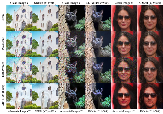
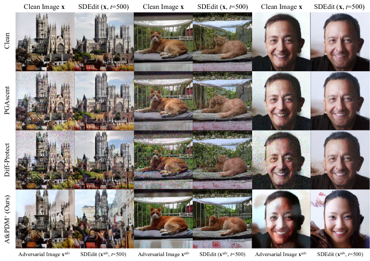
5.2 Attack Effectiveness on PDMs
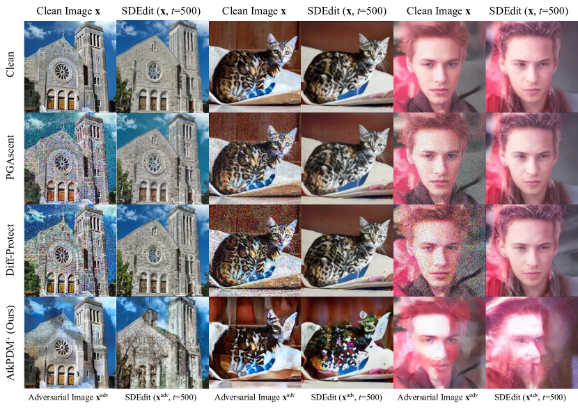
As quantitatively reported in Table 1 and qualitative results in Figure 4, compared to previous PGD-based methods incorporating semantic loss, i.e., negative training loss of diffusion models, our method exhibits superior performance in both adversarial image quality and attacking effectiveness. And our reported figures has generally stable as reflected in lower standard deviation. It is worth noting that even if the adversarial image qualities of the PGD-based methods are far worse than ours, their attacking effectiveness still falls short, suggesting that PDMs are robust against traditional perturbation methods, this finding is also aligned with previous works (Xue et al. 2024b; Xue and Chen 2024). For AtkPDM+, combined with our latent optimization strategy, the adversarial image quality has enhanced while slightly affecting the attacking effectiveness, still outperforming the previous methods.
| Setting | Attacking Effectiveness | |||
|---|---|---|---|---|
| SSIM | PSNR | LPIPS | IA-Score | |
| White Box | 0.79 | 30.05 | 0.33 | 0.81 |
| Black Box | 0.86 | 30.25 | 0.29 | 0.85 |
| Difference | 0.07 | 0.20 | 0.04 | 0.04 |
| Losses | VAE | Adversarial Image Quality | Attacking Effectiveness | |||||
| SSIM | PSNR | LPIPS | SSIM | PSNR | LPIPS | IA-Score | ||
| 0.37 0.09 | 28.17 0.22 | 0.73 0.16 | 0.89 0.05 | 31.06 1.94 | 0.17 0.09 | 0.93 0.04 | ||
| ✓ | 0.80 0.05 | 29.78 0.42 | 0.17 0.03 | 0.82 0.05 | 30.43 0.75 | 0.15 0.06 | 0.92 0.04 | |
| + | ✓ | 0.82 0.05 | 30.30 0.81 | 0.13 0.03 | 0.90 0.03 | 31.24 1.19 | 0.08 0.03 | 0.96 0.02 |
| + (Ours) | 0.75 0.03 | 28.22 0.10 | 0.26 0.04 | 0.75 0.04 | 29.61 0.23 | 0.40 0.05 | 0.76 0.06 | |
| + (Ours) | ✓ | 0.81 0.03 | 28.64 0.19 | 0.13 0.02 | 0.79 0.04 | 30.05 0.47 | 0.33 0.07 | 0.81 0.06 |
5.3 Against Defense Methods
We examine the robustness of our approach against two widely recognized and effective defense methods for defending against adversarial attacks as reported in Table 2.
Crop and Resize.
Noted by Diff-Protect, crop and resize is simple yet the most effective defense method against their attacks on LDMs. We also test our method against this defense using their settings, i.e., cropping 20% of the adversarial image and then resizing it to its original dimensions.
JPEG Compression.
Sandoval-Segura et al. (Sandoval-Segura, Geiping, and Goldstein 2023) demonstrated that JPEG compression is a simple yet effective adversarial defense method. In our experiments, we implement the JPEG compression at a quality setting of 25%. The quantitative results in Table 2 demonstrate that our method is robust against these two defense methods, with four of the metrics listed in Table 2 are not worse than no defenses. Surprisingly, these defense methods even make the adversarial image more effective than cases without defense.
5.4 Black Box Transferability
We craft adversarial images with the proxy model, “google/ddpm-ema-church-256”, in white-box settings and test their transferability to another “google/ddpm-bedroom-256” model for black-box attacks. Under identical validation settings, Table 3 reveals only a slight decrease in attack effectiveness metrics, indicating successful black-box transferability.
5.5 Effectiveness of Latent Optimization via VAE
We first incorporate our VAE latent optimization strategy in the previous semantic-loss-based PGAscent. From Table 4, without using , latent optimization has significantly enhanced the adversarial image quality and even slightly improved the attacking effectiveness. Adopting latent optimization in our approach enhances visual quality with a negligible decrease in attacking effectiveness. Surprisingly, incorporating our with current PGD-based method will drastically decrease the adversarial image quality despite its attack performing better than ours. This may be due to different constrained optimization problem settings.
6 Conclusion
In this paper, we present the first framework designed to effectively protect images manipulation by Pixel-domain Diffusion Models (PDMs). We demonstrate that while denoising UNets appear robust to conventional PGD-based attacks, their feature space remains vulnerable to attack. Our proposed feature attacking loss exploit the vulnerabilities to empower adversarial images to mislead PDMs, thereby producing low-quality output images. We approach this image protection problem as a constrained optimization problem, solving it through alternating optimization. Additionally, our latent optimization strategy via VAE enhances the naturalness of our adversarial images. Extensive experiments validate the efficacy of our method, achieving state-of-the-art performance in attacking PDMs.
References
- Arjovsky, Chintala, and Bottou (2017) Arjovsky, M.; Chintala, S.; and Bottou, L. 2017. Wasserstein generative adversarial networks. In International Conference on Machine Learning (ICML), 214–223.
- Chen, Georgiou, and Tannenbaum (2018) Chen, Y.; Georgiou, T. T.; and Tannenbaum, A. 2018. Optimal transport for Gaussian mixture models. IEEE Access, 7: 6269–6278.
- Dhariwal and Nichol (2021) Dhariwal, P.; and Nichol, A. 2021. Diffusion models beat gans on image synthesis. In Advances in Neural Information Processing Systems (NeurIPS), volume 34, 8780–8794.
- Dowson and Landau (1982) Dowson, D.; and Landau, B. 1982. The Fréchet distance between multivariate normal distributions. Journal of multivariate analysis, 12(3): 450–455.
- Goodfellow, Shlens, and Szegedy (2015) Goodfellow, I.; Shlens, J.; and Szegedy, C. 2015. Explaining and Harnessing Adversarial Examples. In International Conference on Learning Representations (ICLR).
- He et al. (2024) He, Y.; Murata, N.; Lai, C.-H.; Takida, Y.; Uesaka, T.; Kim, D.; Liao, W.-H.; Mitsufuji, Y.; Kolter, J. Z.; Salakhutdinov, R.; and Ermon, S. 2024. Manifold Preserving Guided Diffusion. In International Conference on Learning Representations (ICLR).
- Ho, Jain, and Abbeel (2020) Ho, J.; Jain, A.; and Abbeel, P. 2020. Denoising diffusion probabilistic models. In Advances in Neural Information Processing Systems (NeurIPS), volume 33, 6840–685.
- Kingma and Welling (2014) Kingma, D. P.; and Welling, M. 2014. Auto-Encoding Variational Bayes. In International Conference on Learning Representations (ICLR).
- Kumari et al. (2023) Kumari, N.; Zhang, B.; Zhang, R.; Shechtman, E.; and Zhu, J.-Y. 2023. Multi-concept customization of text-to-image diffusion. In Proceedings of the IEEE/CVF Conference on Computer Vision and Pattern Recognition (CVPR), 1931–1941.
- Laidlaw, Singla, and Feizi (2021) Laidlaw, C.; Singla, S.; and Feizi, S. 2021. Perceptual Adversarial Robustness: Defense Against Unseen Threat Models. In International Conference on Learning Representations (ICLR).
- Li et al. (2023) Li, S.; Hu, T.; Khan, F. S.; Li, L.; Yang, S.; Wang, Y.; Cheng, M.-M.; and Yang, J. 2023. Faster Diffusion: Rethinking the Role of UNet Encoder in Diffusion Models. arXiv preprint arXiv:2312.09608.
- Liang and Wu (2023) Liang, C.; and Wu, X. 2023. Mist: Towards Improved Adversarial Examples for Diffusion Models. arXiv preprint arXiv:2305.12683.
- Liang et al. (2023) Liang, C.; Wu, X.; Hua, Y.; Zhang, J.; Xue, Y.; Song, T.; Xue, Z.; Ma, R.; and Guan, H. 2023. Adversarial Example Does Good: Preventing Painting Imitation from Diffusion Models via Adversarial Examples. arXiv preprint arXiv:2302.04578.
- Lin and Yang (2024) Lin, S.; and Yang, X. 2024. Diffusion Model with Perceptual Loss. arXiv preprint arXiv:2401.00110.
- Liu et al. (2023) Liu, J.; Wei, C.; Guo, Y.; Yu, H.; Yuille, A.; Feizi, S.; Lau, C. P.; and Chellappa, R. 2023. Instruct2Attack: Language-Guided Semantic Adversarial Attacks. arXiv preprint arXiv:2311.15551.
- Lo et al. (2024) Lo, L.; Yeo, C. Y.; Shuai, H.-H.; and Cheng, W.-H. 2024. Distraction is All You Need: Memory-Efficient Image Immunization against Diffusion-Based Image Editing. In Proceedings of the IEEE/CVF Conference on Computer Vision and Pattern Recognition (CVPR), 24462–24471.
- Madry et al. (2018) Madry, A.; Makelov, A.; Schmidt, L.; Tsipras, D.; and Vladu, A. 2018. Towards deep learning models resistant to adversarial attacks. In International Conference on Learning Representations (ICLR).
- Meng et al. (2021) Meng, C.; He, Y.; Song, Y.; Song, J.; Wu, J.; Zhu, J.-Y.; and Ermon, S. 2021. Sdedit: Guided image synthesis and editing with stochastic differential equations. arXiv preprint arXiv:2108.01073.
- Nie et al. (2022) Nie, W.; Guo, B.; Huang, Y.; Xiao, C.; Vahdat, A.; and Anandkumar, A. 2022. Diffusion Models for Adversarial Purification. arXiv preprint arXiv:2312.09608.
- Olkin and Pukelsheim (1982) Olkin, I.; and Pukelsheim, F. 1982. The distance between two random vectors with given dispersion matrices. Linear Algebra and its Applications, 48: 257–263.
- Poole et al. (2022) Poole, B.; Jain, A.; Barron, J. T.; and Mildenhall, B. 2022. DreamFusion: Text-to-3D using 2D Diffusion. arXiv preprint arXiv:2209.14988.
- Radford et al. (2021) Radford, A.; Kim, J. W.; Hallacy, C.; Ramesh, A.; Goh, G.; Agarwal, S.; Sastry, G.; Askell, A.; Mishkin, P.; Clark, J.; et al. 2021. Learning transferable visual models from natural language supervision. In International Conference on Machine Learning (ICML), 8748–8763.
- Rombach et al. (2022) Rombach, R.; Blattmann, A.; Lorenz, D.; Esser, P.; and Ommer, B. 2022. High-resolution image synthesis with latent diffusion models. In Proceedings of the IEEE/CVF Conference on Computer Vision and Pattern Recognition (CVPR), 10684–10695.
- Ronneberger, Fischer, and Brox (2015) Ronneberger, O.; Fischer, P.; and Brox, T. 2015. U-net: Convolutional networks for biomedical image segmentation. In Medical Image Computing and Computer-Assisted Intervention (MICCAI), 234–241.
- Salman et al. (2023) Salman, H.; Khaddaj, A.; Leclerc, G.; Ilyas, A.; and Madry, A. 2023. Raising the Cost of Malicious AI-Powered Image Editing. arXiv preprint arXiv:2302.06588.
- Sandoval-Segura, Geiping, and Goldstein (2023) Sandoval-Segura, P.; Geiping, J.; and Goldstein, T. 2023. JPEG compressed images can bypass protections against ai editing. arXiv preprint arXiv:2304.02234.
- Shan et al. (2023) Shan, S.; Cryan, J.; Wenger, E.; Zheng, H.; Hanocka, R.; and Zhao, B. Y. 2023. Glaze: Protecting Artists from Style Mimicry by Text-to-Image Models. arXiv preprint arXiv:2302.04222.
- Shan et al. (2024) Shan, S.; Ding, W.; Passananti, J.; Wu, S.; Zheng, H.; and Zhao, B. Y. 2024. Nightshade: Prompt-Specific Poisoning Attacks on Text-to-Image Generative Models. arXiv preprint arXiv:2310.13828.
- Simonyan and Zisserman (2014) Simonyan, K.; and Zisserman, A. 2014. Very Deep Convolutional Networks for Large-Scale Image Recognition. CoRR.
- Song, Meng, and Ermon (2021) Song, J.; Meng, C.; and Ermon, S. 2021. Denoising diffusion implicit models. In International Conference on Learning Representations (ICLR).
- Song et al. (2020) Song, Y.; Garg, S.; Shi, J.; and Ermon, S. 2020. Sliced score matching: A scalable approach to density and score estimation. In Uncertainty in Artificial Intelligence, 574–584. PMLR.
- Tsaban and Passos (2023) Tsaban, L.; and Passos, A. 2023. LEDITS: Real Image Editing with DDPM Inversion and Semantic Guidance. arXiv:2307.00522.
- Wang et al. (2004) Wang, Z.; Bovik, A. C.; Sheikh, H. R.; and Simoncelli, E. P. 2004. Image quality assessment: from error visibility to structural similarity. IEEE Transactions on Image Processing, 13(4): 600–612.
- Wang, Zhao, and Xing (2023) Wang, Z.; Zhao, L.; and Xing, W. 2023. Stylediffusion: Controllable disentangled style transfer via diffusion models. In Proceedings of the IEEE/CVF International Conference on Computer Vision (ICCV), 7677–7689.
- Xue et al. (2024a) Xue, H.; Araujo, A.; Hu, B.; and Chen, Y. 2024a. Diffusion-based adversarial sample generation for improved stealthiness and controllability. In Advances in Neural Information Processing Systems (NeurIPS), volume 36.
- Xue and Chen (2024) Xue, H.; and Chen, Y. 2024. Pixel is a Barrier: Diffusion Models Are More Adversarially Robust Than We Think. arXiv preprint arXiv:2404.13320.
- Xue et al. (2024b) Xue, H.; Liang, C.; Wu, X.; and Chen, Y. 2024b. Toward effective protection against diffusion based mimicry through score distillation. arXiv preprint arXiv:2311.12832.
- Zhang et al. (2018) Zhang, R.; Isola, P.; Efros, A. A.; Shechtman, E.; and Wang, O. 2018. The unreasonable effectiveness of deep features as a perceptual metric. In Proceedings of the IEEE/CVF Conference on Computer Vision and Pattern Recognition (CVPR), 586–595.
- Zhang et al. (2023) Zhang, Y.; Huang, N.; Tang, F.; Huang, H.; Ma, C.; Dong, W.; and Xu, C. 2023. Inversion-based style transfer with diffusion models. In Proceedings of the IEEE/CVF Conference on Computer Vision and Pattern Recognition (CVPR), 10146–10156.
Supplementary Material
Appendix A More Implementation Details
The feature extractor for calculating is VGG16 (Simonyan and Zisserman 2014) with IMAGENET1K-V1 checkpoint. We use the SDEdit with the forward step for our main study results as it balances faithfulness to the original image and flexibility for editing. Empirically, we choose to randomly sample the forward step to enhance the optimization efficiency. The average time to optimize 300 steps for an image on a single Nvidia Tesla V100 is about 300 seconds. The estimated average memory usage is about 24GB. Table 5 provides the details of the step sizes that we use to attack different models.
| Models | Step Size | |
|---|---|---|
| () | () | |
| google/ddpm-ema-church-256 | ||
| google/ddpm-cat-256 | ||
| google/ddpm-ema-celebahq-256 | ||
Appendix B More Experimental Results
B.1 Attack Effectiveness on Latent Diffusion Models
We propose the feature representation attacking loss which can be adapted to target any UNet-based diffusion models. Hence, it is applicable to attack LDM using our proposed framework. We follow the evaluation settings of the previous works (Xue et al. 2024b) for fair comparisons. Quantitative results are shown in Table 6. Compared to previous LDM-specified methods, our method could achieve comparable results. This finding reflects the general vulnerability in UNet-based diffusion models that can be exploited to craft adversarial images against either PDMs or LDMs.
| Methods | Adversarial Image Quality | Attacking Effectiveness | ||||||
|---|---|---|---|---|---|---|---|---|
| SSIM | PSNR | LPIPS | SSIM | PSNR | LPIPS | IA-Score | ||
| Church | AdvDM () | 0.85 0.03 | 30.42 0.15 | 0.23 0.06 | 0.19 0.05 | 28.00 0.16 | 0.71 0.04 | 0.49 0.06 |
| Mist () | 0.81 0.03 | 29.45 0.13 | 0.25 0.05 | 0.14 0.03 | 27.95 0.13 | 0.76 0.04 | 0.48 0.05 | |
| Diff-Protect () | 0.79 0.03 | 29.92 0.15 | 0.24 0.06 | 0.15 0.03 | 28.00 0.14 | 0.71 0.04 | 0.48 0.05 | |
| Diff-Protect () | 0.79 0.04 | 29.47 0.11 | 0.26 0.06 | 0.17 0.04 | 28.00 0.15 | 0.69 0.04 | 0.49 0.06 | |
| AtkPDM (Ours) | 0.82 0.02 | 30.40 0.27 | 0.24 0.05 | 0.14 0.03 | 27.96 0.17 | 0.74 0.02 | 0.47 0.04 | |
| AtkPDM+ (Ours) | 0.61 0.07 | 29.17 0.32 | 0.20 0.02 | 0.27 0.06 | 28.07 0.18 | 0.66 0.05 | 0.51 0.06 | |
| Cat | AdvDM () | 0.86 0.04 | 30.68 0.24 | 0.25 0.09 | 0.21 0.05 | 28.03 0.21 | 0.70 0.07 | 0.53 0.04 |
| Mist () | 0.81 0.04 | 29.63 0.22 | 0.27 0.08 | 0.14 0.04 | 27.96 0.17 | 0.77 0.06 | 0.52 0.04 | |
| Diff-Protect () | 0.78 0.05 | 30.12 0.24 | 0.27 0.08 | 0.16 0.05 | 27.96 0.15 | 0.72 0.06 | 0.52 0.03 | |
| Diff-Protect () | 0.77 0.06 | 29.56 0.16 | 0.28 0.09 | 0.17 0.05 | 27.98 0.16 | 0.71 0.06 | 0.53 0.04 | |
| AtkPDM (Ours) | 0.84 0.02 | 30.79 0.49 | 0.25 0.07 | 0.18 0.04 | 28.00 0.19 | 0.72 0.05 | 0.52 0.03 | |
| AtkPDM+ (Ours) | 0.68 0.13 | 29.68 0.74 | 0.16 0.03 | 0.31 0.10 | 28.13 0.27 | 0.64 0.06 | 0.54 0.04 | |
| Face | AdvDM () | 0.83 0.02 | 30.81 0.22 | 0.32 0.06 | 0.26 0.05 | 28.07 0.28 | 0.74 0.05 | 0.47 0.07 |
| Mist () | 0.79 0.03 | 29.75 0.22 | 0.34 0.06 | 0.19 0.05 | 27.99 0.21 | 0.81 0.05 | 0.46 0.08 | |
| Diff-Protect () | 0.74 0.04 | 30.34 0.13 | 0.33 0.06 | 0.21 0.05 | 28.03 0.21 | 0.76 0.06 | 0.45 0.07 | |
| Diff-Protect () | 0.72 0.05 | 29.68 0.09 | 0.36 0.06 | 0.21 0.04 | 28.05 0.22 | 0.74 0.06 | 0.47 0.07 | |
| AtkPDM (Ours) | 0.83 0.02 | 31.21 0.44 | 0.31 0.05 | 0.21 0.04 | 28.03 0.26 | 0.78 0.04 | 0.44 0.06 | |
| AtkPDM+ (Ours) | 0.82 0.05 | 30.05 0.51 | 0.14 0.03 | 0.41 0.08 | 28.24 0.39 | 0.63 0.07 | 0.52 0.07 | |
B.2 Qualitative Demonstration of Corrupting UNet Feature during Sampling
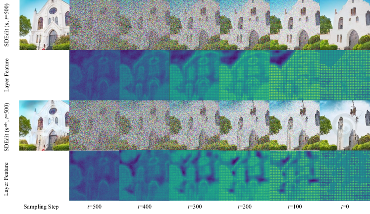
We qualitatively show an example of our attack effectiveness regarding UNet representation discrepancies in Figure 5. We compare a clean and an adversarial image using the same denoising process. Then, we take the feature maps of the second-last decoder block layer, close to the final predicted noise, to demonstrate their recognition of input image semantics. The results in Figure 5 show that from = 500, the feature maps of each pair start with a similar structure, then as the decreases, the feature maps gradually have higher discrepancies, suggesting our method, by attacking the middle representation of UNet, can effectively disrupt the reverse denoising process and mislead to corrupted samples.
B.3 Qualitative Results of Loss Ablation
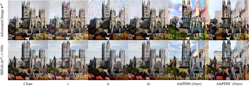
Figure 6 presents qualitative results of loss ablation where i., ii., and iii. indicate performing PGAscent with different configurations. i. utilizes only semantic loss; ii. utilizes semantic loss with our latent optimization strategy; iii. utilizes both semantic loss, our proposed and latent optimization. The results show that our and latent optimization can enhance the adversarial image quality of PGAscent. Moreover, comparing our proposed two methods, AtkPDM+ generates a more natural adversarial image than AtkPDM while maintaining attack effectiveness.
B.4 Different Forward Time-step Sampling
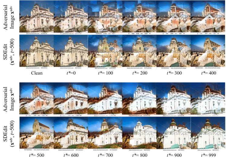
When using Monte Carlo sampling for optimization, the forward time step is sampled uniformly. We study the scenario that when is fixed for optimization. As shown in Figure 7, a primary result shows that when attacking to , the attacking effectiveness is better than other time steps. In practice, we can not know user-specified for editing in advance; however, this suggests that diffusion models have a potential temporal vulnerability that can be further exploited to increase efficiency.
B.5 More Qualitative Results
We provide more qualitative results in Figure 8 to showcase that our method can significantly change or corrupt the generated results with little modification on adversarial images. In contrast, previous methods add obvious perturbation to adversarial images but still fail to change the edited results to achieve the safeguarding goal.
B.6 Example of Loss Curves
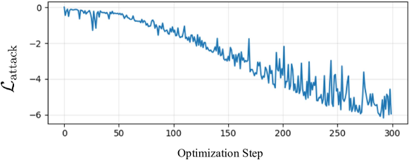
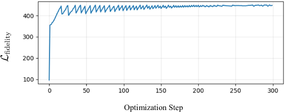
Figure 9 shows an example of our loss trends among optimization steps. has decreasing trend as the optimization step increases. has an increasing trend and converges to satisfy the constraint of the attack budget .
Appendix C Limitations
While our method can deliver acceptable attacks on PDMs, its visual quality is still not directly comparable to the results achieved on LDMs, indicating room for further improvement. More generalized PDM attacks should be further explored.
Appendix D Societal Impacts
Our work will not raise potential concerns about diffusion model abuses. Our work is dedicated to addressing these issues by safeguarding images from being infringed.
Appendix E Details of Our Proposed Algorithm
E.1 AtkPDM Algorithm without Latent Optimization
E.2 2-Wasserstein Distance Between Two Normal Distribution
Consider the normal distributions and . Let denote a joint distribution over the product space . The 2-Wasserstein distance between and is defined as:
Using properties of the mean and covariance, we have the following identities:
Thus, the 2-Wasserstein distance can be expressed as:
| (8) | ||||
where is the joint covariance matrix of and , defined as:
and is the covariance matrix between and :
By the Schur complement, the problem can be formulated as a semi-definite programming (SDP) problem:
| (9) | ||||
The closed-form solution for derived from the SDP is:
Finally, the closed-form solution for the 2-Wasserstein distance between the two normal distributions is given by:
| (10) | ||||
E.3 Alternating Optimization
Let , by Lagrange relaxation (Liu et al. 2023), the objective function can be expressed as:
| (11) |
where is the Lagrange multiplier and , are defined as
| (12) | ||||
| (13) |
The optimization is carried out in an alternating manner as follows:
| (14) | |||
| (15) |
To solve Equation 14, we employ the Fast Gradient Sign Method (FGSM) (Goodfellow, Shlens, and Szegedy 2015). The update is given by:
| (16) |
For Equation 15, we utilize Gradient Descent, resulting in the following update:
| (17) | |||
| (18) |
Note that the gradient of can be derived as follows:
where is indicator function with constraint .